A New Biased Estimator to Combat the Multicollinearity of the Gaussian Linear Regression Model

Abstract

In a multiple linear regression model, the ordinary least squares estimator is inefficient when the multicollinearity problem exists. Many authors have proposed different estimators to overcome the multicollinearity problem for linear regression models. This paper introduces a new regression estimator, called the Dawoud–Kibria estimator, as an alternative to the ordinary least squares estimator. Theory and simulation results show that this estimator performs better than other regression estimators under some conditions, according to the mean squares error criterion. The real-life datasets are used to illustrate the findings of the paper.

1. Introduction

Consider the following linear regression model:

$$y=X\beta +\epsilon ,$$

(1)

where $y$ is an $n\times 1$ vector of the dependent variable, $X$ is a known $n\times p$ full rank matrix of explanatory variables, and $\beta$ is a $p\times 1$ vector of unknown regression parameter. The ordinary least squares estimator (OLS) of $\beta$ in (1) is defined by

$$\widehat{\beta }=S^{-1}{X}^{\prime }y,$$

(2)

where $S=X^{\prime }X$ and $\epsilon$ is an $n\times 1$ vector of disturbances with zero mean and variance–covariance matrix, $Cov\left(\epsilon \right)={\sigma }^2{I}_n;$ $I_n$is an identity matrix of order nxn. Under the normality assumption of the disturbances, $\widehat{\beta }$ follows $N\left(\beta , {\sigma }^2{S}^{-1}\right)$ distribution.

In a multiple linear regression model, it is assumed that the explanatory variables are independent. However, in real-life situations, there may be strong or near-to-strong linear relationships among the explanatory variables. This causes the problem of multicollinearity. In the presence of multicollinearity, it is difficult to estimate the unique effect of individual variables in the regression equations. Moreover, the OLS estimator becomes unstable or inefficient and may produce the wrong sign (see Hoerl and Kennard) [1]. To overcome these problems, many authors have introduced different kinds of one- and two-parameter estimators: to mention a few, Stein [2], Massy [3], Hoerl and Kennard [1], Mayer and Willke [4], Swindel [5], Liu [6], Akdeniz and Kaçiranlar [7], Ozkale and Kaçiranlar [8], Sakallıoglu and Kaçıranlar [9], Yang and Chang [10], Roozbeh [11], Akdeniz and Roozbeh [12], Lukman et al. [13,14], and, very recently, Kibria and Lukman [15], among others.

The objective of this paper is to introduce a new class of two-parameter estimator for the regression parameter when the explanatory variables are correlated and then to compare the performance of the new estimator with the OLS estimator, the ordinary ridge regression (ORR) estimator, the Liu estimator, the Kibria–Lukman (KL) estimator, the two-parameter (TP) estimator proposed by Ozkale and Kaciranlar [8], and the new two-parameter (NTP) estimator that is proposed by Yang and Chang [10].

Some Alternative Biased Estimators and the Proposed Estimator

The canonical form of Equation (1) is as follows:

$$y=Z\alpha +\epsilon ,$$

(3)

where $Z=XP$ and $\alpha =P^{\prime }\beta$. Here, $P$ is an orthogonal matrix such that $Z^{\prime }Z=P^{\prime }{X}^{\prime }XP=\mathsf{\Lambda }=diag({\lambda }_1,{\lambda }_2,\dots ,{\lambda }_p).$ The OLS estimator of $\alpha$ is as follows:

$$\widehat{\alpha }={\mathsf{\Lambda }}^{-1}{Z}^{\prime }y,$$

(4)

and the mean squared error matrix (MSEM) of $\widehat{\alpha }$ is given by

$$MSEM(\widehat{\alpha })={\sigma }^2{\mathsf{\Lambda }}^{-1}.$$

(5)

The ORR of $\alpha$ [1] is given by

$$\widehat{\alpha }(k)=W(k)\widehat{\alpha },$$

(6)

where $W(k)={[I_p+k{\mathsf{\Lambda }}^{-1}]}^{-1}$, $k$ is the biasing parameter, and

$$MSEM(\widehat{\alpha }(k))={\sigma }^{2}W(k){\mathsf{\Lambda }}^{-1}W(k)+(W(k)-I_p)\alpha {\alpha }^{\prime }(W(k)-I_p{)}^{\prime }.$$

(7)

The Liu estimator of $\alpha$ [6] is given by

$$\widehat{\alpha }(d)=F(d)\widehat{\alpha },$$

(8)

where $F(d)={[\mathsf{\Lambda }+I_p]}^{-1}[\mathsf{\Lambda }+d{I}_p]$, $d$ is the biasing parameter of Liu estimator, and

$$MSEM(\widehat{\alpha }(d))={\sigma }^{2}F(d){\mathsf{\Lambda }}^{-1}{F}^{\prime }(d)+{(1-d)}^2{(\mathsf{\Lambda }+I_p)}^{-1}\alpha {\alpha }^{\prime }{(\mathsf{\Lambda }+I_p)}^{-1}.$$

(9)

The KL estimator of $\alpha$ [15] is given by

$${\widehat{\alpha }}_{KL}=W(k)M(k)\widehat{\alpha },$$

(10)

where $M(k)=[I_p-k{\mathsf{\Lambda }}^{-1}]$ and

$$\begin{array}{ll}MSEM({\widehat{\alpha }}_{KL})=& {\sigma }^{2}W(k)M(k){\mathsf{\Lambda }}^{-1}{M}^{\prime }(k)W^{\prime }(k)\\ & +[W(k)M(k)-I_p]\alpha {\alpha }^{\prime }[W(k)M(k)-I_p{]}^{\prime }\end{array}$$

(11)

The two-parameter (TP) estimator of $\alpha$ (Ozkale and Kaçiranlar [8]) is given by

$${\widehat{\alpha }}_{TP}=R\widehat{\alpha },$$

(12)

where $R={(\mathsf{\Lambda }+k{{\rm I}}_p)}^{-1}(\mathsf{\Lambda }+kd{{\rm I}}_p)$, $k$ and $d$ are the biasing parameters, and

$$MSEM({\widehat{\alpha }}_{TP})={\sigma }^{2}R{\mathsf{\Lambda }}^{-1}{R}^{\prime }+[R-I_p]\alpha {\alpha }^{\prime }[R-I_p{]}^{\prime }.$$

(13)

The new two-parameter (NTP) estimator of $\alpha$ (Yang, H.; Chang [10]) is given by

$${\widehat{\alpha }}_{NTP}=F(d)W(k)\widehat{\alpha },$$

(14)

$$MSEM({\widehat{\alpha }}_{NTP})={\sigma }^{2}F(d)W(k){\mathsf{\Lambda }}^{-1}{W}^{\prime }(k)F^{\prime }(d)+[F(d)W(k)-I_p]\alpha {\alpha }^{\prime }[F(d)W(k)-I_p{]}^{\prime }$$

(15)

The proposed new class of two-parameter estimator of $\alpha$ is obtained by minimizing $(y-Z\alpha {)}^{\prime }(y-Z\alpha )$, subject to $(\alpha +\widehat{\alpha }{)}^{\prime }(\alpha +\widehat{\alpha })=c$, where $c$ is a constant,

$$(y-Z\alpha {)}^{\prime }(y-Z\alpha )+k(1+d)[(\alpha +\widehat{\alpha }{)}^{\prime }(\alpha +\widehat{\alpha })-c].$$

(16)

Here, $k$ and $1+d$ are the Lagrangian multipliers.

The solution of minimizing the objective function

$$(y-Z\alpha {)}^{\prime }(y-Z\alpha )+k[(\alpha +\widehat{\alpha }{)}^{\prime }(\alpha +\widehat{\alpha })-c]$$

is obtained by Kibria and Lukman [15] for getting the KL estimator and defined in Equation (10).

Now, the solution to (16) gives the proposed estimator as follows:

$${\widehat{\alpha }}_{DK}={(Z^{\prime }Z+k(1+d){{\rm I}}_p)}^{-1}(Z^{\prime }Z-k(1+d){{\rm I}}_p)\widehat{\alpha }=W(k,d)M(k,d)\widehat{\alpha },$$

(17)

where $W(k,d)={[I_p+k(1+d){\mathsf{\Lambda }}^{-1}]}^{-1}$ and $M(k,d)=[I_p-k(1+d){\mathsf{\Lambda }}^{-1}]$.

The proposed estimator will be called the Dawoud–Kibria (DK) estimator and is denoted by ${\widehat{\alpha }}_{DK}$.

Moreover, the proposed DK estimator is also obtained by augmenting $-\sqrt{k}\sqrt{1+d}\widehat{\alpha }=\sqrt{k}\sqrt{1+d}\alpha +{\epsilon }^{\prime }$ to (3) and then using the OLS estimate. The MSEM of the DK estimator is given by

$$\begin{array}{ll}MSEM({\widehat{\alpha }}_{DK})=& {\sigma }^{2}W(k,d)M(k,d){\mathsf{\Lambda }}^{-1}{M}^{\prime }(k,d)W^{\prime }(k,d)\\ & +[W(k,d)M(k,d)-I_p]\alpha {\alpha }^{\prime }[W(k,d)M(k,d)-I_p{]}^{\prime }\end{array}$$

(18)

The main differences between the KL estimator and the proposed DK estimator are as follows:

-

The KL is a one-parameter estimator, while the proposed DK is a two-parameter estimator.

-

The KL estimator is obtained based on the objective function $(y-Z\alpha {)}^{\prime }(y-Z\alpha )+k[(\alpha +\widehat{\alpha }{)}^{\prime }(\alpha +\widehat{\alpha })-c]$, while the proposed DK estimator is obtained from a different objective function, which is $(y-Z\alpha {)}^{\prime }(y-Z\alpha )+k(1+d)[(\alpha +\widehat{\alpha }{)}^{\prime }(\alpha +\widehat{\alpha })-c]$.

-

The KL estimator is a function of the shrinkage estimator $k$, while the proposed DK estimator is a function of $k$ and $d$.

-

Since the KL estimator has one parameter and the proposed DK estimator has two parameters, their MSEs are different.

-

In the KL estimator, shrinkage parameter $k$ needs to be estimated, while in the proposed DK estimator, both $k$ and $d$ need to be estimated.

-

The KL estimator is a special case of the proposed DK estimator when $d=0$, so the proposed DK estimator is the general estimator.

The following lemmas will be used to make some theoretical comparisons among estimators in the following section.

Lemma 1 [16]. 

Let$n\times n$matrices$N>0$and $B>0$(or $B\ge 0$), then$N>B$if and only if${\lambda }_{\max }(B{N}^{-1})<1$, where${\lambda }_{\max }(B{N}^{-1})$is the maximum eigenvalue of matrix$B{N}^{-1.}$

Lemma 2 [17]. 

Let$B$be an$n\times n$positive definite matrix that is$B>0$and$\alpha$be some vector, then$B-\alpha {\alpha }^{\prime }>0$if and only if${\alpha }^{\prime }{B}^{-1}\alpha <1$.

Lemma 3 [18]. 

Let${\alpha }_i=B_{i}y$,$i=1,2$be two linear estimators of$\alpha$. Suppose that$D=Cov({\widehat{\alpha }}_1)-Cov({\widehat{\alpha }}_2)>0$, where$Cov({\widehat{\alpha }}_i)i=1,2$is the covariance matrix of${\widehat{\alpha }}_i$and$b_i=Bias({\widehat{\alpha }}_i)=(B_{i}X-I)\alpha$, $i=1,2$. Consequently,

$$\Delta ({\widehat{\alpha }}_1-{\widehat{\alpha }}_2)=MSEM({\widehat{\alpha }}_1)-MSEM({\widehat{\alpha }}_2)={\sigma }^{2}D+b_1{b^{\prime }}_1-b_2{b^{\prime }}_2>0$$

(19)

if and only if${b^{\prime }}_2[{\sigma }^{2}D+{b^{\prime }}_1{b}_1]b_2<1$, where$MSEM({\widehat{\alpha }}_i)=Cov({\widehat{\alpha }}_i)+b_i{b^{\prime }}_i$.

The rest of this article is organized as follows: In Section 2, we give the theoretical comparisons among the abovementioned estimators and derive the biasing parameters of the proposed DK estimator. A simulation study is conducted in Section 3. Two numerical examples are illustrated in Section 4. Finally, some concluding remarks are given in Section 5.

2. Comparison among the Estimators

2.1. Theoretical Comparisons among the Proposed DK Estimator and the OLS, ORR, Liu, KL, TP, and NTP Estimators

Theorem 1.

The proposed estimator ${\widehat{\alpha }}_{DK}$is superior to estimator $\widehat{\alpha }$if and only if

$$\begin{array}{c}{\alpha }^{\prime }[W(k,d)M(k,d)-I_p{]}^{\prime }[{\sigma }^2({\mathsf{\Lambda }}^{-1}-W(k,d)M(k,d){\mathsf{\Lambda }}^{-1}{M}^{\prime }(k,d)W^{\prime }(k,d))]\\ [W(k,d)M(k,d)-I_p]\alpha <1.\end{array}$$

(20)

Proof. 

The difference of the dispersion matrices is given by

$$\begin{array}{c}D(\widehat{\alpha })-D({\widehat{\alpha }}_{DK})={\sigma }^2({\mathsf{\Lambda }}^{-1}-W(k,d)M(k,d){\mathsf{\Lambda }}^{-1}{M}^{\prime }(k,d)W^{\prime }(k,d))\\ ={\sigma }^{2}diag{\{\frac{1}{{\lambda }_i}-\frac{{({\lambda }_i-k(1+d))}^2}{{\lambda }_i{({\lambda }_i+k(1+d))}^2}\}}_{i=1}^p\end{array}$$

(21)

where

$${\mathsf{\Lambda }}^{-1}-W(k,d)M(k,d){\mathsf{\Lambda }}^{-1}{M}^{\prime }(k,d)W^{\prime }(k,d)$$

will be positive definite (pd) if and only if

$${({\lambda }_i+k(1+d))}^2-{({\lambda }_i-k(1+d))}^2>0.$$

We observed that for $k>0$ and $0<d<1$,

$${({\lambda }_i+k(1+d))}^2-{({\lambda }_i-k(1+d))}^2=4k(1+d){\lambda }_i>0.$$

Consequently, ${\mathsf{\Lambda }}^{-1}-W(k,d)M(k,d){\mathsf{\Lambda }}^{-1}{M}^{\prime }(k,d)W^{\prime }(k,d)$ is positive definite. □

Theorem 2.

When${\lambda }_{\max }(H{G}^{-1})<1$, the proposed estimator ${\widehat{\alpha }}_{DK}$is superior to estimator $\widehat{\alpha }(k)$if and only if

$$\begin{array}{c}{\alpha }^{\prime }[W(k,d)M(k,d)-I_p{]}^{\prime }[V_1+(W(k)-I_p)\alpha {\alpha }^{\prime }(W(k)-I_p{)}^{\prime }]\\ [W(k,d)M(k,d)-I_p]\alpha <1\end{array}$$

(22)

$${\lambda }_{\max }(H{G}^{-1})<1,$$

(23)

where

$$V_1={\sigma }^2(W(k){\mathsf{\Lambda }}^{-1}{W}^{\prime }(k)-W(k,d)M(k,d){\mathsf{\Lambda }}^{-1}{M}^{\prime }(k,d)W^{\prime }(k,d)),$$

$$H=W(k,d)\mathsf{\Lambda }{W}^{\prime }(k,d)+k^2{(1+d)}^{2}W(k,d){\mathsf{\Lambda }}^{-1}{W}^{\prime }(k,d),$$

$$G=W(k)\mathsf{\Lambda }{W}^{\prime }(k)+2k(1+d)W(k,d)W^{\prime }(k,d).$$

Proof. 

$$\begin{array}{l}{V}_1={\sigma }^2(W(k){\mathsf{\Lambda }}^{-1}{W}^{\prime }(k)-W(k,d)M(k,d){\mathsf{\Lambda }}^{-1}{M}^{\prime }(k,d)W^{\prime }(k,d))\\ ={\sigma }^2(W(k){\mathsf{\Lambda }}^{-1}{W}^{\prime }(k)-W(k,d)(I_p-k(1+d){\mathsf{\Lambda }}^{-1}){\mathsf{\Lambda }}^{-1}(I_p-k(1+d){\mathsf{\Lambda }}^{-1})W^{\prime }(k,d))\\ ={\sigma }^2{\mathsf{\Lambda }}^{-1}(W(k)\mathsf{\Lambda }{W}^{\prime }(k)+2k(1+d)W(k,d)W^{\prime }(k,d)\\ -(W(k,d)\mathsf{\Lambda }{W}^{\prime }(k,d)+k^2{(1+d)}^{2}W(k,d){\mathsf{\Lambda }}^{-1}{W}^{\prime }(k,d))){\mathsf{\Lambda }}^{-1}\\ ={\sigma }^2{\mathsf{\Lambda }}^{-1}(G-H){\mathsf{\Lambda }}^{-1}.\end{array}$$

It is clear that for $k>0$ and $0<d<1$, $G>0$ and $H>0$. It is obvious that $G-H>0$ if and only if

$${\lambda }_{\max }(H{G}^{-1})<1,$$

where ${\lambda }_{\max }(H{G}^{-1})$ is the maximum eigenvalue of the matrix $H{G}^{-1}$. Consequently, $V_1$ is positive definite. □

Theorem 3.

The proposed estimator ${\widehat{\alpha }}_{DK}$is superior to estimator $\widehat{\alpha }(d)$if and only if

$$\begin{array}{c}{\alpha }^{\prime }[W(k,d)M(k,d)-I_p{]}^{\prime }[V_2+{(1-d)}^2{(\mathsf{\Lambda }+I_p)}^{-1}\alpha {\alpha }^{\prime }{(\mathsf{\Lambda }+I_p)}^{-1}]\\ [W(k,d)M(k,d)-I_p]\alpha <1\end{array}$$

(24)

where $V_2={\sigma }^2(F(d){\mathsf{\Lambda }}^{-1}{F}^{\prime }(d)-W(k,d)M(k,d){\mathsf{\Lambda }}^{-1}{M}^{\prime }(k,d)W^{\prime }(k,d))$.

Proof. 

Using the difference between the dispersion matrices

$$\begin{array}{l}{V}_2={\sigma }^2(F(d){\mathsf{\Lambda }}^{-1}{F}^{\prime }(d)-W(k,d)M(k,d){\mathsf{\Lambda }}^{-1}{M}^{\prime }(k,d)W^{\prime }(k,d))\\ ={\sigma }^{2}diag{\{\frac{{({\lambda }_i+d)}^2}{{\lambda }_i{({\lambda }_i+1)}^2}-\frac{{({\lambda }_i-k(1+d))}^2}{{\lambda }_i{({\lambda }_i+k(1+d))}^2}\}}_{i=1}^p\end{array}$$

(25)

where

$$F(d){\mathsf{\Lambda }}^{-1}{F}^{\prime }(d)-W(k,d)M(k,d){\mathsf{\Lambda }}^{-1}{M}^{\prime }(k,d)W^{\prime }(k,d)$$

will be pd if and only if

$$\begin{gathered} {({\lambda }_i+k(1+d))}^2{({\lambda }_i+d)}^2-{({\lambda }_i-k(1+d))}^2{({\lambda }_i+1)}^2>0\mathrm{or} \\ ({\lambda }_i+k(1+d))({\lambda }_i+d)-({\lambda }_i-k(1+d))({\lambda }_i+1)>0. \end{gathered}$$

So, if $k>0$ and $0<d<1$, $({\lambda }_i+k(1+d))({\lambda }_i+d)-({\lambda }_i-k(1+d))({\lambda }_i+1)=k(1+d)(2{\lambda }_i+d+1)+{\lambda }_i(d-1)>0$. Consequently,

$$F(d){\mathsf{\Lambda }}^{-1}{F}^{\prime }(d)-W(k,d)M(k,d){\mathsf{\Lambda }}^{-1}{M}^{\prime }(k,d)W^{\prime }(k,d)$$

is positive definite. □

Theorem 4.

The proposed estimator ${\widehat{\alpha }}_{DK}$is superior to estimator${\widehat{\alpha }}_{KL}$if and only if

$$\begin{array}{c}{\alpha }^{\prime }[W(k,d)M(k,d)-I_p{]}^{\prime }[V_3+[W(k)M(k)-I_p]\alpha {\alpha }^{\prime }[W(k)M(k)-I_p{]}^{\prime }]\\ [W(k,d)M(k,d)-I_p]\alpha <1\end{array}$$

(26)

where $V_3={\sigma }^2(W(k)M(k){\mathsf{\Lambda }}^{-1}{M}^{\prime }(k)W^{\prime }(k)-W(k,d)M(k,d){\mathsf{\Lambda }}^{-1}{M}^{\prime }(k,d)W^{\prime }(k,d))$.

Proof. 

Using the difference between the dispersion matrices

$$\begin{array}{l}{V}_3={\sigma }^2(W(k)M(k){\mathsf{\Lambda }}^{-1}{M}^{\prime }(k)W^{\prime }(k)-W(k,d)M(k,d){\mathsf{\Lambda }}^{-1}{M}^{\prime }(k,d)W^{\prime }(k,d))\\ ={\sigma }^{2}diag{\{\frac{{({\lambda }_i-k)}^2}{{\lambda }_i{({\lambda }_i+k)}^2}-\frac{{({\lambda }_i-k(1+d))}^2}{{\lambda }_i{({\lambda }_i+k(1+d))}^2}\}}_{i=1}^p,\end{array}$$

(27)

where

$$W(k)M(k){\mathsf{\Lambda }}^{-1}{M}^{\prime }(k)W^{\prime }(k)-W(k,d)M(k,d){\mathsf{\Lambda }}^{-1}{M}^{\prime }(k,d)W^{\prime }(k,d)$$

will be pd if and only if

$$\begin{gathered} {({\lambda }_i+k(1+d))}^2{({\lambda }_i-k)}^2-{({\lambda }_i-k(1+d))}^2{({\lambda }_i+k)}^2>0\mathrm{or} \\ ({\lambda }_i+k(1+d))({\lambda }_i-k)-({\lambda }_i-k(1+d))({\lambda }_i+k)>0. \end{gathered}$$

Obviously, for $k>0$ and $0<d<1$,

$$({\lambda }_i+k(1+d))({\lambda }_i-k)-({\lambda }_i-k(1+d))({\lambda }_i+k)=2kd{\lambda }_i>0.$$

Consequently,

$$W(k)M(k){\mathsf{\Lambda }}^{-1}{M}^{\prime }(k)W^{\prime }(k)-W(k,d)M(k,d){\mathsf{\Lambda }}^{-1}{M}^{\prime }(k,d)W^{\prime }(k,d)$$

is positive definite. □

Theorem 5.

The proposed estimator ${\widehat{\alpha }}_{DK}$is superior to estimator ${\widehat{\alpha }}_{TP}$if and only if

$${\alpha }^{\prime }[W(k,d)M(k,d)-I_p{]}^{\prime }[V_4+(R-I_p)\alpha {\alpha }^{\prime }(R-I_p{)}^{\prime }][W(k,d)M(k,d)-I_p]\alpha <1$$

(28)

where $V_4={\sigma }^2(R{\mathsf{\Lambda }}^{-1}{R}^{\prime }-W(k,d)M(k,d){\mathsf{\Lambda }}^{-1}{M}^{\prime }(k,d)W^{\prime }(k,d))$.

Proof.  

$$\begin{array}{l}{V}_4={\sigma }^2(R{\mathsf{\Lambda }}^{-1}{R}^{\prime }-W(k,d)M(k,d){\mathsf{\Lambda }}^{-1}{M}^{\prime }(k,d)W^{\prime }(k,d))\\ ={\sigma }^{2}diag{\{\frac{{({\lambda }_i+kd)}^2}{{\lambda }_i{({\lambda }_i+k)}^2}-\frac{{({\lambda }_i-k(1+d))}^2}{{\lambda }_i{({\lambda }_i+k(1+d))}^2}\}}_{i=1}^p,\end{array}$$

(29)

where

$$R{\mathsf{\Lambda }}^{-1}{R}^{\prime }-W(k,d)M(k,d){\mathsf{\Lambda }}^{-1}{M}^{\prime }(k,d)W^{\prime }(k,d)$$

will be positive definite if and only if

$$\begin{gathered} {({\lambda }_i+kd)}^2{({\lambda }_i+k(1+d))}^2-{({\lambda }_i+k)}^2{({\lambda }_i-k(1+d))}^2>0\mathrm{or} \\ ({\lambda }_i+kd)({\lambda }_i+k(1+d))-({\lambda }_i+k)({\lambda }_i-k(1+d))>0. \end{gathered}$$

Clearly, for $k>0$ and $0<d<1$, $({\lambda }_i+kd)({\lambda }_i+k(1+d))-({\lambda }_i+k)({\lambda }_i-k(1+d))={\lambda }_{i}k(3d+1)+k^2{(1+d)}^2>0$. Consequently, $R{\mathsf{\Lambda }}^{-1}{R}^{\prime }-W(k,d)M(k,d){\mathsf{\Lambda }}^{-1}{M}^{\prime }(k,d)W^{\prime }(k,d)$ is pd. □

Theorem 6.

The proposed estimator ${\widehat{\alpha }}_{DK}$is superior to estimator${\widehat{\alpha }}_{NTP}$if and only if

$$\begin{array}{c}{\alpha }^{\prime }[W(k,d)M(k,d)-I_p{]}^{\prime }[V_5+(F(d)W(k)-I_p)\alpha {\alpha }^{\prime }(F(d)W(k)-I_p{)}^{\prime }]\\ [W(k,d)M(k,d)-I_p]\alpha <1\end{array}$$

(30)

where $V_5={\sigma }^2(F(d)W(k){\mathsf{\Lambda }}^{-1}{W}^{\prime }(k)F^{\prime }(d)-W(k,d)M(k,d){\mathsf{\Lambda }}^{-1}{M}^{\prime }(k,d)W^{\prime }(k,d))$.

Proof. 

$$\begin{array}{l}{V}_5={\sigma }^2(F(d)W(k){\mathsf{\Lambda }}^{-1}{W}^{\prime }(k)F^{\prime }(d)-W(k,d)M(k,d){\mathsf{\Lambda }}^{-1}{M}^{\prime }(k,d)W^{\prime }(k,d))\\ ={\sigma }^{2}diag{\{\frac{{\lambda }_i{({\lambda }_i+d)}^2}{{({\lambda }_i+1)}^2{({\lambda }_i+k)}^2}-\frac{{({\lambda }_i-k(1+d))}^2}{{\lambda }_i{({\lambda }_i+k(1+d))}^2}\}}_{i=1}^p,\end{array}$$

(31)

where

$$F(d)W(k){\mathsf{\Lambda }}^{-1}{W}^{\prime }(k)F^{\prime }(d)-W(k,d)M(k,d){\mathsf{\Lambda }}^{-1}{M}^{\prime }(k,d)W^{\prime }(k,d)$$

will be pd if and only if

$$\begin{gathered} {\lambda }_i^2{({\lambda }_i+d)}^2{({\lambda }_i+k(1+d))}^2-{({\lambda }_i+1)}^2{({\lambda }_i+k)}^2{({\lambda }_i-k(1+d))}^2>0\mathrm{or} \\ {\lambda }_i({\lambda }_i+d)({\lambda }_i+k(1+d))-({\lambda }_i+1)({\lambda }_i+k)({\lambda }_i-k(1+d))>0. \end{gathered}$$

Clearly, for $k>0$ and $0<d<1$,

$$\begin{gathered} {\lambda }_i({\lambda }_i+d)({\lambda }_i+k(1+d))-({\lambda }_i+1)({\lambda }_i+k)({\lambda }_i-k(1+d))) \\ ={\lambda }_i^2(k(1+2d)+d-1)+{\lambda }_i(kd(2+d+k)+k^2)+k^2(1+d). \end{gathered}$$

Consequently, $F(d)W(k){\mathsf{\Lambda }}^{-1}{W}^{\prime }(k)F^{\prime }(d)-W(k,d)M(k,d){\mathsf{\Lambda }}^{-1}{M}^{\prime }(k,d)W^{\prime }(k,d)$ is positive definite. □

2.2. Determination of the Parameters k and d

Since both biasing parameters $k$ and $d$ are unknown and need to be estimated from the observed data, we will give a short discussion on the estimation of the parameters in this subsection. The biasing parameter $k$ in the ORR estimator and the biasing parameter $d$ in the Liu estimator were derived by Hoerl and Kennard [1] and Liu [6], respectively. Different authors for different kinds of models have proposed different estimators of $k$ and $d$: to mention a few, Hoerl et al. [19], Kibria [20], Kibria and Banik [21], Lukman and Ayinde [22], Mansson et al. [23], and Khalaf and Shukur [24], among others.

Now, we will discuss the estimation of the optimal values of $k$ and $d$ for the proposed DK estimator. First, we assume that $d$ is fixed, then the optimal value of $k$ can be obtained by minimizing

$$MSEM({\widehat{\alpha }}_{DK})=E(({\widehat{\alpha }}_{DK}-\alpha {)}^{\prime }({\widehat{\alpha }}_{DK}-\alpha )),$$

$$m(k,d)=tr(MSEM({\widehat{\alpha }}_{DK})),$$

$$m(k,d)={\sigma }^2{\displaystyle \sum _{i=1}^p\frac{{({\lambda }_i-k(1+d))}^2}{{\lambda }_i{({\lambda }_i+k(1+d))}^2}}+4k^2{(1+d)}^2{\displaystyle \sum _{i=1}^p\frac{{\alpha }_i^2}{{({\lambda }_i+k(1+d))}^2}}$$

(32)

Differentiating $m(k,d)$ with respect to $k$ and setting $(\partial m(k,d)/\partial k)=0$, we obtain

$$k=\frac{{\sigma }^2}{(1+d)(\raisebox{1ex}{${\sigma }^2$}\!\left/ \!\raisebox{-1ex}{${\lambda }_i$}\right.+2{\alpha }_i^2)}$$

(33)

Since the optimal value of $k$ in (33) depends on the unknown parameters ${\sigma }^2$ and ${\alpha }_i^2$, we replace them with their corresponding unbiased estimators. Consequently, we have

$$\widehat{k}=\frac{{\widehat{\sigma }}^2}{(1+d)(\raisebox{1ex}{${\widehat{\sigma }}^2$}\!\left/ \!\raisebox{-1ex}{${\lambda }_i$}\right.+2{\widehat{\alpha }}_i^2)}$$

(34)

and

$${\widehat{k}}_{\min }(DK)=\min {\left\{\frac{{\widehat{\sigma }}^2}{(1+d)({\widehat{\sigma }}^2/{\lambda }_i+(2{\widehat{\alpha }}_i^2))}\right\}}_{i=1}^p$$

(35)

Furthermore, the optimal value of $d$ can be obtained by differentiating $m(k,d)$ with respect to $d$ for a fixed $k$ and setting $(\partial m(k,d)/\partial d)=0$, and we obtain

$$d=\frac{{\sigma }^2{\lambda }_i}{m}-1,$$

(36)

where $m=k({\sigma }^2+2{\lambda }_i{\alpha }_i^2)$.

Additionally, the optimal $d$ with known parameters is

$$\widehat{d}=\frac{{\widehat{\sigma }}^2{\lambda }_i}{\widehat{m}}-1,$$

(37)

where $\widehat{m}=\widehat{k}({\widehat{\sigma }}^2+2{\lambda }_i{\widehat{\alpha }}_i^2)$.

In addition,

$${\widehat{d}}_{\min }(DK)={\left\{\frac{{\widehat{\sigma }}^2{\lambda }_i}{{\widehat{k}}_{\min }(DK)({\widehat{\sigma }}^2+2{\lambda }_i{\widehat{\alpha }}_i^2)}-1\right\}}_{i=1}^p$$

(38)

The estimator determination of the parameters $k$ and $d$ in ${\widehat{\alpha }}_{DK}$ is obtained iteratively as follows:

Step 1: Obtain an initial estimate of $d$ using $\widehat{d}=\min (\frac{{\widehat{\sigma }}^2}{{\widehat{\alpha }}_i^2})$.

Step 2: Obtain ${\widehat{k}}_{\min }(DK)$ from (35) using $\widehat{d}$ in Step 1.

Step 3: Estimate ${\widehat{d}}_{\min }(DK)$ in (38) by using ${\widehat{k}}_{\min }(DK)$ in Step 2.

Step 4: In case ${\widehat{d}}_{\min }(DK)$ is not between 0 and 1, use ${\widehat{d}}_{\min }(DK)=\widehat{d}$.

Additionally, Hoerl et al. [19] defined the biasing parameter k for the ORR estimator as

$$\widehat{k}=\frac{p{\widehat{\sigma }}^2}{{\displaystyle \sum _{i=1}^p{\widehat{\alpha }}_i^2}}$$

(39)

The biasing parameter d is given by Ozkale and Kaciranlar [8] and adopted for the Liu estimator

$$\widehat{d}=\min \left(\frac{{\widehat{\sigma }}^2}{{\widehat{\alpha }}_i^2+\frac{{\widehat{\sigma }}^2}{{\lambda }_i}}\right)$$

(40)

Then, Kibria and Lukman [15] found the biasing parameter estimator for the KL estimator as

$${\widehat{k}}_{\min }=\min \left(\frac{{\widehat{\sigma }}^2}{2{\widehat{\alpha }}_i^2+\frac{{\widehat{\sigma }}^2}{{\lambda }_i}}\right)$$

(41)

In addition, ${\widehat{k}}_{\min }$ of the KL estimator is also obtained when $d=0$ in the derived biasing parameter estimator ${\widehat{k}}_{\min }(DK)$ for the proposed DK estimator.

3. Simulation Study

To support a theoretical comparison of the estimators, a Monte Carlo simulation study was conducted to compare the performance of the estimators in this section. As such, this section will contain (i) the simulation technique and (ii) a discussion of the results.

3.1. Simulation Technique

Following Gibbons [25] and Kibria [20], we generated the explanatory variables using the following equation:

$$x_{ij}={(1-{\rho }^2)}^{1/2}{z}_{ij}+\rho z_{i,p+1},i=1,2,\dots ,n,j=1,2,\dots ,p$$

(42)

where $z_{ij}$ are independent standard normal pseudo-random numbers, and $\rho$ represents the correlation between any two explanatory variables and is considered here to be 0.90 and 0.99. We consider $p=3$ in the simulation. These variables are standardized so that $X^{\prime }X$ and $X^{\prime }y$ are in correlation forms. The $n$ observations for the dependent variable $y$ are determined by the following equation:

$$y_i={\beta }_1{x}_{i1}+{\beta }_2{x}_{i2}+\dots +{\beta }_p{x}_{ip}+e_i,i=1,2,\dots ,n$$

(43)

where $e_i$ are $i.i.dN(0,{\sigma }^2)$. The values of $\beta$ are chosen such that ${\beta }^{\prime }\beta =1$ [26]. Since we aimed to compare the performance of the DK estimator with OLS, ORR, Liu, KL, TP, and NTP estimators, we chose $k$ (0.3, 0.6, 0.9) between 0 and 1, as did Wichern and Churchill [27] and Kan et al. [28], where ORR gives better results and $d$ (0.2, 0.5, 0.8). The replication of this simulation study is 1000 times for the sample sizes $n=50$ and 100 and ${\sigma }^2=$ 1, 25, and 100. For each replicate, we computed the mean square error (MSE) of the estimators by using the equation below:

$$MSE({\alpha }^{*})=\frac{1}{1000}{\displaystyle \sum _{j=1}^{1000}({\alpha }_{ij}^{*}-{\alpha }_i{)}^{\prime }({\alpha }_{ij}^{*}-{\alpha }_i)}$$

(44)

where ${\alpha }_{ij}^{*}$ is the estimator values and ${\alpha }_i$ is the true parameter values. The estimated MSEs of the estimators are shown in Table 1, Table 2, Table 3 and Table 4.

Table 1. Estimated MSE for ordinary least squares estimator (OLS), ordinary ridge regression (ORR), Liu, Kibria–Lukman (KL), two-parameter (TP), new two-parameter (NTP), and Dawoud–Kibria (DK).

$\mathit{\rho }=0.90,\mathit{n}=50$
$\mathit{k}$	$\mathit{d}$	$\mathit{\sigma }$	OLS	ORR	Liu	KL	TP	NTP	DK
0.3	0.2	1	0.2136	0.2005	0.1821	0.1879	0.2031	0.1711	0.1832
		5	5.3394	5.0135	4.5507	4.6982	5.0778	4.2749	4.5799
		10	21.357	20.054	18.203	18.793	20.311	17.099	18.319
	0.5	1	0.2136	0.2005	0.1936	0.1879	0.2070	0.1818	0.1764
		5	5.3394	5.0135	4.8388	4.6982	5.1751	4.5446	4.4080
		10	21.357	20.054	19.355	18.793	20.700	18.178	17.632
	0.8	1	0.2136	0.2005	0.2054	0.1879	0.2109	0.1929	0.1698
		5	5.3394	5.0135	5.1361	4.6982	5.2734	4.8231	4.2427
		10	21.357	20.054	20.544	18.793	21.093	19.292	16.970
0.6	0.2	1	0.2136	0.1887	0.1821	0.1655	0.1936	0.1611	0.1574
		5	5.3394	4.7176	4.5507	4.1361	4.8388	4.0245	3.9308
		10	21.357	18.870	18.203	16.544	19.355	16.098	15.723
	0.5	1	0.2136	0.1887	0.1936	0.1655	0.2009	0.1712	0.1459
		5	5.3394	4.7176	4.8388	4.1361	5.0235	4.2777	3.6422
		10	21.357	18.870	19.355	16.544	20.094	17.110	14.568
	0.8	1	0.2136	0.1887	0.2054	0.1655	0.2085	0.1816	0.1353
		5	5.3394	4.7176	5.1361	4.1361	5.2118	4.5389	3.3748
		10	21.357	18.870	20.544	16.544	20.847	18.155	13.498
0.9	0.2	1	0.2136	0.1780	0.1821	0.1459	0.1848	0.1521	0.1353
		5	5.3394	4.4483	4.5507	3.6422	4.6197	3.7965	3.3748
		10	21.357	17.793	18.203	14.568	18.479	15.186	13.498
	0.5	1	0.2136	0.1780	0.1936	0.1459	0.1953	0.1615	0.1209
		5	5.3394	4.4483	4.8388	3.6422	4.8832	4.0346	3.0101
		10	21.357	17.793	19.355	14.568	19.533	16.138	12.039
	0.8	1	0.2136	0.1780	0.2054	0.1459	0.2062	0.1713	0.1081
		5	5.3394	4.4483	5.1361	3.6422	5.1544	4.2803	2.6846
		10	21.357	17.793	20.544	14.568	20.617	17.121	10.736

Minimum mean squared error (MSE) value is bolded in each row.

Table 2. Estimated MSE for OLS, ORR, Liu, KL, TP, NTP, and DK.

$\mathit{\rho }=0.99,\mathit{n}=50$
$\mathit{k}$	$\mathit{d}$	$\mathit{\sigma }$	OLS	ORR	Liu	KL	TP	NTP	DK
0.3	0.2	1	1.9452	1.1258	1.0786	0.6261	1.5075	0.2548	0.5308
		5	48.628	28.145	26.965	15.651	37.686	6.3689	13.268
		10	194.51	112.58	107.86	62.607	150.74	25.475	53.074
	0.5	1	1.9452	1.1258	1.5679	0.5308	1.7633	0.9083	0.1548
		5	48.628	28.145	39.197	13.268	44.083	22.706	3.8693
		10	194.51	112.58	156.79	53.074	176.33	90.826	15.477
	0.8	1	1.9452	0.7349	0.6813	0.1072	0.9304	0.2612	0.0457
		5	48.628	18.372	17.031	2.6782	23.258	6.5262	1.1386
		10	194.51	73.489	68.124	10.712	93.034	26.105	4.5545
0.6	0.2	1	1.9452	0.7349	1.0786	0.1072	1.2672	0.4101	0.0109
		5	48.628	18.372	26.965	2.6782	31.680	10.251	0.2678
		10	194.51	73.489	107.86	10.712	126.72	41.006	1.0709
	0.5	1	1.9452	0.7349	1.5679	0.1072	1.6565	0.5935	0.0178
		5	48.628	18.372	39.197	2.6782	41.412	14.837	0.4391
		10	194.51	73.489	156.79	10.712	165.65	59.348	1.7561
	0.8	1	1.9452	0.5184	0.6813	0.0109	0.7302	0.1859	0.0108
		5	48.628	12.958	17.031	0.2678	18.254	4.6442	0.2391
		10	194.51	51.834	68.124	1.0709	73.017	18.576	1.0561
0.9	0.2	1	1.9452	0.5184	1.0786	0.0109	1.1169	0.2905	0.0108
		5	48.628	12.958	26.965	0.2678	27.921	7.2590	0.2118
		10	194.51	51.834	107.86	1.0709	111.68	29.036	1.0684
	0.5	1	1.9452	0.5184	1.5679	0.0109	1.5863	0.4192	0.0107
		5	48.628	12.958	39.197	0.2678	39.656	10.477	0.2540
		10	194.51	51.834	156.79	1.0709	158.62	41.909	1.0611
	0.8	1	1.9452	1.1258	1.0786	0.5308	1.5075	0.6261	0.2548
		5	48.628	28.145	26.965	13.268	37.686	15.651	6.3689
		10	194.51	112.58	107.86	53.074	150.74	62.607	25.475

Minimum MSE value is bolded in each row.

Table 3. Estimated MSE for OLS, ORR, Liu, KL, TP, NTP, and DK.

$\mathit{\rho }=0.90,\mathit{n}=100$
$\mathit{k}$	$\mathit{d}$	$\mathit{\sigma }$	OLS	ORR	Liu	KL	TP	NTP	DK
0.3	0.2	1	0.1064	0.1032	0.0982	0.1000	0.1038	0.0952	0.0987
		5	2.6611	2.5793	2.4538	2.4989	2.5956	2.3787	2.4678
		10	10.644	10.317	9.8149	9.9956	10.382	9.5147	9.8709
	0.5	1	0.1064	0.1032	0.1012	0.1000	0.1048	0.0981	0.0969
		5	2.6611	2.5793	2.5305	2.4989	2.6200	2.4529	2.4218
		10	10.644	10.317	10.121	9.9956	10.480	9.8116	9.6869
	0.8	1	0.1064	0.1032	0.1043	0.1000	0.1058	0.1011	0.0951
		5	2.6611	2.5793	2.6084	2.4989	2.6446	2.5284	2.3767
		10	10.644	10.317	10.433	9.9956	10.578	10.113	9.5065
0.6	0.2	1	0.1064	0.1001	0.0982	0.0939	0.1013	0.0923	0.0916
		5	2.6611	2.5015	2.4538	2.3471	2.5330	2.3072	2.2891
		10	10.644	10.005	9.8149	9.3882	10.131	9.2287	9.1561
	0.5	1	0.1064	0.1001	0.1012	0.0939	0.1032	0.0952	0.0882
		5	2.6611	2.5015	2.5305	2.3471	2.5806	2.3791	2.2048
		10	10.644	10.005	10.121	9.3882	10.322	9.5162	8.8190
	0.8	1	0.1064	0.1001	0.1043	0.0939	0.1052	0.0981	0.0850
		5	2.6611	2.5015	2.6084	2.3471	2.6287	2.4521	2.1238
		10	10.644	10.005	10.433	9.3882	10.514	9.8084	8.4947
0.9	0.2	1	0.1064	0.0971	0.0982	0.0882	0.0989	0.0896	0.0850
		5	2.6611	2.4273	2.4538	2.2048	2.4731	2.2391	2.1238
		10	10.644	9.7090	9.8149	8.8190	9.8924	8.9561	8.4947
	0.5	1	0.1064	0.0971	0.1012	0.0882	0.1017	0.0924	0.0804
		5	2.6611	2.4273	2.5305	2.2048	2.5428	2.3087	2.0079
		10	10.644	9.7090	10.121	8.8190	10.171	9.2347	8.0312
	0.8	1	0.1064	0.0971	0.1043	0.0882	0.1045	0.0952	0.0761
		5	2.6611	2.4273	2.6084	2.2048	2.6134	2.3795	1.8985
		10	10.644	9.7090	10.433	8.8190	10.453	9.5178	7.5934

Minimum MSE value is bolded in each row.

Table 4. Estimated MSE for OLS, ORR, Liu, KL, TP, NTP, and DK.

$\mathit{\rho }=0.99,\mathit{n}=100$
$\mathit{k}$	$\mathit{d}$	$\mathit{\sigma }$	OLS	ORR	Liu	KL	TP	NTP	DK
0.3	0.2	1	0.9913	0.7446	0.5288	0.5341	0.7911	0.3990	0.4714
		5	24.782	18.615	13.220	13.353	19.776	9.9738	11.784
		10	99.128	74.463	52.882	53.412	79.107	39.895	47.136
	0.5	1	0.9913	0.7446	0.6850	0.5341	0.8634	0.5158	0.3900
		5	24.782	18.615	17.125	13.353	21.586	12.894	9.7508
		10	99.128	74.463	68.502	53.412	86.343	51.577	39.003
	0.8	1	0.9913	0.7446	0.8619	0.5341	0.9391	0.6480	0.3218
		5	24.782	18.615	21.547	13.353	23.476	16.199	8.0436
		10	99.128	74.463	86.188	53.412	93.905	64.796	32.174
0.6	0.2	1	0.9913	0.5811	0.5288	0.2824	0.6542	0.3125	0.2162
		5	24.782	14.526	13.220	7.0598	16.354	7.8110	5.4042
		10	99.128	58.107	52.882	28.239	65.419	31.243	21.616
	0.5	1	0.9913	0.5811	0.6850	0.2824	0.7722	0.4033	0.1419
		5	24.782	14.526	17.125	7.0598	19.306	10.081	3.5462
		10	99.128	58.107	68.502	28.239	77.223	40.326	14.184
	0.8	1	0.9913	0.5811	0.8619	0.2824	0.9003	0.5060	0.0901
		5	24.782	14.526	21.547	7.0598	22.508	12.649	2.2524
		10	99.128	58.107	86.188	28.239	90.031	50.598	9.0095
0.9	0.2	1	0.9913	0.4668	0.5288	0.1419	0.5557	0.2518	0.0901
		5	24.782	11.668	13.220	3.5462	13.892	6.2937	2.2524
		10	99.128	46.674	52.882	14.184	55.568	25.174	9.0095
	0.5	1	0.9913	0.4668	0.6850	0.1419	0.7041	0.3245	0.0422
		5	24.782	11.668	17.125	3.5462	17.601	8.1116	1.0520
		10	99.128	46.674	68.502	14.184	70.406	32.446	4.2074
	0.8	1	0.9913	0.4668	0.8619	0.1419	0.8704	0.4067	0.0182
		5	24.782	11.668	21.547	3.5462	21.760	10.166	0.4524
		10	99.128	46.674	86.188	14.184	87.040	40.667	1.8092

Minimum MSE value is bolded in each row

3.2. Simulation Results Discussions

From Table 1, Table 2, Table 3. Table 4, it appears that as $\sigma$ and $\rho$ increase, the estimated MSE values increase, while as $n$ increases, the estimated MSE values decrease. As expected, when the multicollinearity problem exists, the OLS estimator gives the highest MSE values and performs the worst among all estimators. Additionally, the results show that the proposed DK estimator is performing better than the rest of the estimators, followed by NTP and KL estimators, most of the time for all conditions. The NTP estimator gives better results in MSE values when $d$ and $k$ are near zero. The proposed DK estimator always performs better than the KL estimator. The NTP estimator performance is between the KL and DK estimators most of the time, while the KL estimator performance is between the NTP estimator and the proposed DK estimator some of the time. Thus, simulation results are consistent with the theoretical results.

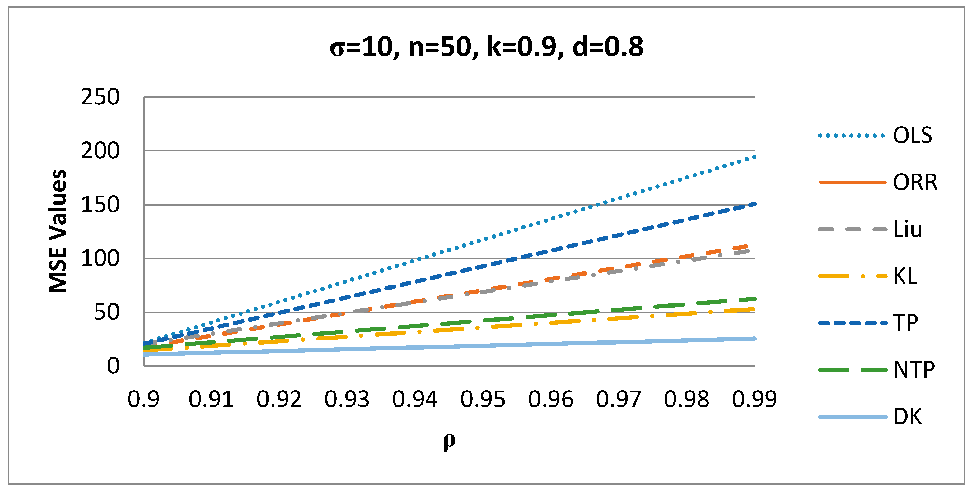
To see the effect of various parameters on MSE, we plotted MSE vs. the parameters in Figure 1, Figure 2, Figure 3, Figure 4, Figure 5 and Figure 6.

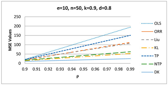
Figure 1. MSE values versus $\rho$ values.

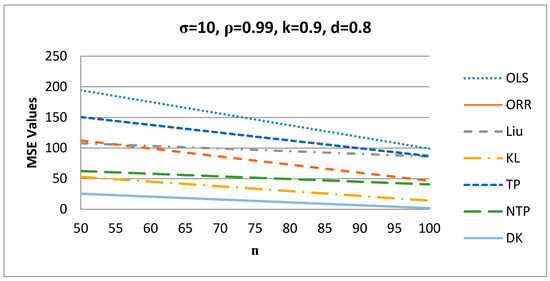
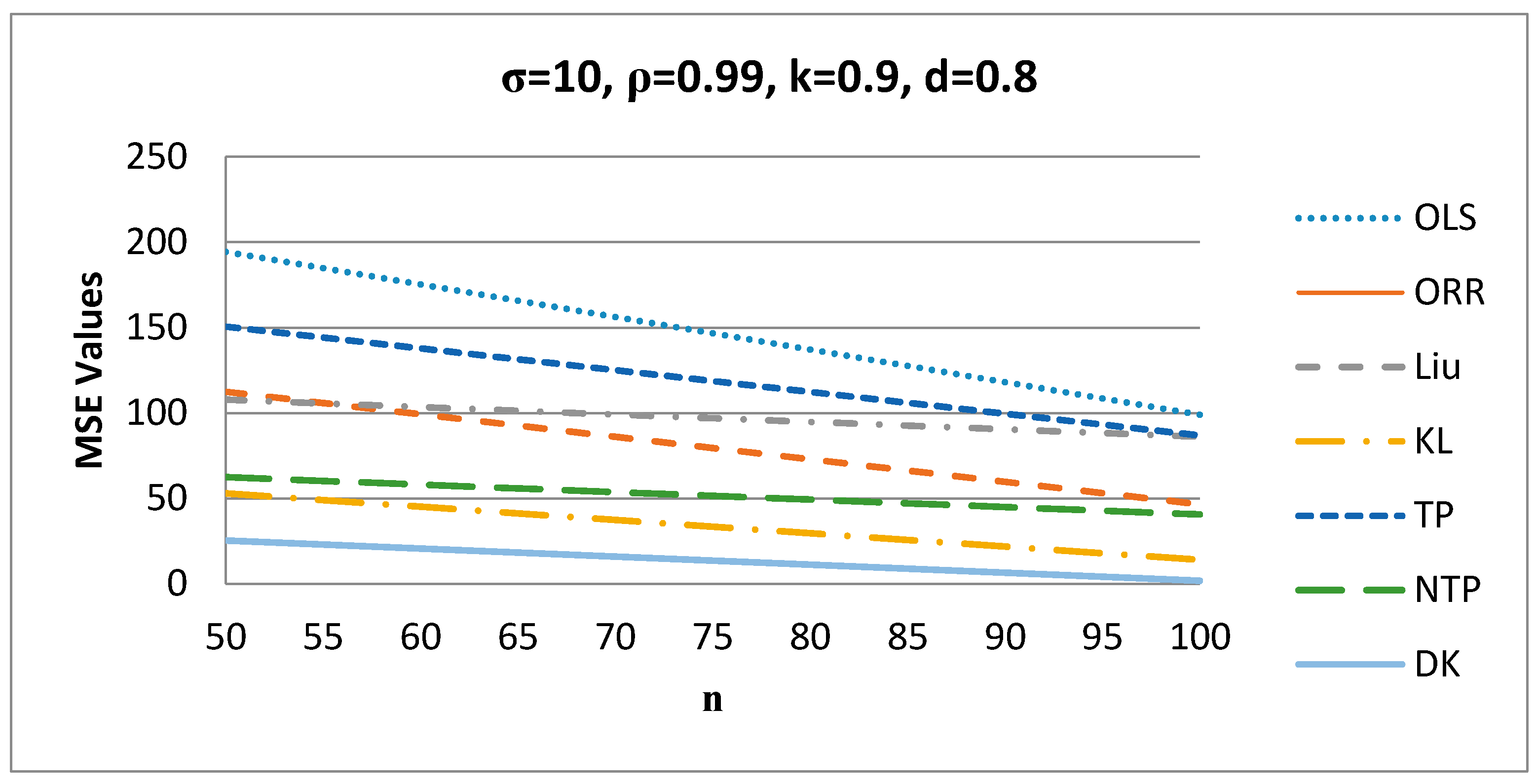
Figure 2. MSE values versus $n$ values.

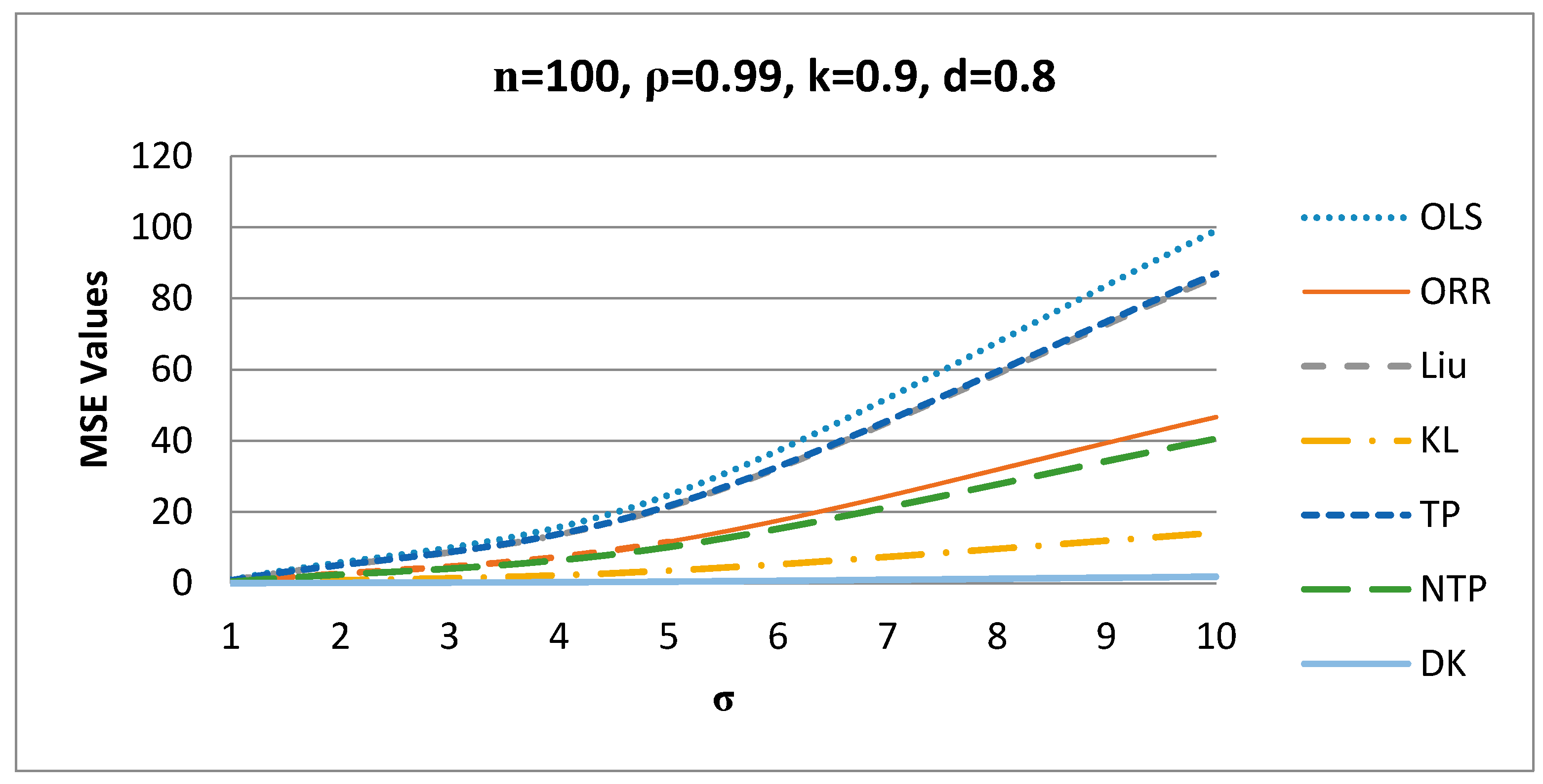
Figure 3. MSE values versus $\sigma$ values.

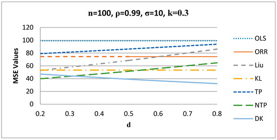
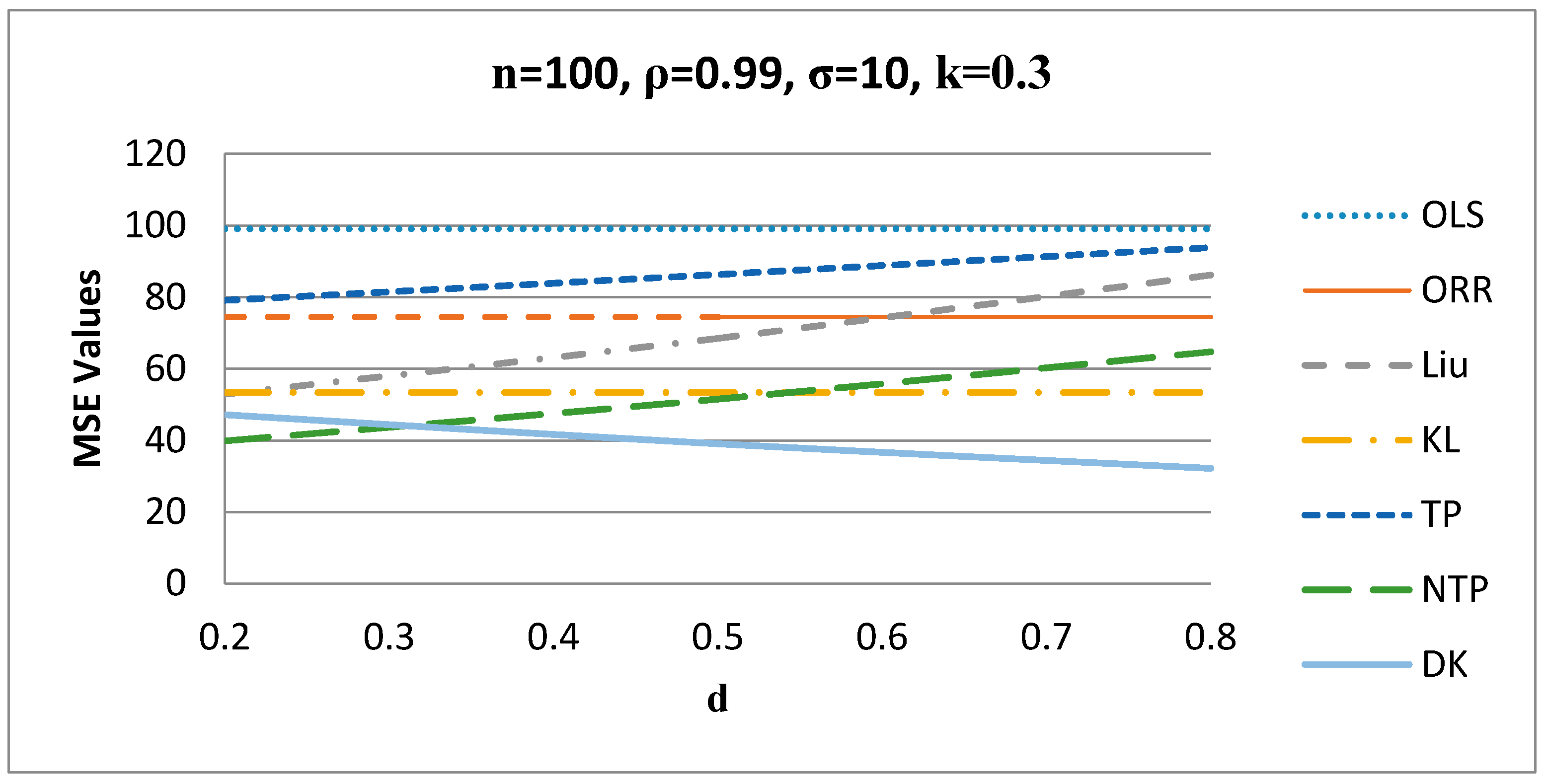
Figure 4. MSE values versus $d$ values when k = 0.3.

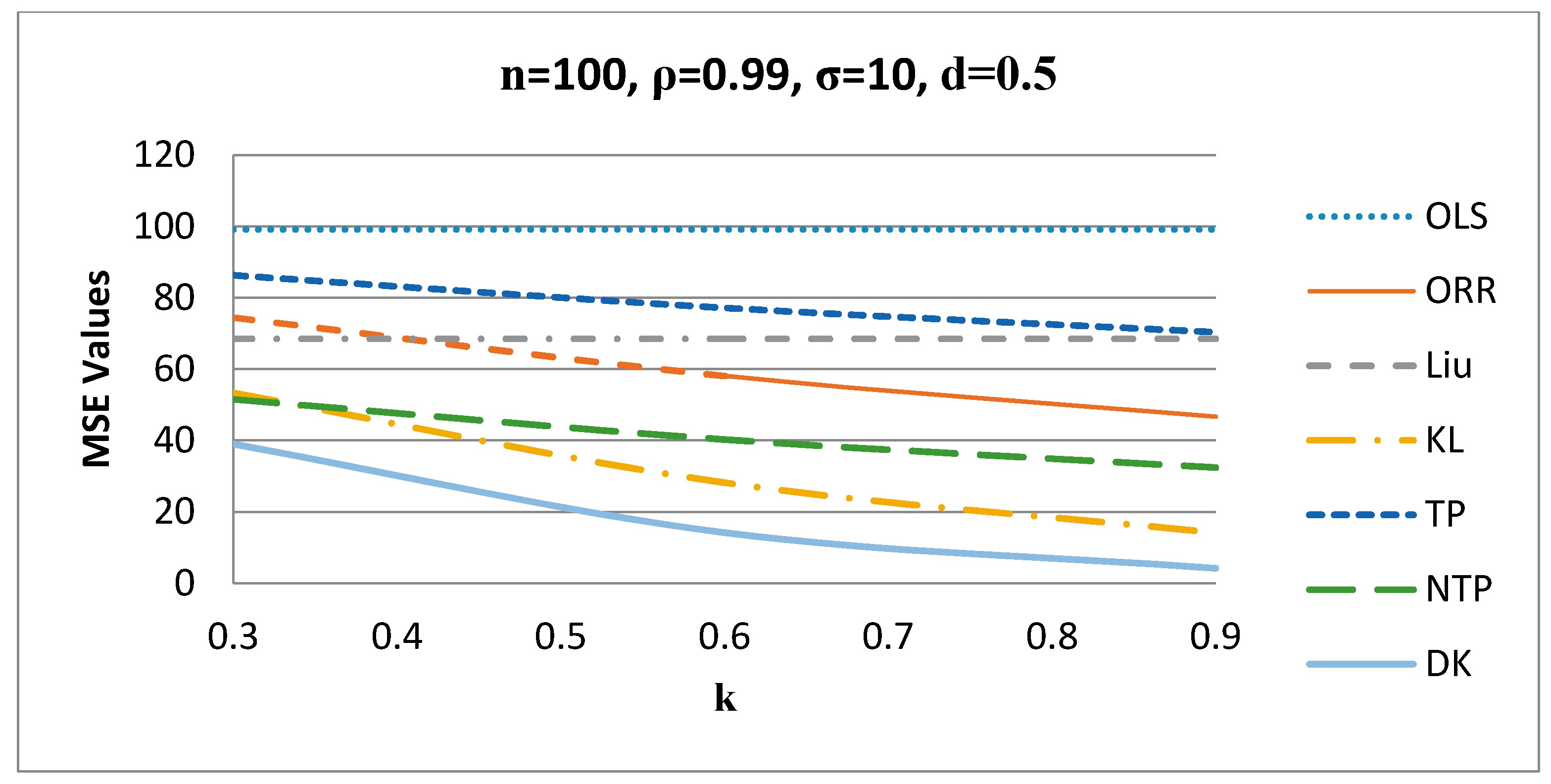
Figure 5. MSE values versus $k$ values when d = 0.5.

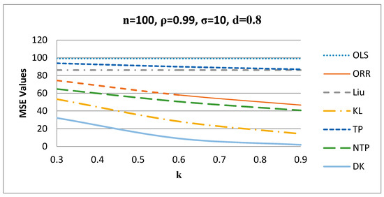
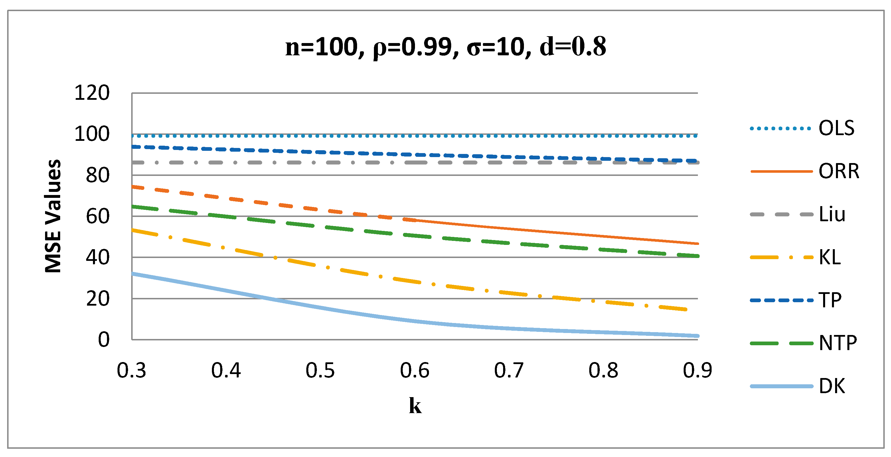
Figure 6. MSE values versus $k$ values when d = 0.8.

It appears from Figure 1 that as $\rho$ increases, the MSE values of the estimators increase for σ = 10, n = 50, k = 0.9, and d = 0.8, and the proposed DK estimator has the smallest MSE value among all estimators.

Figure 2 shows that as $n$ increases, the MSE values of the estimators decrease for σ = 10, ρ = 0.99, k = 0.9, and d = 0.8, and the proposed DK estimator has the smallest MSE value among all estimators.

Figure 3 shows the behavior of $\sigma$, where as $\sigma$ increases, the MSE values of the estimators increase for n = 100, ρ = 0.99, k = 0.9, d = 0.8, and for other values of these factors.

Figure 4 shows the behavior of the estimators for different values of $d$ when $k=0.3$. It is evident from Figure 4 that the proposed DK estimator gives the smallest MSE values when d is greater than 0.3, while the NTP estimator gives better results when d is less than 0.3 for n = 100, ρ = 0.99, σ = 10, and for other values of these factors.

Figure 5 shows the behavior of the estimators for different values of $k$ when $d=0.5$, such that the proposed DK estimator gives the smallest MSE values among all other estimators for n = 100, ρ = 0.99, σ = 10, and for other values of these factors.

Figure 6 shows the behavior of the estimators for different values of $k$ when $d=0.8$, such that the proposed DK estimator gives the smallest MSE values among all other estimators for n = 100, ρ = 0.99, σ = 10, and for other values of these factors.

4. Application

4.1. Portland Cement Data

We use the Portland cement data, which was originally adopted by Woods et al. [29] to explain their theoretical results. The data were analyzed by various researchers: to mention a few, Kaciranlar et al. [30], Li and Yang [31], Lukman et al. [13], and, recently, Kibria and Lukman [15], among others.

The regression model for these data is defined as

$$y_i={\beta }_0+{\beta }_1{X}_1+{\beta }_2{X}_2+{\beta }_3{X}_3+{\beta }_4{X}_4+{\epsilon }_i.$$

(45)

For more details about these data, see Woods et al. [29].

The variance inflation factors are $VI{F}_1=38.50$, $VI{F}_2=254.42$, $VI{F}_3=46.87$, and $VI{F}_4=282.51$. Eigenvalues of $S$ are ${\lambda }_1=44676.206$, ${\lambda }_2=5965.422$, ${\lambda }_3=809.952$, and ${\lambda }_4=105.419$, and the condition number of $S$ is approximately 20.58. The VIFs, the eigenvalues, and the condition number all indicate that severe multicollinearity exists. The estimated parameters and the MSE values of the estimators are presented in Table 5. It appears from Table 5 that the proposed DK estimator performs the best among the mentioned estimators as it gives the smallest MSE value.

Table 5. The results of regression coefficients and the corresponding MSE values.

Coef.	$\widehat{\mathit{\alpha }}$	$\widehat{\mathit{\alpha }}(\widehat{\mathit{k}})$	$\widehat{\mathit{\alpha }}(\widehat{\mathit{d}})$	$\begin{array}{c}{\widehat{\mathit{\alpha }}}_{\mathit{K}\mathit{L}}\\ ({\widehat{\mathit{k}}}_{\mathbf{min}})\end{array}$	$\begin{array}{c}{\widehat{\mathit{\alpha }}}_{\mathit{T}\mathit{P}}\\ (\widehat{\mathit{k}},\widehat{\mathit{d}})\end{array}$	$\begin{array}{c}{\widehat{\mathit{\alpha }}}_{\mathit{N}\mathit{T}\mathit{P}}\\ (\widehat{\mathit{k}},\widehat{\mathit{d}})\end{array}$	$\begin{array}{c}{\widehat{\mathit{\alpha }}}_{\mathit{D}\mathit{K}}\\ ({\widehat{\mathit{k}}}_{\mathbf{min}},{\widehat{\mathit{d}}}_{\mathbf{min}})\end{array}$
${\alpha }_0$	62.405	8.5871	27.665	27.627	32.386	3.8295	27.588
${\alpha }_1$	1.5511	2.1046 *	1.9008 *	1.9088 *	1.8598 *	2.1459 *	1.9092 *
${\alpha }_2$	0.5101	1.0648 *	0.8699 *	0.8685 *	0.8196 *	1.1157 *	0.8689 *
${\alpha }_3$	0.1019	0.6680 *	0.4619	0.4678	0.4177	0.7126 *	0.4682
${\alpha }_4$	−0.1440	0.3995 *	0.2080	0.2072	0.1592	0.4488 *	0.2076
$k$	-----------	0.007676	-	0.000471	0.007676	0.007676	0.000471
$d$	-----------	-----------	0.442224	-----------	0.442224	0.442224	0.001536
$MSE$	4912.090	2989.820	2170.967	2170.9604	2222.682	3450.710	2170.9602

* Coefficient is significant at 0.05.

4.2. Longley Data

Longley data were originally used by Longley [32] and then by other authors (Yasin and Murat [33]; Lukman and Ayinde [22]). The regression model of this data is defined as

$$y={\beta }_1{x}_1+{\beta }_2{x}_2+\dots +{\beta }_5{x}_5+{\beta }_6{x}_6+\epsilon$$

(46)

For more details about these data, see Longley [32].

The variance inflation factors are $VI{F}_1=135.53$, $VI{F}_2=1788.51$, $VI{F}_3=33.62$$VI{F}_4=3.59$, $VI{F}_5=399.15$, and $VI{F}_6=758.98$. Eigenvalues of $S$ are as follows: 2.76779 × 10¹², 7,039,139,179, 11,608,993.96, 2,504,761.021, 1738.356, 13.309, and the condition number of $S$ is approximately 456,070. The VIFs, the eigenvalues, and the condition number all indicate that severe multicollinearity exists. The estimated parameters and the MSE values of the estimators are presented in Table 6. It appears from Table 6 that the proposed DK estimator performs the best among the mentioned estimators as it gives the smallest MSE value.

Table 6. The results of regression coefficients and the corresponding MSE values.

Coef.	$\widehat{\mathit{\alpha }}$	$\widehat{\mathit{\alpha }}(\widehat{\mathit{k}})$	$\widehat{\mathit{\alpha }}(\widehat{\mathit{d}})$	$\begin{array}{c}{\widehat{\mathit{\alpha }}}_{\mathit{K}\mathit{L}}\\ ({\widehat{\mathit{k}}}_{\mathbf{min}})\end{array}$	$\begin{array}{c}{\widehat{\mathit{\alpha }}}_{\mathit{T}\mathit{P}}\\ (\widehat{\mathit{k}},\widehat{\mathit{d}})\end{array}$	$\begin{array}{c}{\widehat{\mathit{\alpha }}}_{\mathit{N}\mathit{T}\mathit{P}}\\ (\widehat{\mathit{k}},\widehat{\mathit{d}})\end{array}$	$\begin{array}{c}{\widehat{\mathit{\alpha }}}_{\mathit{D}\mathit{K}}\\ ({\widehat{\mathit{k}}}_{\mathbf{min}},{\widehat{\mathit{d}}}_{\mathbf{min}})\end{array}$
${\alpha }_1$	−52.994	1.0931	−49.641	−5.0190	−7.7933	1.2529	−5.0188
${\alpha }_2$	0.0711 *	0.0526 *	0.0704 *	0.0609 *	0.0556 *	0.0525 *	0.0609 *
${\alpha }_3$	−0.4235	−0.6457 *	−0.4316	−0.5426	−0.6092 *	−0.6464 *	−0.5427
${\alpha }_4$	−0.5726 *	−0.5611	−0.5745	−0.5985 *	−0.5630	−0.5610	−0.5984 *
${\alpha }_5$	−0.4142	−0.2062	−0.4083	−0.3266	−0.2404	−0.2056	−0.3267
${\alpha }_6$	48.418 *	37.119 *	48.046 *	42.918 *	38.976 *	37.085 *	42.918 *
$k$	---------	262.88	---------	9.5600	262.88	262.88	8.2110
$d$	---------	---------	0.1643	---------	0.1643	0.1643	0.1643
$MSE$	17095	3190.6	15183	2915.1	2945.3	3204.1	2914.7

* Coefficient is significant at 0.05.

5. Summary and Concluding Remarks

In this paper, we introduced a new class of two-parameter estimator, namely, the Dawoud–Kibria (DK) estimator, to solve the multicollinearity problem for linear regression models. We theoretically compared the proposed DK estimator with some existing estimators, for example, the ordinary least squares (OLS) estimator, the ordinary ridge regression (ORR) estimator, the Liu (1993) estimator, the new modified ridge-type estimator of Kibria and Lukman (KL; 2020), the two-parameter (TP) estimator of Ozkale and Kaciranlar (2007), and the new two-parameter (NTP) estimator of Yang and Chang (2010), and derived the biasing parameters $d$ and $k$ of the proposed DK estimator. A simulation study has been conducted to compare the performance of the OLS, ORR, Liu, KL, TP, NTP, and the proposed DK estimators. It is evident from simulation results that the proposed DK estimator gives better results than the rest of the estimators under some conditions. Real-life datasets were analyzed to illustrate the findings of the paper. Hopefully, the paper will be useful for practitioners of various fields.

References

- Hoerl, A.E.; Kennard, R.W. Ridge regression: Biased estimation for nonorthogonal problems. Technometrics 1970, 12, 55–67. [Google Scholar] [CrossRef]
- Stein, C. Inadmissibility of the usual estimator for the mean of a multivariate normal distribution. In Proceedings of the Third Berkeley Symposium on Mathematical Statistics and Probability; MR0084922; University California Press: Berkeley, CA, USA, 1956; Volume 197–206, pp. 1954–1955. [Google Scholar]
- Massy, W.F. Principal components regression in exploratory statistical research. J. Am. Stat. Assoc. 1965, 60, 234–256. [Google Scholar] [CrossRef]
- Mayer, L.S.; Willke, T.A. On biased estimation in linear models. Technometrics 1973, 15, 497–508. [Google Scholar] [CrossRef]
- Swindel, B.F. Good ridge estimators based on prior information. Commun. Stat. Theory Methods 1976, 5, 1065–1075. [Google Scholar] [CrossRef]
- Liu, K. A new class of biased estimate in linear regression. Commun. Stat. Theory Methods 1993, 22, 393–402. [Google Scholar]
- Akdeniz, F.; Kaçiranlar, S. On the almost unbiased generalized liu estimator and unbiased estimation of the bias and mse. Commun. Stat. Theory Methods 1995, 24, 1789–1797. [Google Scholar] [CrossRef]
- Ozkale, M.R.; Kaçiranlar, S. The restricted and unrestricted two-parameter estimators. Commun. Stat. Theory Methods 2007, 36, 2707–2725. [Google Scholar] [CrossRef]
- Sakallıoglu, S.; Kaçıranlar, S. A new biased estimator based on ridge estimation. Stat. Pap. 2008, 49, 669–689. [Google Scholar] [CrossRef]
- Yang, H.; Chang, X. A new two-parameter estimator in linear regression. Commun. Stat. Theory Methods 2010, 39, 923–934. [Google Scholar] [CrossRef]
- Roozbeh, M. Optimal QR-based estimation in partially linear regression models with correlated errors using GCV criterion. Comput. Stat. Data Anal. 2018, 117, 45–61. [Google Scholar] [CrossRef]
- Akdeniz, F.; Roozbeh, M. Generalized difference-based weighted mixed almost unbiased ridge estimator in partially linear models. Stat. Pap. 2019, 60, 1717–1739. [Google Scholar] [CrossRef]
- Lukman, A.F.; Ayinde, K.; Binuomote, S.; Clement, O.A. Modified ridge-type estimator to combat multicollinearity: Application to chemical data. J. Chemother. 2019, 33, e3125. [Google Scholar] [CrossRef]
- Lukman, A.F.; Ayinde, K.; Sek, S.K.; Adewuyi, E. A modified new two-parameter estimator in a linear regression model. Model. Eng. Simul. 2019, 2019, 6342702. [Google Scholar] [CrossRef]
- Kibria, B.M.G.; Lukman, A.F. A New Ridge-Type Estimator for the Linear Regression Model: Simulations and Applications. Hindawi Sci. 2020, 2020, 9758378. [Google Scholar] [CrossRef]
- Wang, S.G.; Wu, M.X.; Jia, Z.Z. Matrix Inequalities; Science Chinese Press: Beijing, China, 2006. [Google Scholar]
- Farebrother, R.W. Further results on the mean square error of ridge regression. J. R. Stat. Soc. B 1976, 38, 248–250. [Google Scholar] [CrossRef]
- Trenkler, G.; Toutenburg, H. Mean squared error matrix comparisons between biased estimators-an overview of recent results. Stat. Pap. 1990, 31, 165–179. [Google Scholar] [CrossRef]
- Hoerl, A.E.; Kannard, R.W.; Baldwin, K.F. Ridge regression: Some simulations. Commun. Stat. 1975, 4, 105–123. [Google Scholar] [CrossRef]
- Kibria, B.M.G. Performance of some new ridge regression estimators. Commun. Stat. Simul. Comput. 2003, 32, 419–435. [Google Scholar] [CrossRef]
- Kibria, B.M.G.; Banik, S. Some ridge regression estimators and their performances. J. Mod. Appl. Stat. Methods 2016, 15, 206–238. [Google Scholar] [CrossRef]
- Lukman, A.F.; Ayinde, K. Review and classifications of the ridge parameter estimation techniques. Hacet. J. Math. Stat. 2017, 46, 953–967. [Google Scholar] [CrossRef]
- Månsson, K.; Kibria, B.M.G.; Shukur, G. Performance of some weighted Liu estimators for logit regression model: An application to Swedish accident data. Commun. Stat. Theory Methods 2015, 44, 363–375. [Google Scholar] [CrossRef]
- Khalaf, G.; Shukur, G. Choosing ridge parameter for regression problems. Commun. Stat. Theory Methods 2005, 21, 2227–2246. [Google Scholar] [CrossRef]
- Gibbons, D.G. A simulation study of some ridge estimators. J. Am. Stat. Assoc. 1981, 76, 131–139. [Google Scholar] [CrossRef]
- Newhouse, J.P.; Oman, S.D. An evaluation of ridge estimators. In A Report Prepared for United States Air Force Project; RAND: Santa Monica, CA, USA, 1971. [Google Scholar]
- Wichern, D.W.; Churchill, G.A. A comparison of ridge estimators. Technometrics 1978, 20, 301–311. [Google Scholar] [CrossRef]
- Kan, B.; Alpu, O.; Yazıcı, B. Robust ridge and robust Liu estimator for regression based on the LTS estimator. J. Appl. Stat. 2013, 40, 644–655. [Google Scholar] [CrossRef]
- Woods, H.; Steinour, H.H.; Starke, H.R. Effect of composition of Portland cement on heat evolved during hardening. J. Ind. Eng. Chem. 1932, 24, 1207–1214. [Google Scholar] [CrossRef]
- Kaciranlar, S.; Sakallioglu, S.; Akdeniz, F.; Styan, G.P.H.; Werner, H.J. A new biased estimator in linear regression and a detailed analysis of the widely-analysed dataset on portland cement. Sankhya Indian J. Stat. B 1999, 61, 443–459. [Google Scholar]
- Li, Y.; Yang, H. Anew Liu-type estimator in linear regression model. Stat. Pap. 2012, 53, 427–437. [Google Scholar] [CrossRef]
- Longley, J.W. An appraisal of least squares programs for electronic computer from the point of view of the user. J. Am. Stat. Assoc. 1967, 62, 819–841. [Google Scholar] [CrossRef]
- Yasin, A.; Murat, E. Influence Diagnostics in Two-Parameter Ridge Regression. J. Data Sci. 2016, 14, 33–52. [Google Scholar]
Publisher’s Note: MDPI stays neutral with regard to jurisdictional claims in published maps and institutional affiliations. |
© 2020 by the authors. Licensee MDPI, Basel, Switzerland. This article is an open access article distributed under the terms and conditions of the Creative Commons Attribution (CC BY) license (http://creativecommons.org/licenses/by/4.0/).