Article

An Upper Bound of the Bias of Nadaraya-Watson Kernel Regression under Lipschitz Assumptions

1
Computer Science Department, Technische Universität Darmstadt, 64289 Darmstadt, Germany
2
Computer Science Department, Max Planck Institute for Intelligent Systems, 70569 Stuttgart, Germany
*
Author to whom correspondence should be addressed.
Stats 2021, 4(1), 1-17; https://doi.org/10.3390/stats4010001
Submission received: 30 October 2020 / Revised: 12 December 2020 / Accepted: 25 December 2020 / Published: 30 December 2020
(This article belongs to the Section Regression Models)

Abstract

:
The Nadaraya-Watson kernel estimator is among the most popular nonparameteric regression technique thanks to its simplicity. Its asymptotic bias has been studied by Rosenblatt in 1969 and has been reported in several related literature. However, given its asymptotic nature, it gives no access to a hard bound. The increasing popularity of predictive tools for automated decision-making surges the need for hard (non-probabilistic) guarantees. To alleviate this issue, we propose an upper bound of the bias which holds for finite bandwidths using Lipschitz assumptions and mitigating some of the prerequisites of Rosenblatt’s analysis. Our bound has potential applications in fields like surgical robots or self-driving cars, where some hard guarantees on the prediction-error are needed.

1. Introduction

Nonparametric regression and density estimation have been used in a wide spectrum of applications, ranging from economics [1], system dynamics identification [2,3], and reinforcement learning [4,5,6,7]. In recent years, nonparametric density estimation and regression have been dominated by parametric methods such as those based on deep neural networks. These parametric methods have demonstrated an extraordinary capacity in dealing with both high-dimensional data—such as images, sounds, or videos—and large datasets. However, it is difficult to obtain strong guarantees on such complex models, which have been shown easy to fool [8]. Nonparametric techniques have the advantage of being easier to understand, and recent work overcame some of their limitations by, e.g., allowing linear-memory and sub-linear query time for density kernel estimation [9,10]. These methods allowed nonparametric kernel density estimation to be performed on datasets of 10 6 samples and up to 784 input dimension. As such, nonparametric methods are a suitable choice when one is willing to trade performance for statistical guarantees; and the contribution of this paper is to advance the state-of-the-art on such guarantees.
Studying the error of a statistical estimator is important. It can be used, for example, to tune the hyper-parameters by minimizing the estimated error [11,12,13,14]. To this end, the estimation error is usually decomposed into an estimation bias and variance. When it is not possible to derive these quantities, one performs an asymptotic behavior analysis or a convergence to a probabilistic distribution of the error. While all aforementioned analyses give interesting insights on the error and allow for hyper-parameter optimization, they do not provide any strong guarantee on the error, i.e., we cannot upper bound it with absolute certainty.
Beyond hyper-parameter optimization, we argue that another critical aspect of error analysis is to provide hard (non-probabilistic) bounds of the error for critical data-driven algorithms. We believe that learning agents taking autonomous, data-driven, decisions will be increasingly present in the near future. These agents will, for example, be autonomous surgeons, self-driving cars or autonomous manipulators. In many critical applications involving these agents, it is of primary importance to bound the prediction error in order to provide some technical guarantees on the agent’s behavior. In this paper we derive a hard upper bound of the estimation bias in non-parametric regression with minimal assumptions on the problem. The bound can be readily applied to a wide range of applications.
Specifically, we consider the Nadaraya-Watson kernel regression [15,16], which can be seen as a conditional kernel density estimate. We derive an upper bound of the estimation bias under weak local Lipschitz assumptions. The reason for our choice of estimator falls in its inherent simplicity compared to more sophisticated techniques. The bias of the Nadaraya-Watson kernel regression has been previously studied by [17], and has been reported in a number of related work [18,19,20,21]. The analysis of the bias conducted by Rosenblatt (1969) [17] still remains the main reference for this regression technique. The main assumptions of Rosenblatt’s analysis are h n 0 (where n is the number of samples) and n h n where h n is the kernel’s bandwidth. Rosenblatt’s analysis suffers from an asymptotic error o ( h n 2 ) , which means that for large bandwidths it is not accurate; making it inapplicable to derive a hard upper bound. To the best of our knowledge, the only proposed bound on the bias requires the restrictive assumption that the samples must be placed evenly on a closed interval [22]. In contrast, we derive an upper bound of the bias of the Nadaraya-Watson kernel regression that is valid for a large class of design and for any choice of bandwidth.
We build our analysis on weak Lipschitz assumptions [23], which are milder than the (global) Lipschitz, as we require only | f ( x ) f ( y ) | L | x y |   y C given a fixed x, instead of the classic | f ( x ) f ( y ) | L | x y |   y , x C —where C is the data domain. Lipschitz assumptions are common in different fields, and usually allow a wide family of admissible functions. This is particularly true when the Lipschitz is require for only a subset of the function’s domain (like in our case). Moreover, notice that the classical analysis requires the knowledge of the second derivative of the regression function m, and therefore the continuity of m . Our Lipschitz assumption is less restrictive, allowing us to obtain a bias upper bound even for functions like m ( x ) = | x | , at points (like x = 0 ) where m is undefined. The Rosenblatt analysis builds on a Taylor expansion of the estimator and therefore when the bandwidth h n is large, Rosenblatt’s bias analysis tends to provide wrong estimates of the bias, as observed in the experimental section. We consider multidimensional input space, and we apply the bound to a realistic regression problem.

2. Preliminaries

Consider the problem of estimating E [ Y | X = x ] where X f X and Y = m ( X ) + ε , with noise ε , i.e., E [ ε ] = 0 . The noise can depend on x , but since our analysis is conducted point-wise for a given x , ε x will be simply denoted by ε . Let m : R d R be the regression function and f X a probability distribution on X called design. In our analysis we consider X R d and Y R . The Nadaraya-Watson kernel estimate of E [ Y | X = x ] is
m ^ ( x ) = i = 1 n K h ( x x i ) y i j = 1 n K h ( x x j ) ,
where K h is a kernel function with bandwidth-vector h , the x i are drawn from the design f X and y i from m ( x i ) + ε . Note that both the numerator and the denominator are proportional to Parzen-Rosenblatt density kernel estimates [24,25]. We are interested in the point-wise bias of such estimate E [ m ^ ( x ) ] m ( x ) . In the prior analysis of [17], knowledge of m , m , f X , f X is required and f , m must be continuous in a neighborhood of x. In addition, and as discussed in the introduction, the analysis is limited to a one-dimensional design and an infinitesimal bandwidth. We briefly present the classical bias analysis of [17] before introducing our results for clarity of exposition.
Theorem 1.
Classic Bias Estimation [17]. Let m : R R be twice differentiable. Assume a set { x i , y i } i = 1 n , where x i are i.i.d. samples from a distribution with non-zero differentiable density f X . Assume y i = m ( x i ) + ε i , with noise ε i ε ( x i ) . The bias of the Nadaraya-Watson kernel in the limit of infinite samples and for h 0 and n h n is
E lim n m ^ n ( x ) m ( x ) = h n 2 1 2 m ( x ) + m ( x ) f X ( x ) f X ( x ) u 2 K ( u ) d u + o P h n 2 h n 2 1 2 m ( x ) + m ( x ) f X ( x ) f X ( x ) u 2 K ( u ) d u .
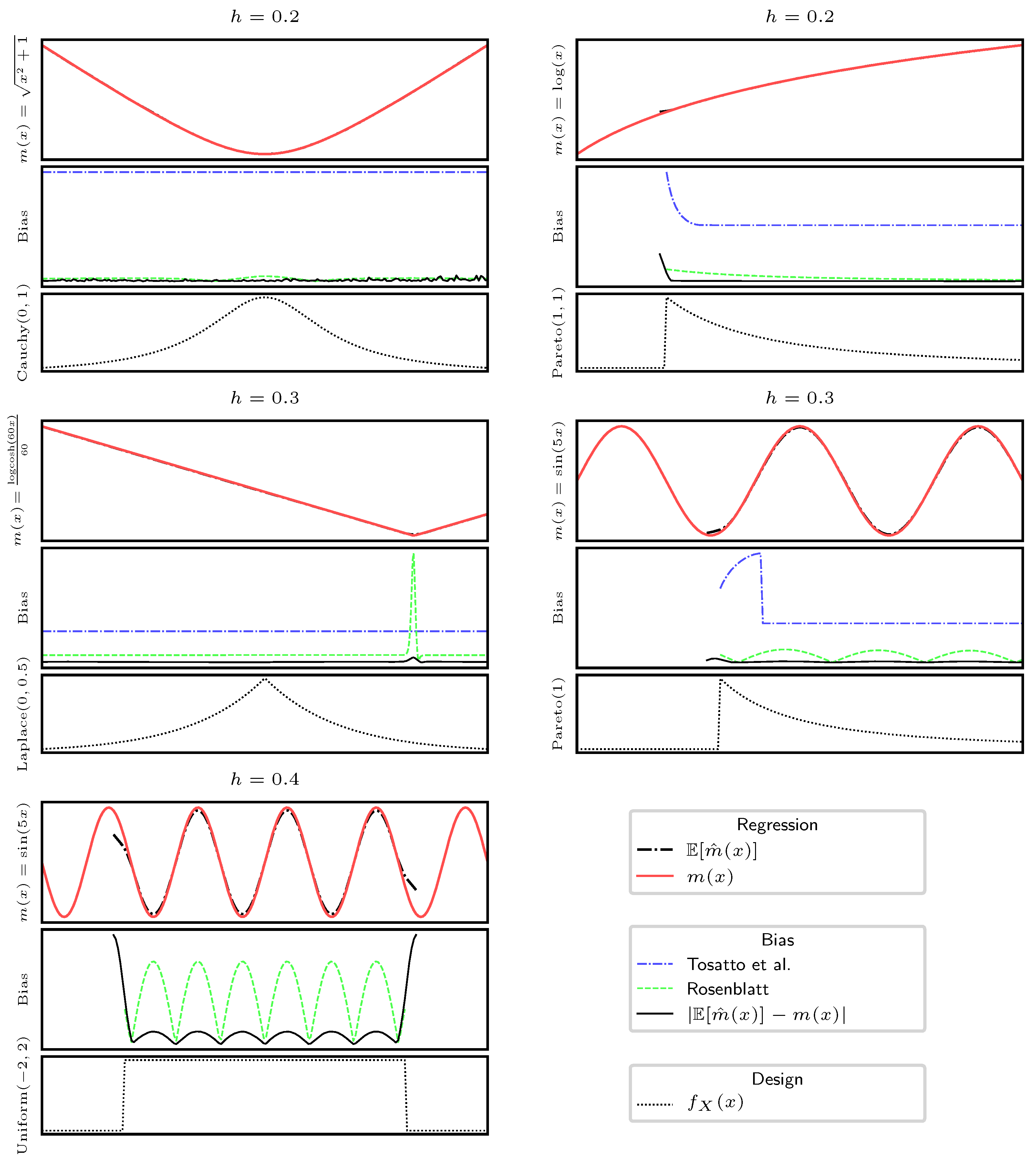
Note that Equation (2) must be normalized with k ( u ) d u when the kernel function does not integrate to one. The o P term denotes the asymptotic behavior w.r.t. the bandwidth. Therefore, for a larger value of the bandwidth, the bias estimation becomes worse, as is illustrated in Figure 1.

3. Main Result

In this section, we present two bounds on the bias of the Nadaraya-Watson estimator. The first one considers a bounded regression function m (i.e., | m ( x ) | M ), and allows for weak Lipschitz conditions on a subset of the design’s support. Instead, the second bound does not require the regression function to be bounded but only the weak Lipschitz continuity to hold on all of its support. The definition of “weak” Lipschitz continuity will be given below.
To develop our bound on the bias for multidimensional inputs is essential to define some subset of the R d space. In more detail, we consider an open n-dimensional interval in R d which is defined as Ω ( τ , τ + ) ( τ 1 , τ 1 + ) × × ( τ d , τ d + ) where τ , τ + R ¯ d . We now formalize what is meant by weak (log-)Lipschitz continuity. This will prove useful as we need knowledge of the weak-Lipschitz constants of m and log f X in our analysis.
Definition 1.
Weak Lipschitz continuity at x on the set C under the L 1 -norm.
Let C R d and f : C R . We call f weak Lipschitz continuous at x C if and only if
| f ( x ) f ( y ) | L | x y | y C ,
where | · | denotes the L 1 -norm.
Definition 2.
Weak log-Lipschitz continuity at x on the set C under the L 1 -norm.
Let C R d . We call f weak log-Lipschitz continuous at x on the set C if and only if
| log f ( x ) log f ( y ) | L | x y | y C .
Note that the set C can be a subset of the function’s domain.
It is important to note that, in contrast to the global Lipschitz continuity, which requires | f ( y ) f ( z ) | L | y z |   y , z C , the weak Lipschitz continuity is defined at a specific point x and therefore allows the function to be discontinuous elsewhere. The Lipschitz assumptions are not very restrictive, and in practice require a bounded gradient. They have been widely used in various fields. Note that when the Lipschitz constants are not known, they can be estimated from the dataset [26]. In the following we list the set of assumptions that we use in our theorems.
A1. 
f X and m are defined on Y Ω ( x υ , x + υ + ) and υ , υ + R ¯ + d ;
A2. 
f X is log weak Lipschitz with constant L f at x on the set D Ω ( x δ , x + δ ) Y and f X ( x ) f X ( z )   z Y \ D with positive defined δ , δ + R ¯ + d (note that this implies f X ( y ) > 0   y D );
A3. 
m is weak Lipschitz with constant L m at x on a the set G Ω ( x γ , x + γ + ) D with positive defined γ , γ + R ¯ + d .
To work out a bound on the bias valid for a wide class of kernels, we must enumerate some assumption and quantify some integrals with respect to the kernel.
A4. 
The multidimensional kernel K h : R d R can be decomposed in a product of independent uni-dimensional kernels, i.e., K h ( x ) = i = 1 d k i ( x / h i ) with k i : R R ;
A5. 
the kernels are non-negative k i ( x ) 0 and symmetric k i ( x ) = k i ( x ) ;
A6. 
for every a , x R and h 0 , the integrals 0 a k i ( x ) d x = Φ i ( a ) , 0 a k i ( x ) e x L f d x = B i ( x , L f ) , 0 a k i ( x ) x e x L f d x = C i ( x , L f ) are finite (i.e., < + ).
Assumptions A4–A6 are not really restrictive, and includes any kernel with both finite domain and co-domain, or not heavy-tailed (e.g., Gaussian-like). Furthermore, Axiom A4 allows any independent composition of different kernel functions. In Appendix B we detail the integrals of Axiom A6 for different kernels. Note that when the integrals listed in A6 exist in closed form, the computation of the bound is straightforward, and requires negligible computational effort.
In the following, we propose two different bounds of the bias. The first version considers a bounded regression function ( M < + ), this allows both the regression function and the design to be weak Lipschitz on a subset of their domain. In the second version instead, we consider the case of an unbounded regression function ( M = + ) or an unknown bound M. In this case both the regression function and the design must be weak Lipschitz on the entire domain Y .
Theorem 2.
Bound on the Bias with Bounded Regression Function.
Assuming A1–A3, h R + d a positive defined vector of bandwidths h = [ h 1 , h 2 , , h n ] , K h the multivariate kernel defined in A4–A6, m ^ n ( x ) the Nadaraya-Watson kernel estimate using n observations { x i , y i } i = 1 n with x i f X , y i = m ( x i ) + ε i and with noise ε i ε ( x i ) centered in zero ( E [ ε ( x i ) ] = 0 ), n , and furthermore assuming there is a constant 0 M < + such that | m ( y ) m ( z ) | M   y , z Y , the considered Nadaraya-Watson kernel regression bias is bounded by
| E lim n m ^ n ( x ) m ( x ) | L m k = 1 d ξ k ( ϕ k , ϕ k + ) i k d ζ ( ϕ i , ϕ i + ) + M i = 1 d ζ ( γ i , γ i + ) i = 1 d ζ ( ϕ i , ϕ i + ) + D i = 1 d ψ i ( δ i , δ i + )
where
ψ i ( a , b ) = h i B i ( b / h i , L f h i ) B i ( a / h i , L f h i ) , ζ i ( a , b ) = h i B i ( b / h i , L f h i ) B i ( a / h i , L f h i ) , ξ i ( a , b ) = h i 2 C i ( b / h i , L f h i ) + C i ( a h i , L f h i ) , D = lim ω + i = 1 d h i Φ i ω h i i = 1 d h i φ i ,
with φ i = Φ i ( γ i + / h i ) + Φ i ( γ i / h i ) , and 0 < ϕ i γ i , 0 < ϕ i + γ i + can be freely chosen to obtain a tighter bound. We suggest ϕ i + = min ( γ i + , M / L m ) , ϕ i = min ( γ i , M / L m ) .
In the case where M is unknown or infinite, we propose the following bound.
Theorem 3.
Bound on the Bias with Unbounded Regression Function.
Assuming A1–A3, h R ¯ + d a positive defined vector of bandwidths h = [ h 1 , h 2 , , h n ] , K h the multivariate kernel defined in A4–A6, m ^ n ( x ) the Nadaraya-Watson kernel estimate using n observations { x i , y i } i = 1 n with x i f X , y i = m ( x i ) + ε i and with noise ε i ε ( x i ) centered in zero ( E [ ε ( x i ) ] = 0 ), n , and furthermore assuming that Y D G , the considered Nadaraya-Watson kernel regression bias is bounded by
| E lim n m ^ n ( x ) m ( x ) | L m k = 1 d ξ k ( υ k , υ k + ) i k d ζ i ( υ i , υ i + ) i = 1 d ψ i ( υ i , υ i + ) ,
where ξ k , ζ i , ψ i are defined as in Theorem 2.
We detail the proof of both theorems in Appendix A. Note that the conditions required by our theorems are mild, and they allow a wide range of random designs, including and not limited to Gaussian, Cauchy, Pareto, Uniform, and Laplace distributions. In general, every continuously differentiable density distribution is also weak log-Lipschitz in some closed subset of its domain. For example, the Gaussian distribution does not have a finite Lipschitz constant on its entire domain, but there is a finite weak Lipschitz constant on any closed interval. Examples of distributions that are weak log-Lipschitz are presented in Table 1.

4. Analysis

Although the bound applies to different kernel functions, in the following we analyze the most common Gaussian kernel. It worth noting that for k ( x ) = e x 2 ,
ϕ ( x ) = π 2 erf ( a ) , B ( a , c ) = π 2 e c 2 4 erf a + c 2 erf c 2 , C ( a , c ) = 1 2 1 e a ( a + c ) c B ( a , c ) .
Note that we removed the subscripts from the functions ψ , B, and C, as we consider only the Gaussian kernel. To provide a tight bound, we consider many quantities that describe the design’s domain, the Lipschitz constants of the design and of the regression function, the bound of the image of the regression function, and the different bandwidths for each dimension of the space. This complexity results in an effective but poorly readable bound. In this section, we try to simplify the problem and to analyze the behavior of the bound in the limit.
Asymptotic Analysis: Let us consider, for the moment, the case of one-dimension ( d = 1 ) and infinite domains and co-domains (M unknown and υ = υ + = δ = δ + = γ = γ + = ). In this particular case, the bound becomes
| E lim n m ^ n ( x ) m ( x ) | L m h 1 2 π exp L f 2 h 2 4 + h L f erf h L f 2 + 1 = A 1 .
As expected, for h 0 or for L m = 0 , B 1 = 0 . This result is in line with (2) (since L m = 0 m = 0 ,   m = 0 ). A completely flat design, e.g., uniformly distributed, does not imply a zero bias. This can be seen either in Rosenblatt’s analysis or by just considering the fact that, notoriously, the Nadaraya-Watson estimator suffers from the boundary bias. When we analyze our bound, we find in fact that lim L f 0 B 1 L m h . It is also interesting to analyze the asymptotic behavior when these quantities tend to infinity. Similarly to (2), we observe that A 1 grows quadratically w.r.t. the kernel’s bandwidth h and it scales linearly w.r.t. the Lipschitz constant of the regression function (which is linked to m ). A further analysis brings us to the consideration that Rosenbatt’s analysis is linear w.r.t. d / d x log f X ( x ) (since f X ( x ) / f X ( x ) = d / d x log f X ( x ) ). Our bound has a similar implication, as the Log-Lipschitz constant is also related to the derivative of the logarithm of the design function, and A 1 = O ( L f ) .
Boundary Bias: The Nadaraya-Watson kernel estimator is affected by the boundary bias. The boundary bias is an additive bias term affecting the estimation in the region close to the boundaries of the design’s domains. Since in our framework, we can consider a closed domain of the design, we can also see what is happening close to the border. Let us consider still a one-dimensional regression, but this time υ 0 , υ = δ = γ and υ + = δ + = γ + = . In this case, we obtain
| E lim n m ^ n ( x ) m ( x ) | L m h π e L f 2 h 2 4 1 erf h L f 2 + L m L f h 2 1 + erf h L f 2 2 2 erf h L f 2 = A 2 .
Keeping in account that d / d x erf ( x ) e x and using L’Hôpital’s rule, we can observe that the bound is now exponential w.r.t. h and L f , i.e., A 2 = O ( e h L f ) , which implies that it is more “sensible” to higher bandwidths or less smooth design. Interestingly, instead, the bounds maintains its linear relation w.r.t. L m .
Dimensionality: Let us now study the multidimensional case, supposing that each dimension has same bandwidth and same values for the boundaries. In this case,
| E lim n m ^ n ( x ) m ( x ) | d ξ ( υ , υ + ) ζ ( υ , υ + ) d 1 ψ ( υ , υ + ) d d ζ ( υ , υ + ) ψ ( υ , υ + ) d 1 .
Therefore, the bound scales exponentially w.r.t. the dimension. We observe an exponential behavior when x is close to the boundary of the design’s domain. In these regions, in fact the ratio ζ ( υ , υ + ) / ψ ( υ , υ + ) is particularly high. Of course, when the aforementioned ratio tends to one, the linearity w.r.t. d is predominant.
We can conclude the analysis by noticing that our bound has similar limiting behavior with the Rosenblatt’s analysis, but it provides a hard bound on the bias.

5. Numerical Simulation

In this section, we provide three numerical analyses of our bounds on the bias (the code of our numerical simulations can be found at http://github.com/SamuelePolimi/UpperboundNWBias). The first analysis of our method is conducted on uni-dimensional input spaces for display purposes and aims to show the properties of our bounds in different scenarios. The second analysis aims instead at testing the behavior of our method on a multidimensional input space. The third analysis emulates a realistic scenario where our bound can be applied.
Uni-dimensional Analysis: We select a set of regression functions with different Lipschitz constants and different bounds,
  • y = sin ( 5 x ) ; L m = 5 and M = 1 ,
  • y = log x which for G Ω ( 1 , + ) has L m = 1 and M = + ,
  • y = 60 1 log cosh 60 x which has L m = 1 , is unbuounded, and has a particularly high second derivative in x = 0 , with m ( 0 ) = 60 ,
  • y = x 2 + 1 which has L m = 1 and is unbounded.
A zero-mean Gaussian noise with standard deviation σ = 0.05 has been added to the output y. Our theory applies to a wide family of kernels. In this analysis we consider a Gaussian kernel, with k ( x ) = e x 2 , a box kernel, with k ( x ) = I ( x ) , and a triangle kernel, with k ( x ) = I ( x ) ( 1 | x | ) with
I ( x ) = 1 if | x | 1 , 0 otherwise .
We further analyze the aforementioned kernels in Appendix B. In order to provide as many different scenarios as possible we also used the distributions from Table 1, using therefore both infinite domain distributions, such as Cauchy and Laplace, and finite domain such as Uniform. In order to numerically estimate the bias, we approximate E [ m ^ n ( x ) ] with an ensemble of estimates N 1 j = 1 N m ^ n , j ( x ) where each estimate m ^ n , j is built on a different dataset (drawn from the same distribution f X ). In order to “simulate” n we used n = 10 5 samples, and to obtain high confidence of the bias’ estimate, we used N = 100 models.
In this section we provide some simulations of our bound presented in Theorems 2 and 3, and for the Rosenblatt’s case we use
h n 2 1 2 m ( x ) + m ( x ) f X ( x ) f X ( x ) u 2 K ( u ) d u .
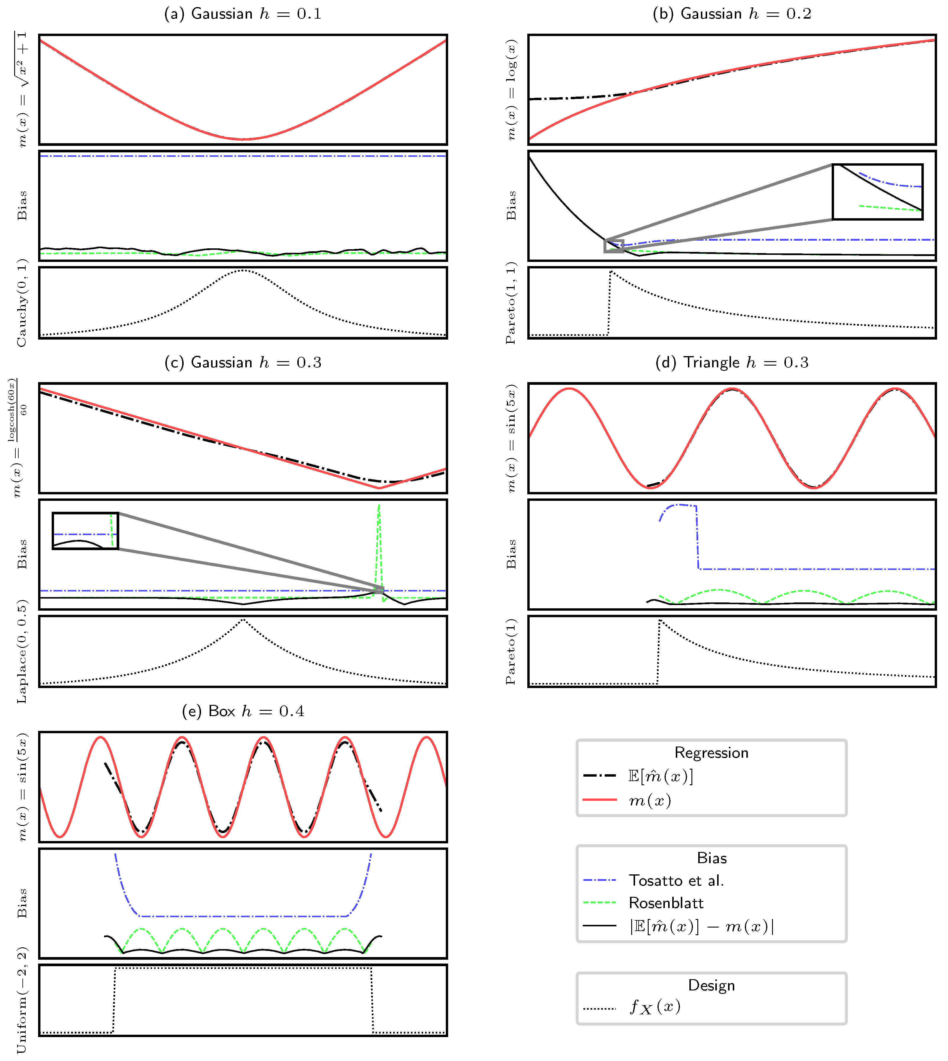
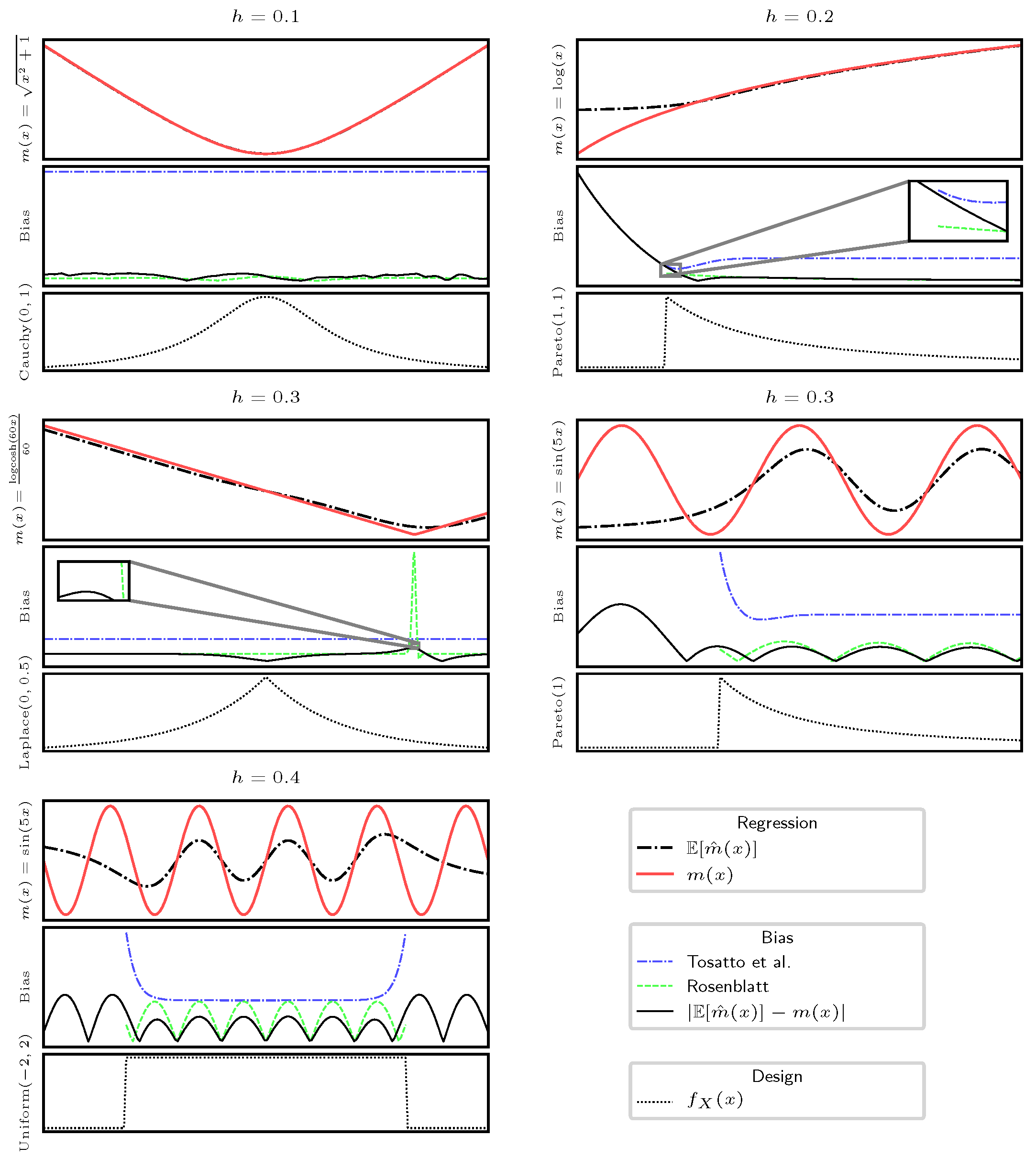
Since the Rosenblatt’s bias estimate is not an upper bound, it can happen that the true bias is higher (as well as lower) than this estimate, as it is possible to see in Figure 1. We presented different scenarios, both with bounded and unbounded functions, infinite and finite design domains, and a larger or smaller bandwidth choice. It is possible to observe that, thanks to the knowledge of f , f , m , m the Rosenblatt’s estimation of the bias tends to be more accurate than our bound. However, it can happen that it largely overestimates the bias, like in the case of m ( x ) = 60 1 log cosh ( 60 x ) in x = 0 or to underestimate it, most often in boundary regions. In contrast, our bound always overestimates the true bias, and despite its lack of knowledge of f , f , m , m , it is most often tight. Moreover, when the bandwidth is small, both our method and Rosenblatt’s deliver an accurate estimation of the bias. In general, Rosenblatt tends to deliver a better estimate of the bias, but it does not behave as a bound, and in some situations, it also can deliver larger mispredictions. In detail, the plot (a) in Figure 1 shows that with a tight bandwidth, both our method and Rosenblatt’s method achieve good approximations of the bias, but only our method correctly upper bounds the bias. When increasing the bandwidth, we obtain both a larger bias and subsequent larger estimates of the bias. Our method consistently upper bounds the bias, while in many cases, Rosenblatt’s method underestimates it, especially in proximity of boundaries (subplots b, d, e). An interesting case can be observed in subplot (c), where we test the function m ( x ) = 60 1 log cosh ( 60 x ) , which has a high second-order derivative in x = 0 : in this case, Rosenblatt’s method largely overestimates the bias.
The figure shows that our bound can deal with different functions and random designs, being reasonably tight, if compared to Rosenblatt’s estimation, which requires the knowledge of the regression function and the design, and respective derivatives.
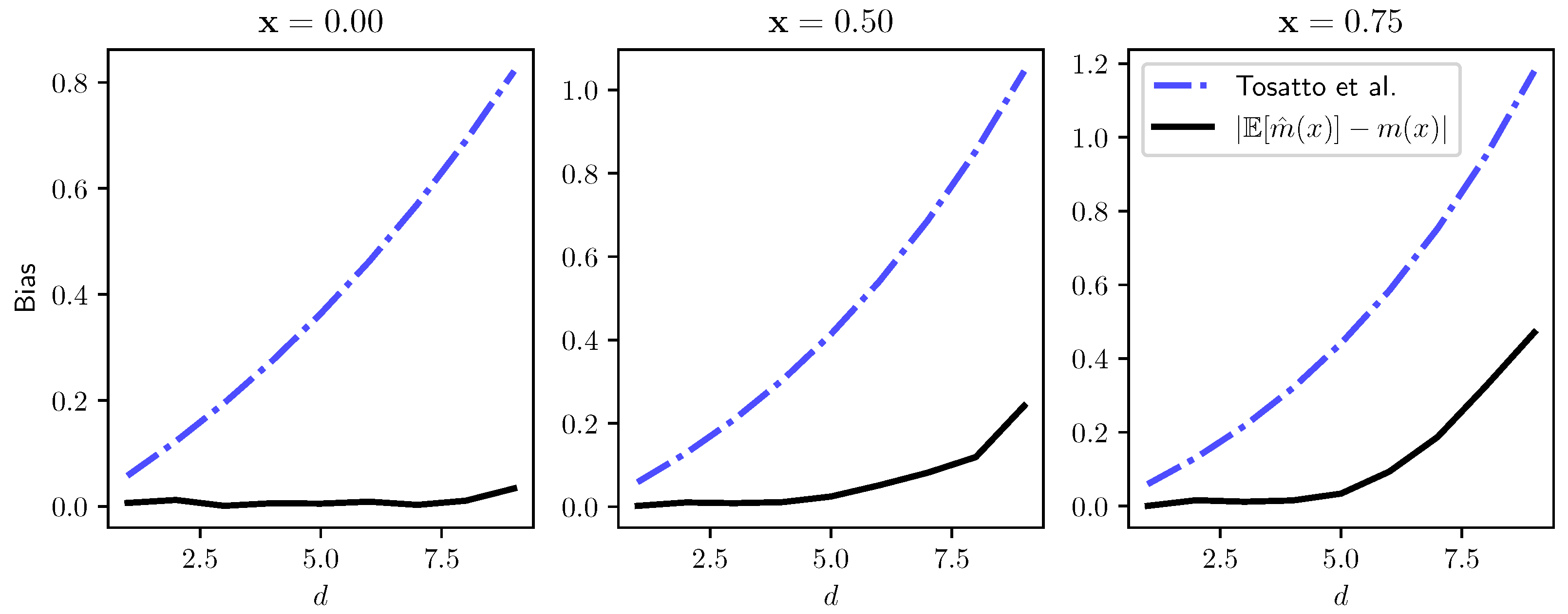
Multidimensional Analysis: We want to study if our bounds work in a multidimensional case and how much it overestimates the true bias (therefore, how tight it is). For this purpose, we took a linear function m ( x ) = 1 x where 1 is a column-vector of d ones. This function, for any dimension d, has a Lipschitz constant L m = 1 and is unbounded ( M = ) . We set a Gaussian design with zero mean and unit diagonal covariance. Since in higher dimensions, the estimation’s variance grows exponentially [22], we used a large number of samples ( n = 10 6 ), and we averaged over N = 10 5 independent estimations. In Figure 2 we show how the “true” bias (estimated numerically averaging over a thousand Nadaraya-Watson regressions) and our bound evolve with a growing number of dimensions d. Far from the low-density region x = 0 we notice that the bias tends to have a linear behavior, while close to the boundary the bias tends to be exponential. We can observe that our bound correctly bounds the bias in all the cases.
Realistic Scenario: Let us consider the regression problem of the dynamics of an under-actuated pendulum of length l and mass m. In particular, the state of the pendulum can be described by its angle α and its angular rotation α ˙ . Furthermore, a force u can be applied to the pendulum. The full system is described by,
α ¨ = 3 m l 2 u 3 g 2 l sin ( α + π ) ,
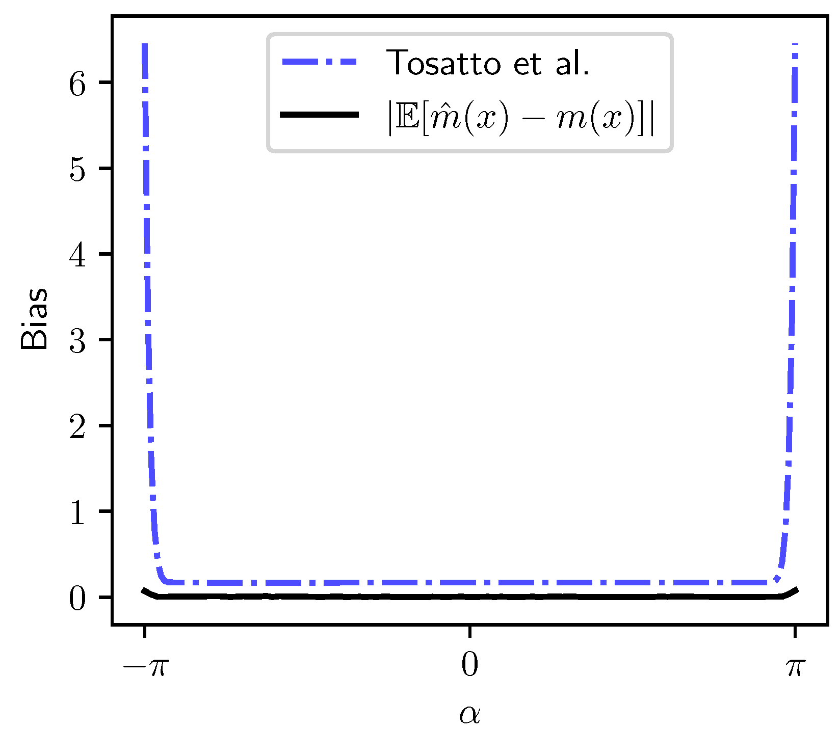
where g is the gravitational acceleration. In practice, when this model is discretized in time, the next state is estimated via numerical integration. Fort this reason, the Lipschitz constant L m is unknown. Notice that also m and m required by the Rosenblatt’s analysis are unknown. We estimated the Lipschitz constant L m by selecting the highest ratio | y i y j | / | x i x i | in the dataset. In our analysis, we want to predict all the states with fixed α ˙ = 0 , u = 0 , but variable α [ π , π ] . In order to generate the dataset, we use the simulator provided by gym [27]. To train our models, we generate tuples of α , α ˙ , u by sampling independently each variable from a uniform distribution i.e., α Uniform ( π , π ) , α ˙ Uniform ( 8 , 8 ) and u Uniform ( 2 , 2 ) (hence, L f = 0 ). We fit 100 different models with 50,000 samples. We choose a Gaussian kernel with bandwidth h = [ 0.2 , 0.2 , 0.2 ] . Figure 3 depicts our bound and the estimated bias. We notice the bias is low and increases close to the boundaries. Our upper bound is tight, but, as expected, it becomes overly pessimistic in the boundary region.
6. Applications

Our bound can be applied alongside any use of the Nadaraya-Watson regression estimate. In this section, we want to point out an interesting application in reinforcement learning. In reinforcement learning, we aim to approximate, from samples, an optimal behavior of an agent acting in a given environment. To do so, one can find a so-called “value-function” that determines how well the agent behaves. This function can be approximated using dynamic programming combined with functional approximators such as neural networks [28], but using also regression-trees [29], Gaussian processes [4], etc. In our prior work [30], we used the presented bound to subsequently bound the bias of the value function estimated via Nadaraya-Watson regression.

7. Conclusions

The Nadaraya-Watson kernel regression is one of the most well-known nonparametric estimator, used in a wide range of applications. Its asymptotic bias and variance are well-known in the literature. However, to the best of our knowledge, such an estimator’s bias has never been bounded before. In this paper, we proposed a hard bound of the bias that requires mild assumptions. Our proposed bound is numerically tight and accurate for a large class of regression functions, kernels, and random designs. We believe that providing hard, non-probabilistic guarantees on a regression error is an essential step in adopting data-driven algorithms in real-world applications. Our future research will focus on extending the bias analysis to a broader class of kernel functions and with a finite-samples analysis.

Author Contributions

S.T. conceived of the presented idea, developed the theory and performed the numerical simulations. R.A. verified the analytical method. Both S.T. and R.A. wrote the paper. All authors provided critical feedback and helped shape the research, analysis and manuscript. All authors have read and agreed to the published version of the manuscript.

Funding

This research received no external funding.

Acknowledgments

Authors are grateful to three anonymous referees and the editor for their valuable comments and suggestions, which certainly improved the presentation and quality of the paper.

Conflicts of Interest

The authors declare no conflict of interest.

Appendix A. Theorems Derivation

In order to provide proofs of the stated Theorems, we need to introduce some quantities and to state some facts that will be used in our proofs.
Proposition A1.
With a R , h 0 and c R ,
0 a k i x h e x L f d x = B i ( a / h , c h ) .
Proposition A2.
With a , b 0 , h i > 0 and L f 0 ,
a b k i x h i e | x | L f d x = h i B i ( b / h i , L f h i ) h i B i ( a / h , L f h i ) = ψ i ( a , b ) .
Proposition A3.
With a , b 0 , h i > 0 and L f 0 ,
a b k i x h i e | x | L f d x = h i B i ( b / h i , L f h i L f ) h i B i ( a / h i , L f h i ) = ζ i ( a , b ) .
Proposition A4.
With a R , h 0 and c R ,
0 a k i x h e x c x d x = h i 2 C i ( a / h , c h ) .
Proposition A5.
With a , b 0 , h i > 0 and L f 0 ,
a b k x h i e | x | L f | x | d x = h i 2 C i ( b / h , L f h i ) + C i ( a / h i , L f h i ) = ξ i ( a , b ) .
Definition A1.
Integral on a d-interval
Let C Ω ( τ , τ + ) with τ , τ + R ¯ d . Let the integral of a function f : C R defined on C be defined as
C f ( x ) d x = τ 1 τ 1 + τ 2 τ 2 + τ d τ d + f ( [ x 1 , x 2 , , x d ] ) d x d d x 2 d x 1 .
Proposition A6.
There is a function g : Y R such that
f X ( x ) = e g ( x ) Y e g ( x ) d x
and, given A2, | g ( x ) g ( y ) | L f | x y | y D .
Proposition A7.
Independent Factorization
Let C Ω ( τ , τ + ) where τ , τ + R d , and f i : R R ,
C i = 1 d f i ( x i ) d x = i = 1 d C f i ( x i ) d x .
Proposition A8.
Given C Ω ( τ , τ + ) , p : R R , q : R R ,
C i = 1 d p ( z i ) k = 1 d g ( z k ) d z = k = 1 d i k d τ i τ i + p ( z ) d z τ k τ k + p ( z ) q ( z ) d z .
Proof. 
Proof of Theorem 2:
| E lim n f ^ n ( x ) m ( x ) | = | E lim n i = 1 n K h ( x x i ) y i j = 1 n K h ( x x j ) m ( x ) | = | E lim n n 1 i = 1 n K h ( x x i ) y i n 1 j = 1 n K h ( x x j ) m ( x ) | = | E Y K h ( x z ) m ( z ) ε ( z ) f X ( z ) d z Y K h ( x z ) f X ( z ) d z m ( x ) | = | Y K h ( x z ) m ( z ) f X ( z ) d z Y K h ( x z ) f X ( z ) d z m ( x ) | = | Y K h ( x z ) m ( z ) m ( x ) f X ( z ) d z Y K h ( x z ) f X ( z ) d z | = | Y K h ( x z ) m ( z ) m ( x ) f X ( z ) d z | | Y K h ( x z ) f X ( z ) d z | .
We want to obtain an upper bound of the bias. Therefore we want to find an upper bound of the numerator and a lower bound of the denominator.
Lower bound of the Denominator:
The denominator is always positive, so the module can be removed,
Y K h ( x z ) f X ( z ) d z = Y f X ( z ) i = 1 d k z i h i d z D f X ( z ) i = 1 d k z i h i d z ( since D Y and the integrand is always non-negative ) = e g ( x ) Y e g ( z ) d z D e g ( z ) g ( x ) i = 1 d k z i h i d z ( Prop . A 6 ) = f X ( x ) D ¯ e g ( x + l ) g ( x ) i = 1 d k l i h i d l let l = z x and D ¯ Ω ( δ , + δ + ) f X ( x ) D ¯ e | l | L f i = 1 d k l i h i d l ( Axiom A 2 + Lipschitz Inequality ) = f X ( x ) D ¯ i = 1 d e | l i | L f k l i h i d l
Now considering Propositions A1 and A7, we obtain
+ K h ( x z ) f X ( z ) d z f X ( x ) i = 1 d ψ i ( δ i , δ i + ) .
Upper bound of the Numerator:
| Y K h ( x z ) m ( z ) m ( x ) f X ( z ) d z | Y K h ( x z ) m ( z ) m ( x ) f X ( z ) d z = G K h ( x z ) m ( z ) m ( x ) f X ( z ) d z + Y \ G K h ( x z ) m ( z ) m ( x ) f X ( z ) d z G K h ( x z ) m ( z ) m ( x ) f X ( z ) d z + f X ( x ) M Y \ G K h ( x z ) d z = e g ( x ) Y e g ( z ) d z G e g ( z ) g ( x ) K h ( x z ) m ( z ) m ( x ) d z + f X ( x ) M Y \ G K h ( x z ) d z f X ( x ) G e g ( z ) g ( x ) K h ( x z ) m ( z ) m ( x ) d z + M D
where
D = Y \ G K h ( x z ) d = lim ω + i = 1 d x i ω x i + ω k i x i z h i d z i = 1 d x i γ i x i + γ i + k i x i z h i d z = lim ω + i = 1 d h i Φ i ω h i i = 1 d h i Φ i γ i + h + h i Φ i γ i h i .
Let F Ω ( x ϕ , x + ϕ + ) G , we will later define at our convenience.
f X ( x ) G e g ( z ) g ( x ) K h ( x z ) m ( z ) m ( x ) d z + M D = f X ( x ) ( F e g ( z ) g ( x ) K h ( x z ) m ( z ) m ( x ) d z + G \ F e g ( z ) g ( x ) K h ( x z ) m ( z ) m ( x ) d z + M D ) f X ( x ) ( F e g ( z ) g ( x ) K h ( x z ) m ( z ) m ( x ) d z + M G \ F e g ( z ) g ( x ) K h ( x z ) d z + M D ) = f X ( x ) ( F ¯ e g ( x + l ) g ( x ) K h ( l ) m ( x + l ) m ( l ) d l + M G ¯ \ F ¯ e g ( x + l ) g ( x ) K h ( l ) d l + M D ) with l = z x , F ¯ Ω ( ϕ , ϕ + ) and G ¯ Ω ( γ , γ + ) f X ( x ) F ¯ e L f | l | K h ( l ) L m l d l + M G ¯ \ F ¯ e L f | l | K h ( l ) d l + M D ( A 2 , A 3 + Lipschitz Inequality )
The first integral instead can be solved with Propositions A3, A5 and A8,
F ¯ e L f | l | K h ( l ) L m l d l = F ¯ i = 1 d k l h i e | l | L f L m i = 1 d | l i | d l d l = L m k = 1 d i k d ϕ i ϕ i + k l h i e | l | L f d z ϕ k ϕ k + k l h e | l | L f | l i | d l ( Prop . A 8 ) = L m k = 1 d ξ k ( ϕ k , ϕ k + ) i k d ζ i ( ϕ i , ϕ i + ) .
The second integral can be solved using Propositions A1 and A7,
G \ F e L f | l | K h ( l ) d z = G e L f | l | K h ( l ) d l F e L f | l | K h ( l ) d l = i = 1 d ζ i ( γ i , γ i + ) i = 1 d ζ i ( ϕ i , ϕ i + ) .
A good choice for F is ϕ i = min ( γ i , M / L f ) and ϕ i + = min ( γ i + , M / L f ) , as in this way we obtain a tighter bound. In last analysis,
| E lim n m ^ n ( x ) m ( x ) | L m k = 1 d ξ k ( ϕ i k , ϕ i k ) i k d ζ ( ϕ i , ϕ i + ) + M i = 1 d ζ ( γ i , γ i + ) i = 1 d ζ ( ϕ i , ϕ i + ) + D i = 1 d ψ i ( δ i , δ i + )
showing the correctness of Theorem 2. □
In order to prove Theorem 3 we shall note that Y G F , therefore the lower bound can be bounded by
Y K h ( x z ) f X ( z ) d z = Y f X ( z ) i = 1 d k i x i z i h i d z f X ( x ) Y ¯ i = 1 d k i l i h i e l i L f d l = f X ( x ) i = 1 d ψ i ( υ i , υ i + )
for the numerator, instead
| Y K h ( x z ) m ( z ) m ( x ) f X ( z ) d z | f X ( x ) Y e g ( z ) g ( x ) K h ( x z ) m ( z ) m ( x ) d z f X ( x ) Y ¯ e L f | l | K h ( l ) L m l d l where Y ¯ Ω ( υ , υ + )
and therefore, for the reasoning already made for Theorem 2,
| E lim n m ^ n ( x ) m ( x ) | L m k = 1 d ξ k ( υ k , υ k + ) i k d ζ i ( υ i , υ i + ) i = 1 d ψ i ( υ i , υ i + )
where ξ A k , ζ , Ψ , φ are defined as in Theorem 2 and ϕ i = υ i , ϕ i + = υ i + .

Appendix B. Kernels

Appendix B.1. Gaussian Kernel

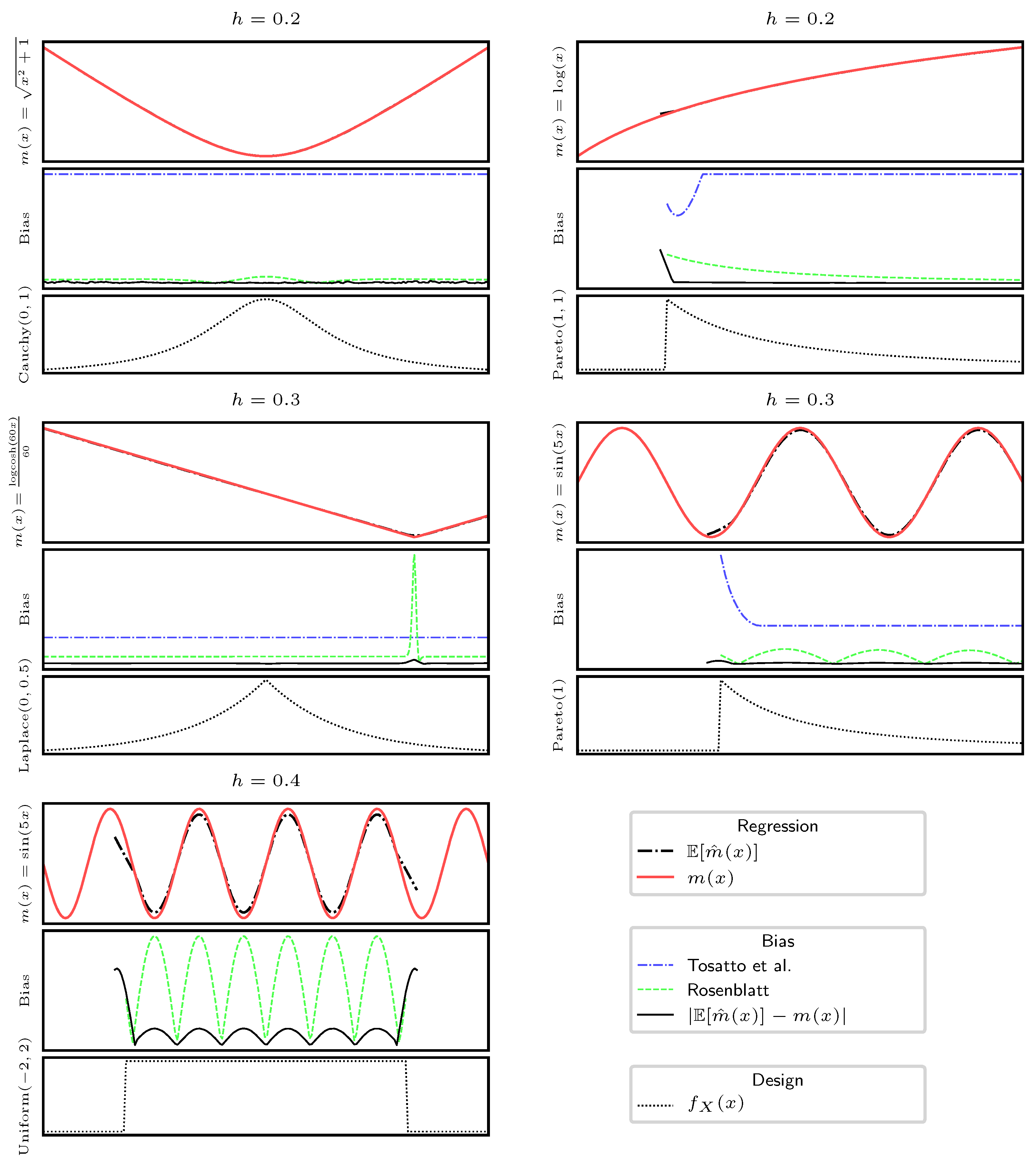
Figure A1. Same experiment as in Figure 1, with Gaussian Kernels.
Stats 04 00001 g0a1

Appendix B.2. Box Kernel

The box kernel, defined as k ( x ) = I ( x ) , has B ( a , c ) = g B ( a , c ) g B ( 0 , c ) and C ( a , c ) = g C ( a , c ) g C ( 0 , c ) , where
g B ( x , c ) = k ( x ) e x c d x = 0 if x < 1 e c e 2 c 1 c if x > 1 , e c e c x + c 1 c otherwise ( + const ) , g C ( x , c ) = k ( x ) e x c x d x = 0 if x < 1 e c c e 2 c e 2 c + c + 1 c 2 if x > 1 , e c c x e c x + c e c x + c + c + 1 c 2 otherwise ( + const ) ,
We show the results of a numerical simulation using the Box kernel in Figure A2.
Figure A2. Same experiment as in Figure 1, with Box Kernel.
Stats 04 00001 g0a2

Appendix B.3. Triangular Kernel

The triangular kernel, defined as k ( x ) = I ( x ) ( 1 | x | ) , has B ( a , c ) = g B ( a , c ) g B ( 0 , c ) and C ( a , c ) = g C ( a , c ) g C ( 0 , c ) , where
g B ( x , c ) = k ( x ) e x c d x = 0 if x < 1 e c x ( e c x + c c ( x + 1 ) 1 ) c 2 if 1 x 0 , e c x ( c ( x 1 ) 2 e c x + e c x + c + 1 ) c 2 if 0 < x 1 , e c e c 1 2 c 2 if x > 1 , ( + const ) , g C ( x , c ) = k ( x ) e x c x d x = 0 if x < 1 e c x ( c 2 x ( x + 1 ) c ( e c x + c + 2 x + 1 ) + 2 ( e c x + c 1 ) ) c 3 if 1 x 0 , e c x ( c 2 ( x 1 ) x c ( e c x + c 2 x + 1 ) + 2 ( e c x c + 1 2 e c x ) ) c 3 if 0 < x 1 , e c ( e c 1 ) ( e c ) c + c 2 e c + 2 c 3 if x > 1 , ( + const ) ,
We show the results of a numerical simulation using the Triangular kernel in Figure A3.
Figure A3. Same experiment as in Figure 1, with Triangular Kernel. Note that this particular kernel, does not have finite bound for L f = 0 .
Stats 04 00001 g0a3

References

  1. Bansal, R.; Gallant, A.R.; Hussey, R.; Tauchen, G. Nonparametric Estimation of Structural Models for High-Frequency Currency Market Data. J. Econom. 1995, 66, 251–287. [Google Scholar] [CrossRef] [Green Version]
  2. Nguyen-Tuong, D.; Peters, J. Using Model Knowledge for Learning Inverse Dynamics. In Proceedings of the International Conference on Robotics and Automation, Anchorage, AK, USA, 3–7 May 2010; pp. 2677–2682. [Google Scholar]
  3. Wang, J.; Hertzmann, A.; Fleet, D.J. Gaussian Process Dynamical Models. Adv. Neural Inf. Process. Syst. 2006, 27, 1441–1448. [Google Scholar]
  4. Deisenroth, M.P.; Rasmussen, C.E. PILCO: A Model-based and Data-efficient Approach to Policy Search. In Proceedings of the 28th International Conference on International Conference on Machine Learning, ICML’11, Omnipress, Bellevue, WA, USA, 28 June–2 July 2011; pp. 465–472. [Google Scholar]
  5. Kroemer, O.; Ugur, E.; Oztop, E.; Peters, J. A Kernel-Based Approach to Direct Action Perception. In Proceedings of the International Conference on Robotics and Automation, Saint Paul, MN, USA, 14–18 May 2012; pp. 2605–2610. [Google Scholar]
  6. Kroemer, O.B.; Peters, J.R. A Non-Parametric Approach to Dynamic Programming. In Advances in Neural Information Processing Systems; Curran Associates, Inc.: Dutchess County, NY, USA, 2011; pp. 1719–1727. [Google Scholar]
  7. Ormoneit, D.; Sen, S. Kernel-Based Reinforcement Learning. Mach. Learn. 2002, 49, 161–178. [Google Scholar] [CrossRef] [Green Version]
  8. Moosavi-Dezfooli, S.M.; Fawzi, A.; Frossard, P. Deepfool: A Simple and Accurate Method to Fool Deep Neural Networks. In Proceedings of the IEEE Conference on Computer Vision and Pattern Recognition, Las Vegas, NV, USA, 26 June–1 July 2016; pp. 2574–2582. [Google Scholar]
  9. Backurs, A.; Indyk, P.; Wagner, T. Space and Time Efficient Kernel Density Estimation in High Dimensions. Adv. Neural Inf. Process. Syst. 2019, 32, 15799–15808. [Google Scholar]
  10. Charikar, M.; Siminelakis, P. Hashing-Based-Estimators for Kernel Density in High Dimensions. In Proceedings of the 58th Annual Symposium on Foundations of Computer Science (FOCS), Berkeley, CA, USA, 15–17 October 2017; pp. 1032–1043. [Google Scholar]
  11. Herrmann, E.; Gasser, T.; Kneip, A. Choice of Bandwidth for Kernel Regression when Residuals are Correlated. Biometrika 1992, I, 783–795. [Google Scholar] [CrossRef]
  12. Härdle, W.; Marron, J. Asymptotic Nonequivalence of Some Bandwidth Selectors in Nonparametric Regression. Biometrika 1985, 72, 481–484. [Google Scholar] [CrossRef]
  13. Köhler, M.; Schindler, A.; Sperlich, S. A Review and Comparison of Bandwidth Selection Methods for Kernel Regression. Int. Stat. Rev. 2014, 82, 243–274. [Google Scholar] [CrossRef] [Green Version]
  14. Ray, B.K.; Tsay, R.S. Bandwidth Selection for Kernel Regression with Long-Range Dependent Errors. Biometrika 1997, 84, 791–802. [Google Scholar] [CrossRef]
  15. Nadaraya, E.A. On Estimating Regression. Theory Probab. Its Appl. 1964, 9, 141–142. [Google Scholar] [CrossRef]
  16. Watson, G.S. Smooth Regression Analysis. Sankhyā Indian J. Stat. Ser. A 1964, 28, 359–372. [Google Scholar]
  17. Rosenblatt, M. Conditional Probability Density and Regression Estimators. Multivar. Anal. II 1969, 25, 31. [Google Scholar]
  18. Fan, J. Design-Adaptive Nonparametric Regression. J. Am. Stat. Assoc. 1992, 87, 998–1004. [Google Scholar] [CrossRef]
  19. Fan, J.; Gijbels, I. Variable Bandwidth and Local Linear Regression Smoothers. Annals Stat. 1992, 20, 2008–2036. [Google Scholar] [CrossRef]
  20. Mack, Y.; Müller, H.G. Convolution Type Estimators for Nonparametric Regression. Stat. Probab. Lett. 1988, 7, 229–239. [Google Scholar] [CrossRef]
  21. Wasserman, L. All of Nonparametric Statistics; Springer: New York, NY, USA, 2006. [Google Scholar]
  22. Györfi, L.; Kohler, M.; Krzyzak, A.; Walk, H. A Distribution-Free Theory of Nonparametric Regression; Springer Science & Business Media: Berlin/Heidelberg, Germany, 2006. [Google Scholar]
  23. Miculescu, R. A Sufficient Condition for a Function to Satisfy a Weak Lipschitz Condition. Math. Rep. 2007, 9, 275–278. Available online: http://www.imar.ro/journals/Mathematical_Reports/Pdfs/2007/3/miculescu.pdf (accessed on 29 December 2020).
  24. Parzen, E. On Estimation of a Probability Density Function and Mode. Ann. Math. Stat. 1962, 33, 1065–1076. [Google Scholar] [CrossRef]
  25. Rosenblatt, M. Remarks on Some Nonparametric Estimates of a Density Function. Ann. Math. Stat. 1956, 832–837. [Google Scholar] [CrossRef]
  26. Wood, G.R.; Zhang, B.P. Estimation of the Lipschitz Constant of a Function. J. Glob. Opt. 1996, 8, 91–103. [Google Scholar] [CrossRef]
  27. Brockman, G.; Cheung, V.; Pettersson, L.; Schneider, J.; Schulman, J.; Tang, J.; Zaremba, W. OpenAI Gym. arXiv 2016, arXiv:1606.01540. [Google Scholar]
  28. Mnih, V.; Kavukcuoglu, K.; Silver, D.; Rusu, A.A.; Veness, J.; Bellemare, M.G.; Graves, A.; Riedmiller, M.; Fidjeland, A.K.; Ostrovski, G.; et al. Human-Level Control Through Deep Reinforcement Learning. Nature 2020, 518, 529–533. [Google Scholar] [CrossRef]
  29. Ernst, D.; Geurts, P.; Wehenkel, L. Tree-Based Batch Mode Reinforcement Learning. J. Mach. Learn. Res. 2005, 6, 503–556. [Google Scholar]
  30. Tosatto, S.; Carvalho, J.; Abdulsamad, H.; Peters, J. A Nonparametric Off-Policy Policy Gradient. In Proceedings of the International Conference on Artificial Intelligence and Statistics, Virtual Conference, 26–28 August 2020. [Google Scholar]
Figure 1. We propose some simulations of Nadaraya-Watson regression with different designs, regression functions, and bandwidths. (a)–(c) use Gaussian kernels, while (d) and (e) use Triangle and Box kernels, respectively. The regression function m ( x ) is represented with a solid line, while the Nadaraya-Watson estimate m ^ ( x ) is represented with a dash-dotted line in the top subplot of each experiment. In the second subplots, it is possible to observe the true bias (solid line), as well as our upper bound (dashed line) and Rosenblatt’s estimate (dash-dotted line). The bottom subplots depict the design used. The bandwidth used for the estimation is denoted with h. It is possible to observe that Rosenblatt’s estimate often under or overestimates the bias, e.g., subfigures (b) and (c). In all the different test conditions, our method correctly upper bounds the bias.
Stats 04 00001 g001
Figure 2. We propose a study on how the bias varies w.r.t. the dimension. While the bias grows almost linearly in the high density region (i.e., x = 0 ), it tends to grow exponentially in lower densities (i.e., x = 0.75 ). In both cases, our bound perform correctly.
Stats 04 00001 g002
Figure 3. Experiment on the under-actuated pendulum. Our bound gives the possibility to ensure that E [ m ( x ) m ^ ( x ) ] does not exceed a certain quantity. In this example, it is possible to observe that the bias is correctly bounded.
Stats 04 00001 g003
Table 1. Examples of parameters to use for different univariate random design.
DistributionDensity Y D L f
Laplace ( μ , λ ) 1 2 λ exp | x μ | λ ( , + ) ( , + ) λ 1
Cauchy ( μ ; γ ) π γ + π ( x μ ) 2 γ 1 ( , + ) ( , + ) 2 ( z μ ) γ 2 + ( z μ ) 2 1
Uniform ( a , b ) 1 b a if a x b 0 otherwise ( a , b ) ( a , b ) 0
Pareto ( α ) α x α + 1 if x 1 0 otherwise ( 1 , + ) ( 1 , + ) 1 + α
Normal ( μ , σ ) 1 2 π σ 2 exp ( x μ ) 2 2 σ 2 ( , + ) ( a , b ) f μ , σ ( a , b )
Publisher’s Note: MDPI stays neutral with regard to jurisdictional claims in published maps and institutional affiliations.