


Highlights
What are the main findings?
- In this paper, we describe the development of an open-source Python-based generalizable model for electrodialysis-based ocean alkalinity enhancement (OAE) plants.
- The model is used to (1) evaluate the performance of a theoretical case study OAE plant with different locally available energy sources and (2) explore which microgrid and scale can enable the plant to become profitable without carbon credits by selling co-products such as dilute acid or recycled concrete aggregate.
- The results show that the example OAE plant could be profitable without carbon credits at commercial scales, which indicates that similar commercial-scale plants could either require low-cost carbon credits to break even or be profitable without them if they use low-cost electricity and sell their co-products.
- Additional work is required to verify the results as more data on these plants become publicly available; however, this model can still act as a helpful preliminary tool for evaluating potential OAE plant deployments.
Abstract
Electrochemical ocean alkalinity enhancement is a form of marine carbon dioxide removal, a rapidly growing industry that is powered by efficient onshore or offshore energy sources. As more and larger deployments are being planned, it is important to consider how variable energy sources like tidal energy can impact plant performance and costs. An open-source Python-based generalizable model for electrodialysis-based ocean alkalinity enhancement has been developed that can capture key system-level insights of the electrochemistry, ocean chemistry, acid disposal, and co-product creation of these plants under various conditions. The model additionally accounts for hybrid energy system performance profiles and costs via the National Laboratory of the Rockies’ H2Integrate tool. The model was used to analyze an example theoretical plant deployment in North Admiralty Inlet, including how the plant is impacted by the available energy sources in the region and the scale at which plant costs are covered by the co-products it generates, such as recycled concrete aggregates, without requiring carbon credits. The results show that the example plant could be profitable without carbon credits at commercial scales of 100,000 to 1 million tons of carbon dioxide removal per year, so long as it uses low-cost electricity sources and either sells acid or recovers recycled concrete aggregates with about 1 molar acid concentrations, though more research is needed to confirm these results.
1. Introduction
Electrochemical ocean alkalinity enhancement (OAE) is a type of marine carbon dioxide removal (mCDR), a growing industry that uses the ocean to capture, store, and/or utilize carbon dioxide (CO2) [1,2]. OAE and other electrochemical mCDR deployments are currently at a developmental level of 100 to 10,000 tons of yearly CO2 removal (tCO2/yr) [3,4,5]. Developers aim to build commercial-scale plants that will remove 100,000 to 1 million tCO2/yr [5,6]. To maximize their mCDR scales, these plants will require substantial efficient energy sources onshore or offshore; there are potentially enough marine and other efficient offshore energy sources available in U.S. waters to enable the industry to reach gigaton-per-year scales of mCDR [2]. Figure 1 shows an example of an OAE plant powered by efficient offshore energy sources.
Figure 1.
Graphic illustration of an example ocean alkalinity enhancement (OAE) plant powered with efficient energy sources (A). The plant pumps in seawater (B), increases the water’s alkalinity, and then releases the effluent back into the ocean (C). In this case the plant is powered with wind (D), solar (E), tidal (F), and wave energy (G). Meanwhile, a wave-energy-powered monitoring system evaluates the biogeochemical impacts of the plant on the surrounding region (H).
Electrochemical OAE produces acid and base—hydrochloric acid (HCl) and sodium hydroxide (NaOH)—from pumped seawater using electrochemical technologies such as electrodialysis (ED) [1,2,7,8]. The base is added to surrounding waters to enable mCDR. This increases local alkalinity and converts a portion of the dissolved CO2 into bicarbonate ions, which prevents the gas from re-entering the atmosphere, potentially for thousands of years [1,2,7,8]. The reduction of acidity and dissolved CO2 concentration drives more atmospheric CO2 into surface waters [1,2,7,8]. Meanwhile, the generated acid from the plant is sold or neutralized above or below ground [1,2,7,8] (Figure 2).
Figure 2.
Illustration of the simplified electrochemical OAE process. Acid and base are made from seawater. The base is added to the surrounding ocean to enable CO2 removal while the acid is sold or neutralized elsewhere [2].
Historically, the generated acid from electrochemical OAE plants has been considered to be too dilute for industrial application, and further concentrating it to improve its marketability has thus far proven to be uneconomical [9]. However, recent analysis from Jin et al. has shown that the dilute salty acid generated by these plants could be used to recover recycled concrete aggregate (RCA) from waste concrete [10]. RCA can be used in new construction, especially since natural aggregates used in concrete production are becoming more scarce due to global demand and overmining [10]. Jin et al. identified that by placing mortar-covered RCA from waste concrete in solutions of dilute HCl (with salt and acid concentrations similar to those anticipated from electrochemical OAE plants) and by mixing the slurry in a rotary drum, the RCA can neutralize the acid, and the acid can also improve the strength, durability, and value of the RCA enabling it to be used in highly demanding construction projects like building roads or bridges [10]. Note that mortar exposed to air for long periods of time can develop calcium carbonate (CaCO3) deposits, which would release CO2 when reacted with acid [10]. As a result our work focuses on using recently detonated or uncarbonated waste concrete. The upcycled waste concrete can be sold for $10–$40/ton and can potentially be a large-scale market for the dilute acid generated by electrochemical OAE plants [10].
As electrochemical OAE deployments increase in number and scale, it is critical to develop modeling tools to evaluate how their performance and costs can be impacted by the efficient energy sources they utilize, as these energy profiles can be quite temporally variable. One of the benefits of ED-based electrochemical mCDR systems is that they can directly use variable power. By contrast, electrolysis-based systems require more consistent power profiles [11]. Additionally, since the energy needs for the ED system are typically much greater than that of the seawater, acid, and base pumping system (which have median energy needs of 1540 kWh/tCO2 and 567 kWh/tCO2, respectively), these mCDR systems can utilize chemical storage tanks to continue operation when power availability is low to increase overall yearly rates of OAE [2,11].
The goal of this project was to develop a generalizable open-source electrochemical OAE plant model that can model plant operation and cost with variable hybrid energy sources and with different options of acid disposal. As has been done with the team’s previous work on a similar electrochemical direct ocean capture model, the newly developed Python-based model has been integrated into the National Laboratory of the Rockies’ (NLR’s) hybrid energy software H2Integrate (H2I) to enable simulating a plant powered with marine and other efficient energy sources given the energy resources available at a potential deployment location [11,12]. The acid produced by the plant can be sold to a facility for RCA recovery, or the recovery can be conducted on-site. With these options, plant configurations and scales can be explored in which enough co-products can be sold to minimize the cost of carbon credits required for the plant to break even (i.e., recover the cost of its investment with no additional profit) or in which the plant could avoid needing carbon credits to be profitable.
2. Materials and Methods
The overall OAE plant model is visualized in Figure 3 and accounts for (1) pumping large volumes of seawater or brine, (2) using a fraction of the pumped fluid to electrochemically produce acidic and basic solutions via the ED system, (3) adding the base solution to the neutral seawater or brine, (4) disposing of the acid either by selling it or its co-products, and (5) storing some of the base (and acid depending on the acid disposal option) in storage tanks for later use. The time step of the model is set to 1 h. The model was made using Python 3.10.
Figure 3.
Diagram describing the full modeled OAE system, which is a simplification of OAE plants described in literature and deployed in industry [3,9,13]. The colors of the tubes indicate the different types of solutions moving through the system: blue is seawater, red is acid, light blue is base, and dark blue is alkaline seawater.
The input energy and the volume of base available in the chemical storage tank determine the hourly output of the Python-based model. These inputs dictate the operational scenario to use (for instance, whether conducting OAE or filling the tanks needs to be prioritized). Together the hourly inputs and operational scenario determine the hourly outputs of the plant (e.g., the pH and flow rate of the effluent alkalized seawater and the generated acid). The outputs vary with the available input energy due to the ED system’s ability to operate flexibly with variable power, which has been shown for ED-based desalination [14,15,16].
The ED system’s ability to operate with variable power is approximated by splitting the ED system into discrete “units”. Each of these units have the same constant power and flow rate needs and the total number of ED units approximates the electrochemical system’s ability to operate with direct power inputs (see Figure 4) [11].
Figure 4.
Diagram describing the electrodialysis (ED) system of the OAE model.
These discrete units enable the plant to operate flexibly by switching on and off depending on the amount of power available [11]. For instance, if there is only enough power available for half of the total units, then half as much seawater will be pumped to create half as much acid and base, which will either be stored in the tanks or used for OAE. As a result, the number and power requirements of the individual ED units determine discrete ranges of output values. For computational efficiency, these ranges are determined for each operational scenario prior to the time-dependent analysis, and they are then referenced once the analysis begins.
The model utilizes four heuristic operational scenarios to consider how the generated base can be allocated for OAE [11]. In Scenario 1, the base is produced by the ED system and only used for OAE. In Scenario 2, some of the base is used for OAE while the rest is stored in a tank. In Scenario 3 there is not enough power to activate the ED system, but there is enough to use base from the tank for OAE. Scenario 4 considers the reverse: ED operation is possible but there is not enough power to pump seawater to dilute the base and release the alkaline seawater for OAE, so the generated base goes into storage (see Figure 5). These scenarios act as a structured approach to capture key system-level behaviors of ED-based OAE plants under variable power conditions [11].
Figure 5.
Operational scenarios for the OAE plant when the acid is sold.
The operational scenarios of the OAE plant can also vary depending on the acid disposal option selected. There are two options of acid disposal considered in this study: selling the acid or using it to recover RCA from recently detonated or uncarbonated waste concrete, which can be sold as a revenue stream. These options are described in more detail in Section 2.3. The RCA option involves neutralizing the acid with mortar-covered RCA, which contains calcium oxide (CaO), a strong base [10]. The neutralized seawater is then added to the alkaline effluent. Acid disposal occurs along with OAE, and therefore the acid is stored in its own tank (see Figure 6 for how using RCA for acid disposal impacts the operational scenarios). Future work can investigate alternate timing for acid disposal with RCA and incorporate models for other options of acid disposal, such as improving algae growth, enhanced mineralization, and mineral extraction [17,18,19].
Figure 6.
Operational scenarios for the OAE plant when recycled concrete aggregate (RCA) is recovered by the acid onsite.
The model was developed using details from literature about OAE and its acid disposal options along with advisement from an industry partner. As mentioned in Section 1, the OAE model is operated in conjunction with the H2I platform to examine plant performance and costs with realistic hybrid energy microgrids.
This section discusses the key components of the OAE model, including electrochemistry, ocean chemistry, acid disposal, pumping the chemical solutions and seawater, and costs (Section 2.1, Section 2.2, Section 2.3, Section 2.4, Section 2.5 and Section 2.6). It also describes the key modeling assumptions (Section 2.7) and the integration of the H2I hybrid energy model used to simulate the efficient energy sources (Section 2.8).
This study focuses on evaluating a theoretical developmental-level 10 ktCO2/yr scale electrochemical OAE plant, assumed to be connected to an existing theoretical desalination plant and therefore uses input brine rather than seawater. The parameters of the modeled example plant are shown in Table 1. Note that is the maximum amount of active ED units, and are the maximum power need and flow rate for the ED system, is the fraction of ED flow that becomes base, and are the concentrations of the generated acid and base, is the ratio of ED flow to intake flow, and are the pH and temperature of the intake brine/seawater, and are the concentrations of dissolved inorganic carbon (DIC) and salinity of the intake brine/seawater, and are the temperature increases from the ED and desalination systems, is the weight fraction of CaO in RCA, is the fraction of CaO that dissolves from the RCA, is the power need to mix the RCA and acid, is the fraction of RCA that can be sold, d is the days of the simulation, is the pump efficiency, the inputs refer to the pressure drop ranges of the active pumps, and is the hours of minimum OAE enabled by tank storage.
Table 1.
Parameters for the example 10 ktCO2/yr scale developmental-level OAE plant assumed to be connected to an existing theoretical desalination plant.
Most of the parameters used in this model were based on those used in literature [9,10,11,20,21]. Many of the OAE plant inputs were adapted from Ferella et al. [9] who assessed a roughly 1 ktCO2/yr scale system connected to a desalination plant. The and values from their work were scaled up by a factor of 10 for the analysis of the case study plant, while their values for , , , and were directly used and their pump inputs were estimated, see Section 2.9 for more details on the literature parameters used [9]. Their cost inputs were also scaled using a learning rate method, see Section 2.6. Meanwhile, the values for , , and were based on feedback from our industry partner.
The overall model was validated both by comparing the results for a 1 ktCO2/yr scale plant with inputs from Ferella et al. [9] and a 8 ktCO2/yr scale plant with inputs from our industry partner (see Section 2.9). Additionally, the operational scenarios were confirmed to function appropriately by examining the plant performance under an example sine wave power profile, which was also used to compare plant performance between selling acid and RCA (Section 2.10.1). The break-even carbon credit costs and performance of the developmental-level plant were then assessed under the two acid disposal options with microgrids containing different energy sources, as described in Section 2.10.2. The two microgrid configurations that resulted in the lowest break-even carbon credit costs were used to evaluate the plant at varying scales from developmental (1 to 10 ktCO2/yr) to commercial (100 to 1000 ktCO2/yr) to determine if revenue from the co-products could remove the need for carbon credits at commercial scales (Section 2.10.3) [3,4,5,6].
2.1. Electrochemistry Model
As described in Section 2, the ability of the ED system to use variable power is accounted for by splitting it into individual “units,” each with the same power, intake flow rate, output flow rates of acid and base, and concentrations of acid and base (Figure 4) [11]. In contrast to the previous work on the direct ocean capture model (which determined acid and base concentrations based on user ED efficiencies), the concentrations of acid and base are user inputs for the OAE model, as these values are more commonly reported and known by developers than ED efficiencies. However, the efficiencies of the ED system at producing acid and base ( and in Wh/mol HCl and Wh/mol NaOH, respectively) are still reported and determined using the equations below [11,22]:
where is the maximum power needed by the ED system in watts, and are the maximum output flow rates of the acid and base in m3/s, and are the concentrations of acid and base produced in mol/m3, is the input flow rate to the ED system in m3/s, and and are the concentrations of acid and base in the input seawater in mol/m3. and are direct inputs for the model while and are found by converting the input concentrations from mol/L to mol/m3. and are found using the pH of seawater, , which is typically around 8.1, and the water dissociation constant, , which is determined using the same equation as in our previous direct ocean capture work [11]:
Unlike the previous direct ocean capture model, the flow rates of acid and base are not assumed to be equal to each other; instead, a fraction of base flow () is used as a user input to determine the flow rates of acid and base [11]:
The power needs of the ED system (), the flow rates into the ED system (), and the output flow rates of acid and base ( and ) vary linearly with the number of active ED units, , but the concentrations of acid and base remain the same [11]. The minimum amount of active ED units, , is 1 as a default, and is the flow rate needed for one ED unit:
The overall intake of seawater for the OAE plant is determined by the number of active ED units since the ED flow rate is a fraction, , of the intake flow rate . By default the model assumes that 1% of the intake flow rate is used by the ED system, meaning that the intake flow rate is 100 times larger than the flow rate of the ED system, as was done in our prior direct ocean capture work and confirmed as reasonable by our OAE industry partner for this work [11]:
The input parameters for this model are shown in Table 1.
2.2. Ocean Chemistry Model
Unlike previous work, the seawater chemistry is not approximated as a carbonate buffer solution but instead utilizes PyCO2SYS (Version v2.0.0-b5), a Python toolbox that can account for additional chemical species in the marine carbonate system and calculate seawater characteristics such as pH and total alkalinity (TA) [11,23,24]. The ocean chemistry model relies on inputs for the initial DIC concentration, pH, ambient temperature, and salinity. Additionally, this part of the model accounts for the slight temperature increases that the ED system can have on the seawater, , which is 2 °C by default per feedback from our industry partner.
In this case, our team was interested in modeling how the system could be co-located with a desalination plant to utilize the effluent brine of the plant in place of seawater, which could minimize costs [9,25]. Therefore, the salinity input, , and DIC input, , were higher than usual for seawater (Table 1). Additionally, the desalination process can increase the temperature of the brine, , which by default is also assumed to be roughly 2 °C. This model is generalizable, so if a user prefers to use saltwater inputs, the temperature increase can be set to zero (Table 1). Inputs to PyCO2SYS included pH, salinity, temperature, and concentrations of TA, DIC, and calcium, while other parameters were left at their default values [23,24]. Additionally the default methods for the equilibrium constant parameterization [26] and total pH scale [27] were used. See Section 2.7 for details on the assumptions made when using PyCO2SYS.
Base Addition
The resulting pH after the base addition in the third step of Figure 3 is determined by first finding the TA, salinity, and temperature of the mixed base and seawater solutions. The new values of TA and salinity in mol/m3 ( and ) were found by comparing the sum of moles divided by the change in volume or, in this case, the flow rate, as described in the following equations, where is the initial salinity converted from ppt to mol/m3:
The salinity in the base stream is lower than that of the brine/seawater stream since a portion of the salinity was consumed to create the higher concentration of base. Because of this, the model also alerts the user if the concentration of base or acid is higher than that of the salinity. Simply put: and . Additionally, since the brine/seawater is considered to have the same specific heat and density, the temperature of the mixed solutions, , can be found using the same formulation as that of the TA and salinity while accounting for the changes in temperature from the desalination system and the ED system:
After the TA, salinity, and temperature values of the mixed solution are determined they are used as inputs along with the DIC, which does not change since both solutions have the same DIC concentrations, into PyCO2SYS to determine the pH of the solution. Other inputs for PyCO2SYS are set to default conditions. The equations described in this section are specifically for the case where the acid is sold; see Section 2.3.1 for details on how the TA, salinity, and temperature are impacted by using RCA for acid disposal.
2.3. Acid Disposal Models
As described in Section 2, there are two methods of acid disposal that the model accounts for: selling the acid and using it to extract RCA from waste concrete. In this model it is assumed that the dilute acid can be sold directly to a separate facility that recovers RCA, or the model can account for recovering RCA on-site. Selling the acid directly only impacts the cost model described in Section 2.6, where the acid is valued at $9/ton [9]. The mass of the acid is determined by multiplying the average yearly acid volume produced by the density of seawater, which is about 1030 kg/m3. As shown in Figure 5, the acid production does not impact the OAE performed by the system if it is being sold. Recovering the RCA on-site (valued at $10–$40/ton) does impact the operation of the plant, as shown in Figure 6, by diluting the effluent with neutralized seawater and increasing the energy needs for the scenarios.
2.3.1. RCA Models
To determine the amount of RCA that can be produced by the plant, the model calculates how much RCA is needed to neutralize the acid to the pH of seawater, 8.1. Initially the RCA from the waste concrete contains a fraction of CaO, which when dissolved in seawater creates calcium hydroxide (Ca(OH)2) a strong base key to acid neutralization. Note that over time, some of the CaO in the waste concrete can react with CO2 to create solid CaCO3, which when reacted with acid can release CO2 back into the atmosphere [10]. To limit CO2 release and improve the efficiency of the neutralization, Jin et al. [10] recommended focusing on recently detonated or uncarbonated RCA, which this model does as well.
To dissolve the CaO into the acid and enable neutralization, Jin et al. [10] mixed RCA from waste concrete and dilute acid in a rotary drum. In this model, the concentration of CaO (or oxide, [O2−], also referred to as ) is determined by accounting for the initial mass of dry RCA added to the acid per unit volume ( in g/L or kg/m3), the weight fraction of CaO (, which was 8.5% in Jin et al. [10]), the fraction of CaO that dissolves into solution (, assumed to be about 95%), and the molar mass of CaO ():
Since each dissolved mole of CaO becomes one of Ca(OH)2, each mole of dissolved CaO becomes two moles of hydroxide (OH−). Therefore, the concentration of added alkalinity from the RCA () is such that: .
The TA after neutralization with the RCA () is therefore the sum of the acid’s TA () and the added alkalinity such that: . Note that is negative for the acid and the greater the acid concentration the lower the value and therefore the more needed. To determine an initial value for the loading of RCA needed for neutralization or , is calculated using PyCO2SYS for a target pH of 8.1, and the previously discussed equations in this section are rearranged such that:
This calculation is initially done by ignoring the effect of the dissolved calcium () from the CaO on the alkalinity and salinity and ignoring the impact of the exothermic reaction on the temperature of the solution. The added calcium, , is equivalent to that of the added oxide ([] = [] and ) and increases the salinity of the neutralized solution () such that:
The temperature change of the solution is dependent on the moles of CaO that react with the HCl in solution following the thermochemical equation:
where for every mole of CaO reacted, 186 kJ of heat are released, or kJ [28]. This heat is assumed to be absorbed by the neutralized seawater and the RCA. Additionally, assuming that both the rocks and the solution reach thermal equilibrium, then the final temperature of the neutralized seawater () can be found such that:
In the previous equations, refers to the density of the seawater (1030 kg/m3); is the initial temperature of the acid (); is the initial temperature of the RCA, which is equal to by default; is the specific heat of water, which is about 4.18 kJ/kgK; and is the average specific heat of common rocks, which is about 0.75 kJ/kgK [29]. Furthermore, represents the final mass of dry RCA loaded per unit volume of neutralized seawater (in g/L or kg/m3) that can be recovered from the process and sold, which is determined by first finding the dissolved mass of RCA per unit volume ( in g/L or kg/m3), where:
After first ignoring the impacts of the and the change in temperature, the model then iteratively solves for what value results in the target pH of 8.1 within 0.01 pH units while accounting for the proper salinity and calcium concentration and temperature in PyCO2SYS. This calculation starts with increasing the value of , found by ignoring the and temperature change by 0.01 g/L increments until 2 g/L is added. If no loading value is found that meets the pH tolerance, then the step size decreases to 0.001 g/L and the process is repeated. While evaluating this model, the pH of the loading found by ignoring the impacts of and temperature were consistently slightly lower than the target pH once the and temperature changes were accounted for, hence the tight range of values evaluated.
The mass of dry RCA from waste concrete ( in g) needed to neutralize the acid produced in each hourly time step is found by multiplying the volume of acid ( in L) by such that . Additional power is needed to move a large-scale rotary drum that can enable the neutralization and RCA recovery. Large-scale rotary drums or rock tumblers used in the concrete industry can use electric motors to rotate their contents and generally require about 1.543 W/g () based on their motor power rating and max weight capacity [20]. In this model it is assumed that the power scales linearly with the mass of the acid and RCA in the rotary drum. The mass of the slurry that can be processed is the sum of the mass of RCA and that of the acid (). The power needed for processing the RCA in each hourly time step ( in W) is therefore .
Jin et al. [10] found that about 3 h were needed for the RCA to neutralize the acid and become refined enough to be sold; however, our model assumes that as the technology and methodology improves and scales, this time requirement would become roughly hourly. This assumption was also made to simplify the RCA model so that it would have the same hourly time step as the rest of the OAE plant model.
As shown in Figure 6, the neutralized seawater produced in this process is mixed with the alkaline seawater used for OAE. The TA, salinity, temperature, and calcium concentration then change following the same method as that employed in Section 2.2 for finding the new TA, salinity, and temperature for the mixed seawater and base. PyCO2SYS is used to determine the new pH of the slightly diluted effluent:
The total amount of dry RCA that can be sold on average per year is determined by first finding the total mass of RCA used for neutralization over the course of a year ( in g/yr). This is found by summing the masses of RCA used to neutralize the acid for the number of days (d) of the simulation:
The ultimate weight of dry RCA that can be sold per year ( in g/yr) is less than what is used for neutralization since part of its mass ( in g/yr) dissolves into the seawater for neutralization:
The total amount of dry RCA that can be sold is also influenced by the fraction of the recovered RCA that is of high enough quality to be sold, . In this model is assumed to be close to 100%:
The final mass of dry RCA is valued at $10–$40/ton and incorporated into the cost model in Section 2.6. The inputs used in the RCA acid disposal model are described in Table 1.
2.4. Pumping Model
The pumps considered for the cases where acid is directly disposed of are displayed in Figure 7 and those for recovering RCA are shown in Figure 8. The pumps all use the same power equation shown below, where the power P of each pump depends on the efficiency , flow rate Q, and pressure drop :
Figure 7.
Diagram describing the pumps of the OAE model when acid is being sold. Note pump “ED4” is used in place of pump “O” in Scenario 4 (see Section 2.5 for more details) [11].
Figure 8.
Diagram describing the pumps of the OAE model when RCA is being sold. Note that no new pumps are used but their flow rates do vary.
As was done in our prior direct ocean capture model [11], the fluid flow in the pumps was assumed to be laminar and follow the Hagen-Poiseuille equation for fluid flow through a pipe. Since the dynamic viscosity of the fluid (), the pipe length (L), and the pipe radius (r) are assumed to be constant and not dependent on the pressure drop or fluid flow, the pressure drop is assumed to vary linearly with flow rate:
Such a relationship enables estimating the pressure drop for a flow rate given the minimum and maximum pressure drops and flow rate ranges:
Each pump has the same input efficiency but their ranges of flow rates and pressure drops vary, as shown in Table 1. The flow rates of each pump depend on the operational scenario and number of active ED units, see Section 2.5. For the example OAE plant, only pumps “O,” “ED,” “a,” “b,” and “ED4” have nonzero or non-atmospheric pressure drops, meaning the other pump power needs are assumed to be zero since the fluid flows by gravity. Note that the filtration unit is modeled as a pressure drop for pumps “O” and “ED4”.
2.5. Operational Scenarios
Including chemical storage tanks enables the model to apply a heuristic operational strategy to evaluate how the plant could operate under variable power availability, similar to what was done in our previous direct ocean capture plant model [11]. As described in Section 2, there are four primary operational scenarios. If RCA is used for acid disposal, then whenever OAE is done, so is the acid disposal, meaning that the acid is also stored in a separate tank when RCA is processed on-site. In Scenario 1 the tank is full, so the base generated by the ED system is used for OAE while the acid is disposed of. This can also be approximated to typical operation without considering chemical storage. In Scenario 2, there is enough energy to enable OAE but the tanks are not full; therefore, a portion of the chemical solutions generated during the time step is stored in the tanks while the rest is used for OAE. In Scenario 3, there is not enough power available to activate the ED system but there is enough to pump base from the tanks for OAE, and acid for disposal. Scenario 4 is triggered only when there is not enough base in the tanks for OAE to be done via Scenario 3, but there is just enough power to activate the ED system to fill the tanks. See Figure 5 and Figure 6 for what these operational scenarios look like for selling the acid and using it to recover RCA. Finally, Scenario 5 occurs when there is not enough power or volume to activate the other scenarios. If the modeled microgrid has a battery system then this power can be stored for later use, otherwise the power is excess.
The input and output ranges for each operational scenario (power needs, moles of NaOH added to the seawater, and effluent flow rate and chemistry) are initialized prior to simulating the plant’s performance at each time step. They are then referenced during the time-dependent analysis given the amount of power and tank volume available. These ranges are based on the number of active ED units, or equivalent for Scenario 3. The total number of cases within Scenarios 1, 3, and 4, , is therefore:
The example OAE plant has a maximum number of 10 ED units and by default has a minimum of 1 ED unit, meaning is 10 (Table 1). The specific hourly output values depend on the number of units or equivalent that can be activated at the hourly time step, . For scenarios 1, 3, and 4 all of the ED units are used to either solely conduct OAE and acid disposal or solely fill the tanks. However, in Scenario 2 there are more output values since the number of units conducting OAE, , versus filling the tanks, , can vary. In this scenario, filling the tank or tanks is prioritized while at least one ED unit is used for OAE and acid disposal. See our prior direct ocean capture model work for more details on how the output values from Scenario 2 are calculated and selected during the time-dependent analysis [11]. The overall power needs for each of these output cases depend on the number of ED units powered, flow rates into and out of the system, and the rotary drum if RCA is being recovered.
The default maximum volume of the base () and acid when RCA is being recovered (), depend on the total storage time () and the flow rates of base and acid provided by the minimum number of ED units:
These volumes were selected to enable the tanks to facilitate conducting the minimum OAE rate over the duration of the storage time, which is set to 12 h for the example plant [11].
To clarify the flow rates of acid and base sent to the tanks compared to those used for acid disposal and OAE they are labeled as , , , and , respectively. These flow rates are enabled by the acid and base pumps such that and , except for in Scenario 3 where the solutions are pumped from the tanks, are and . Note that is only nonzero if the RCA method is used for acid disposal. Additionally, and must be nonzero if any acid and base are flowing since pumps “a” and “b” enable these flow rates. The pumps and flow rates used for each of the four primary scenarios under direct acid disposal and using RCA are shown in Figure 9, Figure 10, Figure 11 and Figure 12 and Table 2, Table 3, Table 4, Table 5, Table 6, Table 7, Table 8 and Table 9.
Figure 9.
Diagram describing the seawater, acid, base, and effluent flows in Scenario 1 for when the acid is being sold and when the acid is used to recover RCA.
Figure 10.
Diagram describing the seawater, acid, base, and effluent flows in Scenario 2 for when the acid is being sold and when the acid is used to recover RCA.
Figure 11.
Diagram describing the seawater, acid, base, and effluent flows in Scenario 3 for when the acid is being sold and when the acid is used to recover RCA.
Figure 12.
Diagram describing the seawater, acid, base, and effluent flows in Scenario 4 for when the acid is being sold and when the acid is used to recover RCA.
Table 2.
Flow rates for Scenario 1 when the acid is sold.
Table 3.
Flow rates for Scenario 1 when RCA is recovered.
Table 4.
Flow rates for Scenario 2 when the acid is sold.
Table 5.
Flow rates for Scenario 2 when RCA is recovered.
Table 6.
Flow rates for Scenario 3 when the acid is sold.
Table 7.
Flow rates for Scenario 3 when RCA is recovered.
Table 8.
Flow rates for Scenario 4 when the acid is sold.
Table 9.
Flow rates for Scenario 4 when RCA is recovered.
2.6. Cost Model
The cost model adapts and modifies the methodology used by Ferella et al. [9] who conducted an in-depth cost analysis on a theoretical 1 ktCO2/yr developmental-level scale ED-based OAE plant connected to a desalination plant. The team also accounted for potential revenue from selling the dilute acid, which can be used to reduce the cost of carbon credits needed for the electrochemical OAE plant to break even or recover their investment () [9]. Though the analysis by Ferella et al. [9] was done in Excel, the equations and methodology were adapted into Python to run with the rest of our models. Since the cost model is largely based on prior literature, its methodology is described in more detail in our supplementary cost model description.
A few alterations were made to the methodology used by Ferella et al. [9]. First, we included an automatic adjustment feature that can simplify user inputs by applying a learning rate to account for how costs can be impacted by plant scales. Next, we incorporated cost estimates for the acid disposal option to recover RCA on-site [10]. Additionally, the net present value (NPV) calculation used by Ferella et al. [9] included accounting for negative tax values, which in this model has been adjusted to account for earnings before interest, taxes, depreciation, and amortization (EBITA) and carried-forward tax losses. Note that the carried-forward tax losses are only nonzero while the yearly taxable income is less than the tax losses of the prior year, which can occur in the first few years of a plant’s life, see Section S5 of the supplementary cost model document for more details. Finally, our analysis focuses on determining the cost of carbon credits necessary for a plant to break even or recover their investment, resulting in a profitability index (PI) of zero. Ferella et al. [9] were interested in carbon credit values that would enable their plant to have a PI of 1.03 or earn a profit equivalent to 103% of their capital cost. Our model can report nonzero PIs but only when the revenue from co-products like dilute acid or RCA make carbon credits unnecessary for a plant to break even.
Inputs to the cost model are either direct or from the other models. Inputs from the OAE plant model include the mass and value of sold materials like the acid or RCA recovered, the amount of NaOH added to the ocean, and the maximum estimated CDR capacity. Additionally the model receives the yearly cost of energy from the hybrid energy models from H2I, (Section 2.8).
The cost model has a maximum of 27 possible direct user inputs, including the capital costs of the ED system and the other major equipment or balance of the plant ( and ), yearly labor costs (), number of membrane replacements (), life of the plant and investment recovery period in years ( and ), and the rates of inflation and interest ( and ). The other variables and input values used by Ferella et al. [9] are detailed in Sections S2 and S3 of the supplementary cost model document.
If a user does not have all 27 inputs, then the “auto” option can be selected for the inputs, in which case a learning rate method is applied to automatically make estimates for the 19 cost inputs based on the maximum estimated capacity of the modeled plant compared with those of the plant that Ferella et al. [9] evaluated. Meanwhile, the same number of membrane replacements, life of the plant and investment recovery period in years, and the rates of inflation, interest, and salvage are used for the other seven inputs as in Ferella et al. [9]. The final input, the opportunity cost of capital, , is 6% by default. This value is used to reflect investment risks; Ferella et al. [9] evaluated values of 2, 5, and 7%. However, the default value was chosen to be 6% since electrochemical OAE is a new technology and it is likely that will be relatively high.
Learning rates can be used to determine how unit costs decrease as the scale of the industry increases; the higher the learning rate, the faster the unit costs are reduced [30]. The model uses a learning rate () of 35%, which is one of the higher values seen in the electrochemical industry, but learning rates are usually high for emerging technologies like electrochemical OAE and have continued to be high for lithium-ion batteries and solar photovoltaics (PV) [30,31]. The 19 new capital and yearly costs ( and ) are:
where and are the capital and yearly costs used by Ferella et al. [9] and is the moles of NaOH they estimated that their plant would produce over a year. The value refers to the moles of NaOH the modeled OAE plant could produce if it had the same capacity factor as that used by Ferella et al. [9]. Capacity factor in this case refers to the fraction of NaOH that can be produced given the available power versus how much could be produced if the plant received as much power it needs with no interruptions. Ferella et al. [9] assumed that the plant would operate at its maximum OAE rate for 24 h per day for 330 days of a year, or about 90% (). Therefore, is calculated by accounting for this capacity factor and the moles of NaOH that could be produced by the OAE plant if it receives its maximum power 100% of the time ():
If acid is used to recover RCA, then the costs of the OAE plant will increase because of the need for additional equipment and labor that were not accounted for by Ferella et al. [9]. Though the analysis by Jin et al. [10] was limited to benchtop scale and therefore did not include a detailed cost assessment, our model estimates these costs by comparing the model’s theoretical rotary drum with a large-scale rotary drum from industry. We based our comparison on the 6DH rotary tumbler from RMS, which has a capital cost () of about $120,000, a mass capacity () of 14,515 kg, and an area () of about 30 m2 [32]. Additionally we assume that an entry level concrete worker would be needed to operate the 6DH tumbler, and that worker would have an approximate salary () of $30,000/yr [33]. Given the maximum mass of RCA and acid anticipated to be processed by the OAE plant’s rotary drum (), the anticipated capital cost (), area (), and yearly labor cost () are determined following the same learning rate as the rest of the OAE plant. These values then add to the related costs for the OAE plant: , , and . The land area, , is used to find the cost of purchasing land for the plant; see Section S4 of the supplementary cost document for more details. The equations for , , and are shown below:
Determining the value of carbon credits required for the electrochemical OAE plant to earn back its investment or break even requires conducting an optimization analysis that determines what value of results in an NPV of zero (see Section S5 of the supplementary cost model description for more details). The carbon credit value increases the annual revenue of the plant, , where for the first year:
Following the first year, the annual revenue increases with inflation (see Section S5 of the supplementary cost model description for more information). and are the mass and value of the co-products, respectively. for the dilute acid and the RCA was assumed to be $9/ton and $40/ton, respectively [9,10]. The revenue from the carbon credits is found by multiplying the carbon credit value by the estimated CDR scale of the plant in tCO2/yr, . The CDR capacity of the OAE plant is determined using a simple approximation common in the field where 0.8 moles of CO2 are anticipated to be removed from the atmosphere for every mole of NaOH added to the ocean [9]. Note that if the acid is not used as a source of revenue but disposed of, the cost model could account for this as well as a yearly cost of disposal . However since this work is focused on how co-product revenue can enable profitability for OAE plants, exploring waste disposal costs can be done in future work.
As previously mentioned, the method used by Ferella et al. [9] considers the gross profit of the plant, or the annual revenue minus the annual technical operating cost; however, this ultimately involves considering negative tax values when the gross profit is negative. By contrast, our method considers EBITA and carried-forward tax losses (when relevant), which our industry partner suggested would be more realistic. Ultimately, both methods result in determining the annual net and discounted cash flows, and , which are described in more detail in Section S5 of the supplementary cost model description, where t is each year of the plant’s lifetime:
The NPV, , is the sum of the annual discounted cash flow over the lifetime of the plant, , which was set to 20 years, the same as in Ferella et al. [9]:
The value of is then varied via root scalar optimization until a value is found where . Note that decreases with increasing , thereby requiring a higher value of to reach a zero NPV. If there is enough revenue from the co-products, the required value for can become negative (see Section S6 of the supplementary cost model description for more details). In this case the value of is set to zero and the calculations for the NPV are rerun to find the nonzero NPV value. This nonzero value also results in a nonzero PI, , which is the NPV over the capital cost of the plant:
2.7. OAE Plant Model Assumptions
The OAE plant model relies on a number of assumptions to balance computational efficiency and capture key system-level behavior [11]. Though these assumptions can limit the precision of the model and inhibit it from capturing nonlinear behavior, the results can still provide valuable insights into how variable power can impact OAE plant performance and costs. The validity of our assumptions is also supported by our low error values when compared to results anticipated by our industry partner and those with literature, which are detailed in Section 3.1. As more data on real-world ED-based OAE plant deployments become publicly available, future work can refine the model’s fidelity.
The limitations of the assumptions for considering the ED system as varying linearly, the heuristic control strategy, the linear approximations for efficiencies of pumps, and the linear relationship between pump pressure drop and flow rate in the direct ocean capture model are the same as those for the OAE plant model [11]. Likewise, this model also assumes that the ED efficiency (or energy use per mole of acid and base produced) is constant, though this may be impacted by the variability of the input power and it may change as the performance of the ED system degrades over time.
This model improves upon some of the assumptions of the direct ocean capture model by utilizing PyCO2SYS and accounting for other chemical species in seawater than just the carbonate buffer system [11,23]. One of the assumptions made with PyCO2SYS was that the pressure was atmospheric. This was considered to be a reasonable assumption since neither the base addition nor the acid disposal are expected to be done with pressurized water nor for the solutions to mix in deep water. Note that PyCO2SYS uses practical salinity units (psu) in place of ppt, where 1 psu is approximately equivalent to 1 ppt [23,34,35]. For simplicity this model assumes that they are equivalent and salinity inputs to PyCO2SYS are entered in units of ppt. Note however, there can be slight differences in psu and ppt depending on environmental conditions, and accounting for these differences was considered outside of the scope of this study [35]. Additionally, PyCO2SYS has been validated for salinity ranges between 0 to 50 psu, which is much lower than the greater than 70 ppt salinity considered in the case studies evaluated in this study [23]. Therefore further study may be required to further evaluate the accuracy of PyCO2SYS at the higher salinity concentrations in desalination brine and to more specifically investigate its accuracy at evaluating the impacts of OAE on ocean chemistry.
Meanwhile, the cost model assumes that all of the generated co-products are sold, though in reality this will depend on the actual demand for RCA and dilute acid (which is assumed to be used to recover RCA at a separate facility). If the acid cannot be sold or neutralized it will need to be disposed of as hazardous waste, which will increase costs.
2.8. Hybrid Energy Models and Parameters
The hybrid energy system modeling software H2I, enables the simulation of various energy sources and the OAE plant model in a single hybrid energy system or microgrid [12]. Several different energy generation technologies are included in the case study microgrid designs, with the goal of reducing overall system costs and sizing the generation technologies at a similar capacity to the maximum power for the OAE plant’s operational requirements. The main energy generation technology types included in the microgrid designs are tidal energy systems, wind energy systems, and solar PV energy systems.
The tidal device modeled is the Reference Model 1 (RM1) tidal current turbine from the U.S. Department of Energy’s Reference Model Project [36], and the wind turbine is the Department of Energy’s General Electric 1.5 MW model, developed for research and testing at NLR [37]. The solar system is a 1-axis tracking system with an inverter efficiency of 96% and inverter-loading ratio of 1.3 and is based on the System Advisor ModelTM (Version 7.0.0) default system for the PVWattsTM v8 module [38]. Figure 13 illustrates the hybrid wind, tidal, and solar PV system configuration and its integration with the OAE plant.
Figure 13.
Wind, tidal, and solar hybrid energy system flow diagram for supplying power to the OAE plant.
The wind and solar system costs are based on the 2024 Annual Technology Baseline for the cost year 2025 [39]. The tidal system costs are based on costs in the U.S. Department of Energy’s Reference Model Project for the RM1 [36].
2.9. Comparison with Literature and Industry Parameters
Literature input values from Ferella et al. [9] for a 1 ktCO2/yr scale plant and confidential input values from our industry partner for a potential 8 ktCO2/yr scale plant were used to validate that the OAE model produces reasonable performance results. As described in Section 2 the values in Table 1 are based on scaling those from Ferella et al. [9] by a factor of 10. The main difference in inputs for the plant in Ferella et al. [9] are that is 350 kW and is 0.00324 m3/s. The plant in Ferella et al. [9] also appears to have a much higher value for , about 0.4 instead of 0.01, meaning they anticipated a higher flow rate to the ED system relative to the seawater/ brine intake flow rate. However, given the concentration of base produced by the ED system, this would result in an effluent with an elevated pH, which would require site specific control measures such as a mixing zone, which have been demonstrated for OAE but was considered out of scope for this work [40]. As a result, we assumed that in reality the plant in Ferella et al. [9] would require a closer to 0.01. The pump efficiency for that plant was also approximated using the pressure drops and pump power provided by Ferella et al. [9]. The results of the comparison between our model and Ferella et al. [9] and our industry partner’s anticipated developmental-level plants are detailed in Section 3.1.
The cost model was also verified by comparing the model results with our industry partner’s results and those of Ferella et al. [9] for the developmental-level scale plants. The analysis for our industry partner used their direct inputs rather than the learning rate method and focused on determining so that the NPV would be zero (Section 2.6). For the literature comparison, rather than finding for cases where the NPV and PI are zero, Ferella et al. [9] instead evaluated cases where the PI was 1.03 under values of 2, 5, and 7%. This was replicated in the model by changing the target NPV value from zero to and running the model with inputs from Ferella et al. [9] under their anticipated power availability and the values. Ferella et al. [9] modeled their plant to operate at its maximum power availability for 24 h per day for 330 days per year. Therefore, the input power of the model was set to be zero for the first 35 days, after which it was set to the maximum power needed for the plant for the rest of the modeled year. In this case, only directly selling the acid was considered and no storage tanks were used. The results of this comparison are detailed in in Section 3.1.
2.10. Case Study Simulations
The OAE plant model can be used to evaluate different configurations, such as how different energy sources and plant scales can impact CDR performance and costs, which is useful for planning deployments. Prior to evaluating these cases, the model’s ability to consider variable power was evaluated (see Section 2.10.1), after which the impacts of power sources and scales were assessed for the case plant (see Section 2.10.2 and Section 2.10.3).
2.10.1. Sine-Wave Power Profile with Periods of Low Power
A simple sine wave power profile was used to validate that the OAE plant model was operating appropriately with variable power inputs by triggering the appropriate scenarios described in Section 2.5. This profile had a 24-hour period so that zero power is available at the first and last hours of every day along with a maximum daily power of 5.1 MW to ensure that the plant could operate with all ED units. The profile also accounts for periods of lower energy by temporarily reducing the maximum power to 51 kW every fifth day. The example configurations with selling acid and selling RCA were evaluated over a design year and the results are shown in Section 3.2.
2.10.2. Evaluating Different Microgrid Options for Example OAE Plant
This case study focuses on evaluating a theoretical developmental-level 10 ktCO2/yr plant connected to an existing theoretical desalination plant in North Admiralty Inlet in Washington state, a region where a 100 tCO2/yr electrochemical OAE plant has been deployed nearby in Sequim Bay [3,41]. North Admiralty Inlet has considerable tidal and wind energy resources, in addition to moderate solar energy resources (this region is in a rain shadow). The average global horizontal solar irradiance is about 3 to 3.5 kWh/m2/day [42]. The regional annual average tidal speed is 0 to 0.8 m/s, the maximum tidal speed is 3.23 m/s, and the maximum power density is 17.2 kW/m2 [43,44,45]. The wind resource is also relatively high with an annual average wind speed of 6 to 8 m/s [46].
Specific coordinates were chosen for the tidal energy resource (see Figure 14) to avoid marine traffic and protected areas. These coordinates are for the simulated offshore energy system, which will power the modeled onshore electrochemical OAE plant. The plant and the wind and solar energy resources were assumed to be onshore since offshore construction would greatly increase costs. Additionally, it was assumed that the electrochemical OAE plant would be connected to a desalination plant, as this can substantially reduce costs [9,25]. Since there are parks onshore near the offshore tidal deployment, the onshore plant could also provide power and/or water for the park (Figure 14). The necessary analysis of potential community acceptance for such a project was considered out of scope for this project, as this is for a theoretical deployment.
Figure 14.
Tidal energy deployment location and onshore plant location for the theoretical developmental-level 10 ktCO2/yr electrochemical OAE plant.
The performance and economics of the example developmental-level OAE plant were assessed under four microgrid options: using only wind energy, only tidal energy, a mix of wind and tidal energy, and a mix of wind, tidal, and solar PV energy. Since the OAE plant has a maximum power of about 5.1 MW, the capacities of these microgrids were designed to be larger than this energy requirement while remaining roughly equivalent to each other. Note that these capacities are between 7.5 to about 7.85 MW (Table 10). The resulting estimated CDR scales and break-even carbon credit costs given the energy resources in the deployment location, as determined by H2I, and capacities of the microgrid options are shown in Section 3.3. Note that the capacities and distribution of different energy sources within these microgrids are not optimized but future work can investigate minimizing energy costs while maximizing OAE with a variety of energy sources and capacities, in addition to utilizing battery storage.
Table 10.
Capacities of microgrids considered to power the example 10 ktCO2/yr scale developmental-level OAE plant.
In addition to examining the differences in costs between microgrid options and selling acid versus RCA, this assessment also evaluated how selling RCA can be impacted by a higher acid concentration. As detailed in Section 2.3.1, the amount of RCA needed for neutralizing the acid increases with higher acid concentration; therefore, more concentrated acid can recover more RCA. To evaluate this impact on plant costs, another version of the example OAE plant was modeled where the acid concentration was 1 M instead of 0.49 M as a thought exercise. Future work can investigate the impact of a variety of acid concentrations on plant costs.
2.10.3. Evaluating Impacts of OAE Plant Scale on Costs
Due to the applied learning rate method and the revenue from co-products, the required price of carbon credits to break even is expected to decrease as the scale of the plant increases, especially as it reaches commercial scales of 100 to 1000 ktCO2/yr [6]. To investigate this, the developmental-level 10 ktCO2/yr scale plant and the power profiles from the microgrids described in Section 2.10.2 were scaled to represent the costs of 1, 100, and 1000 ktCO2/yr scale plants. This was done by multiplying each of the inputs and by factors of 0.1, 10, and 100 for the other plant scales while keeping the rest of the inputs in Table 1 constant. These scale factors were also applied to the energy production and the annual costs of energy. For simplification, this analysis focused on the two microgrid options that resulted in the lowest break-even carbon credit values in Section 3.3. In cases where the revenue of the co-products were high enough to not need carbon credits, metrics like the PI were reported instead (see Section 2.6 for more details on the PI). The break-even carbon credits for these scales and potential situations where the plants may not require carbon credits are detailed in Section 3.4. This analysis also considers directly selling acid or recovering RCA at either 0.49 or 1 M HCl.
3. Results
This section details the results for the validation with literature and industry parameters as described in Section 2.9 and those of the simulation case studies described in Section 2.10. The results for the literature and industry comparisons are shown in Section 3.1, and those from investigating the model’s operation with an example sine power profile, a variety of realistic microgrids, and a variety of scales are shown in Section 3.2 to Section 3.4, respectively.
3.1. Validation with Literature and Industry Parameters
As detailed in Section 2.9, the OAE plant model was validated by using public parameters from literature for a 1 ktCO2/yr scale plant and private parameters from industry for a 8 ktCO2/yr scale plant [9]. The results of the models were compared with industry and literature to determine the model’s accuracy. The error values for the OAE plant and cost model results are shown in Table 11 for the industry parameters. For the literature parameters, Table 12 and Table 13 show the error values between Ferella et al. [9] and the model for their plant and costs, respectively.
Table 11.
Error values between what was anticipated by our industry partner and what was found for their 8 ktCO2/yr scale developmental-level OAE plant.
Table 12.
Error values for the OAE plant model between what is anticipated by Ferella et al. [9] for their 1 ktCO2/yr scale developmental-level OAE plant and what was found by the model when acid is sold.
Table 13.
Error values for the cost model between what is anticipated by Ferella et al. [9] for their 1 ktCO2/yr scale developmental-level OAE plant and what was found by the model when acid is sold for a PI of 1.03 and various opportunity costs of capital.
All of the comparisons have error values lower than 5%, indicating that the model has high enough accuracy for reasonable system-level insights of electrochemical OAE plants. However, the model can be further verified and refined as more data for these plants and their deployments become publicly available. The errors for the OAE plant model comparison with literature parameters were the lowest overall (Table 12). This is likely a result of estimating the input pump parameters of Ferella et al. [9] based on their anticipated pump power needs and pressure ranges. These estimations were done since Ferella et al. [9] considered a more complex plant design than the simplified design considered in this model (see Section 2.9 for more details). The low error values overall indicate that the input parameters selected to model the plant from Ferella et al. [9] were appropriate for comparing the cost model results, which are shown in Table 13. The cost model analysis with inputs from Ferella et al. [9] showed higher errors than the cost model with our industry partner’s parameters, potentially due to the changes made to the cost methodology used by Ferella et al. [9] (see Table 11 and Table 13 and Section 2.6). Our industry partner considered the error results for the OAE plant model comparison with their parameters to be reasonable (Table 11).
3.2. OAE Plant Model Assessment with Sine Wave Power Profile
The time-independent results for the example developmental-level OAE plant that uses the inputs from Table 1 and either sells acid or RCA are shown in Table 14. Some results are consistent between the acid disposal options, like , , the maximum CDR capacity, effluent DIC, OAE rate, and tank volume. This is because the inputs for the acid and base efficiency and the concentration and volume of NaOH added to seawater are the same in both configurations. One of the major differences between these plants is that the acid that becomes neutralized seawater is added back to the alkaline seawater, which dilutes the TA, pH, and salinity while slightly increasing the effluent flow rate and therefore the pump power. Additionally, the RCA processing itself increases the maximum plant power requirement from about 4.9 MW to 5.1 MW while slightly increasing the effluent temperature. Within the RCA drum the temperature of the seawater increases by about 9.7 °C; however, this temperature change is also diluted to only change the effluent seawater temperature by 0.06 °C (Table 14).
Table 14.
Time-independent results for the example 10 ktCO2/yr scale developmental-level OAE plant.
As detailed in Section 2.10.1, the example OAE plant’s performance was evaluated with an example sine power profile with a maximum power of 5.1 MW generally and 51 kW every fifth day to show periods of low power availability. The time-dependent results for the example plant when selling acid are shown in Figure 15 while those for selling RCA are shown in Figure 16.
Figure 15.
Time-dependent results for an example 10 ktCO2/yr scale OAE plant that sells acid powered with a generic sine wave profile with days of 90% lower power. The solid curves represent: the input power from the sine wave profile in MW (blue), the excess power remaining per time step in MW (orange), the rate of OAE in terms of effluent flow rate in m3/s (green), and the volume of solutions stored in the tanks in m3 (black). The dashed lines represent the ranges of power needed for the scenarios in MW: the minimum (red) and maximum (purple) power required to activate Scenario 1 or Scenario 2, the minimum (brown) and maximum (pink) power needed for Scenario 3, and the minimum (grey) and maximum (gold) power needed for Scenario 4.
Figure 16.
Time-dependent results for an example 10 ktCO2/yr scale OAE plant that sells RCA powered with a generic sine wave profile with days of 90% lower power. The curves represent the same parameters as those shown in Figure 15 in addition to the maroon curve, which represents the mass of RCA used for acid disposal in tons of RCA per hour.
For the plant that sells acid, shown in Figure 15, the first “day” (or wavelength from trough to trough of the power profile) starts with zero power availability, resulting in an OAE rate of zero as well. The input power increases gradually early in the day. Though it is still less than what is necessary to activate Scenario 2, there is still enough volume in the tank and power to activate Scenario 3 and conduct OAE using stored base in the storage tank. Note the increase in OAE and the rapid decrease in tank volume until it empties completely prior to hour 3100. As the day progresses the power input crosses the threshold to activate Scenario 2, which, as discussed in Section 2.5, conducts OAE but focuses primarily on filling the tank. As a result, the rate of OAE drops while the tank volume increases until the tank reaches its maximum volume. Once the tank is full, Scenario 1 is activated and the rate of OAE increases following the increase in the input power. Toward the middle of the day when the power peaks above the maximum power need for Scenarios 1 and 2, the OAE rate also peaks. After this point, the OAE rate decreases as the power input decreases until the input power is below the minimum requirement for Scenarios 1 and 2. Right before hour 3120, the OAE rate increases as the tank volume rapidly decreases again, indicating that Scenario 3 is active. The trends on the second and fifth “days” are identical to those of the first “day,” shown in Figure 15.
On the third “day” there is significantly less power availability. Early in the day, or around hour 3144, there is enough power and tank volume to activate Scenario 3 until the tank empties. As the available power reaches above the threshold for Scenarios 1 and 2, there is just enough power for OAE but not enough to also fill the tanks. As a result, the minimum amount of OAE is performed, but the tanks are not filled until the fourth “day” when there is enough power to enable Scenario 2 to both conduct OAE and fill the tank. Scenario 4 did not activate in this case because of the minor difference in minimum power needs for Scenario 4 and Scenarios 1 and 2. When the efficiency of the pumps was reduced (thus increasing the power need for the pumps and widening the difference in power needs), Scenario 4 activated and filled the tanks but did not conduct OAE.
The trends for the OAE plant when it sells RCA are similar to those when it sells acid (Figure 16). The beginning of most days starts with Scenario 3 activating, draining the tanks until enough power is available for Scenario 2 to fill the tanks while continuing OAE. When the tanks are full, Scenario 1 is engaged, causing the OAE rate to closely follow the input power. Scenario 3 is activated again when there is less power available at the end of the day but more than enough tank volume. The third “day” also starts with Scenario 3 until the tanks empty, after which only OAE is conducted via Scenario 2.
The major difference between the profiles in Figure 15 and Figure 16, beyond the RCA addition rate in Figure 16, is that the plant that sells RCA can only reach its maximum OAE rate for 1 h, whereas the plant that sells acid can reach this rate for 2 h per day. As shown in Table 14, this is due to the higher power needs for the plant that sells RCA. The higher power needs also caused this plant to have a lower CDR scale and a lower OAE capacity factor (Table 15). The OAE capacity factor is a metric used to compare the amount of NaOH added to seawater or estimated CDR that the plant was able to complete given the available power profile with how much could have been done if the plant had enough power to always operate at its maximum rate of OAE. Similarly, the energy capacity factor compares the amount of energy provided with what could have been provided if the generation system could provide its maximum power consistently without interruptions. Both plants were able to perform OAE a similar number of times, as indicated by the fraction of time that OAE was performed for each plant; however, the plant that sold acid was likely able to activate more ED units and operate with higher rates of OAE (Table 15).
Table 15.
Time-dependent results for an example developmental-level OAE plant with sine power profile.
3.3. Evaluation of Power Sources
As detailed in Section 2.10.2, the performance and costs of the example OAE plant were evaluated under different microgrid configurations whose capacities are described in Table 10. This analysis was done on the developmental-level 10 ktCO2/yr scale plant, and relevant break-even carbon credit costs for commercial-scale plants are described in Section 3.4. Given the resources available in the deployment location and the microgrid configurations, the resulting energy capacity factor, annual energy production, and levelized cost of energy (LCOE) from using H2I are shown in Table 16. The results for the example OAE plant when it sells acid versus when it recovers RCA with the various microgrids are shown in Table 17 and Table 18, respectively. To compare the impact of energy costs on the break-even carbon credits, the ratios between the average yearly energy costs () and the average yearly operational costs () were evaluated for the different microgrid and OAE plant configurations. The time-dependent results for the OAE plant when it sells acid powered with the different microgrids are shown in Figure 17, which has the same time range as Figure 15 and Figure 16. Additionally the acid concentration for RCA recovery was increased from 0.49 M to 1 M to examine the potential economic benefits of higher acid concentrations on RCA recovery (Table 19).
Table 16.
Energy results for microgrids considered to power the example developmental-level 10 ktCO2/yr scale OAE plant. Note that the tidal costs are likely overestimates since they are based on estimates from 2014 and they are expected to decrease up to 60% as the technology scales [47,48].
Table 17.
Performance and cost results for the example developmental-level 10 ktCO2/yr scale OAE plant with different microgrids when it sells acid.
Table 18.
Performance and cost results for the example developmental-level 10 ktCO2/yr scale OAE plant with different microgrids when it sells RCA (with 0.49 M acid).
Figure 17.
Time-dependent results for an example 10 ktCO2/yr scale OAE plant that sells acid powered with a variety of microgrids including: wind-only, tidal-only, wind and tidal, and wind, tidal, and solar power. The curves represent the same parameters as those shown in Figure 15.
Table 19.
Performance and cost results for the example developmental-level 10 ktCO2/yr scale OAE plant with different microgrids when it sells RCA (with 1 M acid).
Overall, the microgrid with only wind energy resulted in the lowest break-even carbon credits, followed by the hybrid microgrid with wind and tidal energy. The wind-only microgrid resulted in the lowest costs despite having the lowest capacity (7.5 MW vs 7.81 to 7.845 MW) (Table 16). This is likely due to its low LCOE compared with the other microgrid options, which resulted in a much lower ratio between the yearly energy and operational costs (about 30% for wind-only versus about 50% for the other microgrids) (Table 16, Table 17, Table 18 and Table 19). Likewise the higher fraction of energy to operational costs for the other microgrids was due to the higher LCOE for tidal energy. The costs for tidal energy are likely overestimates since they are based on the reference model analysis for marine energy technologies from 2014 and are less up to date than those for wind and solar [47]. Additionally, tidal energy is a new technology, like electrochemical OAE; as the technology is developed, its costs will also be reduced. As tidal energy scales it is anticipated to reduce costs up to 61% compared to the LCOE shown in Table 16 [47,48]. This reduction could also reduce the ratio of energy to operational costs for the tidal microgrid to be on par with that of the wind microgrid, though estimating these future costs was considered outside of the scope for this work. As the cost of tidal is reduced, it is likely that it could be a more useful addition to hybrid microgrids in this context.
Both hybrid microgrids enabled a much higher fraction of time that OAE can be done despite having only a 0.4% larger capacity than the tidal-only microgrid (a 35 kW increase) and a 4.6% larger capacity than the wind-only microgrid (a 345 kW increase) (Table 10 and Table 17, Table 18 and Table 19). While the wind-only and tidal-only microgrids performed OAE about 70 to 76% of the simulation time, the hybrid microgrids performed OAE more than 90% of the time. Furthermore, replacing one of the wind turbines in the wind and tidal microgrid with solar raised this fraction from 93 to 96%, though it also reduced the annual energy production and OAE capacity factor as a result of the limited solar resource in the region (Table 17, Table 18 and Table 19). The increase in OAE frequency could be due to the temporal complementarity between the energy sources, where there are periods when the wind energy resource is plentiful but the tidal or solar resource is not, and vice versa. This highlights the benefit of utilizing a variety of regional energy sources, and future work could investigate optimizing the distribution of these sources to minimize costs and maximize OAE.
However, mixing energy sources can also greatly impact the LCOE, as shown in Table 16. Though wind has the lowest LCOE, tidal has the highest, so when these sources are combined, the LCOE for the hybrid plants is between the two. Similarly the hybrid microgrid with solar likely has a higher LCOE than the wind and tidal microgrid due to the lower availability of solar versus wind energy in the region.
The costs for the plants that sell RCA, at the example OAE plant’s acid concentration of 0.49 M, are higher than those that sell acid, which could be in part due to their additional costs and energy requirements from their rotary drum systems (Table 17 and Table 18). This also could indicate that the acid concentration is too low; a higher acid concentration can increase the loading of RCA needed for neutralization. The impacts of a higher acid concentration on costs were assessed by increasing the acid concentration for the example OAE plant from 0.49 M to 1 M HCl or changing the efficiency of the system at generating acid, , from 122.5 Wh/molHCl to 60 Wh/molHCl. This increased the value from 159.8 g/L to 323.7 g/L, more than doubling the amount of RCA that can be processed per volume of acid from 9.3 tRCA/hr to 18.9 tRCA/hr. Most of the outputs were the same as those for the original plant that sold RCA (Table 14), including the effluent pH and TA. The effluent temperature increased slightly to 12.12 °C from 12.07 °C, the salinity decreased by 2 mM or 0.15 ppt, and the energy need for the rotary drum increased to 12–121.8 kW, or a maximum increase of about 15 kW. The resulting impacts on the performance and costs of increasing the acid concentration for RCA recovery are shown in Table 19.
Increasing the acid concentration to 1 M for RCA recovery greatly reduced the break-even carbon credit costs of the plants in Table 19, despite slightly reducing their CDR scales and OAE capacity factors. These values were on average 32% less compared with using an acid concentration of 0.49 M for RCA recovery and 13% less than selling acid directly, resulting in about $80 to $300/tCO2 in cost reductions (Table 17, Table 18 and Table 19). These results highlight the potential importance of considering higher acid concentrations for RCA recovery, though more research is needed to further validate the findings.
3.4. Results for Different Scale Plants
As discussed in Section 3.3, the wind-only microgrid and the wind and tidal microgrid resulted in the lowest break-even carbon credit values. However, the carbon credit values detailed in Table 17, Table 18 and Table 19 are for the 10 ktCO2/yr example plant, which is still considered too small for a commercial-scale plant. Break-even carbon credit values for 100 to 1000 ktCO2/yr commercial-scale plants are more relevant for consideration within the industry [6]. As this industry grows, the cost of carbon credits will decrease, as detailed by the learning rate equation in Section 2.6, especially for plants that sell co-products. Therefore, this section focuses on evaluating more realistic break-even carbon credit values for commercial plants, demonstrating how costs decrease with larger-scale OAE plants, and determining what scales, co-products, and microgrids can result in OAE plants that do not need carbon credits to cover their expenses.
This analysis focused on plants that sell acid or RCA (given either an acid concentration of 0.49 M or 1 M) powered with either a wind-only microgrid or a hybrid microgrid with wind and tidal energy. As described in Section 2.10.3, the break-even carbon credit values for these OAE plants at 1 ktCO2/yr to 1 MtCO2/yr were determined along with their profitability indexes for cases where their break-even carbon credit values were zero. As detailed in Section 2.6 and in Equation (45), the PI is the NPV normalized by the capital cost of the plant and is a simple representation of a plant’s profitability. The results of the analysis for plants powered with a wind-only microgrid are shown in Figure 18, and those for the hybrid microgrid are shown in Figure 19. The capacity factors of these plants did not change with the applied scale factors, and the decrease in costs with scale in both cases is due to the learning rate method along with higher co-product revenues.
Figure 18.
Break-even carbon credit costs and profitability for an example OAE plant powered with wind from developmental (1 to 10 ktCO2/yr) to commercial (100 to 1000 ktCO2/yr) scales.
Figure 19.
Break-even carbon credit costs for an example OAE plant powered with wind and tidal energy from developmental (1 to 10 ktCO2/yr) to commercial (100 to 1000 ktCO2/yr) scales.
Break-even carbon credit costs become zero starting at the 100 ktCO2/yr commercial scale for the OAE plants that sell acid and recover RCA with 1 M HCl, and are powered with the wind-only microgrid (Figure 18). As these costs become zero, shown with the black lines, the PIs become nonzero, shown with the blue lines. The PIs for these two plant configurations are also shown in Table 20, while their break-even carbon credit costs are shown in Table 21. Though the plant that recovers RCA with 0.49 M HCl still requires carbon credits at the 1 MtCO2/yr scale to break even, they become about $20/tCO2.
Table 20.
Profitability of example OAE plants at different commercial scales (note the scales and configurations of plants not listed require carbon credits to break even).
Table 21.
Break-even carbon credit costs of example OAE plants powered with wind only.
Unlike the plants powered with only wind energy, the plants powered with the hybrid microgrid still required carbon credits to break even at all scales considered (Figure 19 and Table 22). As discussed in Section 3.3, the LCOE of the hybrid microgrid was much higher than that of the wind microgrid due to the current high LCOE of tidal energy, which is a result of the technology’s current early stage of development. If tidal costs reduce by about 60% as anticipated, then the LCOE for the tidal microgrid could approach that of the wind microgrid [48]. As the cost of tidal decreases, hybrid microgrids including this power source could also help electrochemical OAE plants become profitable without carbon credits. As shown in Section 3.3, the values for both the wind- and hybrid-powered plants were generally lowest for the plants that recovered RCA with 1 M HCl, higher for those that sell acid, and highest for those that recover RCA with 0.49 M HCl (Figure 18 and Figure 19). At the 1 ktCO2/yr scale, selling acid resulted in the lowest break-even carbon credit values, which could be due to either greater impacts of the rotary drum costs or reduced OAE capacity factors.
Table 22.
Break-even carbon credit costs of example OAE plants powered with wind and tidal.
These results indicate that electrochemical OAE plants can become profitable at commercial scales depending on their form of acid disposal or co-product generation and the energy sources they use to power their operation. There appears to be promise for plants that sell acid for RCA recovery or that conduct RCA recovery on-site with concentrations of HCl close to 1 M.
4. Discussion
The goal of this work was to create an electrochemical OAE plant model, which combines equations from literature related to the electrochemistry, ocean chemistry, thermodynamics, and costs of OAE, in addition to hybrid energy models. The model was validated with parameters from literature and industry, and it was then used to evaluate the potential performance and costs of example case study plants in North Admiralty Inlet under variable efficient energy sources and under a variety of scales (ranging from developmental (1 to 10 ktCO2/yr) to commercial (100 to 1000 ktCO2/yr)) and acid disposal options that could enable them to become profitable without carbon credits. Note that the OAE plant and microgrid configurations were not optimized, though this is of interest for a future study.
The model benefits from accounting for potential revenue from recovering RCA as a method of acid disposal, as RCA can be sold at large scales for new construction projects, and there is enough CaO from concrete waste generated annually to neutralize acid from up to 100 MtCO2/yr of electrochemical OAE [10]. The model accounts for two acid disposal options: selling the acid for off-site RCA recovery and conducting on-site RCA recovery. The revenue or costs from these options can greatly impact the carbon credit costs required for the plant to recover its overall investment over its lifetime. If the plant makes enough revenue from its co-products, then carbon credits can become unnecessary to break even and make the plant profitable.
The plant and cost models were developed and validated using information from literature and advisement from our industry partner. Both validation comparisons resulted in error values lower than 5%, indicating that the models have high enough accuracy for reasonable system-level insights on these plants. However, the overall accuracy can be improved as more data on these plants and their costs become publicly available and as more plants are deployed at larger scales.
The example developmental-level OAE plant evaluated for this study used scaled parameters from literature to represent a 10 ktCO2/yr scale plant in North Admiralty Inlet in Washington, which is in the same region where a 100 tCO2/yr scale OAE plant has been deployed in Sequim Bay [3,41]. Prior to evaluating this plant’s performance and costs with realistic energy profiles, a simple sine wave power profile was used to ensure that the operational scenarios were properly activating and to provide a baseline understanding of plant performance when it sells acid versus when it recovers RCA on-site.
After this confirmation, the performance and break-even carbon credit costs for the example developmental-scale plant were evaluated under a variety of microgrids, which all had similar capacities (Table 10 and Table 16). Overall the wind-only microgrid resulted in the lowest LCOE for the plant while the tidal-only microgrid had the highest LCOE (Table 17, Table 18 and Table 19). Like electrochemical OAE, tidal energy is a new technology, and it is likely that costs will decrease substantially as it scales, and it could reach costs on par with those of the wind microgrid if tidal energy costs decrease by 60% as anticipated by experts [48]. Overall, the lowest break-even carbon credits among the microgrid options were for the wind-only microgrid, followed by the wind and tidal microgrid, which had the lowest and second-lowest LCOE, respectively. Note that the hybrid microgrid with solar had a higher LCOE than the wind and tidal microgrid due to the lower capacity of solar in the deployment region. Additionally, there were indications that using a variety of energy sources can improve the performance of electrochemical OAE, as the frequency of OAE increased with more energy sources included in the microgrids. These findings highlight the importance of using low-cost, efficient energy sources to reduce costs and also indicate that hybrid microgrids may increase costs but can also improve a plant’s ability to conduct OAE more frequently.
Another finding of note from the microgrid analysis in Section 3.3 was that the break-even carbon credit costs of using 0.49 M HCl for RCA recovery were higher than those for selling the acid directly. However, once a higher concentration of HCl (1 M) was considered for RCA recovery, the break-even carbon credit costs reduced dramatically, becoming lower than those for selling acid directly (Table 17, Table 18 and Table 19). This was due to the more concentrated acid’s ability to process more RCA with a minimal energy penalty but would require improving the ED system’s efficiency of generating HCl, which could increase costs in ways not accounted for in this analysis. This finding highlights the need for further research in RCA recovery, though it appears that increasing the acid concentration for this process can improve the economics for these plants.
The costs detailed in Table 17, Table 18 and Table 19 are representative for relatively small-scale, developmental-level OAE plants. Break-even carbon credit costs for 100 to 1000 ktCO2/yr scale plants are considered relevant for commercial-scale systems. In this case, if a wind-only microgrid is used for the example OAE plants that sell acid or recover RCA with 1 M HCl, then these plants do not need carbon credits to break even and instead could earn nearly 60% to 600% of their capital cost investment over the plant lifetime at commercial scales (Table 20 and Figure 18). Incorporating tidal in the hybrid energy microgrid can still cause these OAE plants to require carbon credits at commercial scales, though as tidal energy costs decrease, it is possible that tidal can also enable profitability without carbon credits.
The motivation of this work was to create and develop a tool that encourages and supports collaboration between electrochemical OAE and efficient energy developers to facilitate the growth of both developmental-scale and commercial-scale plants. Though this model is detailed, it can be further refined to provide higher fidelity assessments of potential OAE plant profitability. Future efforts can focus on optimization methods to refine the control strategy for operational scenario selection, tank size, and optimize the microgrid (by varying its capacity, distribution and types of energy sources, and battery storage) for a deployment to balance OAE capacity factor and break-even carbon credit cost. Furthermore, a sensitivity analysis could be conducted to determine areas of significant cost savings. For instance, the efficiencies of the ED system at producing acid and base can be varied to further evaluate their impact on profitability. The inputs to the ED system can also become more detailed to account for variations in features like current and power density and rates of membrane degradation. Another area of cost savings is including a more up-to-date model of tidal turbines, as the current model is from 2014 [36]. Note that this could involve partnering with a tidal company or surveying multiple companies as public information on turbine costs is limited. The sensitivity analysis could also include evaluating the impact of electricity tariffs, co-product sales prices, and safe disposal of unsold co-products on profitability and break-even carbon credit prices. Alternate timing for acid disposal (other than hourly), the impact of a variety of acid concentrations on RCA recovery, and models for other forms of acid disposal (such as improving algae growth, enhanced mineralization, and mineral extraction) could also be included in the model for future work [17,18,19]. Additionally, since an estimated ratio between added NaOH and removed CO2 was used to approximate OAE, the team also plans to evaluate the local biogeochemical impacts of the example developmental-level 10 ktCO2/yr plant when powered with the wind-only and wind and tidal microgrids to better estimate its potential CDR scale.
In the future this analysis could also pair with a life cycle assessment of the CO2 emissions in the creation and operation of the plant (including potential CO2 emissions from recovering RCA from carbonated concrete waste) to better estimate the case plant’s break-even carbon credit costs. This future work can also investigate modeling other key aspects of OAE, such as offshore monitoring, which could be more economically powered with small-scale marine energy given the limited solar resource in the region. Additionally, future work could evaluate potential ecological impacts of OAE across the life cycle of the project, from deployment of plant equipment through to decommissioning. Underwater noise and habitat disruption are likely to be the main impacts during deployment and decommissioning [49]. However, the main environmental concern is related to changes to local biogeochemistry in the seawater from the released alkalized effluent while the plant is operational. While alkalized seawater can benefit sessile calcifying organisms such as shellfish that are sensitive to ocean acidification, its effect on other marine organisms is less straightforward [50]. Impacts of OAE on phytoplankton communities and potential disruptions to marine food webs need to be carefully researched before such projects are deployed at scale [51]. Furthermore, the ecological impacts of OAE depend on local hydrodynamics and mixing regimes, which will dictate if ecological communities experience acute or more diluted alkaline conditions [50,51].
Supplementary Materials
The following supporting information can be downloaded at: https://www.mdpi.com/article/10.3390/cleantechnol8010012/s1, Section S1: Cost Model Summary; Section S2: User Inputs and Scaling Costs Via Learning Rate; Section S3: RCA Costs; Section S4: Intermediate Calculations from Ferella; Section S5: Calculation to Find Break-Even Carbon Credit Cost; Section S6: Calculations for Cases When the Break-Even Carbon Credit Cost is Negative.
Author Contributions
Conceptualization, J.S.N., K.B., J.C. and M.L.; methodology, J.S.N., K.B. and J.C.; software, J.S.N. and K.B.; validation, J.S.N.; formal analysis, J.S.N., K.B., K.P., A.S. and T.M.S.; writing—original draft preparation, J.S.N. and K.B.; writing—review and editing, J.S.N., K.B., K.P., A.S., T.M.S., J.C. and M.L.; visualization, J.S.N., K.B. and T.M.S.; supervision, J.S.N., K.B., J.C. and M.L.; project administration, J.S.N., J.C. and M.L.; funding acquisition, J.S.N., J.C. and M.L. All authors have read and agreed to the published version of the manuscript.
Funding
Funding provided by U.S. Department of Energy Office of Energy Efficiency and Renewable Energy Water Power Technologies Office. This work was authored in part by NLR for the U.S. Department of Energy (DOE), operated under Contract No. DE-AC36-08GO28308. The views expressed in the article do not necessarily represent the views of the DOE or the U.S. Government. The U.S. Government retains and the publisher, by accepting the article for publication, acknowledges that the U.S. Government retains a nonexclusive, paid-up, irrevocable, worldwide license to publish or reproduce the published form of this work, or allow others to do so, for U.S. Government purposes.
Data Availability Statement
The open-source models presented in this study are openly available in the NLR Marine Carbon Management and H2Integrate GitHub repositories, which can be accessed at https://github.com/NREL/MarineCarbonManagement and https://github.com/NREL/H2Integrate [12], accessed on 4 September 2025.
Acknowledgments
We would like to acknowledge our industry partner Ebb Carbon for their advisement on the OAE plant model development, specifically Jeremy Loretz, Tom McConnaughy, and Todd Pelman. We would also like to acknowledge our Water Power Technologies Office partners for their support: Nina Joffe, Miranda Bernard, Mikell Warms, Katie Morrice, Carrie Schmaus, and Amanda Vieillard.
Conflicts of Interest
The authors declare no conflicts of interest.
Abbreviations
The following abbreviations are used in this manuscript:
| Ca(OH)2 | calcium hydroxide | mCDR | marine carbon dioxide removal |
| CaCO3 | calcium carbonate | NaOH | sodium hydroxide |
| CaO | calcium oxide | NLR | National Laboratory of the Rockies |
| CDR | carbon dioxide removal | NPV | net present value |
| CO2 | carbon dioxide | OAE | ocean alkalinity enhancement |
| DIC | dissolved inorganic carbon | PI | profitability index |
| ED | electrodialysis | RCA | recycled concrete aggregates |
| HCl | hydrochloric acid | RM1 | Reference Model 1 |
| LCOE | levelized cost of energy | tCO2/yr | tons of carbon dioxide per year |
References
- Doney, S.; Buck, H.; Buesseler, K.; Iglesias-Rodriguez, M.; Moran, K.; Oschlies, A.; Renforth, P.; Roman, J.; Sant, G.; Siegel, D.A.; et al. A Research Strategy for Ocean-Based Carbon Dioxide Removal and Sequestration; Technical Report; National Academies of Sciences, Engineering, and Medicine: Washington, DC, USA, 2022. [Google Scholar]
- Niffenegger, J.; Greene, D.; Thresher, R.; Lawson, M. Mission Analysis for Marine Renewable Energy To Provide Power for Marine Carbon Dioxide Removal; Technical Report; NREL: Golden, CO, USA, 2023. [Google Scholar]
- Ebb Carbon. Ebb’s Ocean Carbon Removal System Is Now Operational at PNNL-Sequim. 2024. Available online: https://www.ebbcarbon.com/news/full-steam-ahead-ebbs-ocean-carbon-removal-solution-is-up-and-running-at-pnnl-sequim (accessed on 5 June 2025).
- Captura. Equinor and Captura Partner to Develop Ocean Carbon Removal. 2023. Available online: https://capturacorp.com/equinor-and-captura-partner-to-develop-ocean-carbon-removal/ (accessed on 5 June 2025).
- Equatic. Equatic Unveils Plans for the World’s Largest Ocean-Based Carbon Removal Plant. 2024. Available online: https://www.equatic.tech/articles/equatic-unveils-plans-for-the-worlds-largest-ocean-based-carbon-removal-plant (accessed on 5 June 2025).
- Equatic. Equatic to Build North America’s First Commercial-Scale Ocean-Based Carbon Removal Facility. 2024. Available online: https://www.equatic.tech/articles/equatic-to-build-north-americas-first-commercial-scale-ocean-based-carbon-removal-facility (accessed on 7 June 2025).
- Eisaman, M.; Geilert, S.; Renforth, P.; Bastianini, L.; Campbell, J.; Dale, A.; Foteinis, S.; Grasse, P.; Hawrot, O.; Loscher, C.; et al. Assessing the technical aspects of ocean-alkalinity-enhancement approaches. State Planet 2023, 3, 1–29. [Google Scholar] [CrossRef] [Scilit]
- Eisaman, M. Pathways for marine carbon dioxide removal using electrochemical acid-base generation. Front. Clim. 2024, 6, 1349604. [Google Scholar] [CrossRef] [Scilit]
- Ferella, F.; Suichies, A.; Abdelkader, B.; Dabhi, N.; Werber, J.; deLannoy, C. Ocean Alkalinity Enhancement Using Bipolar Membrane Electrodialysis: Technical Analysis and Cost Breakdown of a Full-Scale Plant. Ind. Eng. Chem. Res. 2025, 64, 7085–7099. [Google Scholar] [CrossRef] [Scilit]
- Jin, S.; Tyka, M.; Martinez, C.; Davis, C.; VanArsdale, C.; Papania-Davis, A. Negative Emission Enabled by Combining Ocean Alkalinity Enhancement and Waste Concrete Upcycling. ACS Sustain. Chem. Eng. 2025, 13, 1532–1543. [Google Scholar] [CrossRef] [Scilit]
- Niffenegger, J.; Brunik, K.; Deutsch, T.; Lawson, M.; Thresher, R. Hybrid Energy-Powered Electrochemical Direct Ocean Capture Model. Clean Technol. 2025, 7, 52. [Google Scholar] [CrossRef] [Scilit]
- NLR. H2Integrate: Holistic Hybrids Optimization and Design Tool. 2025. Available online: https://github.com/NREL/H2Integrate (accessed on 2 July 2025).
- Ebb Carbon. How We Do It: Electrochemical Ocean Alkalinity Enhancement. 2024. Available online: https://www.ebbcarbon.com/#technology (accessed on 5 June 2025).
- Mir, N.; Bicer, Y. Integration of electrodialysis with renewable energy sources for sustainable freshwater production: A review. J. Environ. Manag. 2021, 289, 112496. [Google Scholar] [CrossRef] [Scilit] [PubMed]
- He, W.; LeHenaff, A.; Amrose, S.; Buonassisi, T.; Peters, I. Voltage- and flow-controlled electrodialysis batch operation: Flexible and optimized brackish water desalination. Desalination 2021, 500, 114837. [Google Scholar] [CrossRef] [Scilit]
- He, W.; LeHenaff, A.; Amrose, S.; Buonassisi, T.; Peters, I.; Winters, A. Flexible batch electrodialysis for low-cost solar-powered brakish water desalination. Nat. Water 2024, 2, 370–379. [Google Scholar] [CrossRef] [Scilit]
- Hibbeln, C.; Marsh, P.; Myers, C.; Valdez, P.; Edmundson, S.; Subban, C. Maximizing Marine Carbon Removal by Coupling Electrochemical and Biological Methods. Environ. Sci. Technol. Lett. 2024, 11, 438–444. [Google Scholar] [CrossRef] [Scilit]
- Zhang, Q.; Awolayo, A.; Phelps, P.; Vadsariya, S.; Laureijs, C.; Eisaman, M.; Tutolo, B. Enhanced cation release via acid pretreatment for gigaton-scale geologic CO2 sequestration in basalt. Int. J. Greenh. Gas Control 2024, 139, 104266. [Google Scholar] [CrossRef] [Scilit]
- Rice, N. A hydrochloric acid process for nickeliferous laterites. Miner. Eng. 2016, 88, 28–52. [Google Scholar] [CrossRef] [Scilit]
- RMS. 3DH—Rock Tumbler. 2025. Available online: https://www.mixright.com/3dh-rock-tumbler (accessed on 10 May 2025).
- Khangaonkar, T.; Nugraha, A.; Xu, W.; Balaguru, K. Salish Sea Response to Global Climate Change, Sea Level Rise, and Future Nutrient Loads. J. Geophys. Res. Ocean. 2019, 124, 3876–3904. [Google Scholar] [CrossRef] [Scilit]
- Culcasi, A.; Gurreri, L.; Cipollina, A.; Tamburini, A.; Micale, G. A comprehensive multi-scale model for bipolar membrane electrodialysis (BMED). Chem. Eng. J. 2022, 437, 135317. [Google Scholar] [CrossRef] [Scilit]
- Humphreys, M.; Lewis, E.; Sharp, J.; Pierrot, D. PyCO2SYS v1.8: Marine carbonate system calculations in Python. Geosci. Model Dev. 2022, 15, 15–43. [Google Scholar] [CrossRef] [Scilit]
- Humphreys, M.; Schiller, A.; Sandborn, D.; Pierrot, G.; vanHeuven, S.; Lewis, E.; Wallace, D. PyCO2SYS: Marine carbonate system calculations in Python. Zenodo 2024. [Google Scholar] [CrossRef] [Scilit]
- Eisaman, M.; Rivest, J.; Karnitz, S.; de Lannoy, C.; Jose, A.; DeVaul, R.; Hannun, K. Indirect ocean capture of atmospheric CO2: Part II. Understanding the cost of negative emissions. Int. J. Greenh. Gas Control 2018, 70, 254–261. [Google Scholar] [CrossRef] [Scilit]
- Lueker, T.; Dickson, A.; Keeling, C. Ocean pCO2 calculated from dissolved inorganic carbon, alkalinity, and equations for K1 and K2: Validation based on laboratory measurements of CO2 in gas and seawater at equilibrium. Mar. Chem. 2000, 70, 105–119. [Google Scholar] [CrossRef] [Scilit]
- Zeebe, R.; Wolf-Gladrow, D. CO2 in Seawater: Equilibrium, Kinetics, Isotopes, 1st ed.; Elsevier Science: Amsterdam, The Netherlands, 2001. [Google Scholar]
- Tro, N. Chemistry: Structure and Properties, 2nd ed.; Pearson: London, UK, 2017. [Google Scholar]
- Robertson, E. Thermal Properties of Rocks; Technical Report; United States Department of the Interior Geological Survey: Reston, VA, USA, 1988. [Google Scholar]
- McQueen, N.; VazGomes, K.; McCormick, C.; Blumanthal, K.; Pisciotta, M.; Wilcox, J. A review of direct air capture (DAC): Scaling up commercial technologies and innovating for the future. Prog. Energy 2021, 3, 032001. [Google Scholar] [CrossRef] [Scilit]
- Bohm, H.; Goers, S.; Zauner, A. Estimating future costs of power-to-gas—A component-based approach for technological learning. Int. J. Hydrogen Energy 2019, 44, 30789–30805. [Google Scholar] [CrossRef] [Scilit]
- RMS. 6DH—Rotary Rock Tumbler. 2025. Available online: https://www.tumbleright.com/6dh.html (accessed on 10 May 2025).
- Zippia. Concrete Worker Salary. 2025. Available online: https://www.zippia.com/salaries/concrete-worker/ (accessed on 10 May 2025).
- Webb, P. Introduction to Oceanography; Rebus Community: Montréal, QC, Canada, 2020. [Google Scholar]
- Hutton, P.; Roy, S. Application of the practical salinity scale to the waters of San Francisco estuary. Estuarine, Coast. Shelf Sci. 2023, 290, 108380. [Google Scholar] [CrossRef] [Scilit]
- Neary, V.S.; Murray, D.K.; Previsic, M.; Copping, A.E.; Lawson, M.J.; LaBonte, A.; Rieks, J. Methodology for Design and Economic Analysis of Marine Energy Conversion (MEC) Technologies; Sandia National Lab. (SNL-NM): Albuquerque, NM, USA, 2014. [Google Scholar]
- NREL. NREL Establishes a 1.5-MW Wind Turbine Test Platform for Research Partnerships (Fact Sheet); NREL: Golden, CO, USA, 2012. [Google Scholar]
- NLR. PySAM. Available online: https://sam.nrel.gov/software-development-kit-sdk/pysam.html (accessed on 5 January 2024).
- NREL. 2024 Annual Technology Baseline (ATB) Data. Available online: https://atb.nrel.gov/electricity/2024/data (accessed on 9 October 2024).
- State of Washington Department of Ecology. Project Macoma. Available online: https://apps.ecology.wa.gov/paris/FacilitySummary.aspx?FacilityId=100001224 (accessed on 6 October 2025).
- Radio Pacific, Inc. New Carbon Removal Pilot Begins at Port of Port Angeles. 2025. Available online: https://www.myclallamcounty.com/2025/10/03/new-carbon-removal-pilot-begins-at-port-of-port-angeles/ (accessed on 22 October 2025).
- NLR. National Solar Radiation Database. 2025. Available online: https://nsrdb.nrel.gov/ (accessed on 10 January 2025).
- NLR. Marine Energy Atlas. 2025. Available online: https://maps.nrel.gov/marine-energy-atlas/ (accessed on 10 January 2025).
- Deb, M.; Yang, Z.; Haas, K.; Wang, T. Hydrokinetic tidal energy resource assessment following international electrotechnical commission guidelines. Renew. Energy 2024, 229, 120767. [Google Scholar] [CrossRef] [Scilit]
- Yang, Z.; Wang, T.; Branch, R.; Xiao, Z.; Deb, M. Tidal stream energy resource characterization in the Salish Sea. Renew. Energy 2021, 172, 188–208. [Google Scholar] [CrossRef] [Scilit]
- NLR. Wind Resource Database. 2025. Available online: https://wrdb.nrel.gov/ (accessed on 10 January 2025).
- Neary, V.; Previsic, M.; Jepsen, R.; Lawson, M.; Yu, Y.; Copping, A.; Fontaine, A.; Hallett, K.; Murray, D. Methodology for Design and Economic Analysis of Marine Energy Conversion (MEC) Technologies; Technical Report; Sandia National Laboratories: Albuquerque, NM, USA, 2014. [Google Scholar]
- LiVecchi, A.; Copping, A.; Jenne, D.; Gorton, A.; Preus, R.; Gill, G.; Robichaud, R.; Green, R.; Geerlofs, S.; Gore, S.; et al. Powering the Blue Economy; Exploring Opportunities for Marine Renewable Energy in Maritime Markets; Technical report; U.S. Department of Energy, Office of Energy Efficiency and Renewable Energy: Washington, DC, USA, 2019. [Google Scholar]
- Copping, A.E.; Farr, H.; Freeman, M.C.; Garavelli, L.; Hemery, L.G.; Rose, D.J.; Whiting, J.M.; Apolonia, M.; Haywood, Z.; Fulton, E.A.; et al. OES-Environmental 2024 State of the Science Report: Environmental Effects of Marine Renewable Energy Development Around the World; Technical Report; Pacific Northwest National Laboratory (PNNL): Richland, WA, USA, 2024. [Google Scholar] [CrossRef] [Scilit]
- Bednaršek, N.; van de Mortel, H.; Pelletier, G.; García-Reyes, M.; Feely, R.A.; Dickson, A.G. Assessment framework to predict sensitivity of marine calcifiers to ocean alkalinity enhancement – identification of biological thresholds and importance of precautionary principle. Biogeosciences 2025, 22, 473–498. [Google Scholar] [CrossRef] [Scilit]
- Ferderer, A.; Chase, Z.; Kennedy, F.; Schulz, K.G.; Bach, L.T. Assessing the influence of ocean alkalinity enhancement on a coastal phytoplankton community. Biogeosciences 2022, 19, 5375–5399. [Google Scholar] [CrossRef] [Scilit]
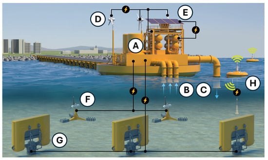
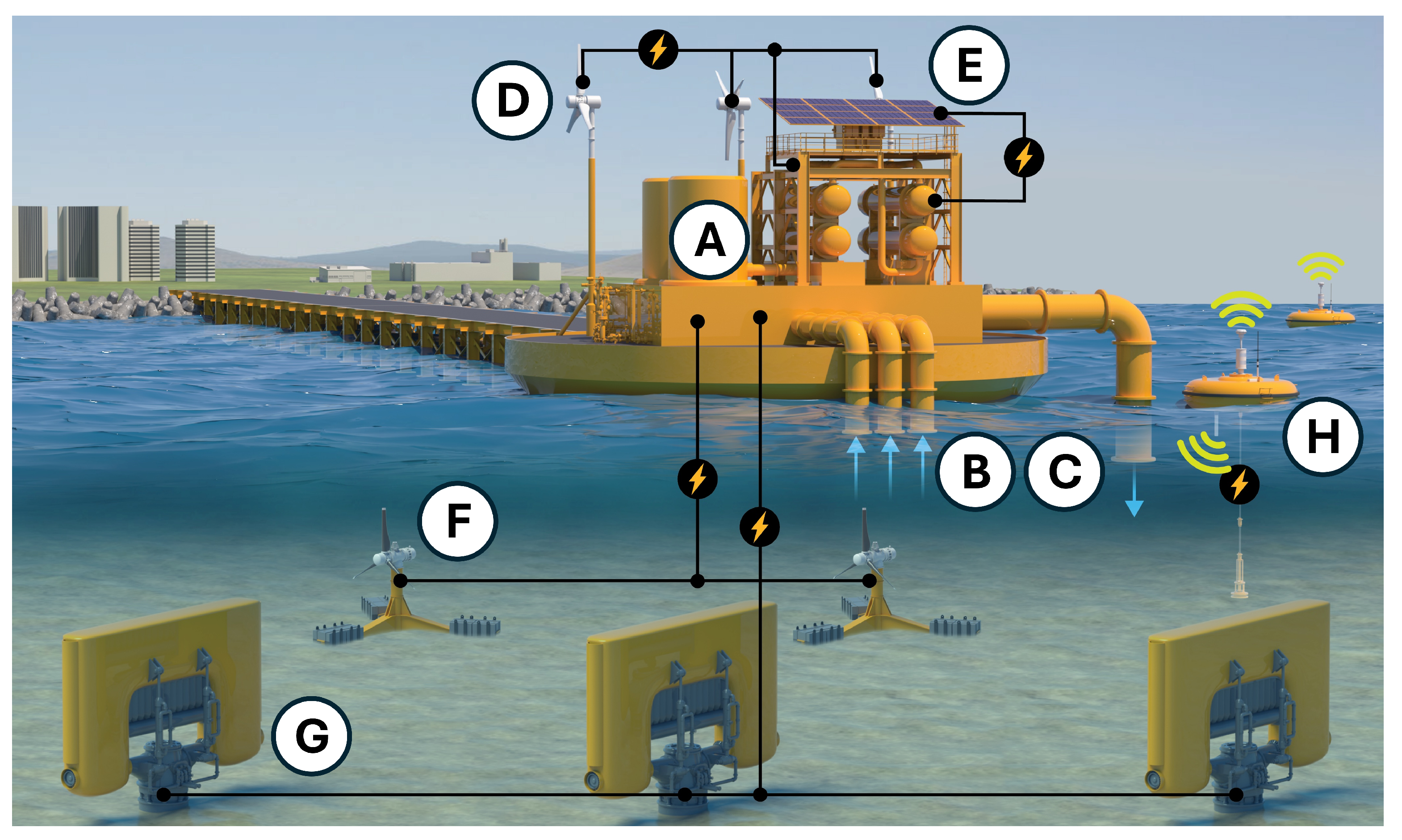
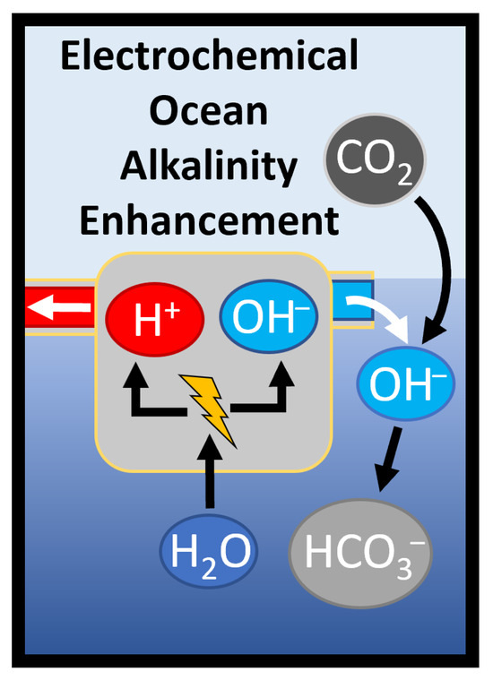
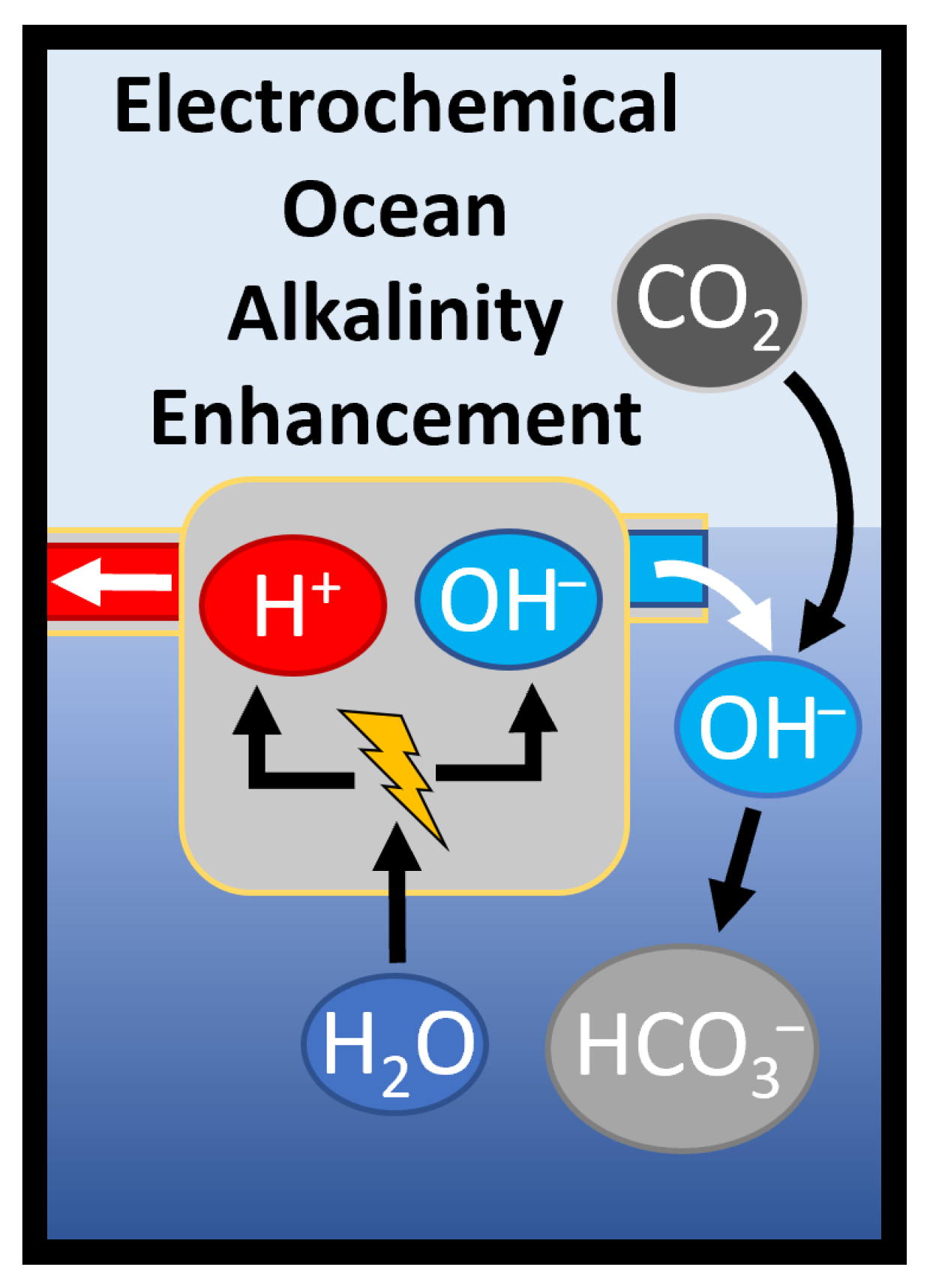
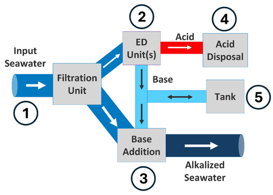
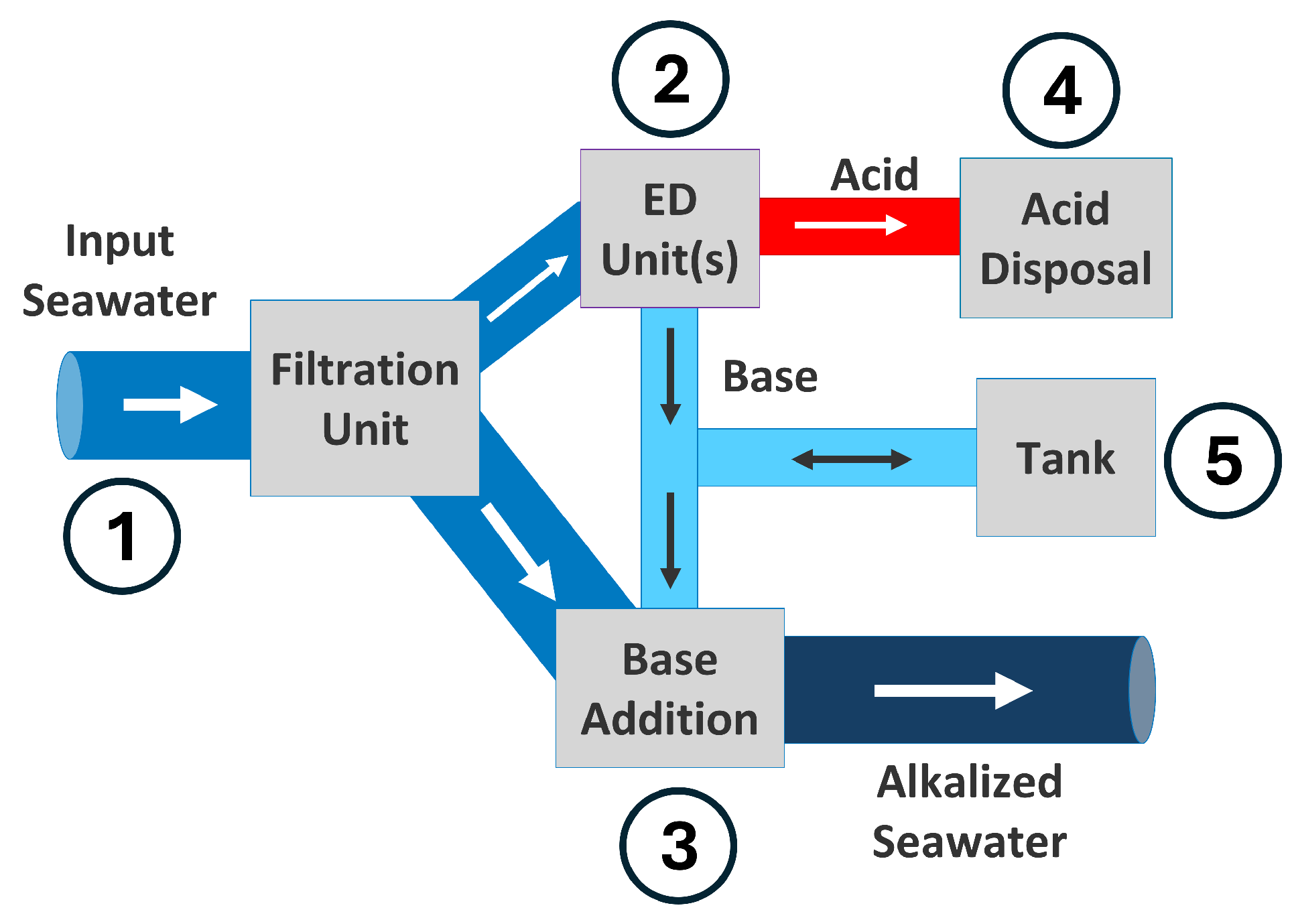
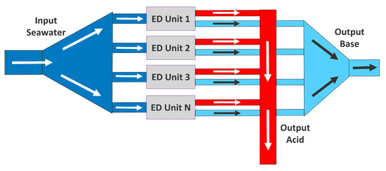
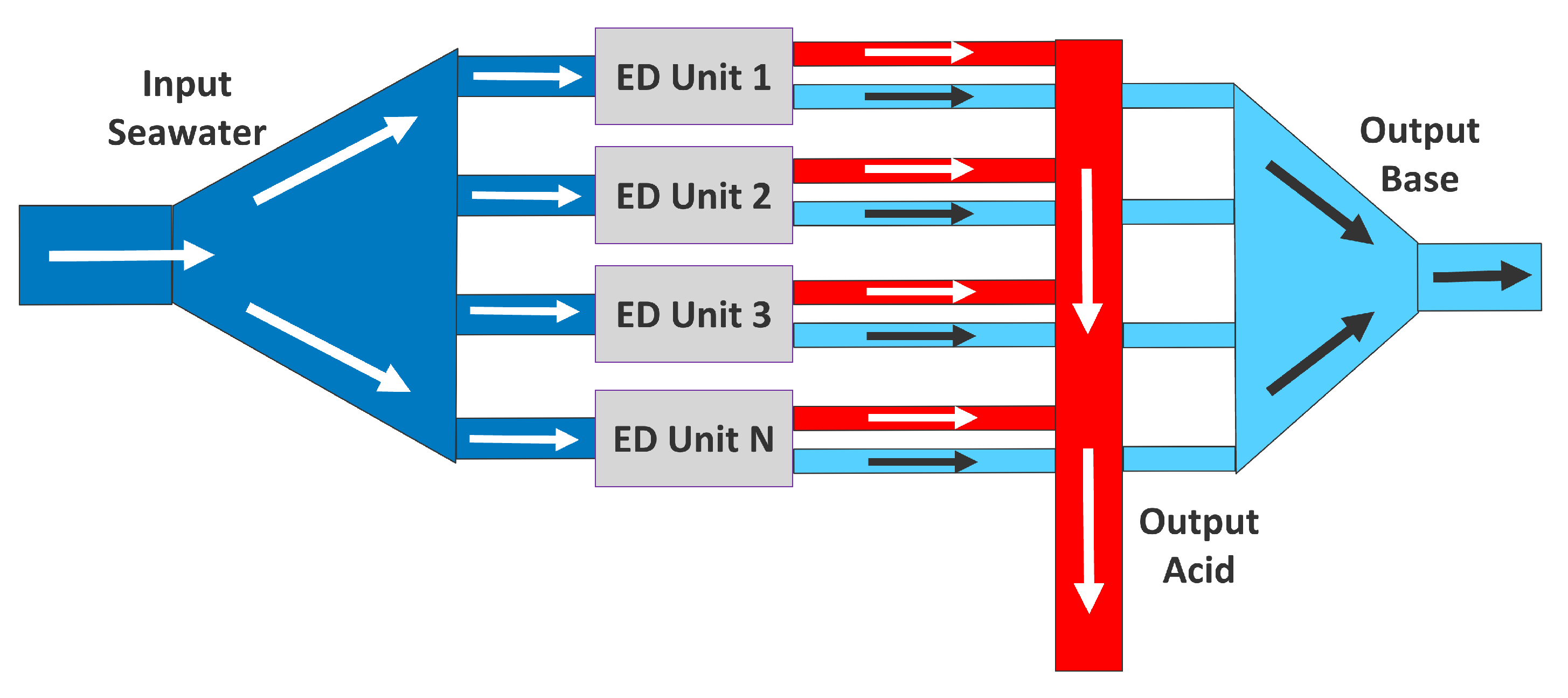
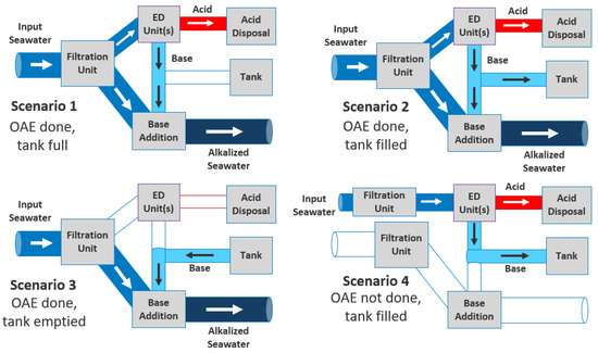
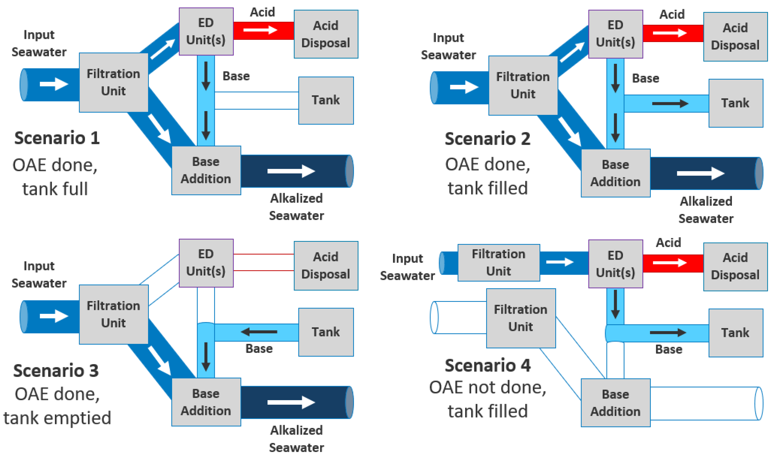
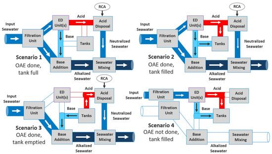
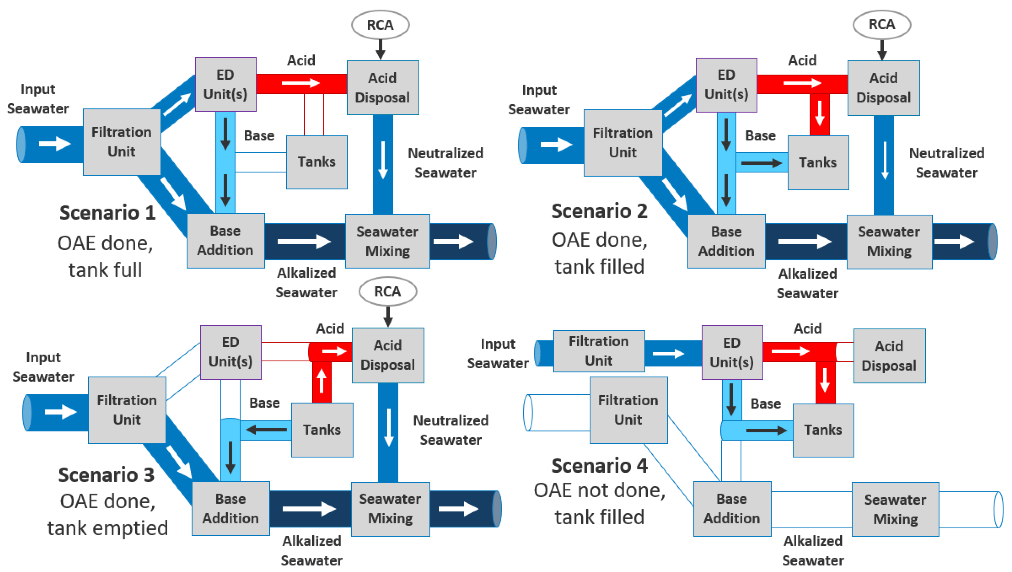
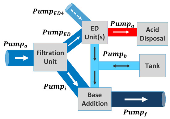
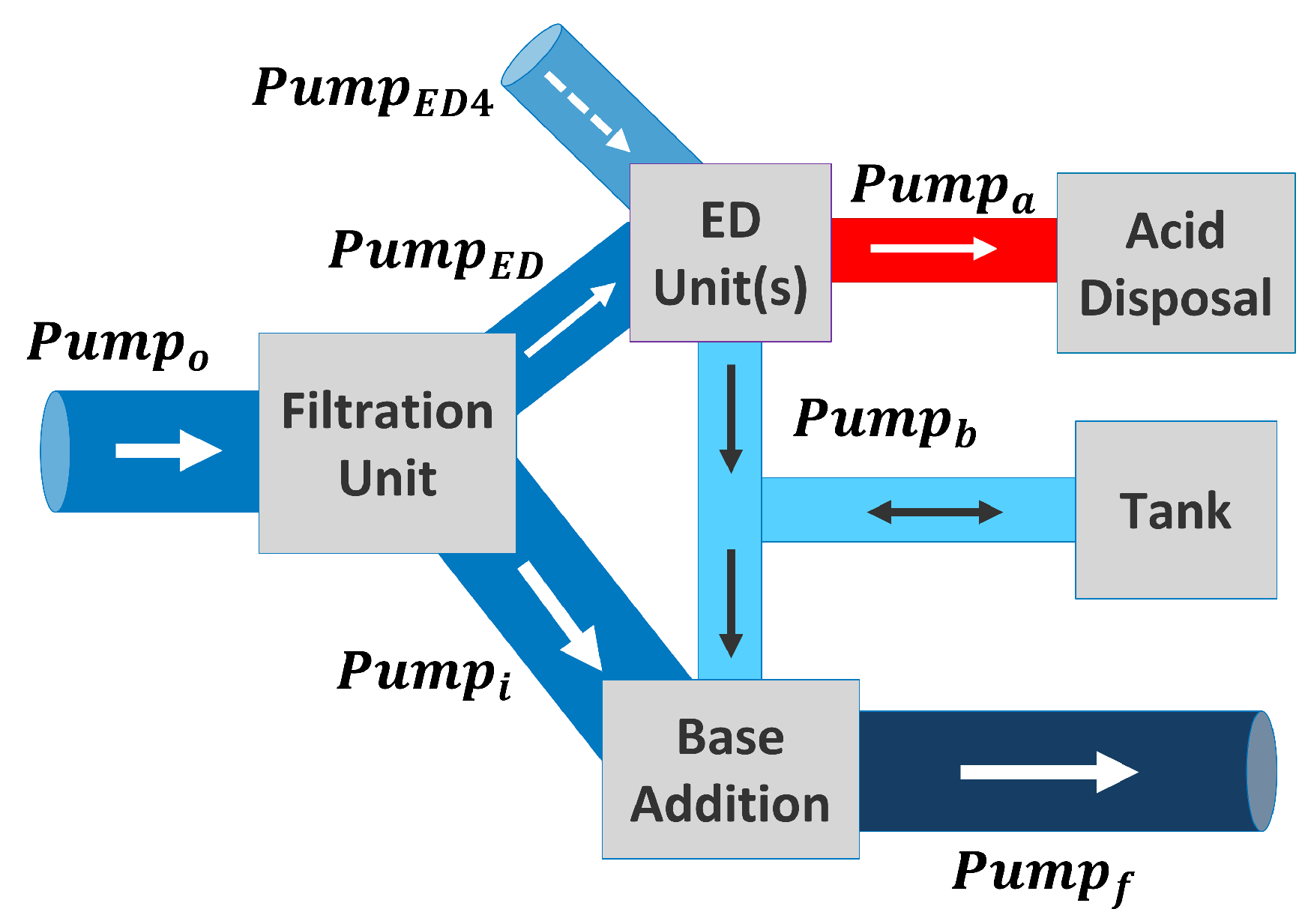
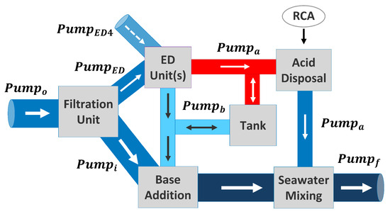
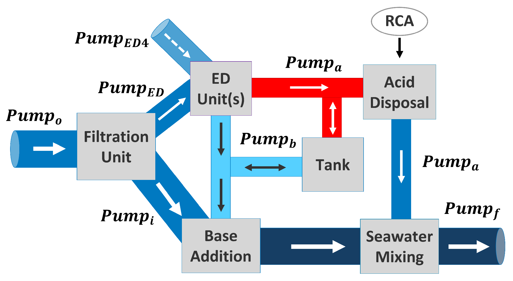
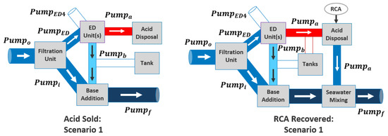
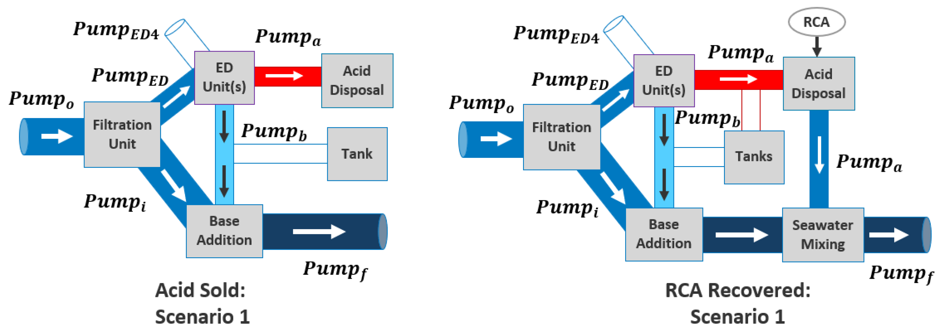
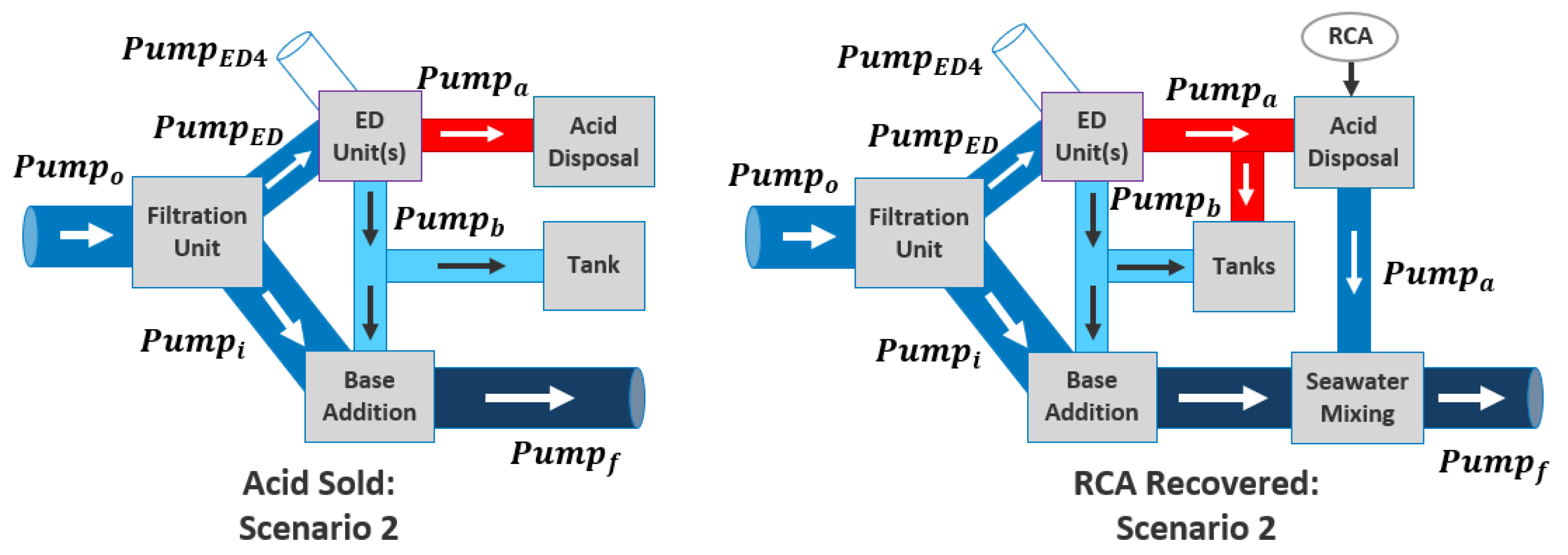
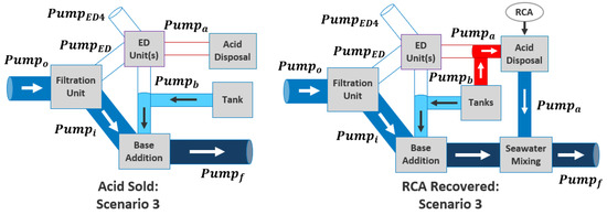
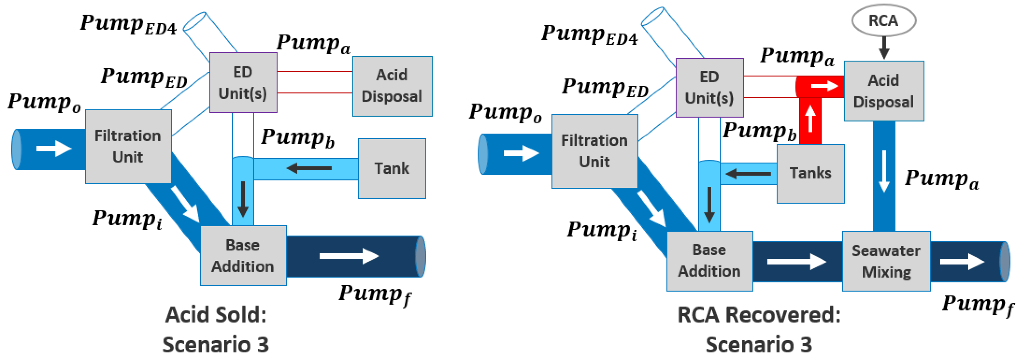
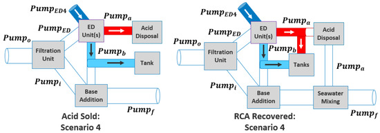
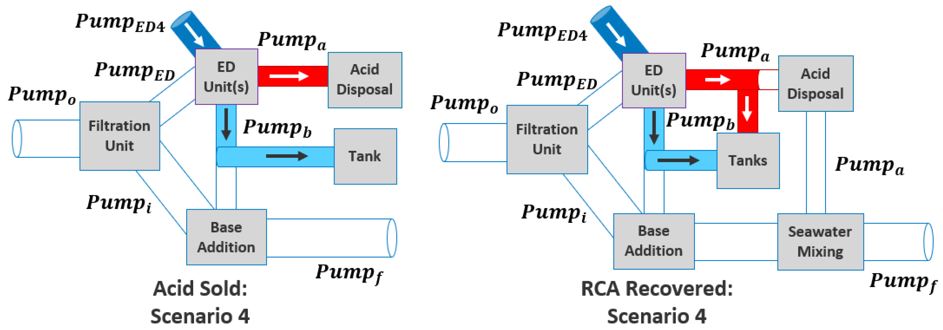
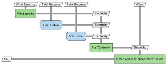
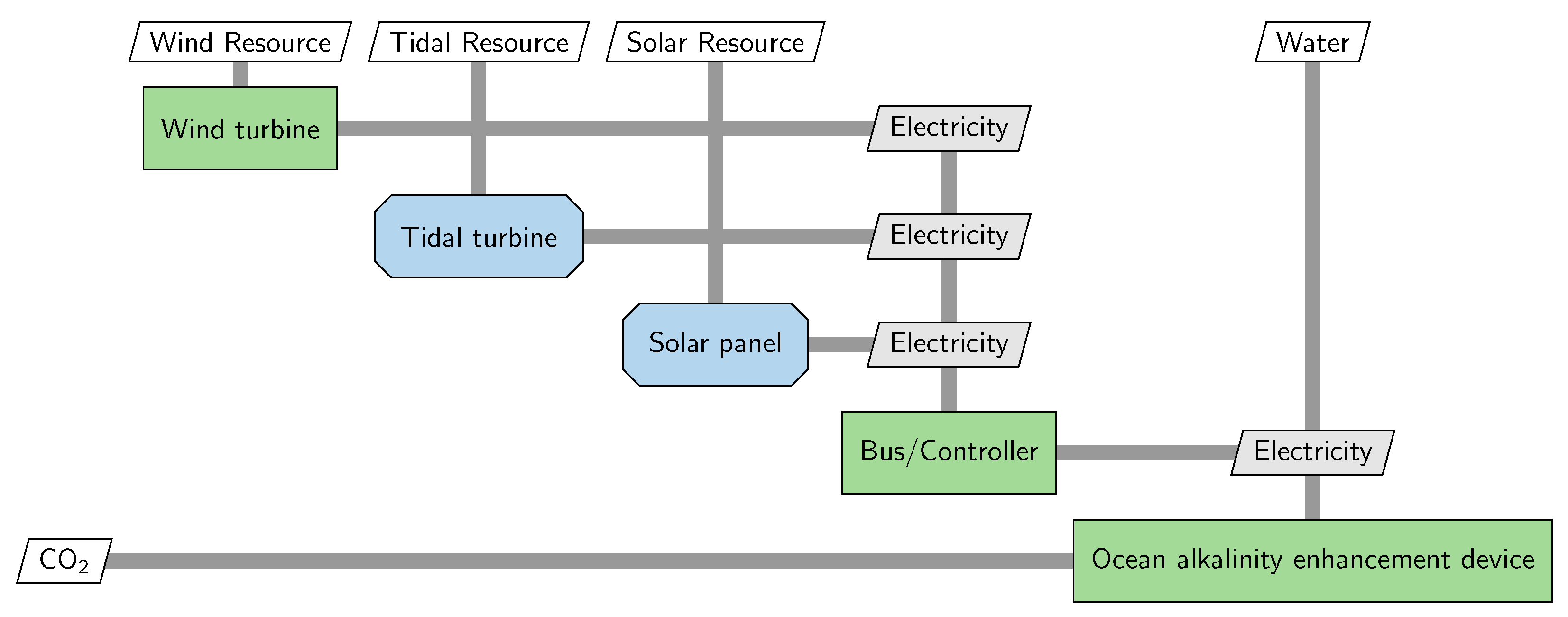
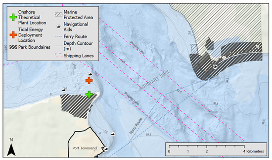
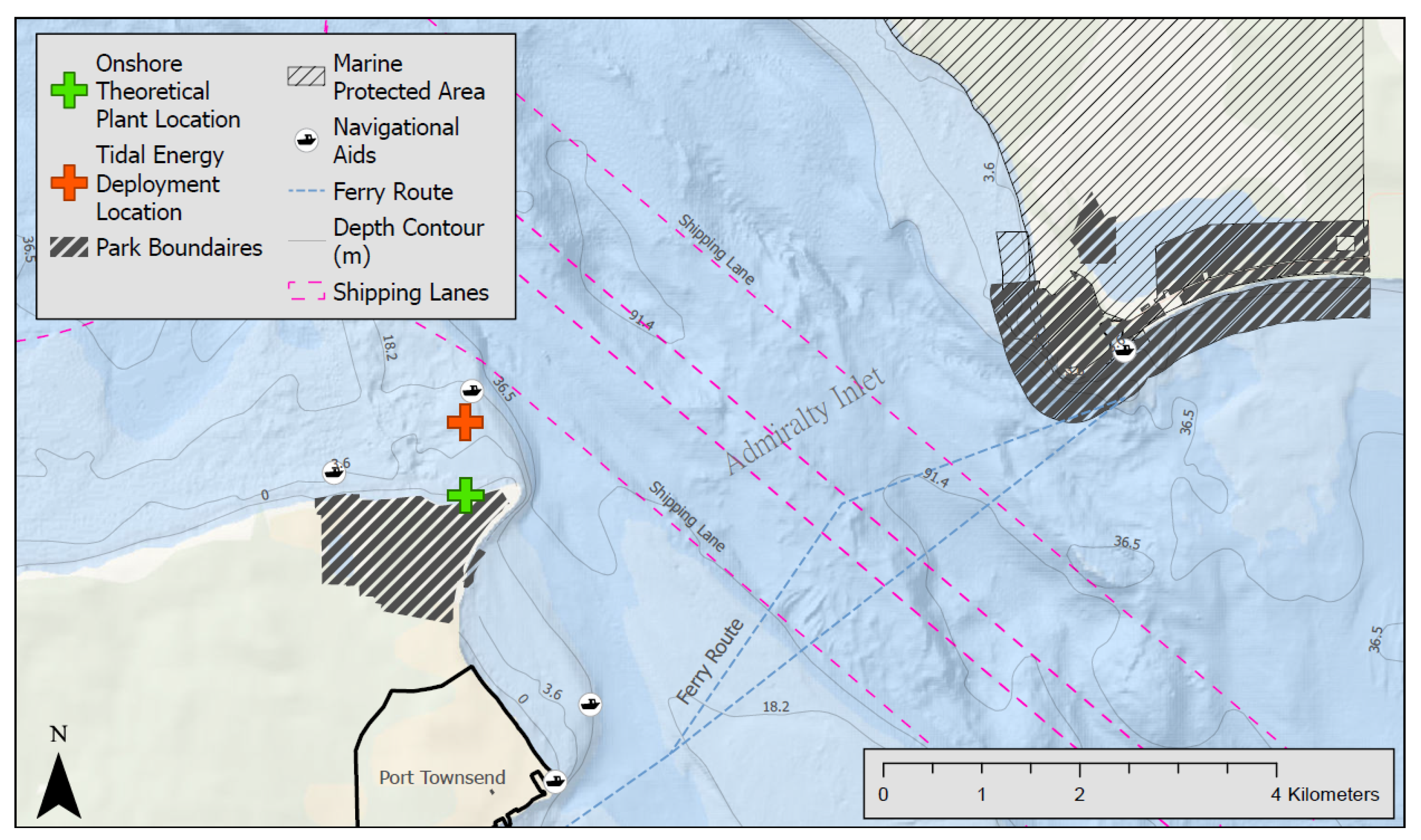
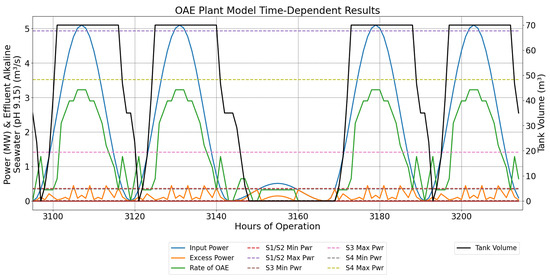
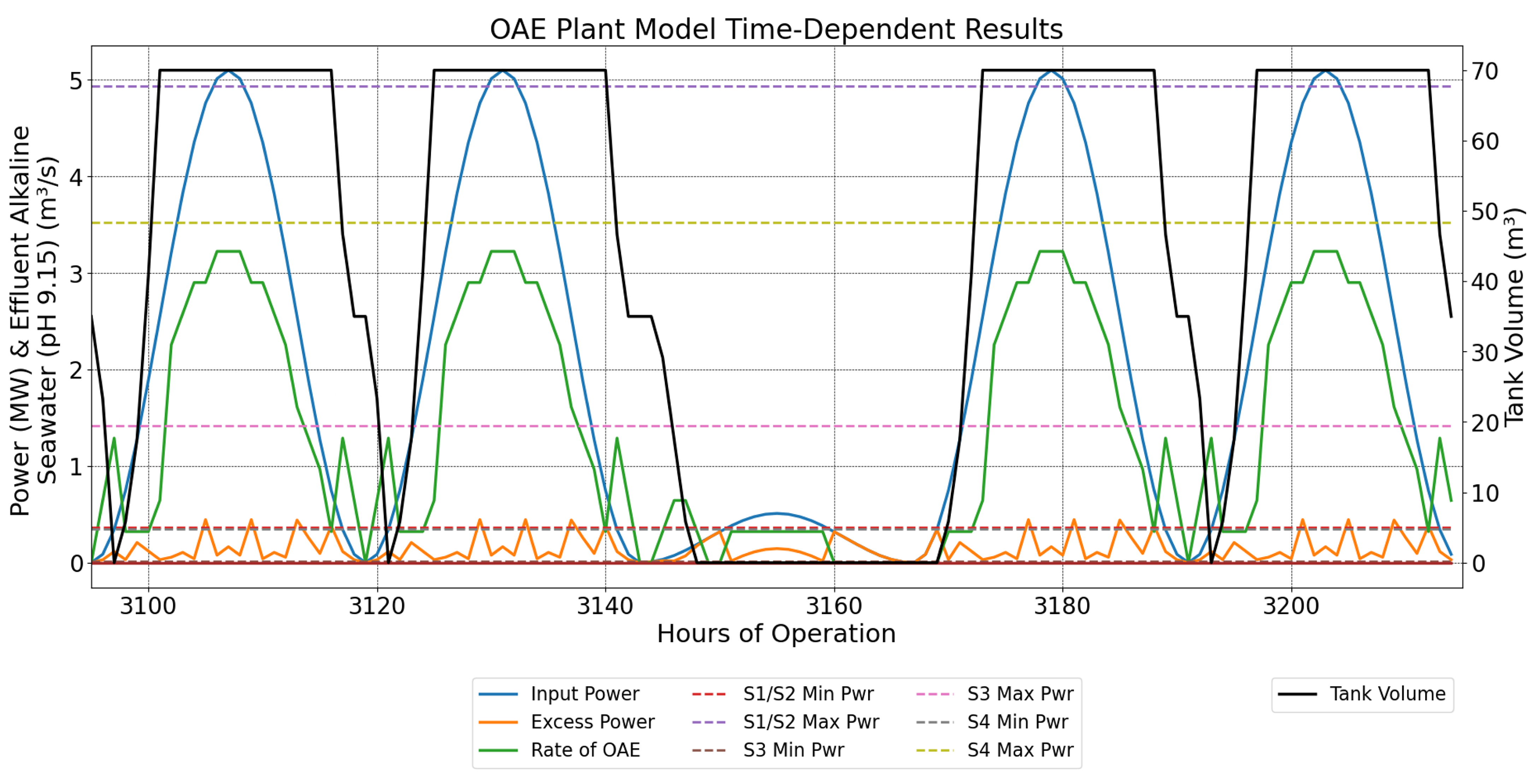
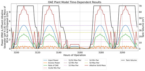
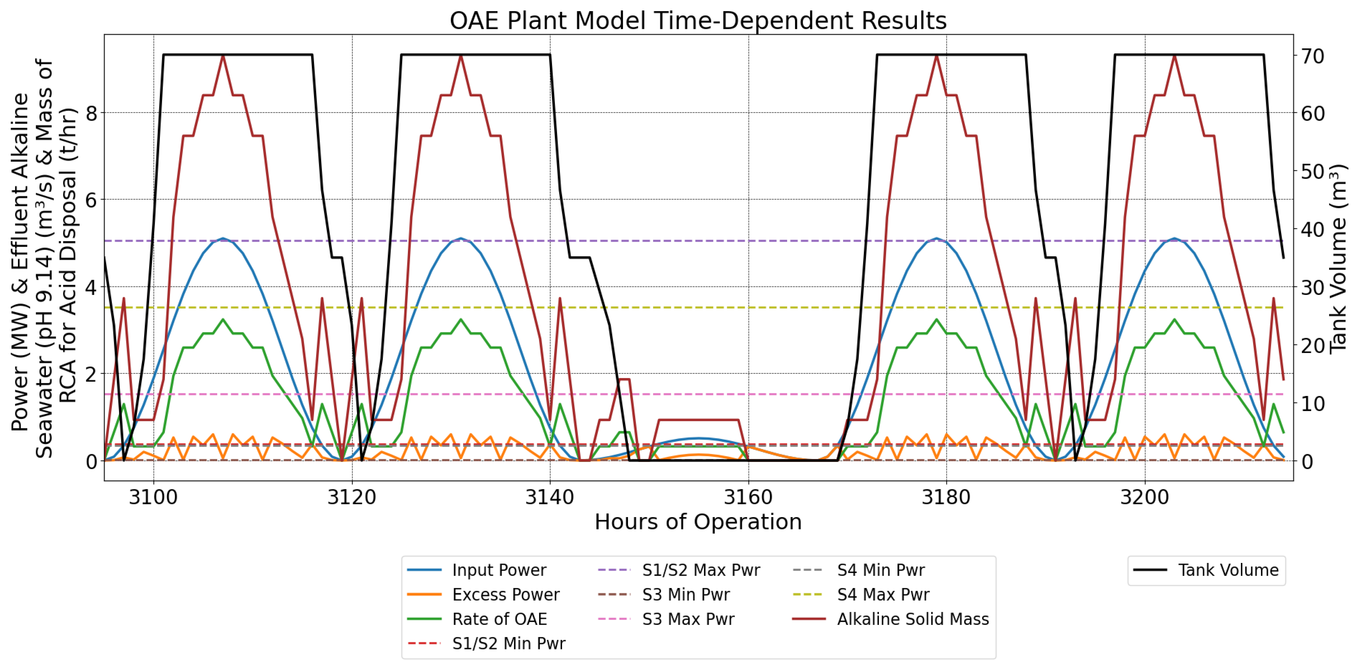
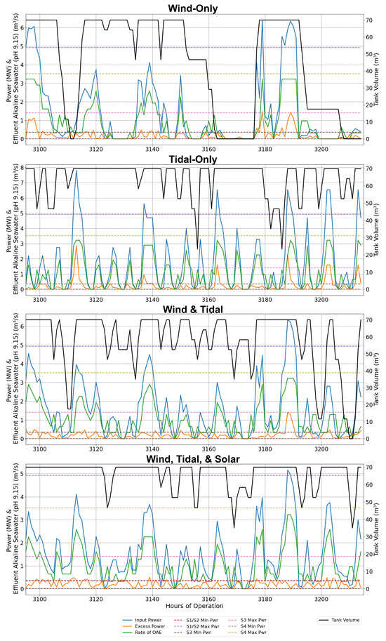
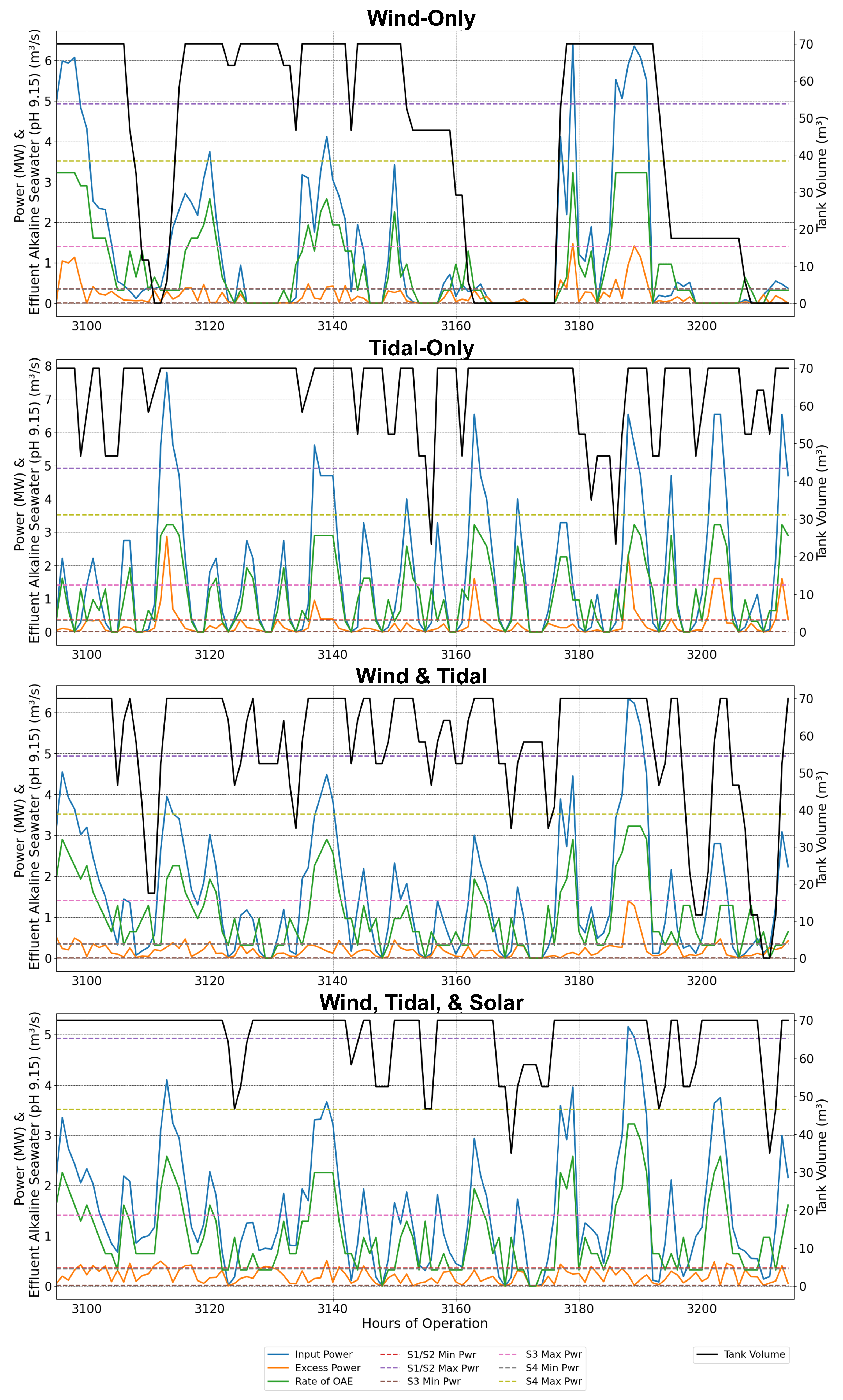
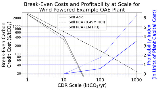
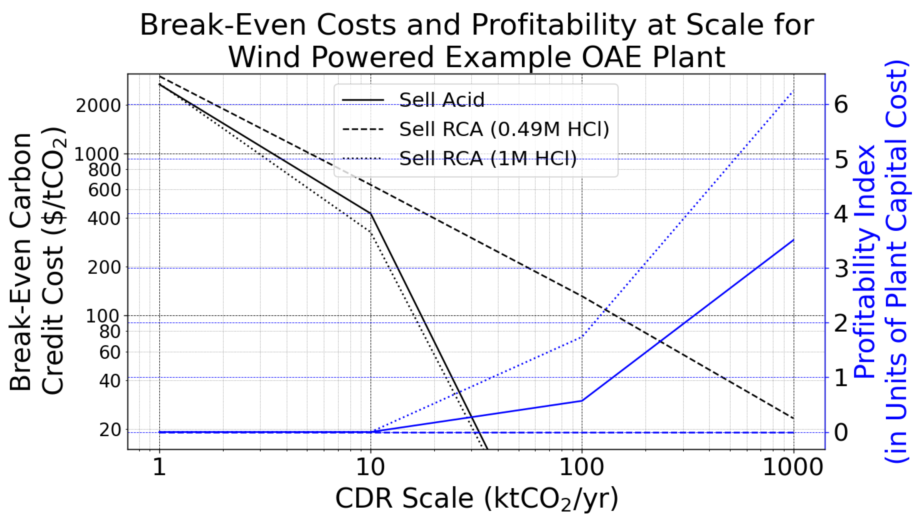
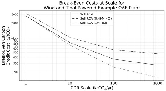
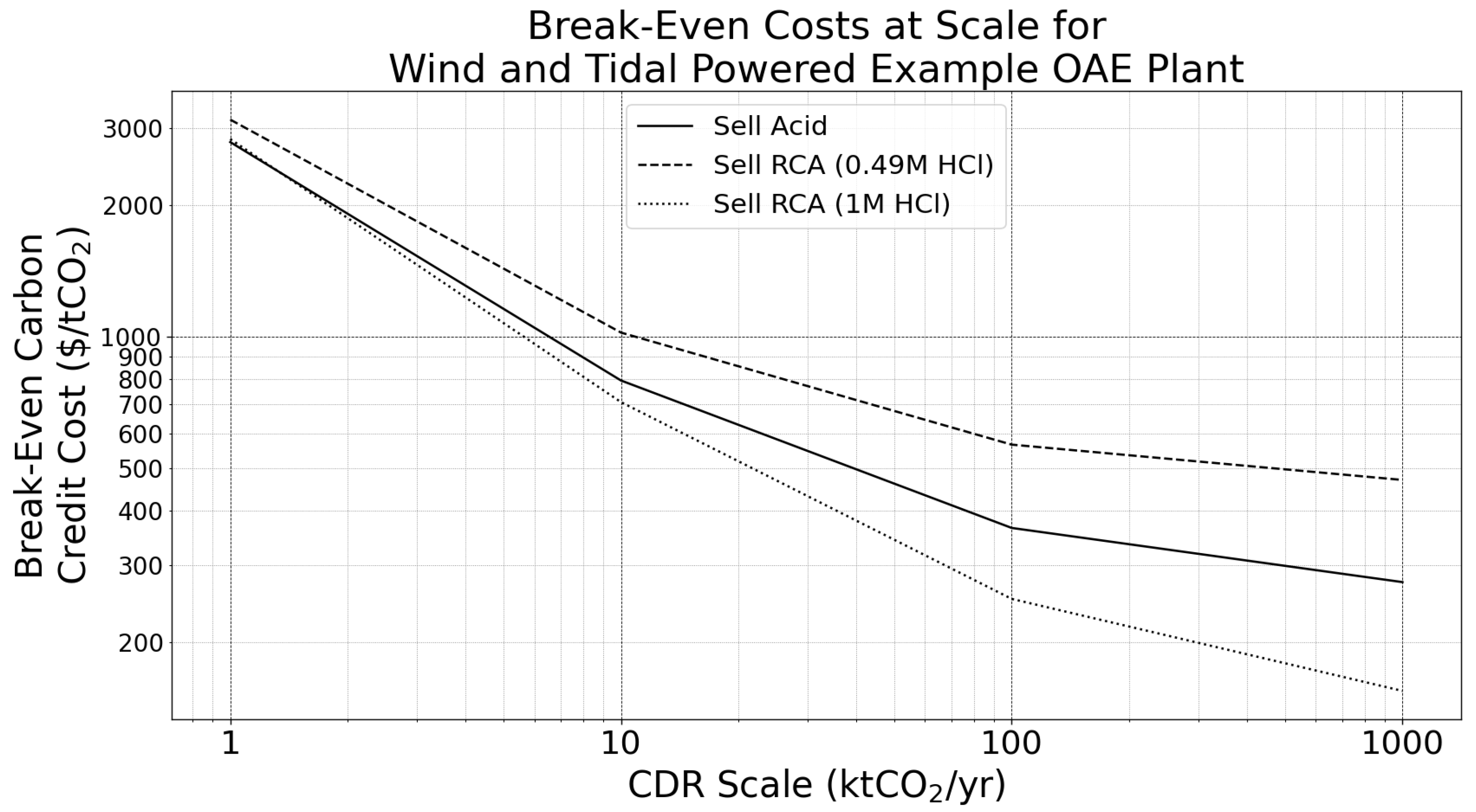

Disclaimer/Publisher’s Note: The statements, opinions and data contained in all publications are solely those of the individual author(s) and contributor(s) and not of MDPI and/or the editor(s). MDPI and/or the editor(s) disclaim responsibility for any injury to people or property resulting from any ideas, methods, instructions or products referred to in the content. |
© 2026 by the authors. Licensee MDPI, Basel, Switzerland. This article is an open access article distributed under the terms and conditions of the Creative Commons Attribution (CC BY) license.