Free Vibrations of Multi-Degree Structures: Solving Quadratic Eigenvalue Problems with an Excitation and Fast Iterative Detection Method

Abstract

For the free vibrations of multi-degree mechanical structures appeared in structural dynamics, we solve the quadratic eigenvalue problem either by linearizing it to a generalized eigenvalue problem or directly treating it by developing the iterative detection methods for the real and complex eigenvalues. To solve the generalized eigenvalue problem, we impose a nonzero exciting vector into the eigen-equation, and solve a nonhomogeneous linear system to obtain a response curve, which consists of the magnitudes of the n-vectors with respect to the eigen-parameters in a range. The n-dimensional eigenvector is supposed to be a superposition of a constant exciting vector and an m-vector, which can be obtained in terms of eigen-parameter by solving the projected eigen-equation. In doing so, we can save computational cost because the response curve is generated from the data acquired in a lower dimensional subspace. We develop a fast iterative detection method by maximizing the magnitude to locate the eigenvalue, which appears as a peak in the response curve. Through zoom-in sequentially, very accurate eigenvalue can be obtained. We reduce the number of eigen-equation to $n-1$ to find the eigen-mode with its certain component being normalized to the unit. The real and complex eigenvalues and eigen-modes can be determined simultaneously, quickly and accurately by the proposed methods.

1. Introduction

In the free vibration of a q-degree mass-damping-spring structure, the system of differential equations for describing the motion is [1]

$$\mathbf{M}\ddot{\mathbf{q}}\left(t\right)+\mathbf{C}\dot{\mathbf{q}}\left(t\right)+\mathbf{K}\mathbf{q}\left(t\right)=\mathbf{0},$$

(1)

where $\mathbf{q}\left(t\right)$ is a time-dependent q-dimensional vector to signify the generalized displacements of the system.

In engineering application the mass matrix $\mathbf{M}$ and the stiffness matrix $\mathbf{K}$ are positive definite because they are related to the kinetic energy and elastic strain energy. However, the damping properties of a system reflected in the viscous damping matrix $\mathbf{C}$ are rarely known, making it difficult to be evaluated exactly [2,3].

In terms of the vibration mode $\mathbf{u}$, we can express the fundamental solution of Equation (1) as

$$\mathbf{q}\left(t\right)=e^{\lambda t}\mathbf{u},$$

(2)

which leads to a nonlinear eigen-equation for $(\lambda ,\mathbf{u})$:

$$\mathbf{Q}\left(\lambda \right)\mathbf{u}:=({\lambda }^2\mathbf{M}+\lambda \mathbf{C}+\mathbf{K})\mathbf{u}=\mathbf{0},$$

(3)

where $\mathbf{Q}\left(\lambda \right)$ is a matrix quadratic of the structure. Equation (3) is a quadratic eigenvalue problem (QEP) to determine the eigen-pair $(\lambda ,\mathbf{u})$. In addition to the free vibrations of mechanical structures, many related systems which lead to the quadratic eigenvalue problems were discussed by Tisseur and Meerbergen [4]. In the design of linear structure, knowing natural frequency of the structure is vital important to avoid the resonance with external exciting. The natural frequency is the imaginary part of the eigenvalue $\lambda$ in Equation (3), which is a frequency to easily vibrate the structure [5,6].

Using the generalized Bezout method [7] to tackle Equation (3) one introduces a solvent matrix $\mathbf{S}$ determined by

$$\mathbf{Q}\left(\mathbf{S}\right)=\mathbf{M}{\mathbf{S}}^2+\mathbf{C}\mathbf{S}+\mathbf{K}={\mathbf{0}}_q,$$

(4)

where ${\mathbf{0}}_q$ is a $q\times q$ zero matrix, such that a factorization of $\mathbf{Q}\left(\lambda \right)$ reads as

$$\mathbf{Q}\left(\lambda \right)=(\lambda \mathbf{M}+\mathbf{M}\mathbf{S}+\mathbf{C})(\lambda {\mathbf{I}}_q-\mathbf{S}).$$

(5)

It gives us an opportunity to determine the eigenvalues of Equation (3) through the eigenvalues solved from two q-dimensional eigenvalue problems, generalized one and standard one:

$$(\mathbf{M}\mathbf{S}+\mathbf{C})\mathbf{u}=-\lambda \mathbf{M}\mathbf{u},\mathbf{S}\mathbf{u}=\lambda \mathbf{u}.$$

(6)

The key point of the solvent matrix method is solving a nonlinear matrix Equation (4) to obtain an accurate matrix $\mathbf{S}$ [8,9]. Most of the numerical methods that deal directly with the quadratic eigenvalue problem by solving Equations (4) and (6) are the variants of Newton’s method [10,11,12,13]. These Newton’s variants converge when the initial guess is close enough to the solution. But even for a good initial guess there is no guarantee that the method will converge to the desired eigenvalue. There are different methods to solve the quadratic eigenvalue problems [14,15,16,17,18,19].

Let

$$\mathbf{v}=\lambda \mathbf{u}$$

(7)

be the generalized velocity of vibration mode. We can combine Equations (7) and (3) together as

$$\left[\begin{array}{cc}{\mathbf{0}}_q& {\mathbf{I}}_q\\ -\mathbf{K}& -\mathbf{C}\end{array}\right]\left[\begin{array}{c}\mathbf{u}\\ \mathbf{v}\end{array}\right]=\lambda \left[\begin{array}{cc}{\mathbf{I}}_q& {\mathbf{0}}_q\\ {\mathbf{0}}_q& \mathbf{M}\end{array}\right]\left[\begin{array}{c}\mathbf{u}\\ \mathbf{v}\end{array}\right].$$

(8)

Defining

$$\mathbf{x}:=\left[\begin{array}{c}\mathbf{u}\\ \mathbf{v}\end{array}\right],\mathbf{A}:=\left[\begin{array}{cc}{\mathbf{0}}_q& {\mathbf{I}}_q\\ -\mathbf{K}& -\mathbf{C}\end{array}\right],\mathbf{B}:=\left[\begin{array}{cc}{\mathbf{I}}_q& {\mathbf{0}}_q\\ {\mathbf{0}}_q& \mathbf{M}\end{array}\right],$$

(9)

Equation (8) becomes a generalized eigenvalue problem for the n-vector $\mathbf{x}$:

$$\mathbf{A}\mathbf{x}=\lambda \mathbf{B}\mathbf{x},$$

(10)

where $\mathbf{A},\mathbf{B}\in {\mathbb{R}}^{n\times n}$ with $n=2q$. Equation (10) is used to determine the eigen-pair $(\lambda ,\mathbf{x})$, which is a linear eigen-equation associated to the pencil $\mathbf{A}-\lambda \mathbf{B}$, where $\lambda$ is an eigen-parameter.

In the linearization from Equation (3) to Equation (10), an unsatisfactory aspect is that the dimension of the working space is doubled to $n=2q$. However, for the generalized eigenvalue problems many powerful numerical methods are available [20,21]. The numerical computations in [22,23] revealed that the methods based on the Krylov subspace can be very effective in the nonsymmetric eigenvalue problems by using the Lanczos biorthogonalization algorithm and the Arnoldi’s algorithm. The Arnoldi and nonsymmetric Lanczos methods are both of the Krylov subspace methods. Among the many algorithms to solve the matrix eigenvalue problems the Arnoldi method [23,24,25,26], the nonsymmetric Lanczos algorithm [27], and the subspace iteration method [28] are well known. The affine Krylov subspace method was first developed by Liu [29] to solve linear equations system, which is however not yet used to solve the generalized eigenvalue problems. It is well known that the eig function in MATLAB is an effective code to compute the eigenvalues of the generalized eigenvalue problems. We will test it for the eigenvalue problem of highly ill-conditioned matrices and point out its limitation.

The paper sets up a new detection method for determining the real and complex eigenvalues of Equation (10) in Section 2, where the idea of exciting vector and excitation method (EM) are introduced with two examples being demonstrated. In Section 3, we express the generalized eigenvalue problem (10) in an affine Krylov subspace, and a nonhomogeneous linear equations system is derived. To precisely locate the position of the real eigenvalue in the response curve, we develop an iterative detection method (IDM) in Section 4, where we derive new methods to compute eigenvalue and eigenvector. In Section 5 some examples of the generalized eigenvalue problems are given. The EM and IDM are extended in Section 6 to directly solve the quadratic eigenvalue problem (3), where we derive IDM in the eigen-parametric plane to determine the complex eigenvalue. In Section 7, several examples are given and solved by either linearizing them to the generalized eigenvalue problems or treating them in the original quadratic forms by the direct detection method. Finally, the conclusions are drawn in Section 8.

2. A New Detection Method

Let $\lambda (\mathbf{A},\mathbf{B})$ be the set of all the eigenvalues of Equation (10), which may include the pairs of conjugate complex eigenvalues. It is known that if $\lambda \notin \lambda (\mathbf{A},\mathbf{B})$ then Equation (10) has only the trivial solution with $\mathbf{x}=\mathbf{0}$ and $\parallel \mathbf{x}\parallel =0$. In contrast, if $\lambda \in \lambda (\mathbf{A},\mathbf{B})$ then Equation (10) has a non-trivial solution with $\mathbf{x}\ne \mathbf{0}$ and $\parallel \mathbf{x}\parallel >0$, which is called the eigenvector. However, when n is large it is difficult to directly solve Equation (10) to determine $\lambda$ and $\mathbf{x}$ by the manual operations. Instead, numerical methods have to be employed to solve Equation (10), from which $\mathbf{x}$ is always obtained to be a zero vector no matter which $\lambda$ is, since the right-hand side of $(\mathbf{A}-\lambda \mathbf{B})\mathbf{x}=\mathbf{0}$ is zero.

To definitely determine $\mathbf{x}$ to have a finite magnitude with $0\le \parallel \mathbf{x}\parallel <\infty$, we consider a variable transformation from $\mathbf{x}$ to $\mathbf{y}$ by

$$\mathbf{x}={\mathbf{x}}_0+\mathbf{y},$$

(11)

where ${\mathbf{x}}_0$ is a given nonzero vector, which being inserted into Equation (10) generates

$$(\mathbf{A}-\lambda \mathbf{B})\mathbf{y}=-(\mathbf{A}-\lambda \mathbf{B}){\mathbf{x}}_0.$$

(12)

It is important that the right-hand side is not zero because of ${\mathbf{x}}_0\ne \mathbf{0}$, which is a given exciting vector to render a nonzero response of $\mathbf{y}\ne \mathbf{0}$ and then $\mathbf{x}\ne \mathbf{0}$ by Equation (11) is available. We must emphasize that when $\mathbf{A}-\lambda \mathbf{B}$ is near to a singular matrix, we cannot eliminate $\mathbf{A}-\lambda \mathbf{B}$ in Equation (12) by inverting the matrix $\mathbf{A}-\lambda \mathbf{B}$ to obtain $\mathbf{y}=-{\mathbf{x}}_0$.

2.1. Real Eigenvalue

Let the eigen-parameter in Equation (12) run in an interval $\lambda \in [a,b]$, and we can solve Equation (12) by the Gaussian elimination method to obtain $\mathbf{y}$ and then $\mathbf{x}={\mathbf{x}}_0+\mathbf{y}$. Hence, the response curve is formed by varying the magnitude $\parallel \mathbf{x}\left(\lambda \right)\parallel$ vs. the eigen-parameter $\lambda$ in the interval $\lambda \in [a,b]$. It is different from Equation (10) that now we can compute $\mathbf{y}$ in Equation (12) and then $\mathbf{x}$ by Equation (11), when ${\mathbf{x}}_0$ is a given nonzero vector. Through this transformation by solving a nonhomogeneous linear system (12), rather than the homogeneous linear system (10), the resultant vector $\mathbf{x}$ can generate a nonzero finite response of $\parallel \mathbf{x}\parallel$ when the eigen-parameter tends to an eigenvalue, and for most eigen-parameters that not near to any eigenvalue the responses of $\parallel \mathbf{x}\parallel$ are very small, nearly close to zero. The technique to construct a nonzero response curve is called an excitation method (EM).

For instance, we consider Equation (10) endowing with [20]:

$$\mathbf{A}=\left[\begin{array}{ccccc}2& 3& 4& 5& 6\\ 4& 4& 5& 6& 7\\ 0& 3& 6& 7& 8\\ 0& 0& 2& 8& 9\\ 0& 0& 0& 1& 10\end{array}\right],\mathbf{B}=\left[\begin{array}{ccccc}1& -1& -1& -1& -1\\ 0& 1& -1& -1& -1\\ 0& 0& 1& -1& -1\\ 0& 0& 0& 1& -1\\ 0& 0& 0& 0& 1\end{array}\right].$$

(13)

We take $[a,b]=[-5,25]$ and ${\mathbf{x}}_0=\mathbf{0}$, and we plot $\parallel \mathbf{x}\left(\lambda \right)\parallel$ vs. the eigen-parameter $\lambda \in [-5,25]$ in Figure 1a, wherein only zero values of $\parallel \mathbf{x}\left(\lambda \right)\parallel$ appear.

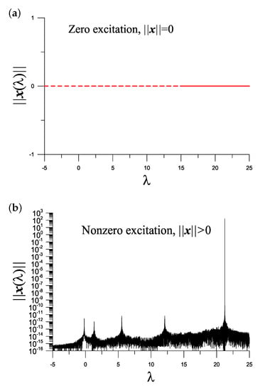
Figure 1. For a generalized eigenvalue problem (13), (a) zero response under a zero excitation, and (b) showing five peaks in the response curve under a nonzero excitation.

However, under a nonzero excitation with ${\mathbf{x}}_0={\mathbf{1}}_5:={(1,1,1,1,1)}^T$, we plot $\parallel \mathbf{x}\left(\lambda \right)\parallel$ vs. the eigen-parameter $\lambda \in [-5,25]$ in Figure 1b, where we can observe five peaks of the response curve which signifying the locations of five real eigenvalues to be sought. When $\lambda$ does not locate at the peak point, $\parallel \mathbf{x}\left(\lambda \right)\parallel$ is zero from the theoretical point of view; however, the value of $\parallel \mathbf{x}\left(\lambda \right)\parallel$ as shown in Figure 1b is not zero, which is very small due to the machinery round-off error caused by using the Gaussian elimination method to solve Equation (12). In Section 4, we will develop an iterative method to precisely locate those eigenvalues based on the EM.

2.2. Complex Eigenvalue

Because $\mathbf{A}$ and $\mathbf{B}$ are real matrices, the eigenvalue may be a complex number, which is assumed to be

$$\lambda ={\lambda }_R+i{\lambda }_I,$$

(14)

where $i^2=-1$, and ${\lambda }_R$ and ${\lambda }_I$ are, respectively, the real and imaginary parts of $\lambda$. Correspondingly, we take

$$\mathbf{x}=\mathbf{z}+i\mathbf{w}.$$

(15)

Inserting Equations (14) and (15) into Equation (10), yields

$$\left[\begin{array}{cc}\mathbf{A}-{\lambda }_R\mathbf{B}& {\lambda }_I\mathbf{B}\\ -{\lambda }_I\mathbf{B}& \mathbf{A}-{\lambda }_R\mathbf{B}\end{array}\right]\left[\begin{array}{c}\mathbf{z}\\ \mathbf{w}\end{array}\right]=\mathbf{0}.$$

(16)

Letting

$$\mathbf{X}:=\left[\begin{array}{c}\mathbf{z}\\ \mathbf{w}\end{array}\right],\mathbf{D}:=\left[\begin{array}{cc}\mathbf{A}-{\lambda }_R\mathbf{B}& {\lambda }_I\mathbf{B}\\ -{\lambda }_I\mathbf{B}& \mathbf{A}-{\lambda }_R\mathbf{B}\end{array}\right],$$

(17)

Equation (16) becomes

$$\mathbf{D}\mathbf{X}=\mathbf{0}.$$

(18)

Similarly, by taking

$$\mathbf{X}={\mathbf{X}}_0+\mathbf{Y},$$

(19)

where ${\mathbf{X}}_0\ne \mathbf{0}$ is a given exciting vector and by Equation (18), we have

$$\mathbf{D}\mathbf{Y}=-\mathbf{D}{\mathbf{X}}_0.$$

(20)

No matter which $\mathbf{D}$ is, since Equation (20) is a consistent linear system with a dimension $2n$, we can solve it by using the Gaussian elimination method to obtain $\mathbf{Y}$ and then $\mathbf{X}$ by Equation (19).

When ${\lambda }_R$ and ${\lambda }_I$ take values inside a rectangle by $({\lambda }_R,{\lambda }_I)\in [a,b]\times [c,d]$, we can plot $\parallel \mathbf{X}({\lambda }_R,{\lambda }_I)\parallel$ vs. $({\lambda }_R,{\lambda }_I)$ over the eigen-parametric plane, and investigate the property of the response surface.

For instance, for

$$\mathbf{A}=\left[\begin{array}{cc}1& -1\\ 1& 2\end{array}\right],\mathbf{B}=\left[\begin{array}{cc}1& 0\\ 0& 1\end{array}\right],$$

(21)

we have a pair of complex eigenvalues:

$$\lambda =\frac{3}{2}\pm \frac{i\sqrt{3}}{2}.$$

(22)

We take $[a,b]=[1,2]$, $[c,d]=[0,1]$, and with ${\mathbf{X}}_0={\mathbf{1}}_4$, we plot $\parallel \mathbf{X}({\lambda }_R,{\lambda }_I)\parallel$ over the plane $({\lambda }_R,{\lambda }_I)$ in Figure 2, where we can observe one peak near to the point $(3/2,\sqrt{3}/2)$. More precise values of $({\lambda }_R,{\lambda }_I)$ will be obtained by the iterative detection method to be developed in Section 6.

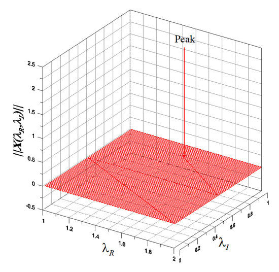
Figure 2. For a 2 by 2 matrix the detection of a complex eigenvalue.

3. Generalized Eigenvalue Problem in an Affine Krylov Subspace

The detection method developed in the previous section has a weakness that we need to solve an n-dimensional linear system (12) for real eigenvalue and a $2n$-dimensional linear system (20) for complex eigenvalue. Therefore, in the many selected points inside the range we may spend a lot of computational time to construct the response curve to detect real eigenvalues or the response surface to detect complex eigenvalues. In this section we develop the detection methods in a lower dimensional subspace, instead of the detection methods carried out in the full space.

3.1. The Krylov Subspace

When n is a large dimension, Equation (10) is a high-dimensional linear equations system. In order to reduce the dimension of the governing equation to m in an m-dimensional Krylov subspace, we begin with

$${\mathcal{K}}_m:=\mathrm{Span}\{\mathbf{A}{\mathbf{x}}_0,\dots ,{\mathbf{A}}^m{\mathbf{x}}_0\}.$$

(23)

The Krylov matrix is fixed by

$$\mathbf{U}:=[{\mathbf{u}}_1,\dots ,{\mathbf{u}}_m],$$

(24)

which is an $n\times m$ matrix with its jth column being the vector ${\mathbf{u}}_j$.

The Arnoldi process is used to normalize and orthogonalize the Krylov vectors ${\mathbf{A}}^j{\mathbf{x}}_0,j=1,\dots ,m$, such that the resultant vectors ${\mathbf{u}}_i,i=1,\dots ,m$ satisfy ${\mathbf{u}}_i·{\mathbf{u}}_j={\delta }_{ij},i,j=1,\dots ,m$, where ${\delta }_{ij}$ is the Kronecker delta symbol. The Arnoldi procedure for the orthogonalization of $\mathbf{U}$ can be written as follows [30].

$$\begin{array}{ccc}\hfill & & \mathrm{Select}m\mathrm{and\; give\; an\; initial\; vector}\mathbf{A}{\mathbf{x}}_0,\hfill \\ & & {\mathbf{u}}_1=\frac{\mathbf{A}{\mathbf{x}}_0}{\parallel \mathbf{A}{\mathbf{x}}_0\parallel },\hfill \\ & & \mathrm{Do}j=1:m-1,\hfill \\ & & {\mathbf{w}}_j=\mathbf{A}{\mathbf{u}}_j,\hfill \\ & & \mathrm{Do}i=1:j,\hfill \\ & & h_{ij}={\mathbf{u}}_i·{\mathbf{w}}_j,\hfill \\ & & {\mathbf{w}}_j={\mathbf{w}}_j-h_{ij}{\mathbf{u}}_i,\hfill \\ & & \mathrm{Enddo\; of}i,\hfill \\ & & h_{j+1,j}=\parallel {\mathbf{w}}_j\parallel .\mathrm{If}{h}_{j+1,j}=0\mathrm{stop},\hfill \\ & & {\mathbf{u}}_{j+1}=\frac{{\mathbf{w}}_j}{h_{j+1,j}},{\mathbf{U}}_{j+1}=\frac{{\mathbf{w}}_j}{h_{j+1,j}},\hfill \\ & & \mathrm{Enddo\; of}j.\hfill \end{array}$$

(25)

$\mathbf{U}$ denotes the Krylov matrix, where the subscript k in ${\mathbf{U}}_k$ means the kth column of $\mathbf{U}$, which possesses the following property:

$${\mathbf{U}}^{\mathrm{T}}\mathbf{U}={\mathbf{I}}_m.$$

(26)

3.2. Linear Nonhomogeneous Equations in an Affine Krylov Subspace

Because of $\mathbf{x}\in {\mathbf{x}}_0+{\mathcal{K}}_m$, we can expand $\mathbf{x}$ by

$$\mathbf{x}={\mathbf{x}}_0+\mathbf{U}\mathbf{\alpha },$$

(27)

where $\mathbf{\alpha }$ is an unknown m-vector to be determined. From Equations (10) and (27) it follows that

$$\mathbf{A}\mathbf{U}\mathbf{\alpha }+\mathbf{A}{\mathbf{x}}_0=\lambda \mathbf{B}\mathbf{U}\mathbf{\alpha }+\lambda \mathbf{B}{\mathbf{x}}_0,$$

(28)

which is projected onto the Krylov subspace ${\mathcal{K}}_m$ by

$${\mathbf{U}}^{\mathrm{T}}\mathbf{A}\mathbf{U}\mathbf{\alpha }+{\mathbf{U}}^{\mathrm{T}}\mathbf{A}{\mathbf{x}}_0=\lambda {\mathbf{U}}^{\mathrm{T}}\mathbf{B}\mathbf{U}\mathbf{\alpha }+\lambda {\mathbf{U}}^{\mathrm{T}}\mathbf{B}{\mathbf{x}}_0.$$

(29)

4. An Iterative Detection Method for Real Eigenvalue

It follows from Equation (29) that

$$\begin{array}{c}\hfill ({\mathbf{U}}^{\mathrm{T}}\mathbf{A}\mathbf{U}-\lambda {\mathbf{U}}^{\mathrm{T}}\mathbf{B}\mathbf{U})\mathbf{\alpha }=\lambda {\mathbf{U}}^{\mathrm{T}}\mathbf{B}{\mathbf{x}}_0-{\mathbf{U}}^{\mathrm{T}}\mathbf{A}{\mathbf{x}}_0,\end{array}$$

(30)

which is the projection of Equation (10) into the affine Krylov subspace ${\mathbf{x}}_0+{\mathcal{K}}_m$ as a nonhomogeneous projected eigen-equation. Upon comparing to the original eigen-equation $(\mathbf{A}-\lambda \mathbf{B})\mathbf{x}=\mathbf{0}$ in Equation (10), Equation (30) is different for the appearance of a nonhomogeneous term $\lambda {\mathbf{U}}^{\mathrm{T}}\mathbf{B}{\mathbf{x}}_0-{\mathbf{U}}^{\mathrm{T}}\mathbf{A}{\mathbf{x}}_0$ in the right-hand side, When we take ${\mathbf{x}}_0=\mathbf{0}$ in the right-hand side, $\mathbf{\alpha }$ is a zero vector solved by the numerical method and thus $\mathbf{x}=\mathbf{0}$. To excite the nonzero response of $\mathbf{x}$, we must give a nonzero exciting vector ${\mathbf{x}}_0\ne \mathbf{0}$ in the right-hand side.

In Section 2, we have given an example to show that the peaks of $\parallel \mathbf{x}\left(\lambda \right)\parallel$ at the eigenvalues are happened in the response curve of $\parallel \mathbf{x}\left(\lambda \right)\parallel$ vs. $\lambda$, which motivates us using a simple maximum method to determine the eigenvalue by collocating points inside an interval by

$$\underset{\lambda \in [a,b]}{max}\parallel \mathbf{x}\left(\lambda \right)\parallel ,$$

(31)

where the size of $[a,b]$ must be sufficiently large to include at least one eigenvalue $\lambda \in [a,b]$. Therefore, the numerical procedures for determining the eigenvalue of a generalized eigenvalue problem are summarized as follows. (i) Select m, ${\mathbf{x}}_0$, a and b. (ii) Construct $\mathbf{U}$. (iii) For collocating point ${\lambda }_i\in [a,b]$ solving Equation (30), setting $\mathbf{x}={\mathbf{x}}_0+\mathbf{U}\mathbf{\alpha }$ and taking the optimal ${\lambda }_i$ to satisfy Equation (31).

By repeating the use of Equation (31), we gradually reduce the size of the interval centered at the previous peak point by renewing the interval to a finer one. Give an initial interval $[a_k,b_k],k=0$, and we place the collocating points by $\lambda \left(i\right)=a_k+i(b_k-a_k)/N_0,i=0,\dots ,N_0$ and pick up the maximal point denoted by ${\lambda }^k$. Then, a finer interval is given by $a_{k+1}={\lambda }^k-(b_k-a_k)/N_1$ and $b_{k+1}={\lambda }^k+(b_k-a_k)/N_1$, which is centered at the previous peak point ${\lambda }^k$ and with a smaller length $2(b_k-a_k)/N_1<b_k-a_k$. In that new interval we pick up the new maximum point denoted by ${\lambda }^{k+1}$. Continuing this process until $|{\lambda }^{k+1}-{\lambda }^k|<\epsilon$, we can obtain the eigenvalue with high accuracy. This algorithm is shortened as an iterative detection method (IDM).

In order to construct the response curve, we choose a large interval of $[a,b]$ to include all eigenvalues, such that the rough locations of the eigenvalues can be observed in the response curve as the peaks. Then, to precisely determine the individual eigenvalue, we choose a small initial interval $[a_0,b_0]$ to include that eigenvalue as internal point. A few iterations by the IDM can compute very accurate eigenvalue.

When the eigenvalue $\lambda$ is obtained, if one wants to compute the eigenvector, we can normalize a nonzero $j_0-$th component of $\mathbf{x}$ by $x_{j_0}=1$. Let

$$c_{ij}=a_{ij}-\lambda b_{ij},e_i=-c_{i{j}_0},i,j=1,\dots ,n,$$

(32)

where $a_{ij}$ and $b_{ij}$ are the components of $\mathbf{A}$ and $\mathbf{B}$, respectively. Then, it follows from Equation (10) an $n_0=(n-1)$-dimensional linear system:

$$d_{ij}{y}_j=e_i,i,j=1,\dots ,n_0,$$

(33)

where $d_{ij}$ are constructed by

$$\begin{array}{ccc}\hfill & & \mathrm{Do}i=1:n_0,\hfill \\ & & k=0,\hfill \\ & & \mathrm{Do}j=1:n,\hfill \\ & & \mathrm{If}j=j_0\mathrm{next}j,\hfill \\ & & k=k+1,\hfill \\ & & d_{ik}=c_{ij},\hfill \\ & & \mathrm{Enddo\; of}j,\hfill \\ & & \mathrm{Enddo\; of}i.\hfill \end{array}$$

(34)

We can apply the Gaussian elimination method or the conjugate gradient method to solve $\mathbf{y}={(y_1,\dots ,y_{n_0})}^{\mathrm{T}}$ in Equation (33). And then $\mathbf{x}={(x_1,\dots ,x_n)}^{\mathrm{T}}$ is computed by

$$\begin{array}{ccc}\hfill & & k=0,\hfill \\ & & \mathrm{Do}j=1:n,\hfill \\ & & \mathrm{If}j=j_0{x}_j=1\mathrm{next}j,\hfill \\ & & k=k+1,\hfill \\ & & x_j=y_k,\hfill \\ & & \mathrm{Enddo\; of}j.\hfill \end{array}$$

(35)

To evaluate the accuracy of the obtained eigenvalue $\lambda$ and eigenvector $\mathbf{x}$, we can investigate the error of $\parallel \mathbf{A}\mathbf{x}-\lambda \mathbf{B}\mathbf{x}\parallel$ to satisfy the eigen-equation (10). We will extend the above IDM to detect the complex eigenvalue in Section 6.

5. Examples of Generalized Eigenvalue Problems

Example 1.

We consider

$$\mathbf{A}=\left[\begin{array}{ccc}1& 2& 3\\ 2& 4& 5\\ 3& 5& 6\end{array}\right],\mathbf{G}=\left[\begin{array}{ccc}0.001& 0& 0\\ 1& 0.001& 0\\ 2& 1& 0.001\end{array}\right],$$

(36)

and $\mathbf{B}=\mathbf{G}{\mathbf{G}}^T$. The two smallest eigenvalues are $\{-0.619402940600584,1.627440079051887\}$. It is a highly ill-conditioned generalized eigenvalue problem due to Cond$\left(\mathbf{B}\right)={10}^{18}$.

We take $m=3$ and plot $\parallel \mathbf{x}\left(\lambda \right)\parallel$ vs. $\lambda$ in Figure 3, where we can observe two peaks happened at two eigenvalues. The zigzags in the response curve are due to the ill-conditioned $\mathbf{B}$ in Equation (10).

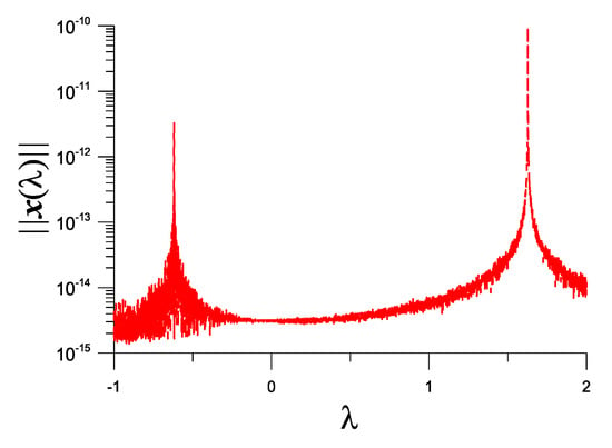
Figure 3. For example 1, showing two peaks in the response curve obtained from the IDM, corresponding to eigenvalues −0.619402940600584 and 1.627440079051887.

Starting from $[a_0,b_0]=[-1,0]$ and under a convergence criterion ${10}^{-15}$, with seven iterations we can obtain $\lambda =-0.6194029406657194$, which is very close to −0.619402940600584 with a difference $4.38\times {10}^{-9}$. On the other hand, the error to satisfy Equation (10) is very small with $\parallel \mathbf{A}\mathbf{x}-\lambda \mathbf{B}\mathbf{x}\parallel =1.93\times {10}^{-15}$, where $\mathbf{x}$ is solved from Equations (32)–(35) with $j_0=3$.

Starting from $[a_0,b_0]=[1,2]$ and with six iterations, we can obtain $\lambda =1.627440079500534$, which is very close to 1.627440079051887 with a difference $1.55\times {10}^{-8}$, and $\parallel \mathbf{A}\mathbf{x}-\lambda \mathbf{B}\mathbf{x}\parallel =1.25\times {10}^{-15}$ is obtained.

Example 2.

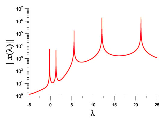
In Equation (10), $\mathbf{A}$ and $\mathbf{B}$ are given in Equation (13). We take $m=5$ and plot $\parallel \mathbf{x}\left(\lambda \right)\parallel$ vs. λ in Figure 4, where five peaks in the response curve happen at five eigenvalues.

Figure 4. For example 2, showing five peaks in the response curve obtained from the IDM, corresponding to five eigenvalues.

Starting from $[a_0,b_0]=[-1,1]$ and under a convergence criterion ${10}^{-12}$, through five iterations $\lambda =-0.1873528931969792$ is obtained. $\parallel \mathbf{A}\mathbf{x}-\lambda \mathbf{B}\mathbf{x}\parallel =4.96\times {10}^{-14}$ is obtained, where $\mathbf{x}$ is solved from Equations (32)–(35) with $j_0=1$.

Starting from $[a_0,b_0]=[1,5]$ and under a convergence criterion ${10}^{-15}$, we can obtain $\lambda =1.313278952662423$ and $\parallel \mathbf{A}\mathbf{x}-\lambda \mathbf{B}\mathbf{x}\parallel =3.77\times {10}^{-14}$ after seven iterations.

With $[a_0,b_0]=[5,10]$ and seven iterations, we can obtain $\lambda =5.537956370847875$ and $\parallel \mathbf{A}\mathbf{x}-\lambda \mathbf{B}\mathbf{x}\parallel =3.19\times {10}^{-15}$.

With $[a_0,b_0]=[10,15]$ and seven iterations, we can obtain $\lambda =12.089692853066820$ and $\parallel \mathbf{A}\mathbf{x}-\lambda \mathbf{B}\mathbf{x}\parallel =2.84\times {10}^{-15}$.

With $[a_0,b_0]=[15,25]$ and seven iterations, we can obtain $\lambda =21.246424716619960$ and $\parallel \mathbf{A}\mathbf{x}-\lambda \mathbf{B}\mathbf{x}\parallel =3.98\times {10}^{-15}$.

By comparing the response curve in Figure 4 with that in Figure 1b, the numerical noise is disappeared by using the IDM in the affine Krylov subspace.

Example 3.

Let $\mathbf{A}=\left[a_{ij}\right]$ and $\mathbf{B}=\left[b_{ij}\right]$, $i,j=1,\dots ,n$. In Equation (10), we take [21]:

$$a_{ii}=\frac{n-i}{100},a_{i,i+1}=\frac{1}{100},i=1,\dots ,n-1,b_{ii}=1,i=81,\dots ,n.$$

(37)

Other elements are all zeros, where we take $n=100$. The eigenvalues are ${\lambda }_j=(j-1)/100$ for $j=1,\dots ,20$.

We take $m=50$ and plot $\parallel \mathbf{x}\left(\lambda \right)\parallel$ vs. $\lambda$ in Figure 5a, where five peaks are obtained by the IDM, which correspond to the first five eigenvalues. Within a finer interval $[a,b]=[0.005,0.015]$ in Figure 5b, one peak appears at a more precise position.

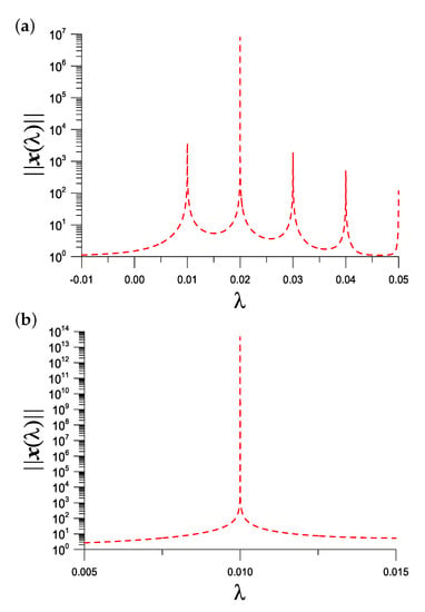
Figure 5. For example 3, (a) showing five picks of $\parallel \mathbf{x}\parallel$ with $m=50$ in the interval [−0.01,0.05], and (b) a pick of $\parallel \mathbf{x}\parallel$ is enlarged in the interval [0.005,0.015], which is a process of zoom-in.

Starting from $[a_0,b_0]=[0.005,0.015]$ and with one iteration under a convergence criterion ${10}^{-15}$, the eigenvalue obtained is very close to 0.01 with an error $2.24\times {10}^{-10}$. $\parallel \mathbf{A}\mathbf{x}-\lambda \mathbf{B}\mathbf{x}\parallel =1.803\times {10}^{-18}$ is obtained, where $\mathbf{x}$ is solved from Equations (32)–(35) with $j_0=99$.

With $[a_0,b_0]=[0.011,0.021]$ and $j_0=99$, after two iterations the eigenvalue obtained is very close to 0.02 with an error $4.47\times {10}^{-10}$. $\parallel \mathbf{A}\mathbf{x}-\lambda \mathbf{B}\mathbf{x}\parallel =2.236\times {10}^{-19}$ is obtained.

For this problem, if we take $m=n$ and $\mathbf{U}={\mathbf{I}}_n$ to compute the eigenvalue in the full space, the computational time is increased. The CPU time spent to construct the response curve is 6.09 s. For the eigenvalue 0.01 the error is the same with $2.24\times {10}^{-10}$, but the CPU time increases to 5.83 s. In contrast, the subspace method spent 1.05 s to construct the response curve, and the CPU time for the eigenvalue 0.01 is 1.05 s. When n is increased to $n=200$, the subspace method with $m=50$ spent 1.05 s to construct the response curve and the CPU time for the eigenvalue 0.01 is 6.53 s; however, by using the full space method with $n=200$ the CPU time is 44.91 s and and CPU time for the eigenvalue 0.01 is 44.67 s. Therefore, the computational efficiency of the m-dimensional affine Krylov subspace method is better than that by using the full space method with dimension n.

To further test the efficiency of the proposed method, we consider the eigenvalue problem of Hilbert matrix [31]. In Equation (10), we take $\mathbf{B}={\mathbf{I}}_n$ and

$$a_{ij}=\frac{1}{i+j-1},i,j=1,\dots ,n.$$

(38)

Due to highly ill-conditioned nature of the Hilbert matrix, it is a quite difficult eigenvalue problem. For this problem, we take $n=100$, $m=30$ and $j_0=50$ to compute the largest eigenvalue, which is given as 2.182696097757424. The affine Krylov subspace method is convergent very fast with six iterations, and the CPU time is 1.52 s. The error of eigen-equation is $\parallel \mathbf{A}\mathbf{x}-\lambda \mathbf{B}\mathbf{x}\parallel =2.005\times {10}^{-13}$. However, finding the largest eigenvalue in the full space with dimension $n=100$, it does not converge within 100 iterations, and the CPU time is increased to 33.12 s. By using the MATLAB, we obtain 2.182696097757423 which is close to that obtained by the Krylov subspace method. However, the MATLAB leads to a large error of Det$(\mathbf{A}\mathbf{x}-\lambda \mathbf{B}\mathbf{x})=6.94680072753434\times {10}^{17}$, which indicates that the characteristic equation for the Hilbert matrix is highly ill-posed. Notice that the smallest eigenvalue is very difficult to be computed, since it is very close to zero. However, we can obtain the smallest eigenvalue $3.1\times {10}^{-19}$ with one iteration and the error $\parallel \mathbf{A}\mathbf{x}-\lambda \mathbf{B}\mathbf{x}\parallel =9.412\times {10}^{-17}$ is obtained. For the eigenvalue problem of the Hilbert matrix, the MATLAB leads to a wrong eigenvalue $-9.693294591063901\times {10}^{-17}$, which is negative and contradicts to the positive eigenvalues of the Hilbert matrix. The eig function in Matlab cannot guarantee to obtain a positive eigenvalue for the positive definite Hilbert matrix. The first 41 eigenvalues are all negative. The first 73 eigenvalues are less than ${10}^{-17}$. So most of these eigenvalues computed by Matlab should be spurious. The MATLAB is effective for general purpose eigenvalue problem with normal matrices, but for the highly ill-conditioned matrices the effectiveness of the MATLAB might be lost.

In addition to the computational efficiency, the Krylov subspace method has several advantages including easy-implementation, the ability to detect all eigenvalues and computing all the corresponding eigenfunctions simultaneously. One can roughly locate the eigenvalues from the peaks in the response curve and then determine precise value by using the IDM. Although for the eigenvalue problem of the highly ill-conditioned Hilbert matrix, the Krylov subspace method is reliable.

6. An Iterative Detection Method for Complex Eigenvalue

Instead linearizing Equation (3) to a linear generalized eigenvalue problem in Equation (10), we directly treat the quadratic eigenvalue problem (3). Now, we consider the detection of complex eigenvalue of the quadratic eigenvalue problem (3). Because $\mathbf{M}$, $\mathbf{C}$ and $\mathbf{K}$ are real matrices, the complex eigenvalue is written by Equation (14). When we take

$$\mathbf{u}=\mathbf{v}+i\mathbf{w},$$

(39)

inserting Equations (14) and (39) into Equation (3) yields

$$\left[\begin{array}{cc}({\lambda }_R^2-{\lambda }_I^2)\mathbf{M}+{\lambda }_R\mathbf{C}+\mathbf{K}& -2{\lambda }_R{\lambda }_I\mathbf{M}-{\lambda }_I\mathbf{C}\\ 2{\lambda }_R{\lambda }_I\mathbf{M}+{\lambda }_I\mathbf{C}& ({\lambda }_R^2-{\lambda }_I^2)\mathbf{M}+{\lambda }_R\mathbf{C}+\mathbf{K}\end{array}\right]\left[\begin{array}{c}\mathbf{v}\\ \mathbf{w}\end{array}\right]=\mathbf{0}.$$

(40)

Letting

$$\mathbf{X}:=\left[\begin{array}{c}\mathbf{v}\\ \mathbf{w}\end{array}\right],\mathbf{D}:=\left[\begin{array}{cc}({\lambda }_R^2-{\lambda }_I^2)\mathbf{M}+{\lambda }_R\mathbf{C}+\mathbf{K}& -2{\lambda }_R{\lambda }_I\mathbf{M}-{\lambda }_I\mathbf{C}\\ 2{\lambda }_R{\lambda }_I\mathbf{M}+{\lambda }_I\mathbf{C}& ({\lambda }_R^2-{\lambda }_I^2)\mathbf{M}+{\lambda }_R\mathbf{C}+\mathbf{K}\end{array}\right],$$

(41)

Equation (40) becomes

$$\mathbf{D}\mathbf{X}=\mathbf{0},$$

(42)

which is an $n=2q$ dimensional homogeneous linear system.

Taking

$$\mathbf{X}={\mathbf{X}}_0+\mathbf{Y},$$

(43)

where ${\mathbf{X}}_0\ne \mathbf{0}$ is a given exciting vector and by Equation (42), we have

$$\mathbf{D}\mathbf{Y}=-\mathbf{D}{\mathbf{X}}_0.$$

(44)

The numerical procedures for determining the complex eigenvalue of the quadratic eigenvalue problem (3) are summarized as follows. (i) Give q, ${\mathbf{X}}_0$, a and b. (ii) For each collocating point $({\lambda }_R,{\lambda }_I)\in [a,b]\times [c,d]$ solving Equation (44) to obtain $\mathbf{X}={\mathbf{X}}_0+\mathbf{Y}$ and taking the optimal $({\lambda }_R,{\lambda }_I)$ to satisfy

$$\underset{({\lambda }_R,{\lambda }_I)\in [a,b]\times [c,d]}{max}\parallel \mathbf{X}({\lambda }_R,{\lambda }_I)\parallel ,$$

(45)

where the size of $[a,b]\times [c,d]$ must be large enough to include at least one complex eigenvalue.

By Equation (45), we gradually reduce the size of the rectangle centered at the previous peak point by renewing the range to a finer one. Give an initial interval $[a_k,b_k]\times [c_k,d_k],k=0$, and we fix the collocating points by ${\lambda }_R\left(i\right)=a_k+i(b_k-a_k)/N_1,i=0,\dots ,N_1$, ${\lambda }_I\left(j\right)=c_k+i(d_k-c_k)/N_2,j=0,\dots ,N_2$ and pick up the maximal point denoted by $({\lambda }_R^k,{\lambda }_I^k)$. Then, a finer rectangle is given by $(a_{k+1},b_{k+1})=({\lambda }_R^k-(b_k-a_k)/N_3,{\lambda }_R^k+(b_k-a_k)/N_3)$, and $(c_{k+1},d_{k+1})=({\lambda }_I^k-(d_k-c_k)/N_3,{\lambda }_I^k+(d_k-c_k)/N_3)$, and in that new rectangle we pick up the new maximum point denoted by $({\lambda }_R^{k+1},{\lambda }_I^{k+1})$. Continuing this process until $\sqrt{{({\lambda }_R^{k+1}-{\lambda }_R^k)}^2+{({\lambda }_I^{k+1}-{\lambda }_I^k)}^2}<\epsilon$, we can obtain the complex eigenvalue with high accuracy. This algorithm is shortened as an iterative detection method (IDM).

When the complex eigenvalue is computed, we can apply the techniques in Equations (32)–(35) with $\mathbf{x}$ replaced by $\mathbf{X}$ and $\mathbf{A}-\lambda \mathbf{B}$ by $\mathbf{D}$ in Equation (42) to compute the complex eigen-mode. The numerical procedures to detect the complex eigenvalue and to compute the complex eigenvector in Equations (14)–(18) for the generalized eigenvalue problem (10) are the same to those in the above.

7. Examples of Quadratic Eigenvalue Problems

7.1. Linearizing Method

For the quadratic eigenvalue problem (3) there are two major methods: Linearization method to a generalized eigenvalue problem as shown by Equation (10) and the decomposition method based on the generalized Bezout method as shown by Equations (4)–(6). In this section, we give two examples of the quadratic eigenvalue problem (3) solved by an iterative detection method in Section 4 for the resultant generalized eigenvalue problem, and developing a direct detection method to Equation (3) for the applications to other three examples.

Example 4.

We consider the structural system (1) with [4]:

$$\mathbf{M}=\left[\begin{array}{ccc}0& 6& 0\\ 0& 6& 0\\ 0& 0& 1\end{array}\right],\mathbf{C}=\left[\begin{array}{ccc}1& -6& 0\\ 2& -7& 0\\ 0& 0& 0\end{array}\right],\mathbf{K}={\mathbf{I}}_3.$$

(46)

There exist four real eigenvalues $\lambda =\{1/3,1/2,1,\infty \}$ and two imaginary eigenvalues i and $-i$.

According to Equations (9) and (10), we can write

$$\mathbf{A}=\left[\begin{array}{cccccc}0& 0& 0& 1& 0& 0\\ 0& 0& 0& 0& 1& 0\\ 0& 0& 0& 0& 0& 1\\ -1& 0& 0& -1& 6& 0\\ 0& -1& 0& -2& 7& 0\\ 0& 0& -1& 0& 0& 0\end{array}\right],\mathbf{B}=\left[\begin{array}{cccccc}1& 0& 0& 0& 0& 0\\ 0& 1& 0& 0& 0& 0\\ 0& 0& 1& 0& 0& 0\\ 0& 0& 0& 0& 6& 0\\ 0& 0& 0& 0& 6& 0\\ 0& 0& 0& 0& 0& 1\end{array}\right].$$

(47)

We take $m=6$ and plot $\parallel \mathbf{x}\left(\lambda \right)\parallel$ vs. $\lambda$ in Figure 6, where three peaks happen at $\lambda =\{1/3,1/2,1\}$. Starting from $[a_0,b_0]=[0,0.4]$ and under a convergence criterion ${10}^{-15}$, through six iterations $\lambda =0.3333333333333386$ is obtained with $\parallel \mathbf{A}\mathbf{x}-\lambda \mathbf{B}\mathbf{x}\parallel =1.82\times {10}^{-15}$, where $\mathbf{x}$ is solved from Equations (32)–(35) with $j_0=1$. Starting from $[a_0,b_0]=[0.4,0.6]$ and after one iteration, we can obtain $\lambda =0.5$ and $\parallel \mathbf{A}\mathbf{x}-\lambda \mathbf{B}\mathbf{x}\parallel =1.01\times {10}^{-15}$ is obtained. Starting from $[a_0,b_0]=[0.7,1.5]$ and after two iterations, we can obtain $\lambda =1$ and $\parallel \mathbf{A}\mathbf{x}-\lambda \mathbf{B}\mathbf{x}\parallel =1.85\times {10}^{-17}$, where $\mathbf{x}$ is solved from Equations (32)–(35) with $j_0=2$.

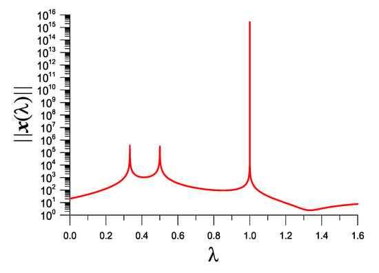
Figure 6. For example 4, showing three picks of $\parallel \mathbf{x}\parallel$ in the response curve in the interval [0,1.6].

By Equation (47), we cannot recover $\lambda =\infty$. To remedy this defect, we notice that Equation (3) can also be expressed by Equation (10) with

$$\mathbf{A}:=\left[\begin{array}{cc}-\mathbf{K}& {\mathbf{0}}_q\\ {\mathbf{0}}_q& -{\mathbf{I}}_q\end{array}\right],\mathbf{B}:=\left[\begin{array}{cc}\mathbf{C}& \mathbf{M}\\ -{\mathbf{I}}_q& {\mathbf{0}}_q\end{array}\right].$$

(48)

By Equations (10) and (48), we can take

$$\mathbf{A}=-{\mathbf{I}}_6,\mathbf{B}=\left[\begin{array}{cccccc}1& -6& 0& 0& 6& 0\\ 2& -7& 0& 0& 6& 0\\ 0& 0& 0& 0& 0& 1\\ -1& 0& 0& 0& 0& 0\\ 0& -1& 0& 0& 0& 0\\ 0& 0& -1& 0& 0& 0\end{array}\right].$$

(49)

Let $\mu =-1/\lambda$. We can set up a new eigenvalue problem:

$$\mathbf{B}\mathbf{x}=\mu \mathbf{x}.$$

(50)

We take $m=6$ and plot $\parallel \mathbf{x}\left(\mu \right)\parallel$ vs. $\mu$ in Figure 7a, where we can observe four peaks happened at $\mu =\{-3,-2,-1,0\}$, by which we can recover $\lambda =\{1/3,1/2,1,\infty \}$ by using $\lambda =-1/\mu$.

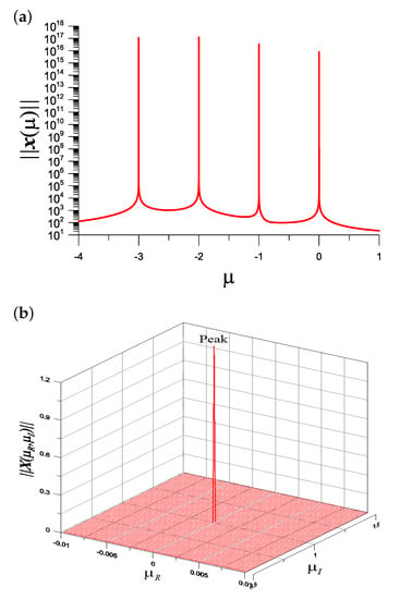
Figure 7. For example 4, (a) showing four picks of $\parallel \mathbf{x}\parallel$ in the response curve in the interval [−4,1], and (b) a pick of $\parallel \mathbf{x}\parallel$ over the plane is enlarged in the interval $[-0.01,0.01]\times [0.5,1.5]$.

Starting from $[a_0,b_0]=[-3.5,-2.5]$ and under a convergence criterion ${10}^{-15}$, after one iteration $\mu =-3$ is obtained, and $\parallel \mathbf{B}\mathbf{x}-\mu \mathbf{x}\parallel =1.11\times {10}^{-15}$, where $\mathbf{x}$ is solved from Equations (32)–(35) with $j_0=1$. Starting from $[a_0,b_0]=[-2.5,-1.5]$ and after one iteration, we can obtain $\mu =-2$ and $\parallel \mathbf{B}\mathbf{x}-\mu \mathbf{x}\parallel =2.04\times {10}^{-15}$. Starting from $[a_0,b_0]=[-1.5,-0.5]$ and after one iteration, we can obtain $\mu =-1$ and $\parallel \mathbf{B}\mathbf{x}-\mu \mathbf{x}\parallel =1.07\times {10}^{-14}$ is obtained, where $\mathbf{x}$ is solved from Equations (32)–(35) with $j_0=2$. Starting from $[a_0,b_0]=[-0.5,0.5]$ and after one iteration, we can obtain $\mu =0$.

We employ the IDM in Section 6 to locate the complex eigenvalue as shown in Figure 7b. We find that with the initial guess $[a_0,b_0]\times [c_0,d_0]=[-0.01,0.01]\times [0.5,1.5]$, we can find ${\mu }_R=0$ and ${\mu }_I=1$ with one iteration.

By the same token, when we locate the complex eigenvalue of Equation (21) with the initial guess $[a_0,b_0]\times [c_0,d_0]=[1,2]\times [0.5,1]$, we can find ${\lambda }_R=3/2$ and ${\lambda }_I=0.8660254037844387$ within ten iterations. Upon comparing to the exact one in Equation (22) the error is $1.11\times {10}^{-16}$, which is very accurate, and the IDM is convergent very fast.

In the structural dynamics the coefficient matrices $\mathbf{M}$, $\mathbf{C}$ and $\mathbf{K}$ are symmetric; moreover, $\mathbf{M}$ and $\mathbf{K}$ are positive definite matrices. This example with a non-positive definite matrix $\mathbf{M}$ and a non-symmetric matrix $\mathbf{C}$ is borrowed from the literature [4]. This eigenvalue problem has an infinity eigenvalue.

Example 5.

We consider a free vibration problem of an MK structural system with [1]:

$$\mathbf{M}=m_0\mathbf{B}=m_0\left[\begin{array}{ccc}1& 0& 0\\ 0& 1& 0\\ 0& 0& 2\end{array}\right],\mathbf{K}=k_0\mathbf{A}=k_0\left[\begin{array}{ccc}2& -1& 0\\ -1& 3& -2\\ 0& -2& 2\end{array}\right].$$

(51)

By inserting $\mathbf{y}=\mathbf{x}{e}^{i\omega t}$ into Equation (1) with $\mathbf{C}=\mathbf{0}$, we can derive

$$\mathbf{K}\mathbf{x}={\omega }^2\mathbf{M}\mathbf{x}.$$

(52)

Let $\lambda =m_0{\omega }^2/k_0$ for $\mathbf{A}\mathbf{x}=\lambda \mathbf{B}\mathbf{x}$. We take $m=3$ and plot $\parallel \mathbf{x}\left(\lambda \right)\parallel$ vs. $\lambda$ in Figure 8, where we can observe three peaks, whose precise values are 0.1391941468883, 1.745898311614913 and 4.114907541476740, respectively. Those values coincide to the roots obtained from the characteristic equation Det$(\mathbf{A}-\lambda \mathbf{B})=0$, that is,

$${\lambda }^3-6{\lambda }^2+8\lambda -1=0.$$

(53)

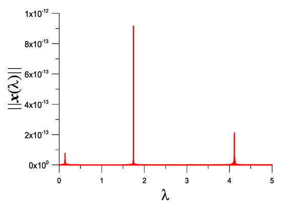
Figure 8. For example 5, showing three picks of $\parallel \mathbf{x}\parallel$ in the response curve in the interval [0,5].

The corresponding natural frequencies are $0.3730873180480677\sqrt{k_0/m_0}$, $1.321324453574864\sqrt{k_0/m_0}$ and $2.028523488026880\sqrt{k_0/m_0}$, respectively.

Starting from $[a_0,b_0]=[0,0.5]$ and under a convergence criterion ${10}^{-10}$, with four iterations $\parallel \mathbf{A}\mathbf{x}-\lambda \mathbf{B}\mathbf{x}\parallel =1.79\times {10}^{-15}$ is obtained, where $\mathbf{x}$ is solved from Equations (32)–(35) with $j_0=1$. Starting from $[a_0,b_0]=[1,2]$ and with five iterations, we can obtain $\parallel \mathbf{A}\mathbf{x}-\lambda \mathbf{B}\mathbf{x}\parallel =7.63\times {10}^{-11}$. Starting from $[a_0,b_0]=[4,5]$ and with four iterations, we can obtain $\parallel \mathbf{A}\mathbf{x}-\lambda \mathbf{B}\mathbf{x}\parallel =1.44\times {10}^{-13}$.

The corresponding eigen-modes are given as follows:

$$\begin{array}{c}{\mathbf{x}}^{\left(1\right)}=\left[\begin{array}{c}1\\ 1.860805853111704\\ 2.161702138043240\end{array}\right],{\mathbf{x}}^{\left(2\right)}=\left[\begin{array}{c}1\\ 0.2541016883850868\\ -0.3406653217873807\end{array}\right],\hfill \\ {\mathbf{x}}^{\left(3\right)}=\left[\begin{array}{c}1\\ -2.114907541476740\\ 0.6789631837592252\end{array}\right].\hfill \end{array}$$

(54)

We extend the results to a ten-degree system with $m_1=\dots =m_9=m_0$, $m_{10}=2m_0$, $k_1=\dots =k_9=k_0$ and $k_{10}=2k_0$. The response curve of $\parallel \mathbf{x}\left(\lambda \right)\parallel$ vs. $\lambda$ is plotted Figure 9, where we can observe ten peaks. The minimal frequency is $0.1371265436475375\sqrt{k_0/m_0}$ and the maximal frequency is $2.058147747545097\sqrt{k_0/m_0}$.

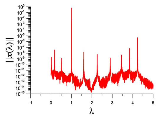
Figure 9. For example 5 with ten-degree, showing ten picks of $\parallel \mathbf{x}\parallel$ in the response curve in the interval [0,5].

As a practical application, we consider a five-story shear building with [32]

$$\begin{array}{c}\mathbf{M}=\left[\begin{array}{ccccc}140& 0& 0& 0& 0\\ 0& 120& 0& 0& 0\\ 0& 0& 120& 0& 0\\ 0& 0& 0& 120& 0\\ 0& 0& 0& 0& 100\end{array}\right]\mathrm{kip/g},\hfill \\ \mathbf{K}=\left[\begin{array}{ccccc}800& -400& 0& 0& 0\\ -400& 600& -200& 0& 0\\ 0& -200& 400& -200& 0\\ 0& 0& -200& 300& -100\\ 0& 0& 0& -100& 100\end{array}\right]\mathrm{kip/in}.\hfill \end{array}$$

(55)

We take $m=5$ and plot $\parallel \mathbf{x}\left(\lambda \right)\parallel$ vs. $\lambda$ in Figure 10a, where we can observe five peaks. Starting from $[a_0,b_0]=[0,1]$ and under a convergence criterion ${10}^{-15}$, with six iterations ${\omega }^2=0.2039991612696613$ is obtained and $\parallel \mathbf{K}\mathbf{x}-{\omega }^2\mathbf{M}\mathbf{x}\parallel =2.85\times {10}^{-13}$ is obtained, where $\mathbf{x}$ is solved from Equations (32)–(35) with $j_0=1$ with the first mode being shown in Figure 10b at the first column.

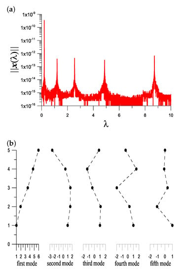
Figure 10. For a five-degree MK system, (a) showing five picks of $\parallel \mathbf{x}\parallel$ in the response curve in the interval [0,10], and (b) displaying the five vibration modes.

Starting from $[a_0,b_0]=[1,2]$ and with seven iterations ${\omega }^2=1.195924448669029$ is obtained and $\parallel \mathbf{K}\mathbf{x}-{\omega }^2\mathbf{M}\mathbf{x}\parallel =2.37\times {10}^{-13}$ is obtained, with the second mode being shown in Figure 10b at the second column.

Starting from $[a_0,b_0]=[2,3]$ and with six iterations ${\omega }^2=2.55144529001161$ is obtained and $\parallel \mathbf{K}\mathbf{x}-{\omega }^2\mathbf{M}\mathbf{x}\parallel =1.43\times {10}^{-13}$ is obtained, with the third mode being shown in Figure 10b at the third column.

Starting from $[a_0,b_0]=[4,5]$ and with six iterations ${\omega }^2=4.870842516791811$ is obtained and $\parallel \mathbf{K}\mathbf{x}-{\omega }^2\mathbf{M}\mathbf{x}\parallel =2.33\times {10}^{-12}$ is obtained, with the fourth mode being shown in Figure 10b at the fourth column.

Starting from $[a_0,b_0]=[8,9]$ and under a convergence criterion ${10}^{-15}$, with six iterations ${\omega }^2=8.725407630876937$ is obtained, and $\parallel \mathbf{K}\mathbf{x}-{\omega }^2\mathbf{M}\mathbf{x}\parallel =1.78\times {10}^{-11}$ is obtained, where $\mathbf{x}$ is solved from Equations (32)–(35) with $j_0=1$, and the fifth mode is shown in Figure 10b at the fifth column. We have compared to the exact solution ${\omega }^2=8.725407630876935$ solved from the characteristic equation Det$(\mathbf{K}-{\omega }^2\mathbf{M})=0$ with an error $3.05\times {10}^{-8}$, which is given by

$$\begin{array}{ccc}\hfill & & \left|\begin{array}{ccccc}800-140{\omega }^2& -400& 0& 0& 0\\ -400& 600-120{\omega }^2& -200& 0& 0\\ 0& -200& 400-120{\omega }^2& -200& 0\\ 0& 0& -200& 300-120{\omega }^2& -100\\ 0& 0& 0& -100& 100-100{\omega }^2\end{array}\right|\hfill \\ & & =[(800-140{\omega }^2)(600-120{\omega }^2)-160000][(400-120{\omega }^2)(300-120{\omega }^2)(100-100{\omega }^2)\hfill \\ & & -10000(400-120{\omega }^2)-40000(100-100{\omega }^2)]\hfill \\ & & -40000(800-140{\omega }^2)[(300-120{\omega }^2)(100-100{\omega }^2)-10000]=0.\hfill \end{array}$$

(56)

The result ${\omega }^2=8.8746$ presented in [32] has an error 0.1492, which is much more larger than $3.05\times {10}^{-8}$. The advantage of the presented method is convergent fast and very accurate. The errors of the characteristic equation from the first to fifth eigenvalues are, respectively, Det$(\mathbf{K}-{\omega }^2\mathbf{M})=-1.83\times {10}^{-4}$, $-3.66\times {10}^{-4}$, $-1.22\times {10}^{-4}$, $-3.78\times {10}^{-3}$ and $-3.52\times {10}^{-2}$.

The fundamental modes and frequencies obtained at here are convergent faster and more accurate than the Stodola iteration method as described in [32]. We have checked the accuracy to satisfy the characteristic equation Det$(\mathbf{K}-{\omega }^2\mathbf{M})=0$, which is about in the orders ${10}^{-4}$ to ${10}^{-2}$ by the presented method. But with the Stodola method its accuracy is poor with very large error in the order ${10}^{12}$ for the fifth eigenvalue to satisfy the characteristic equation. One reason to cause the large error is that even with a small error of ${\omega }^2$ obtained by the Stodola method, it is amplified by the product of large coefficients in $\mathbf{M}$ and $\mathbf{K}$ with the amount $5.76\times {10}^{12}$, which is estimated by the product of the diagonal elements of $\mathbf{K}$.

7.2. Direct Detection Method

Example 6.

Let $\mu =1/\lambda$, Equation (3) can be written as

$$(\mathbf{M}+\mu \mathbf{C}+{\mu }^2\mathbf{K})\mathbf{u}=0.$$

(57)

By letting

$$\mathbf{D}:=\mathbf{M}+\mu \mathbf{C}+{\mu }^2\mathbf{K},\mathbf{u}={\mathbf{u}}_0+\mathbf{v},$$

(58)

we come to a nonhomogeneous linear system:

$$\mathbf{D}\mathbf{v}=-\mathbf{D}{\mathbf{u}}_0,$$

(59)

where ${\mathbf{u}}_0$ is a nonzero constant exciting vector.

We apply the IDM in Section 4 to directly detect the real eigenvalues of example 4, and plot $\parallel \mathbf{u}\left(\mu \right)\parallel$ vs. $\mu$ in Figure 11, where four peaks are happened at $\mu =\{0,1,2,3\}$, by which we can recover $\lambda =\{1/3,1/2,1,\infty \}$ by using $\lambda =1/\mu$.

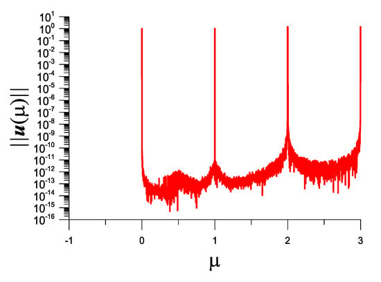
Figure 11. For example 4 solved as a quadratic eigenvalue problem, showing four picks of $\parallel \mathbf{u}\parallel$ in the response curve in the interval [0,3].

Starting from $[a_0,b_0]=[-0.5,0.5]$ and under a convergence criterion ${10}^{-15}$, with six iterations $\mu =-6.56\times {10}^{-4}$ is obtained. Starting from $[a_0,b_0]=[0.5,1.5]$ and with six iterations, we can obtain $\mu =1.000656781471890$ and $\parallel \mathbf{D}\mathbf{u}\parallel =4.63\times {10}^{-4}$. Starting from $[a_0,b_0]=[1.5,2.5]$ and after one iteration, we can obtain $\mu =2$ and $\parallel \mathbf{D}\mathbf{u}\parallel =0$. Starting from $[a_0,b_0]=[2.5,4.5]$ and after two iterations, we can obtain $\mu =3$ and $\parallel \mathbf{D}\mathbf{u}\parallel =2.48\times {10}^{-16}$.

The eigen-modes corresponding to $\lambda =\{1/3,1/2,1\}$ are given as follows:

$${\mathbf{u}}^{\left(1\right)}=\left[\begin{array}{c}1\\ 1\\ 0\end{array}\right],{\mathbf{u}}^{\left(2\right)}=\left[\begin{array}{c}1\\ 1\\ 0\end{array}\right],{\mathbf{u}}^{\left(3\right)}=\left[\begin{array}{c}1.805\times {10}^{-3}\\ 1\\ 0\end{array}\right].$$

(60)

Example 7.

We consider [12,33]:

$$\mathbf{M}=\left[\begin{array}{ccc}17.6& 1.28& 2.89\\ 1.28& 0.824& 0.413\\ 2.89& 0.413& 0.725\end{array}\right],\mathbf{C}=\left[\begin{array}{ccc}7.66& 2.45& 2.1\\ 0.23& 1.04& 0.223\\ 0.6& 0.756& 0.658\end{array}\right],\mathbf{K}=\left[\begin{array}{ccc}121& 18.9& 15.9\\ 0& 2.7& 0.145\\ 11.9& 3.64& 15.5\end{array}\right].$$

(61)

There exist three pairs of complex eigenvalues.

Beginning with $[a_0,b_0]\times [c_0,d_0]=[-1,-0.5]\times [8.4,8.5]$, $[a_0,b_0]\times [c_0,d_0]=[0,0.2]\times [2,3]$, and $[a_0,b_0]\times [c_0,d_0]=[-1,-0.5]\times [1,2]$, respectively, and under a convergence criterion ${10}^{-15}$, the IDM with 11 iterations converges to the following eigenvalues:

$$\left[\begin{array}{c}{\lambda }_1\\ {\lambda }_2\\ {\lambda }_3\end{array}\right]=\left[\begin{array}{c}-0.8848302276193034\pm i8.441512059499651\\ 0.09472173815159692\pm i2.52287655639731\\ 0.9179981428161037\pm i1.760584228706396\end{array}\right],$$

(62)

whose corresponding complex eigen-modes are with the errors $\parallel \mathbf{D}\mathbf{X}\parallel =7.45\times {10}^{-14}$, $\parallel \mathbf{D}\mathbf{X}\parallel =3.02\times {10}^{-14}$ and $\parallel \mathbf{D}\mathbf{X}\parallel =7.43\times {10}^{-15}$, respectively. The accuracy of the eigevalues and eigen-modes is in the order of ${10}^{-14}$ or ${10}^{-15}$.

Example 8.

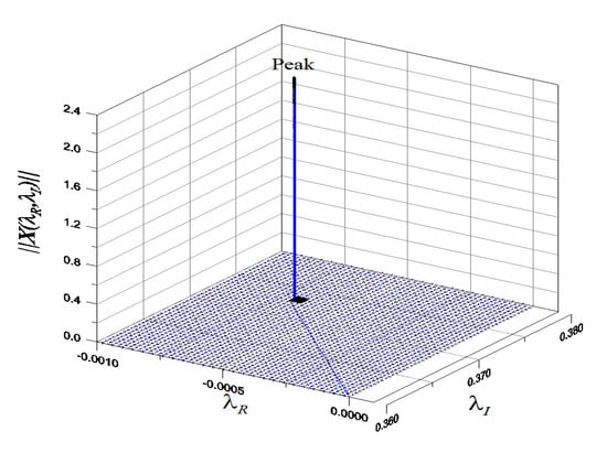
We extend example 5 to a q-degree MCK system with $m_1=\dots =m_{q-1}=1$, $m_q=2$, $c_1=\dots =c_{q-1}=0.01$, $c_q=0.02$, and $k_1=\dots =k_{q-1}=1$ and $k_q=2$. With $q=3$, we employ the IDM in Section 6 to locate the complex eigenvalue, and over the plane there exists one peak in Figure 12. We find that with the initial guess $[a_0,b_0]\times [c_0,d_0]=[-0.001,0]\times [0.36,0.38]$ and $j_0=4$, we can find ${\lambda }_R=-0.0006959802368$ and ${\lambda }_I=0.3730861090816$ with six iterations. The corresponding complex eigen-mode is given by

$$\mathbf{u}=\mathbf{v}+i\mathbf{w}=\left[\begin{array}{c}-0.01700169666735284\\ -0.03163685511252461\\ -0.03.675260035588075\end{array}\right]+i\left[\begin{array}{c}1\\ 1.860806270952949\\ 2.161703124485385\end{array}\right],$$

(63)

whose error $\parallel \mathbf{D}\mathbf{X}\parallel =2.67\times {10}^{-6}$ is obtained.

Figure 12. For example 7, showing a pick of $\parallel \mathbf{u}\parallel$ in the response surface for complex eigenvalues.

For $q=5$, we find that with the initial guess $[a_0,b_0]\times [c_0,d_0]=[-0.1,0]\times [0.1,0.5]$ and $j_0=5$, we can find ${\lambda }_R=-0.0003059040256$ and ${\lambda }_I=0.24710529040384$ with seven iterations, and the error $\parallel \mathbf{D}\mathbf{X}\parallel =2.08\times {10}^{-5}$ is obtained.

In Figure 13, with $j_0=3$ we plot the maximal and minimal frequencies with respect to q, which can be seen that the maximal frequencies are insensitive to the dimension q of the MCK system.

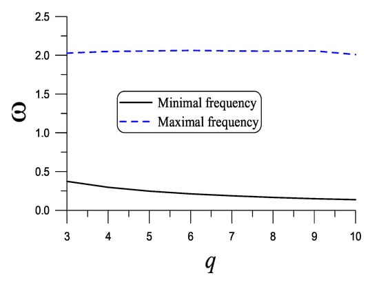
Figure 13. For example 7 with different dimension, showing maximal and minimal frequencies.

Remark 1.

The presented IDM is easily extended to nonlinear eigenvalue problem [34]. For example, we change Equation (3) to

$$({\lambda }^2\mathbf{M}+\sqrt{\lambda }\mathbf{C}+\mathbf{K})\mathbf{u}=0,$$

(64)

where $\mathbf{M}$, $\mathbf{C}$ and $\mathbf{K}$ are given by Equation (46). Equation (64) cannot be linearized to a linear one as that in Equation (10).

It is interesting that the original real eigenvalues $\mu =\{0,1,2,3\}=1/\lambda$ are changed to three as shown in Figure 14, where we can observe three peaks. Starting from $[a_0,b_0]=[0.8,1.1]$ and with six iterations, we can obtain $\mu =1.001315771923528$ and $\parallel \mathbf{D}\mathbf{u}\parallel =4.62\times {10}^{-4}$. Starting from $[a_0,b_0]=[1.1,1.5]$ and with six iterations, we can obtain $\mu =1.346624934599962$ and $\parallel \mathbf{D}\mathbf{u}\parallel =2.58\times {10}^{-9}$.

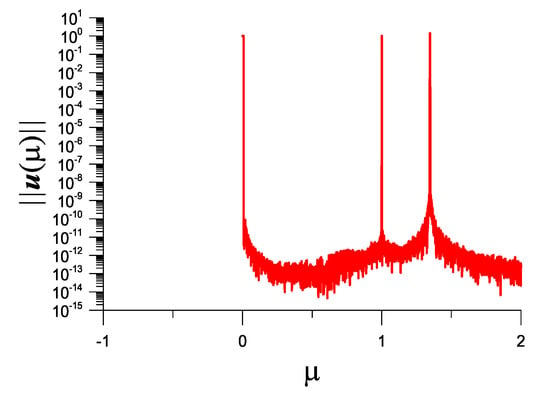
Figure 14. For a nonlinear perturbation of example 4, showing three picks of $\parallel \mathbf{u}\parallel$ in the response curve in the interval [0,2].

8. Conclusions

This paper was concerned with the fast iterative solutions of generalized and quadratic eigenvalue problems. Since the vector eigen-equation is a homogeneous linear system, the eigenvector is either a zero vector when the eigen-parameter is not an eigenvalue, or an unknown vector when the eigen-parameter is an eigenvalue. Based on the original eigen-equation, we cannot construct the response curve, which is the magnitude of the eigenvector with respect to the eigen-parameter. We transformed the eigenvector to a new vector including a nonzero exciting vector, which by inserting into the original eigen-equation yields a nonhomogeneous linear system for the new vector. By varying the eigen-parameter in a desired interval, we can construct the response curve. This is a new idea of the so-called excitation method (EM). Then, by maximizing the magnitude of the eigenvector solved from the nonhomogeneous linear system, we can quickly detect the location of the eigenvalue, which is a peak in the response curve. To precisely obtain the eigenvalue, we developed an iterative detection method (IDM) by sequentially reducing the size of the searching interval. For reducing the computational cost of the generalized eigenvalue problem, we derived the nonhomogeneous linear system in a lower m-dimensional affine Krylov subspace. If m is large enough and $m<n$, the presented method can find all eigenvalues very effectively. Then, we reduced the eigen-equation with one dimension less to a nonhomogeneous linear system to determine the eigenvector with high accuracy.

In summary, the key outcomes are pointed out here.

• We transformed the eigenvector to a new vector including a nonzero exciting vector, which by inserting into the original eigen-equation yields a nonhomogeneous linear system for the new vector.
• By varying the eigen-parameter in a desired interval, we can construct the response curve.
• By maximizing the magnitude of the eigenvector solved from the nonhomogeneous linear system, we can quickly detect the location of the eigenvalue, which is a peak in the response curve.
• To precisely obtain the eigenvalue, we developed an iterative detection method (IDM) by sequentially zoom-in.
• From the peaks in the response curve one can roughly locate the eigenvalues and then determine precise value by using the IDM.
• By using the EM and IDM, we have solved the quadratic eigenvalue problem for the application to the free vibrations of multi-degree mechanical systems.
• For the complex eigenvalue we developed the IDM in the eigen-parameter plane of real and imaginary parts of complex eigenvalue. Very accurate eigenvalue and eigen-mode can be obtained merely through a few iterations.

References

- Meirovitch, L. Elements of Vibrational Analysis, 2nd ed.; McGraw-Hill: New York, NY, USA, 1986. [Google Scholar]
- Smith, H.A.; Singh, R.K.; Sorensen, D.C. Formulation and solution of the non-linear, damped eigenvalue problem for skeletal systems. Int. J. Numer. Meth. Engng. 1995, 38, 3071–3085. [Google Scholar] [CrossRef]
- Osinski, Z. (Ed.) Damping of Vibrations; A.A. Balkema: Rotterdam, The Netherlands, 1998. [Google Scholar]
- Tisseur, F.; Meerbergen, K. The quadratic eigenvalue problem. SIAM Rev. 2001, 43, 235–286. [Google Scholar] [CrossRef]
- Cakar, O. Mass and stiffness modifications without changing any specified natural frequency of a structure. J. Vib. Contr. 2011, 17, 769–776. [Google Scholar] [CrossRef]
- Gao, W. Natural frequency and mode shape analysis of structures with uncertainty. Mech. Sys. Sig. Process 2007, 21, 24–39. [Google Scholar] [CrossRef]
- Gantmacher, F.R. The Theory of Matrices 1; Chelsea: New York, NY, USA, 1959. [Google Scholar]
- Kublanovskaya, V.N. On an approach to the solution of the generalized latent value problem for λ-matrices. SIAM J. Numer. Anal. 1970, 7, 532–537. [Google Scholar] [CrossRef]
- Ruhe, A. Algorithms for the nonlinear eigenvalue problem. SIAM J. Numer. Anal. 1973, 10, 674–689. [Google Scholar] [CrossRef]
- Dennis, J.E., Jr.; Traub, J.F.; Weber, R.P. The algebraic theory of matrix polynomials. SIAM J. Numer. Anal. 1976, 13, 831–845. [Google Scholar] [CrossRef][Green Version]
- Davis, G.J. Numerical solution of a quadratic matrix equation. SIAM J. Sci. Stat. Comput. 1981, 2, 164–175. [Google Scholar] [CrossRef]
- Higham, N.J.; Kim, H. Solving a quadratic matrix equation by Newton’s method with exact line searches. SIAM J. Matrix Anal. Appl. 2001, 23, 303–316. [Google Scholar] [CrossRef]
- Higham, N.J.; Kim, H. Numerical analysis of a quadratic matrix equation. IMA J. Numer. Anal. 2000, 20, 499–519. [Google Scholar] [CrossRef]
- Bai, Z.; Su, Y. SOAR: A second-order Arnoldi method for the solution of the quadratic eigenvalue problem. SIAM J. Matrix Anal. Appl. 2005, 26, 640–659. [Google Scholar] [CrossRef]
- Qian, J.; Lin, W.-W. A numerical method for quadratic eigenvalue problems of gyroscopic systems. J. Sound Vib. 2007, 306, 284–296. [Google Scholar] [CrossRef]
- Meerbergen, K. The quadratic Arnoldi method for the solution of the quadratic eigenvalue problem. SIAM J. Matrix Anal. Appl. 2008, 30, 1463–1482. [Google Scholar] [CrossRef]
- Hammarling, S.; Munro, C.J.; Tisseur, F. An algorithm for the complete solution of quadratic eigenvalue problems. ACM Trans. Math. Softw. 2013, 39, 18. [Google Scholar] [CrossRef]
- Guo, C.-H. Numerical solution of a quadratic eigenvalue problem. Linear Algebra Appl. 2004, 385, 391–406. [Google Scholar] [CrossRef][Green Version]
- Chen, C.; Ma, C. An accelerated cyclic-reduction-based solvent method for solving quadratic eigenvalue problem of gyroscopic systems. Comput. Math. Appl. 2019, 77, 2585–2595. [Google Scholar] [CrossRef]
- Golub, G.H.; van Loan, C.F. Matrix Computations; The John Hopkins University Press: Baltimore, MD, USA, 2012. [Google Scholar]
- Sakurai, T.; Sugiura, H. A projection method for generalized eigenvalue problems using numerical integration. J. Comput. Appl. Math. 2003, 159, 119–128. [Google Scholar] [CrossRef]
- Saad, Y. Variations on Arnoldi’s method for computing eigenelements of large unsymmetric matrices. Linear Algebra Its Appl. 1980, 34, 269–295. [Google Scholar] [CrossRef]
- Saad, Y. Chebyshev acceleration techniques for solving nonsymmetric eigenvalue problems. Math. Comput. 1984, 42, 567–588. [Google Scholar] [CrossRef]
- Arnoldi, W.E. The principle of minimized iterations in the solution of the matrix eigenvalue problem. Quart. Appl. Math. 1951, 9, 17–29. [Google Scholar] [CrossRef]
- Saad, Y. Numerical solution of large nonsymmetric eigenvalue problems. Comput. Phys. Commun. 1989, 53, 71–90. [Google Scholar] [CrossRef][Green Version]
- Morgan, R.B. On restarting the Arnoldi method for large nonsymmetric eigenvalue problems. Math. Comput. 1996, 65, 1213–1230. [Google Scholar] [CrossRef]
- Parlett, B.N.; Taylor, D.R.; Liu, Z.A. A look-ahead Lanczos algorithm for unsymmetric matrices. Math. Comput. 1985, 44, 105–124. [Google Scholar]
- Nour-Omid, B.; Parlett, B.N.; Taylor, R.L. Lanczos versus subspace iteration for solution of eigenvalue problems. Int. J. Num. Meth. Eng. 1983, 19, 859–871. [Google Scholar] [CrossRef]
- Liu, C.-S. A doubly optimized solution of linear equations system expressed in an affine Krylov subspace. J. Comput. Appl. Math. 2014, 260, 375–394. [Google Scholar] [CrossRef]
- Saad, Y. Iterative Methods for Sparse Linear Systems, 2nd ed.; SIAM: Philadelphia, PA, USA, 2003. [Google Scholar]
- Fettis, H.E.; Caslin, J.C. Eigenvalues and eigenvectors of Hilbert matrices of order 3 through 10. Math. Comput. 1967, 21, 431–441. [Google Scholar] [CrossRef][Green Version]
- Berg, G.V. Elements of Structural Dynamics; Prentice-Hall: Hoboken, NJ, USA, 1988. [Google Scholar]
- Lancaster, P. Lambda-Matrices and Vibrating Systems; Pergamon Press: Oxford, UK, 1966. [Google Scholar]
- Chiappinelli, R. What do you mean by “nonlinear eigenvalue problems”? Axioms 2018, 7, 39. [Google Scholar] [CrossRef]
Publisher’s Note: MDPI stays neutral with regard to jurisdictional claims in published maps and institutional affiliations. |
© 2022 by the authors. Licensee MDPI, Basel, Switzerland. This article is an open access article distributed under the terms and conditions of the Creative Commons Attribution (CC BY) license (https://creativecommons.org/licenses/by/4.0/).