Heterogeneous Graph Neural Network with Local and Global Message Passing for AC-Optimal Power Flow Solutions

Abstract

The AC Optimal Power Flow (AC-OPF) problem remains a major computational bottleneck for real-time power system operation. Conventional solvers are accurate but time-consuming, while Graph Neural Networks (GNNs) offer faster approximations yet struggle to capture long-range dependencies and handle topological variations. To address these limitations, we propose a Heterogeneous Graph Transformer with bus-centric Local–Global Message Passing (LG-HGNN). The model performs type-specific local message passing over heterogeneous power graphs and applies a global Transformer only on bus nodes to capture system-wide correlations efficiently. Effective-resistance positional encodings and resistance-biased attention enhance electrical awareness, whereas bounded decoders and physics-informed regularization preserve operational feasibility. Experiments on IEEE 14-, 30-, and 118-bus systems show that LG-HGNN achieves near-optimal results within a few percent of the AC-OPF optimum and generalizes to thousands of unseen N-1 contingency topologies without retraining. Compared with interior-point solvers, it attains up to $190\times$ speedup before power-flow correction and over $10\times$ afterward on GOC 2000-bus systems, providing a scalable and physically consistent surrogate for real-time AC-OPF.

1. Introduction

The AC-Optimal Power Flow (AC-OPF) problem represents a cornerstone of power system operations, determining optimal generator dispatch strategies while respecting complex physical and engineering constraints [1]. Despite its fundamental importance across applications such as unit commitment and transmission expansion planning [2], AC-OPF remains computationally formidable for large-scale grids due to its inherent non-convexity and nonlinearity. Existing commercial solvers cannot guarantee globally optimal solutions for large networks within operationally acceptable timeframes [1]. This challenge becomes even more critical as system operators typically solve AC-OPF every 5–15 min [2], and the rapid variability introduced by distributed energy resources (DERs) demands faster and more reliable solution capabilities [3,4].

Although contemporary solvers such as IPOPT have benefited from GPU acceleration and condensed-space algorithms [5], they still fall short of meeting near-real-time requirements and exhibit poor scalability for large transmission systems [6]. Consequently, system operators often rely on mathematical relaxations [7,8] or simplified approximations such as DC-OPF [9]. These methods reduce computational burden but invariably produce sub-optimal and often AC-infeasible solutions [10]. Even small improvements in AC-OPF accuracy may translate into substantial economic and environmental benefits, with estimates suggesting that a 5% improvement in OPF efficiency could save billions of dollars annually [1].

A wide range of methodologies has been proposed to mitigate the computational difficulty of AC-OPF. Classical optimization-based solvers (e.g., Newton and interior-point methods) offer high accuracy but scale poorly and require repeated nonlinear equation solves [11,12]. Heuristic algorithms such as PSO, GA, and ACO [13,14,15] address nonconvexity but incur heavy computational costs and inconsistent convergence. More recently, data-driven models—including fully connected neural networks and deep learning surrogates—have been studied to accelerate OPF computation [16,17,18]. However, non-graph models struggle to generalize across topological variations and often violate AC constraints [2]. Graph Neural Networks (GNNs) alleviate this by explicitly encoding network structure [19,20], yet most existing GNN-based OPF solvers rely on homogeneous graphs and purely local message passing, limiting their ability to capture global electrical dependencies and adapt to N-1 contingency scenarios [21,22].

Graph Neural Networks have therefore received growing interest for AC-OPF due to their natural alignment with power network topologies [19,23]. Nevertheless, existing GNN-based approaches face several fundamental challenges [20,21]: (i) purely local message passing fails to capture long-range dependencies such as global voltage-phase coupling, requiring deep GNN stacks that introduce training instability and over-smoothing; (ii) most architectures rely on homogeneous graph representations, treating buses, generators, shunts, and loads as identical nodes, thereby ignoring inherent physical heterogeneity [24,25]; (iii) recent heterogeneous models [22] still require very deep propagation layers (e.g., 60 layers) for large networks, limiting computational efficiency; (iv) current GNN solvers exhibit limited adaptability to topological variations, often requiring costly retraining for each N-1 contingency case.

To address these challenges, we propose a Heterogeneous Graph Transformer with Local–Global Message Passing (LG-HGNN). Our key contributions are summarized as follows:

• Bus-centric heterogeneous Transformer architecture. We develop a heterogeneous GNN combining local, edge-aware message passing with a bus-centric global Transformer. Global attention is applied exclusively to bus nodes—the carriers of system voltage states—while other node types (generators, loads, shunts) receive information hierarchically through connected buses. This physically grounded design reduces global attention complexity and enhances scalability on large grids.
• Effective-resistance-aware propagation for topology robustness. We introduce effective-resistance positional encodings to capture electrical distances and bias global attention toward electrically relevant nodes. Combined with physics-informed loss functions and bounded decoders enforcing operational limits, LG-HGNN trained solely on base-topology data generalizes strongly to thousands of unseen N-1 contingencies without retraining.
• Near-real-time AC-OPF inference with significant speedups. On IEEE 14-, 30-, 118-bus and GOC 2000-bus systems, LG-HGNN achieves accuracy comparable to interior-point solvers while delivering up to $190\times$ speedup before power-flow correction and over $10\times$ afterward, showing strong promise for real-time OPF applications.

The remainder of this paper is organized as follows. Section 2 reviews related work on AC optimal power flow and learning-based solution methods. Section 3 formalizes the power system graph representation and the AC-OPF problem formulation. Section 4 presents the proposed LG-HGNN architecture. Section 5 reports the experimental evaluation and results. Section 6 discusses the implications, limitations, and practical considerations of the proposed approach. Finally, Section 7 concludes the paper.

2. Related Work

Machine learning has been widely applied in broader power-system analytics, including load forecasting [26], energy consumption modeling, and operational mode assessment of electric drives [27]. While these machine-learning applications provide valuable insights into power system operation and energy efficiency, AC-OPF fundamentally differs in that it requires explicit enforcement of nonlinear physical constraints, motivating the focus on specialized OPF-oriented learning architectures.

2.1. Alternating Current Optimal Power Flow

The AC Optimal Power Flow (AC-OPF) problem aims to minimize generation costs or power losses by optimizing generator outputs, voltage magnitudes, and power flow distributions while maintaining secure system operation [23,28]. The inputs typically include load demands, grid topology, and operational constraints such as voltage limits, generator capacities, and line thermal ratings, while the outputs comprise optimal generator setpoints, bus voltage profiles, and line flows. During the solution process, nodal power balance, voltage magnitude bounds, generator output limits, and transmission line constraints must all be satisfied. Solving AC-OPF is therefore critical both for security and for improving resource utilization efficiency. With increasing demand, renewable penetration, and growing topological complexity, fast and scalable OPF algorithms are urgently needed [1,29].

2.2. Optimization-Based Methods

Classical AC-OPF research has been dominated by numerical optimization techniques. Early gradient-based methods provided the first practical OPF solvers but suffered from slow convergence due to reliance on first-order information [30]. Newton-type algorithms improved convergence by incorporating Hessian information, yet require solving large linear systems at each iteration, which limits scalability to large networks [11]. Linear programming approaches such as the simplex method offer computational efficiency through model linearization but sacrifice AC accuracy [7].

Convex relaxations based on semidefinite programming (SDP) and second-order cone programming (SOCP) have been proposed to convexify OPF [28,31,32]. These formulations provide valuable theoretical insights but face scalability issues in large-scale transmission networks [8]. DC-OPF and other linearized models remain popular due to their computational efficiency, yet they neglect reactive power, voltage magnitudes, and losses, and are often AC infeasible [10,33]. Even with recent advances such as GPU-accelerated solvers [5], numerical methods still require iterative solution of nonlinear equations and typically yield only local optima for the nonconvex AC-OPF problem [12,34]. These limitations motivate the search for surrogate approaches with faster inference and better scalability.

2.3. Heuristic-Based Methods

Heuristic and metaheuristic algorithms—including ant colony optimization (ACO), particle swarm optimization (PSO), genetic algorithms (GA), and simulated annealing (SA)—have been applied to address the nonconvex and combinatorial nature of OPF. Representative examples include multi-objective ACO for constrained OPF [15], PSO-based methods for OPF with FACTS devices [13], GA-based probabilistic OPF in AC/DC systems [14], and SA for transmission-constrained economic dispatch [35]. These methods provide global search capabilities and do not rely on differentiability or convexity assumptions, which makes them attractive for problems with discrete controls and highly nonlinear characteristics.

However, heuristic methods usually require thousands of power-flow evaluations, are sensitive to algorithmic parameter tuning, and exhibit inconsistent convergence behavior across different systems. As a result, while effective for small instances or offline studies, heuristic OPF solvers are generally unsuitable for large-scale or real-time operation.

2.4. Data-Driven Methods

With the rapid development of artificial intelligence and the availability of large-scale operational data, data-driven OPF solvers have attracted growing interest. These methods leverage historical datasets to learn the complex nonlinear mapping from operating conditions (e.g., loads, topology, and generator parameters) to near-optimal OPF solutions, thereby avoiding repeated nonlinear optimization and significantly improving computational efficiency [18,36]. Once trained, such models can produce OPF solutions through fast feed-forward evaluation. Existing data-driven approaches can be broadly divided into (i) non-graph deep learning methods; (ii) graph neural network (GNN) methods; (iii) physics-informed or constraint-aware neural OPF frameworks [2].

2.4.1. Non-Graph Deep Learning Methods

Early work employed fully connected neural networks, convolutional networks, or recurrent architectures to directly map load or renewable inputs to OPF variables [16,17,18]. These models can achieve substantial speedups compared with interior-point solvers by avoiding iterative optimization and directly inferring generator dispatch and voltage profiles. Extensions include feasibility-aware training and hybrid optimization–learning frameworks [6,9,36,37,38]. Clustering and convolutional architectures have also been used to exploit historical operating patterns and topological labels for faster approximate OPF [39].

However, non-graph models treat the power system as a fixed-dimensional vector and ignore its underlying graph structure, making them sensitive to topology changes and variations in network size. They often fail to satisfy AC constraints and thus require post-processing via power-flow solvers or hybrid reconstruction schemes, where only a subset of variables is predicted, and the remaining quantities are recovered from power-flow equations [40,41]. As highlighted in the recent survey [2], non-graph deep learning methods perform well on fixed-topology benchmarks but exhibit limited robustness and feasibility guarantees in realistic, topology-varying settings.

2.4.2. Graph Neural Network Methods for OPF

GNNs provide a natural modeling framework for OPF because power systems are inherently graph-structured. By propagating information along network edges, GNNs embed Kirchhoff-type locality and voltage–power coupling directly into the learning architecture [19,20,42]. GNN-based OPF models have been proposed to accelerate AC-OPF while enforcing power-balance constraints at nodes [21,43]. More recent approaches, such as DeepOPF-FT [44] and CANOS [22], demonstrate that GNNs and flexible-topology networks can accurately predict AC-OPF solutions and generalize across N-1 topologies when trained on large-scale datasets like PGLib and OPFData [45,46].

Despite these advances, most existing GNN-OPF models rely on homogeneous graph representations and purely local message passing. This limits their ability to capture long-range voltage–angle dependencies and to distinguish heterogeneous components such as generators, loads, and shunts. Moreover, scalability and robustness under strong topology perturbations remain open challenges. These limitations motivate architectures that combine heterogeneous graph modeling with scalable global information propagation mechanisms [25,47,48].

2.4.3. Physics-Informed and Constraint-Aware Neural OPF

To improve physical reliability, recent work integrates OPF constraints and power system physics directly into the learning process. Physics-Informed Neural Networks (PINNs) were first introduced to solve PDE-governed problems [49] and later extended to inverse design with hard constraints [50]. In the context of AC-OPF, physics-guided neural architectures derive variables that satisfy physical ranges from the AC power-flow equations as additional supervision signals and iteratively construct features encoding practical constraints [23]. More recent work proposes physics-informed GNN solvers, such as PINCO, which use hard constraints to guide hierarchical GNNs and strictly enforce operational limits during inference [51]. Hybrid learning–optimization schemes further couple neural predictors with warm-started OPF solvers to enhance feasibility and robustness [52,53,54].

These physics-informed and constraint-aware models significantly reduce constraint violations and improve robustness under unseen operating points. However, many of them either ignore grid heterogeneity or lack explicit global message passing, which limits their performance under strong topology perturbations and in large-scale networks. This motivates hybrid frameworks that jointly leverage heterogeneous local message passing, global attention mechanisms, and physics-aware decoding, as pursued in the LG-HGNN model proposed in this work.

2.5. Summary and Method Comparison

In summary, classical optimization-based methods [11,12,30] offer high accuracy and mature theory but are computationally expensive and difficult to deploy in real-time, large-scale settings. Heuristic algorithms [13,14,15,35] provide global search capability but suffer from high variance, slow convergence, and poor scalability. Non-graph deep learning approaches [6,16,17] yield very fast inference yet generalize poorly under topology changes and have weak feasibility guarantees. GNN-based OPF models [21,22,43,44] exploit network structure and improve topology generalization, while physics-informed methods [23,51] enhance constraint satisfaction but often lack scalable global communication or explicit heterogeneous modeling. The proposed LG-HGNN aims to combine the advantages of these directions by offering a fast, structure-aware, and physics-consistent surrogate solver for AC-OPF.

3. Power System Graph and AC-Optimal Power Flow Formulation

3.1. Notations

For convenience, Table 1 summarizes the main symbols used throughout the paper.

Table 1. Summary of main notation.

Symbol	Description
${\mathcal{G}}^{\mathrm{het}}=(\mathcal{V},{\mathcal{E}}^{\mathrm{het}})$	Heterogeneous graph used by LG-HGNN
$\mathcal{N}$	Set of buses, $\left|\mathcal{N}\right|=N$
$\mathcal{G},\mathcal{L},\mathcal{S}$	Set of generators, loads and shunts
${\mathcal{E}}^{\mathrm{line}}$	Set of AC transmission lines (bus–bus branches)
${\mathcal{E}}^{\mathrm{tr}}$	Set of transformers (bus–bus branches)
${\mathcal{E}}^{\mathrm{con}}$	Set of connector edges (gen/load/shunt to bus)
$\mathcal{E}$	Set of physical branches, $\mathcal{E}={\mathcal{E}}^{\mathrm{line}}\cup {\mathcal{E}}^{\mathrm{tr}}$
${\mathcal{E}}^{\mathrm{het}}$	Set of all type branches, ${\mathcal{E}}^{\mathrm{het}}={\mathcal{E}}^{\mathrm{line}}\cup {\mathcal{E}}^{\mathrm{tr}}\cup {\mathcal{E}}^{\mathrm{con}}$
${\mathcal{G}}_i,{\mathcal{L}}_i,{\mathcal{S}}_i$	Generators/loads/shunts connected to bus i
$V_i=\left|V_i\right|e^{j{\theta }_i}$	Complex voltage at bus i
$|V_i|$, ${\theta }_i$	Voltage magnitude and angle at bus i
$V_i^l,V_i^u$	Lower and upper bounds on $|V_i|$
$S_k^g=P_k^g+j{Q}_k^g$	Complex generation of generator $k\in \mathcal{G}$
$P_k^g,Q_k^g$	Active and reactive power of generator k
$P_k^{g,l},P_k^{g,u}$	Active power limits of generator k
$Q_k^{g,l},Q_k^{g,u}$	Reactive power limits of generator k
$(a_k,b_k,c_k)$	Quadratic cost coefficients of generator k
$S_k^d=P_k^d+j{Q}_k^d$	Complex demand of load $k\in \mathcal{L}$
$S_k^s$	Complex shunt injection of shunt $k\in \mathcal{S}$
$Y_k^s=G_k^s+j{B}_k^s$	Shunt admittance of shunt element k
$S_{ij}=P_{ij}+j{Q}_{ij}$	Apparent power flow from bus i to bus j
$S_{ji}=P_{ji}+j{Q}_{ji}$	Apparent power flow from bus j to bus i
$s_{ij}^u$	Thermal limit (MVA rating) of branch $(i,j)$
$\Delta {\theta }_{ij}$	Effective angle difference across branch $(i,j)$
$\Delta {\theta }_{ij}^l,\Delta {\theta }_{ij}^u$	Angle difference limits on branch $(i,j)$
$\mathcal{R}$	Set of reference (slack) buses
$r_{ij},x_{ij}$	Series resistance and reactance of branch $(i,j)$
$Y_{ij}=G_{ij}+j{B}_{ij}$	Series admittance of branch $(i,j)$
$Y_{ij}^c$, $Y_{ji}^c$	Shunt (charging) admittances at i and j ends
$T_{ij}=t_{ij}{e}^{j{\varphi }_{ij}}$	Complex tap ratio of transformer $(i,j)$
$t_{ij},{\varphi }_{ij}$	Magnitude and phase shift of transformer tap
L	Susceptance-weighted graph Laplacian
$L^{+}$	Moore–Penrose pseudoinverse of L
${\Omega }_{ij}$	Effective resistance between buses i and j
${\mathrm{PE}}_i$	Positional encoding of bus i from ${\Omega }_{i,:}$
$h_{a,i}^{\left(k\right)}$	Node embedding of node i of type a at layer k
$h_{e,(i,j)}^{\left(k\right)}$	Edge embedding of edge $(i,j)$ of type e at layer k
K	Number of message-passing layers
$N_h$	Number of attention heads in the transformer
${\mathcal{L}}_{\mathrm{pred}}$	Supervised prediction loss
${\mathcal{L}}_{\mathrm{branch}}$	Branch constraint violation loss
${\mathcal{L}}_{\mathrm{PF}}$	Power-flow (nodal balance) violation loss
$P_b^i,Q_b^i$	Active and reactive power mismatches at bus i
$Y_{ij}^{\mathrm{bus}}=G_{ij}^{\mathrm{bus}}+j{B}_{ij}^{\mathrm{bus}}$	Bus-admittance matrix entries
${\lambda }_1,{\lambda }_2$	Weights for physics-informed regularization terms

3.2. Power System Graph Description

We model the power network as a heterogeneous graph that mirrors the physical structure of the grid while exposing the different engineering roles of its components.

Let $\mathcal{N}$ denote the set of buses, with $\left|\mathcal{N}\right|=N$, and let $\mathcal{G}$, $\mathcal{L}$, and $\mathcal{S}$ be the sets of generators, loads, and shunt elements, respectively. The transmission infrastructure is represented by a set of directed branches $\mathcal{E}\subset \mathcal{N}\times \mathcal{N}$, where each pair $(i,j)\in \mathcal{E}$ corresponds either to an AC line or to a transformer. We write ${\mathcal{E}}^{\mathrm{line}}$ and ${\mathcal{E}}^{\mathrm{tr}}$ for the subsets of AC lines and transformers, and define $\mathcal{E}={\mathcal{E}}^{\mathrm{line}}\cup {\mathcal{E}}^{\mathrm{tr}}$.

To capture the heterogeneous nature of the system, we construct a graph

$${\mathcal{G}}^{\mathrm{het}}=(\mathcal{V},{\mathcal{E}}^{\mathrm{het}})$$

with four node types and three edge types:

• Node types

  –

  Bus nodes ${\mathcal{V}}^{\mathrm{bus}}$: one node for each bus $i\in \mathcal{N}$.

  –

  Generator nodes ${\mathcal{V}}^{\mathrm{gen}}$: one node for each generator $k\in \mathcal{G}$.

  –

  Load nodes ${\mathcal{V}}^{\mathrm{load}}$: one node for each load $k\in \mathcal{L}$.

  –

  Shunt nodes ${\mathcal{V}}^{\mathrm{shunt}}$: one node for each shunt element $k\in \mathcal{S}$.

• Edge types

  –

  AC line edges ${\mathcal{E}}^{\mathrm{line}}$: physical branches between buses.

  –

  Transformer edges ${\mathcal{E}}^{\mathrm{tr}}$: transformer branches between buses.

  –

  Connector edges ${\mathcal{E}}^{\mathrm{con}}$: pseudo-edges linking each generator, load, or shunt node to its host bus node.

We denote by ${\mathcal{E}}^{\mathrm{het}}={\mathcal{E}}^{\mathrm{line}}\cup {\mathcal{E}}^{\mathrm{tr}}\cup {\mathcal{E}}^{\mathrm{con}}$ the full set of heterogeneous edges used by the neural network, whereas $\mathcal{E}$ collects only physical bus–bus branches used in the AC-OPF formulation.

Figure 1 illustrates this heterogeneous representation on the IEEE-14 test system. Bus nodes form the backbone of the network, while generators, loads, and shunts are attached as satellite nodes via connector edges.

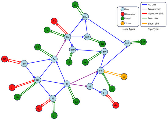
Figure 1. Illustration of the heterogeneous graph representation of the IEEE-14 bus system.

Each node type carries type-specific physical attributes:

• Bus nodes. For each bus $i\in \mathcal{N}$, we store:

  –

  Voltage magnitude limits $(V_i^l,V_i^u)$;

  –

  Base voltage (kV) and bus type (PQ, PV, reference, inactive);

• Generator nodes. Each generator $k\in \mathcal{G}$ is attached to a unique bus $i\left(k\right)\in \mathcal{N}$. For generator node k we store:

  –

  Active/reactive power limits $(P_k^{g,l},P_k^{g,u},Q_k^{g,l},Q_k^{g,u})$;

  –

  Quadratic cost coefficients $(a_k,b_k,c_k)$ defining

  $$C_k\left(P_k^g\right)=a_k{\left(P_k^g\right)}^2+b_k{P}_k^g+c_k;$$

  –

  Initial active/reactive power generation and initial voltage magnitude.

• Load nodes. Each load $k\in \mathcal{L}$ is linked to its bus $i\left(k\right)$ and is characterized by its fixed complex demand

  $$S_k^d=P_k^d+j{Q}_k^d.$$
• Shunt nodes. Each shunt element $k\in \mathcal{S}$ is attached to a bus $i\left(k\right)$ and described by its shunt admittance

  $$Y_k^s=G_k^s+j{B}_k^s.$$
  For a given bus voltage $V_{i\left(k\right)}$, the corresponding shunt injection is $S_k^s={\left(Y_k^s\right)}^{*}{\left|V_{i\left(k\right)}\right|}^2$.

Edge features encode the parameters of physical branches and the auxiliary connector edges:

• AC line edges. For each line $(i,j)\in {\mathcal{E}}^{\mathrm{line}}$ we store:

  –

  Series impedance parameters $(r_{ij},x_{ij})$ with series admittance $Y_{ij}=G_{ij}+j{B}_{ij}={\displaystyle \frac{1}{r_{ij}+j{x}_{ij}}};$

  –

  Shunt (charging) admittances $Y_{ij}^c$ and $Y_{ji}^c$ at the i and j ends of the branch;

  –

  Thermal rating $s_{ij}^u$ (long-term MVA limit), which is used in the branch thermal limit constraint (8);

  –

  Angle-difference limits $(\Delta {\theta }_{ij}^l,\Delta {\theta }_{ij}^u)$ defining the admissible range of $\Delta {\theta }_{ij}$ in (7).

• Transformer edges. For transformer branches $(i,j)\in {\mathcal{E}}^{\mathrm{tr}}$ we store the same electrical parameters as for AC lines, namely $(r_{ij},x_{ij})$, $Y_{ij}$, shunt admittances $(Y_{ij}^c,Y_{ji}^c)$, thermal rating $s_{ij}^u$, and angle-difference limits $(\Delta {\theta }_{ij}^l,\Delta {\theta }_{ij}^u)$. In addition, we store the complex tap ratio $T_{ij}=t_{ij}{e}^{j{\varphi }_{ij}},$ where $t_{ij}$ is the tap magnitude and ${\varphi }_{ij}$ is the phase-shift angle.
• Connector edges. For each generator, load, or shunt node, we create a connector edge to its bus node. These pseudo-edges carry no physical parameters; we only include a small one-hot type indicator that distinguishes generator–bus, load–bus, and shunt–bus connections.

To avoid ambiguity, we use the following conventions throughout the paper: ${\mathcal{G}}^{\mathrm{het}}=(\mathcal{V},{\mathcal{E}}^{\mathrm{het}})$ denotes the heterogeneous graph used by the neural network; $\mathcal{N}$, $\mathcal{G}$, $\mathcal{L}$, and $\mathcal{S}$ denote the sets of buses, generators, loads, and shunts used in the AC-OPF formulation; For each bus i, we denote by ${\mathcal{G}}_i\subset \mathcal{G}$, ${\mathcal{L}}_i\subset \mathcal{L}$, and ${\mathcal{S}}_i\subset \mathcal{S}$ the subsets of generators, loads, and shunts connected to bus i; $S_{ij}$ always denotes the apparent power flow from bus i to bus j, while $s_{ij}^u$ is its thermal rating.

3.3. AC-OPF Mathematical Formulation

We now recall the AC-OPF problem solved by the conventional optimizer and approximated by our neural model. The formulation follows standard practice and is consistent with the OPFData [46] benchmark and related work.

Decision variables: For every generator $k\in \mathcal{G}$ we introduce a complex power

$$S_k^g=P_k^g+j{Q}_k^g,$$

with real-valued decision variables $(P_k^g,Q_k^g)$. For each bus $i\in \mathcal{N}$ we introduce a voltage phasor

$$V_i=\left|V_i\right|e^{j{\theta }_i},$$

parametrized by voltage magnitude $|V_i|$ and phase angle ${\theta }_i$. Branch flows $S_{ij}=P_{ij}+j{Q}_{ij}$ for $(i,j)\in \mathcal{E}$ are deterministically given by the bus voltages and branch parameters through the AC $\pi$-model; they are not independent variables in our formulation.

Objective: The goal of AC-OPF is to find an operating point that minimizes total generation cost:

$$\underset{\{P_k^g,Q_k^g,|V_i|,{\theta }_i\}}{min}\sum _{k\in \mathcal{G}}\left[a_k{\left(P_k^g\right)}^2+b_k{P}_k^g+c_k\right].$$

(1)

Operational constraints: The decision variables are subject to standard engineering limits as follows:

Bus voltage limits:

$$V_i^l\le \left|V_i\right|\le V_i^u,\forall i\in \mathcal{N}.$$

(2)

Generator active and reactive power limits:

$$\begin{array}{cc}\hfill P_k^{g,l}\le P_k^g\le P_k^{g,u},& \forall k\in \mathcal{G},\hfill \end{array}$$

(3)

$$\begin{array}{cc}\hfill Q_k^{g,l}\le Q_k^g\le Q_k^{g,u},& \forall k\in \mathcal{G}.\hfill \end{array}$$

(4)

Reference bus angles: A subset $\mathcal{R}\subseteq \mathcal{N}$ of buses is designated as reference (slack) buses. Their angles are fixed to eliminate the global rotational degree of freedom:

$${\theta }_r=0,\forall r\in \mathcal{R}.$$

(5)

Branch angle difference limits: For each branch $(i,j)\in \mathcal{E}$ we define the effective angle difference

$$\Delta {\theta }_{ij}={\theta }_i-{\theta }_j-{\varphi }_{ij},$$

(6)

where ${\varphi }_{ij}$ is the transformer phase shift (zero for standard AC lines). Operational limits on this angle difference are enforced via

$$\Delta {\theta }_{ij}^l\le \Delta {\theta }_{ij}\le \Delta {\theta }_{ij}^u,\forall (i,j)\in \mathcal{E}.$$

(7)

Branch thermal limits: The apparent power flow on each branch must not exceed its thermal rating:

$$|S_{ij}|\le s_{ij}^u,\forall (i,j)\in \mathcal{E}.$$

(8)

Branch power flow equations: Let $Y_{ij}=1/(r_{ij}+j{x}_{ij})$ denote the series admittance of branch $(i,j)$, and let $Y_{ij}^c$ and $Y_{ji}^c$ denote the shunt (charging) admittances at the i and j ends of the branch, respectively. The complex tap ratio is $T_{ij}=t_{ij}{e}^{j{\varphi }_{ij}}$, with $T_{ij}=1$ for AC lines without transformer taps.

Under the standard AC $\pi$-equivalent model, the complex power flows from bus i to j and from j to i are given by

$$\begin{array}{cc}\hfill S_{ij}& ={(Y_{ij}+Y_{ij}^c)}^{*}{\displaystyle \frac{|V_i{|}^2}{|T_{ij}{|}^2}}-Y_{ij}^{*}{\displaystyle \frac{V_i{V}_j^{*}}{T_{ij}}},\forall (i,j)\in \mathcal{E},\hfill \end{array}$$

(9)

$$\begin{array}{cc}\hfill S_{ji}& ={(Y_{ij}+Y_{ji}^c)}^{*}{\left|V_j\right|}^2-Y_{ij}^{*}{\displaystyle \frac{V_i^{*}{V}_j}{T_{ij}^{*}}},\forall (i,j)\in \mathcal{E}.\hfill \end{array}$$

(10)

Each branch flow can be decomposed into its active and reactive components,

$$S_{ij}=P_{ij}+j{Q}_{ij},S_{ji}=P_{ji}+j{Q}_{ji}.$$

Power balance constraints: Finally, Kirchhoff’s current law is enforced at each bus in complex power form. For each $i\in \mathcal{N}$:

$$\sum _{k\in {\mathcal{G}}_i}{S}_k^g-\sum _{k\in {\mathcal{L}}_i}{S}_k^d-\sum _{k\in {\mathcal{S}}_i}{S}_k^s=\sum _{j:(i,j)\in \mathcal{E}}{S}_{ij},\forall i\in \mathcal{N}.$$

(11)

where the right-hand side collects all branch flows $S_{ij}$ whose sending end is bus i. Equivalently, one may include both outgoing and incoming flows using an incidence-based formulation; in our implementation, the data is oriented so that $\mathcal{E}$ contains a unique directed representation for each physical branch with i as the sending end in (11).

Equations (1)–(11) define the AC-OPF problem that we approximate. Given grid parameters and load profiles, the goal of our neural solver is to predict near-optimal operating points $\left(\right|V|,\theta ,P^g,Q^g)$ that satisfy these constraints up to small residual violations and from which all remaining electrical quantities (branch flows, shunt injections, etc.) can be recovered via the power flow Equations (9) and (10).

4. Methodology

4.1. Model Architecture

The proposed Heterogeneous Graph Neural Network with Local–Global Message Passing (LG-HGNN) learns a supervised approximation of AC-OPF solutions generated by a conventional solver, as defined in Section 3. After given grid parameters and load profiles, LG-HGNN predicts near-optimal values of $\left(\right|V|,\theta ,P^g,Q^g)$. As shown in Figure 2, the architecture follows an encoder–processor–decoder paradigm:

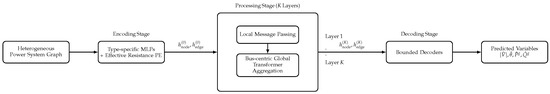
Figure 2. Overall architecture of the proposed LG-HGNN.

• An encoding stage that maps raw heterogeneous node and edge features into a common latent space and augments bus nodes with effective-resistance positional encodings.
• A processing stage comprising K layers that combine local heterogeneous message passing with a bus-centric, effective-resistance-biased global transformer aggregation. This hierarchical design captures short-range electrical interactions while modeling long-range dependencies, such as voltage-angle correlations, in a way that respects the physical role of buses.
• A decoding stage that uses type-specific bounded decoders to produce physically interpretable quantities (generator powers, bus voltages) directly constrained by the operational limits defined in (2)–(4). Remaining variables, such as branch flows $S_{ij}$, are derived deterministically using the power flow Equations (9) and (10).

4.1.1. Encoding Stage

To inject global structural information into node representations, we employ effective resistance as a positional encoding that reflects the electrical distance between buses [55]. Consider the DC power flow linearization

$$P=L\theta ,$$

where $P\in {\mathbb{R}}^N$ collects active power injections at all buses, $\theta \in {\mathbb{R}}^N$ contains voltage angles, and $L\in {\mathbb{R}}^{N\times N}$ is a susceptance-weighted graph Laplacian constructed from nonnegative edge weights $b_{ij}$ (e.g., the magnitudes of line susceptances). Its entries are

$$L_{ij}=\left\{\begin{array}{cc}-b_{ij},\hfill & i\ne j,\hfill \\ {\displaystyle \sum _{k=1}^N}{b}_{ik},\hfill & i=j,\hfill \end{array}\right.$$

(12)

so that each row of L sums to zero and L is positive semidefinite. Let $L^{+}$ denote the Moore–Penrose pseudoinverse of L.

The effective resistance between buses i and j is

$${\Omega }_{ij}={(e_i-e_j)}^{\top }{L}^{+}(e_i-e_j),$$

(13)

with $e_i$ the i-th canonical basis vector. The Laplacian L and effective resistances ${\Omega }_{ij}$ are computed on the bus–bus graph obtained from $\mathcal{E}$.

For each bus i, we summarize its row ${\Omega }_{i,:}$ via simple statistics,

$${\mathrm{PE}}_i=\left[\mathrm{mean}\left({\Omega }_{i,:}\right),\mathrm{std}\left({\Omega }_{i,:}\right),min\left({\Omega }_{i,:}\right),\mathrm{median}\left({\Omega }_{i,:}\right),max\left({\Omega }_{i,:}\right)\right],$$

(14)

yielding a compact, scale-invariant positional encoding that captures the distribution of electrical distances from bus i to the rest of the network.

We then map all heterogeneous node and edge types to a shared latent space using type-specific multilayer perceptrons. Let $a\in \{\mathrm{bus},\mathrm{gen},\mathrm{load},\mathrm{shunt}\}$ index node types, and let $e\in \{\mathrm{line},\mathrm{tr},\mathrm{con}\}$ index edge types. Denote by $x_u^a$ the raw feature vector of node u of type a, and by $x_{(i,j)}^e$ the raw feature vector for an edge $(i,j)$ of type e.

For bus nodes $i\in \mathcal{N}$, we concatenate the effective resistance encoding and apply a type-specific encoder:

$$h_{\mathrm{bus},i}^{\left(0\right)}=\mathrm{LayerNorm}\left({\mathrm{MLP}}_{\mathrm{enc}}^{\mathrm{bus}}\left([x_i^{\mathrm{bus}}\parallel {\mathrm{PE}}_i]\right)\right).$$

(15)

For generator, load, and shunt nodes, we reuse the positional encoding of their host bus $i\left(u\right)$:

$$h_{a,u}^{\left(0\right)}=\mathrm{LayerNorm}\left({\mathrm{MLP}}_{\mathrm{enc}}^a\left([x_u^a\parallel {\mathrm{PE}}_{i\left(u\right)}]\right)\right),a\in \{\mathrm{gen},\mathrm{load},\mathrm{shunt}\}.$$

(16)

For edges, we use edge-type-specific encoders:

$$h_{e,(i,j)}^{\left(0\right)}=\mathrm{LayerNorm}\left({\mathrm{MLP}}_{\mathrm{enc}}^e\left(x_{(i,j)}^e\right)\right).$$

(17)

All encoders are two-layer MLPs with ReLU activations.

4.1.2. Processing Stage: Local and Global Message Passing

The core of LG-HGNN is a stack of K layers that alternates between local heterogeneous message passing and bus-centric global transformer aggregation. The local mechanism captures near-neighbor electrical interactions and respects type-specific relations, while the global transformer operates on bus embeddings to propagate information across the entire grid, reflecting the fact that voltage magnitudes and angles are defined per bus and are globally coupled through the admittance matrix.

At layer k, we denote node and edge embeddings by $h_{\mathrm{node}}^{\left(k\right)}$ and $h_{\mathrm{edge}}^{\left(k\right)}$ for brevity.

Local message passing with edge-aware attention: Each local layer consists of an edge update followed by a node update. A two-stage attention mechanism is employed to handle grid heterogeneity effectively. The edge update stage modulates messages based on joint node–edge–node context, allowing the model to selectively filter interactions according to physical branch attributes such as impedance, tap ratios, and connection type. The node update attention operates during neighborhood aggregation, re-weighting incoming messages to account for competition among multiple neighbors. This separation reflects the heterogeneous electrical roles of branches and nodes: the edge update stage captures relation-specific effects, while the node update stage resolves context-dependent importance among multiple incident components.

Edge update. For an edge $(i,j)$ of type e connecting nodes i and j of types $a\left(i\right)$ and $a\left(j\right)$, we first form an edge message:

$$\begin{array}{cc}\hfill m_{e,(i,j)}^{\left(k\right)}=& {\mathrm{MLP}}_{\mathrm{edge}}^e\left([h_{a\left(i\right),i}^{(k-1)}\parallel h_{e,(i,j)}^{(k-1)}\parallel h_{a\left(j\right),j}^{(k-1)}]\right),\hfill \end{array}$$

(18)

$$\begin{array}{cc}\hfill {\alpha }_{e,(i,j)}^{\left(k\right)}=& \sigma \left({\left(w_e\right)}^{\top }{m}_{e,(i,j)}^{\left(k\right)}\right),\hfill \end{array}$$

(19)

$$\begin{array}{cc}\hfill {\tilde{h}}_{e,(i,j)}^{\left(k\right)}=& {\alpha }_{e,(i,j)}^{\left(k\right)}·m_{e,(i,j)}^{\left(k\right)},\hfill \end{array}$$

(20)

$$\begin{array}{cc}\hfill h_{e,(i,j)}^{\left(k\right)}=& h_{e,(i,j)}^{(k-1)}+\mathrm{Dropout}\left({\tilde{h}}_{e,(i,j)}^{\left(k\right)}\right),\hfill \end{array}$$

(21)

where $\sigma (·)$ is the sigmoid function and $w_e$ is a learnable attention vector specific to edge type e.

Node update. For each node i of type $a\in \{\mathrm{bus},\mathrm{gen},\mathrm{load},\mathrm{shunt}\}$, we aggregate messages over its incident edges $\mathcal{N}\left(i\right)$ (the set of neighbors of node i) using a degree-normalized attention mechanism:

$$\begin{array}{cc}\hfill q_{a,i}^{\left(k\right)}=& W_a^Q{h}_{a,i}^{(k-1)},\hfill \end{array}$$

(22)

$$\begin{array}{cc}\hfill k_{e,(i,j)}^{\left(k\right)}=& W_e^K[h_{a\left(j\right),j}^{(k-1)}\parallel h_{e,(i,j)}^{\left(k\right)}],\hfill \end{array}$$

(23)

$$\begin{array}{cc}\hfill v_{e,(i,j)}^{\left(k\right)}=& W_e^V[h_{a\left(j\right),j}^{(k-1)}\parallel h_{e,(i,j)}^{\left(k\right)}],\hfill \end{array}$$

(24)

$$\begin{array}{cc}\hfill e_{ij}^{\left(k\right)}=& {\displaystyle \frac{{\left(q_{a,i}^{\left(k\right)}\right)}^{\top }{k}_{e,(i,j)}^{\left(k\right)}}{\sqrt{d}}},\hfill \end{array}$$

(25)

$$\begin{array}{cc}\hfill {\alpha }_{ij}^{\left(k\right)}=& {\mathrm{softmax}}_{j\in \mathcal{N}\left(i\right)}\left(e_{ij}^{\left(k\right)}\right),\hfill \end{array}$$

(26)

$$\begin{array}{cc}\hfill m_{a,i}^{\left(k\right)}=& \sum _{j\in \mathcal{N}\left(i\right)}{\displaystyle \frac{{\alpha }_{ij}^{\left(k\right)}}{\sqrt{d_i{d}_j}}}{v}_{e,(i,j)}^{\left(k\right)},\hfill \end{array}$$

(27)

$$\begin{array}{cc}\hfill {\tilde{h}}_{a,i}^{\left(k\right)}=& {\mathrm{MLP}}_{\mathrm{node}}^a\left([h_{a,i}^{(k-1)}\parallel m_{a,i}^{\left(k\right)}]\right),\hfill \end{array}$$

(28)

$$\begin{array}{cc}\hfill h_{a,i}^{\left(k\right)}=& h_{a,i}^{(k-1)}+\mathrm{Dropout}\left({\tilde{h}}_{a,i}^{\left(k\right)}\right),\hfill \end{array}$$

(29)

where $W_a^Q$, $W_e^K$, and $W_e^V$ are learnable projections, d is the latent dimension, and $d_i$ denotes the (possibly normalized) degree of node i. Residual connections and dropout mitigate over-smoothing and stabilize deep message passing.

Bus-centric hierarchical global aggregation: After local updates, we apply a global Transformer only to bus nodes, which serve as the physically meaningful carriers of voltage states. We stack the bus-node embeddings at layer k as

$$H_{\mathrm{bus}}^{\left(k\right)}={\left[h_{\mathrm{bus},i}^{\left(k\right)}\right]}_{i\in \mathcal{N}}.$$

(30)

For each attention head $h=1,\dots ,N_h$, we compute bus-level queries, keys, and values as

$$Q_h=H_{\mathrm{bus}}^{\left(k\right)}{W}_Q^{\left(h\right)},K_h=H_{\mathrm{bus}}^{\left(k\right)}{W}_K^{\left(h\right)},V_h=H_{\mathrm{bus}}^{\left(k\right)}{W}_V^{\left(h\right)}.$$

(31)

To inject electrical-distance priors, we bias the attention logits using the effective resistance ${\Omega }_{ij}$ defined in (13). For buses $i,j\in \mathcal{N}$, the attention score of head h is

$$e_{ij}^{(k,h)}={\displaystyle \frac{Q_{h,i}{K}_{h,j}^{\top }}{\sqrt{d/N_h}}}-\beta {\Omega }_{ij},$$

(32)

where $\beta$ is a learnable or fixed scaling factor controlling the influence of electrical distance. The corresponding attention weights and head outputs are

$${\alpha }_{ij}^{(k,h)}={\mathrm{softmax}}_j\left(e_{ij}^{(k,h)}\right),Z_{h,i}^{\left(k\right)}=\sum _j{\alpha }_{ij}^{(k,h)}{V}_{h,j}.$$

(33)

Outputs from all heads are concatenated and projected:

$$Z_{\mathrm{bus}}^{\left(k\right)}=\mathrm{Concat}\left(Z_1^{\left(k\right)},\dots ,Z_{N_h}^{\left(k\right)}\right)W_O.$$

(34)

A feedforward block with residual connection then yields the global bus update:

$$H_{\mathrm{bus},\mathrm{global}}^{\left(k\right)}=H_{\mathrm{bus}}^{\left(k\right)}+\gamma ·\mathrm{Dropout}\left({\mathrm{MLP}}_{\mathrm{trans}}\left(\mathrm{LayerNorm}\left(Z_{\mathrm{bus}}^{\left(k\right)}\right)\right)\right),$$

(35)

where $\gamma$ is a learnable scaling factor.

The updated bus representations are finally fused back into all node types in a hierarchical fashion. For each bus $i\in \mathcal{N}$,

$$h_{\mathrm{bus},i}^{\left(k\right)}\leftarrow \mathrm{LayerNorm}\left(h_{\mathrm{bus},i}^{\left(k\right)}+W_{\mathrm{bus}}{H}_{\mathrm{bus},\mathrm{global},i}^{\left(k\right)}\right),$$

(36)

and for each generator, load, or shunt node u attached to bus $i\left(u\right)$,

$$h_{a,u}^{\left(k\right)}\leftarrow \mathrm{LayerNorm}\left(h_{a,u}^{\left(k\right)}+W_a{H}_{\mathrm{bus},\mathrm{global},i\left(u\right)}^{\left(k\right)}\right),a\in \{\mathrm{gen},\mathrm{load},\mathrm{shunt}\}.$$

(37)

This bus-centric hierarchical design reduces the quadratic attention complexity to ${\left|\mathcal{N}\right|}^2$ and aligns the modeling of long-range dependencies with the physical role of buses in AC power flow.

4.1.3. Decoding Stage

After K layers of processing, the model produces final node embeddings $h_{a,i}^{\left(K\right)}$ that are decoded into AC-OPF variables. We use type-specific decoders with bounded outputs to enforce box constraints by design.

For each generator node $k\in \mathcal{G}$ we predict active and reactive powers $({\widehat{P}}_k^g,{\widehat{Q}}_k^g)$ as

$${\widehat{y}}_{\mathrm{gen},k}=\mathrm{Scale}\left(\sigma \left({\mathrm{MLP}}_{\mathrm{dec}}^{\mathrm{gen}}\left(h_{\mathrm{gen},k}^{\left(K\right)}\right)\right),y_{\mathrm{gen},k}^l,y_{\mathrm{gen},k}^u\right),$$

(38)

where $\sigma (·)$ is the sigmoid function mapping into $(0,1)$, and $\mathrm{Scale}(x,y^l,y^u)=y^l+x·(y^u-y^l)$ is applied elementwise with $(y_{\mathrm{gen},k}^l,y_{\mathrm{gen},k}^u)$ given by the generator limits $(P_k^{g,l},P_k^{g,u},Q_k^{g,l},Q_k^{g,u})$. This ensures that the box constraints (3) and (4) are satisfied by construction.

For each bus node $i\in \mathcal{N}$ we decode the voltage magnitude $|{\widehat{V}}_i|$ within its bounds:

$$|{\widehat{V}}_i| =\mathrm{Scale}\left(\sigma \left({\mathrm{MLP}}_{\mathrm{dec}}^{\mathrm{bus}}\left(h_{\mathrm{bus},i}^{\left(K\right)}\right)\right),V_i^l,V_i^u\right),$$

(39)

so that (2) holds. Voltage angles ${\widehat{\theta }}_i$ are predicted directly as unconstrained real-valued outputs,

$${\widehat{\theta }}_i={\mathrm{MLP}}_{\mathrm{dec}}^{\theta }\left(h_{\mathrm{bus},i}^{\left(K\right)}\right),$$

(40)

and are subsequently regulated via angle-difference and power-balance penalties in the loss function rather than hard box constraints.

Given $\left(\right|\widehat{V}|,\widehat{\theta })$, we recover complex voltages ${\widehat{V}}_i=\left|{\widehat{V}}_i\right|e^{j{\widehat{\theta }}_i}$ and compute branch flows ${\widehat{S}}_{ij}$ and ${\widehat{S}}_{ji}$ deterministically using the power flow Equations (9) and (10). These derived quantities allow us to evaluate branch thermal limits (8) and power balance (11) without making them additional network outputs.

4.2. Loss Function

We train LG-HGNN to approximate AC-OPF solutions using a composite loss that combines a supervised prediction term with two physics-informed regularizers. The overall training objective is

$$\mathcal{L}={\mathcal{L}}_{\mathrm{pred}}+{\lambda }_1{\mathcal{L}}_{\mathrm{branch}}+{\lambda }_2{\mathcal{L}}_{\mathrm{PF}},$$

(41)

where ${\lambda }_1$ and ${\lambda }_2$ control the trade-off between data fit and physical consistency.

Prediction loss: Given ground-truth AC-OPF solutions $({\theta }_i,|V_i|,P_k^g,Q_k^g,S_{ij},S_{ji})$ from a conventional solver, the prediction loss penalizes mean-squared deviations between the neural outputs and these labels:

$$\begin{array}{cc}\hfill {\mathcal{L}}_{\mathrm{pred}}=& \sum _{i\in \mathcal{N}}\left(\parallel {\widehat{\theta }}_i-{\theta }_i{\parallel }_2^2+\parallel |{\widehat{V}}_i|-|V_i{|\parallel }_2^2\right)+\sum _{k\in \mathcal{G}}\left(\parallel {\widehat{P}}_k^g-P_k^g{\parallel }_2^2+{\parallel {\widehat{Q}}_k^g-Q_k^g\parallel }_2^2\right)\hfill \\ \hfill & +\sum _{(i,j)\in \mathcal{E}}\left(\parallel {\widehat{S}}_{ij}-S_{ij}{\parallel }_2^2+{\parallel {\widehat{S}}_{ji}-S_{ji}\parallel }_2^2\right).\hfill \end{array}$$

(42)

This term directly encourages the network to match the optimizer’s solution across buses, generators, and branches. Although branch power flows $(S_{ij},S_{ji})$ are deterministically derived from predicted bus voltages and angles via the AC power flow Equations (9) and  (10), we intentionally include them in the supervised loss. This redundancy stabilizes the optimization landscape and accelerates convergence, a strategy often employed in physics-informed learning [6,51,52].

Branch constraint violation loss: To promote satisfaction of angle-difference and thermal limits (7)–(8), we penalize violations using a squared hinge function ${\left[x\right]}_{+}=max(x,0)$. For each branch $(i,j)\in \mathcal{E}$ we define the predicted angle difference

$$\Delta {\widehat{\theta }}_{ij}={\widehat{\theta }}_i-{\widehat{\theta }}_j-{\varphi }_{ij},$$

and write

$${\mathcal{L}}_{\mathrm{branch}}=\sum _{(i,j)\in \mathcal{E}}\left({[\Delta {\widehat{\theta }}_{ij}-\Delta {\theta }_{ij}^u]}_{+}^2+{[\Delta {\theta }_{ij}^l-\Delta {\widehat{\theta }}_{ij}]}_{+}^2+\left[\right|{\widehat{S}}_{ij}{|-s_{ij}^u]}_{+}^2\right).$$

(43)

This term encourages the model to remain within operational limits even for samples where such constraints are not explicitly enforced by the supervised labels alone.

Power flow violation loss: Finally, we promote AC feasibility by penalizing violations of the complex power balance (11) at each bus. Using the predicted quantities and the conductance/susceptance entries $G_{ij}^{\mathrm{bus}}$ and $B_{ij}^{\mathrm{bus}}$ of the full bus-admittance matrix $Y^{\mathrm{bus}}$, we first define the active and reactive power mismatches at each bus i as

$$\begin{array}{cc}\hfill P_b^i& =\sum _{k\in {\mathcal{G}}_i}{\widehat{P}}_k^g-\sum _{k\in {\mathcal{L}}_i}{P}_k^d-|{\widehat{V}}_i|\sum _{j\in \mathcal{N}}|{\widehat{V}}_j|\left(G_{ij}^{\mathrm{bus}}cos({\widehat{\theta }}_i-{\widehat{\theta }}_j)+B_{ij}^{\mathrm{bus}}sin({\widehat{\theta }}_i-{\widehat{\theta }}_j)\right),\hfill \end{array}$$

(44)

$$\begin{array}{cc}\hfill Q_b^i& =\sum _{k\in {\mathcal{G}}_i}{\widehat{Q}}_k^g-\sum _{k\in {\mathcal{L}}_i}{Q}_k^d-|{\widehat{V}}_i|\sum _{j\in \mathcal{N}}|{\widehat{V}}_j|\left(G_{ij}^{\mathrm{bus}}sin({\widehat{\theta }}_i-{\widehat{\theta }}_j)-B_{ij}^{\mathrm{bus}}cos({\widehat{\theta }}_i-{\widehat{\theta }}_j)\right),\hfill \end{array}$$

(45)

and then aggregate them into scalar residuals

$$P_b={\displaystyle \frac{1}{\left|\mathcal{N}\right|}}\sum _{i\in \mathcal{N}}|P_b^i|,Q_b={\displaystyle \frac{1}{\left|\mathcal{N}\right|}}\sum _{i\in \mathcal{N}}\left|Q_b^i\right|.$$

(46)

The power flow violation loss is finally defined as

$${\mathcal{L}}_{\mathrm{PF}}=P_b+Q_b.$$

(47)

Minimizing ${\mathcal{L}}_{\mathrm{PF}}$ drives the predicted operating point toward satisfaction of Kirchhoff’s laws and reduces the amount of correction required by a subsequent AC power flow post-processing step. We use an $L_2$ norm for ${\mathcal{L}}_{\mathrm{pred}}$ since it is a supervised regression loss on solver-generated continuous labels, for which squared error is a standard choice. In contrast, ${\mathcal{L}}_{\mathrm{PF}}$ acts as a feasibility regularizer during training, especially in early epochs. The power-flow mismatches can be sparse and heavy-tailed, i.e., a small number of buses may exhibit large residuals. We therefore adopt an $L_1$ aggregation in ${\mathcal{L}}_{\mathrm{PF}}$ to improve robustness to outliers and to prevent a few large mismatches from dominating the gradient signal.

Training Workflow: The overall training workflow of LG-HGNN is summarized in Algorithm 1. Each iteration encodes the heterogeneous graph, performs K layers of local–global message passing with residual updates, decodes the predicted AC-OPF variables, and minimizes the composite loss.

Algorithm 1 Training Procedure of LG-HGNN for AC-OPF Approximation.

Require: Heterogeneous graph ${\mathcal{G}}^{\mathrm{het}}=(\mathcal{V},{\mathcal{E}}^{\mathrm{het}})$; node and edge features $\left\{x_u^a\right\},\left\{x_{(i,j)}^e\right\}$; ground-truth AC-OPF labels $\left(\right|V|,\theta ,P^g,Q^g,S_{ij},S_{ji})$; hyperparameters ${\lambda }_1,{\lambda }_2$.

Ensure: Trained parameters $\Theta$ of LG-HGNN.

1: Initialization: Compute effective-resistance encodings ${\mathrm{PE}}_i$ using Equation (14). Initialize all encoder, processor, and decoder weights $\Theta$.   2: for each training iteration do   3:        (1) Encoding: Obtain initial node and edge embeddings $h_{a,i}^{\left(0\right)},h_{e,(i,j)}^{\left(0\right)}$ via type-specific MLP encoders (Equations (15)–(17)).   4:        (2) Message Passing:   5:        for $k=1,\dots ,K$ do   6:                 (a) Update edges using Equations (18)–(21).   7:                 (b) Update nodes using Equations (22)–(29).   8:                 (c) Compute bus-centric global transformer aggregation using Equations (30)–(35).   9:                 (d) Fuse local and global representations via Equations (36) and (37). 10:        end for 11:        (3) Decoding: Generate predictions $(|\widehat{V}|,\widehat{\theta },{\widehat{P}}^g,{\widehat{Q}}^g)$ using bounded decoders (Equations (38)–(40)); compute derived branch flows ${\widehat{S}}_{ij}$ and ${\widehat{S}}_{ji}$ via the power flow Equations (9) and (10). 12:        (4) Compute Loss: Evaluate prediction loss ${\mathcal{L}}_{\mathrm{pred}}$ (Equation (42)), branch constraint loss ${\mathcal{L}}_{\mathrm{branch}}$ (Equation (43)), and power-flow violation loss ${\mathcal{L}}_{\mathrm{PF}}$ (Equations (44)–(47)); form the total loss $\mathcal{L}$ as in Equation (41). 13:        (5) Parameter Update: Backpropagate through all modules and update $\Theta$ using the Adam optimizer. 14:  end for

In summary, LG-HGNN combines heterogeneous graph modeling, bus-centric local–global message passing with effective-resistance-biased attention, bounded decoding, and physics-informed regularization to learn a fast and topology-robust surrogate of the AC-OPF optimizer that produces near-feasible and near-optimal dispatches directly from the underlying network data.

5. Experimental Evaluation

5.1. Datasets

We evaluate the proposed LG-HGNN framework on the OPFData dataset [46], which is currently the largest publicly available open-source AC-OPF dataset and contains 300,000 solved instances per grid configuration obtained with AC-IPOPT. The dataset encompasses 10 distinct grid topologies from the Power Grid Library [45]. Each grid topology includes two dataset variants: (1) ‘Full topology’ featuring the default grid configuration with active and reactive loads varying independently by $\pm 20\%$ of nominal values, and (2) ‘N-1 topology’ where each instance has a randomly disconnected component (either branch or generator). For our experimental analysis, we utilize representative grids: IEEE-14, IEEE-30, IEEE-118. We further include the medium-scale GOC-2000 system from OPFData to assess the scalability of LG-HGNN to grids with 2000 buses and highly heterogeneous topology.

5.2. Baseline Models

To evaluate the effectiveness of the proposed LG-HGNN, we compare it with one classical optimization solver and two representative graph neural networks:

• DC-IPOPT: An efficient framework for large-scale nonconvex optimization. It combines a sequential convex approximation outer loop with an interior-point solver (IPOPT) inner loop to iteratively handle nonlinear constraints. This decomposition enhances robustness and convergence stability, enabling DC-IPOPT to serve as a strong baseline for AC-OPF approximation.
• Graph Attention Network (GAT): A neural model that integrates the attention mechanism into neighborhood aggregation. By assigning learnable importance weights to neighboring nodes, GAT adaptively captures salient local structures while maintaining inductive learning capability and strong generalization across varying graph topologies.
• Graph Isomorphism Network (GIN): A theoretically grounded GNN proven to match the expressive power of the Weisfeiler–Lehman graph isomorphism test. Using a sum-based injective aggregation and an MLP update, GIN distinguishes fine structural variations in graphs and serves as a powerful baseline for graph representation learning.

All neural baselines (GAT, GIN) are trained under the same physics-aware loss function and constraint regularization. Their predictions thus constitute OPF-feasible warm-start candidates for classical solvers. The PF-corrected results effectively represent the hybrid GNN + OPF refinement stage, enabling a fair comparison of the physical consistency across models.

5.3. Experimental Configuration

Dataset partitioning allocates 270,000 samples for training ($90\%$), 15,000 for validation ($5\%$), and 15,000 for testing ($5\%$). Batch sizes are set to 256. For DC-IPOPT, the approximate solution is generated using the open-source Julia package PowerModels.jl [45] with the Ipopt optimizer. For the GAT and GIN baselines, we use the same composite loss function as LG-HGNN and set both models to have 3 layers with a hidden dimension of 256. Both models are trained using the Adam optimizer with a learning rate of $1\times {10}^{-5}$ and weight decay of $1\times {10}^{-5}$ for 200 epochs. For the proposed LG-HGNN, we also use the Adam optimizer with early stopping and gradient clipping for stability, a learning rate of $5\times {10}^{-5}$, and weight decay of $5\times {10}^{-5}$ for 200 epochs. We set ${\lambda }_1=0.7$ and ${\lambda }_2=0.3$ in the composite loss. We also set $K=3$ with a consistent hidden dimension of 256 for all datasets.

5.4. Evaluation Metrics

We assess model performance using three complementary metrics: (1) Mean Squared Error (MSE), which computes the mean of squared differences between predictions and ground-truth values for each AC-OPF variable. (2) Feasibility, quantified by the average degree of constraint violations for Equations (7), (8) and (11), which are not strictly enforced during training. Generator power and voltage magnitude constraints (Equations (2)–(4)) are satisfied by design through our constrained decoding approach. All violation magnitudes are averaged over the test set. (3) Optimality ratio, defined as the ratio (in percent) between the objective cost computed from model predictions and the ground-truth AC-OPF cost.

5.5. Post-Processing Predictions with Power Flow

Power flow analysis can be applied to post-process the raw predictions from machine-learning solvers, ensuring that the resulting solutions satisfy Kirchhoff’s power balance constraints (see Equation (11)) and are AC-feasible. In this step, the predicted bus voltages and generator setpoints are used as initialization for an AC power flow solver (e.g., pandapower with numba acceleration), which computes consistent active and reactive flows across all branches. As detailed in [22], this post-processing guarantees satisfaction of the bus complex power balance equation, but other inequality constraints may still be violated. Specifically, only the slack bus adjusts its active power output to restore system-wide balance, which may lead to violations of its generation bounds. The active and reactive generations at other PV buses remain fixed as predicted by the ML model, while the reactive power at PQ buses may change to satisfy voltage and network constraints. Reactive power limits are not enforced by default; however, these can be incorporated by dynamically converting PV buses that reach their reactive power limits into PQ buses. Overall, the power flow post-processing step serves as a lightweight feasibility restoration procedure that significantly improves the physical consistency of ML-based OPF predictions.

5.6. Performance Comparison on Full Topology

Table 2, Table 3 and Table 4 comprehensively summarize model performance on the full-topology datasets (14-, 30-, and 118-bus systems) before and after AC power flow post-processing. Overall, LG-HGNN (Our_F) consistently matches or outperforms all baselines across almost all variables and grid sizes, while DC-IPOPT frequently exhibits poor AC feasibility once its DC solution is embedded into the full AC network.

Table 2. MSE of baselinesand LG-HGNN across different grid sizes on ’Full topology’. The non-shaded rows are pre-power flow results, while the shaded rows are post-power flow results.

		IEEE-14				IEEE-30				IEEE-118
		DC-IPOPT	GAT	GIN	OurF	DC-IPOPT	GAT	GIN	OurF	DC-IPOPT	GAT	GIN	OurF
Bus	$\theta$	$4.38\times {10}^{-3}$	$1.50\times {10}^{-5}$	$2.00\times {10}^{-5}$	$1.50\times {10}^{-6}$	$2.13\times {10}^{-2}$	$3.65\times {10}^{-5}$	$4.00\times {10}^{-5}$	$3.22\times {10}^{-5}$	$1.29\times {10}^{-2}$	$1.49\times {10}^{-4}$	$1.60\times {10}^{-4}$	$1.48\times {10}^{-4}$
		$4.35\times {10}^{-3}$	$1.55\times {10}^{-5}$	$2.10\times {10}^{-5}$	$1.48\times {10}^{-6}$	$2.14\times {10}^{-2}$	$3.70\times {10}^{-5}$	$4.10\times {10}^{-5}$	$3.20\times {10}^{-5}$	$1.29\times {10}^{-2}$	$1.50\times {10}^{-4}$	$1.62\times {10}^{-4}$	$1.47\times {10}^{-4}$
	$\left|V\right|$	$5.13\times {10}^{-3}$	$3.12\times {10}^{-6}$	$4.00\times {10}^{-6}$	$3.12\times {10}^{-6}$	$4.57\times {10}^{-3}$	$3.73\times {10}^{-6}$	$4.00\times {10}^{-6}$	$1.90\times {10}^{-6}$	$5.03\times {10}^{-3}$	$1.65\times {10}^{-5}$	$1.70\times {10}^{-5}$	$1.50\times {10}^{-5}$
		$5.12\times {10}^{-3}$	$3.15\times {10}^{-6}$	$4.10\times {10}^{-6}$	$3.10\times {10}^{-6}$	$4.57\times {10}^{-3}$	$3.75\times {10}^{-6}$	$4.05\times {10}^{-6}$	$1.88\times {10}^{-6}$	$5.03\times {10}^{-3}$	$1.66\times {10}^{-5}$	$1.72\times {10}^{-5}$	$1.48\times {10}^{-5}$
Gen	$P^g$	$6.80\times {10}^{-3}$	$5.79\times {10}^{-5}$	$6.00\times {10}^{-5}$	$5.79\times {10}^{-5}$	$1.41\times {10}^{-2}$	$3.64\times {10}^{-4}$	$3.80\times {10}^{-4}$	$3.17\times {10}^{-4}$	$1.99\times {10}^{-2}$	$4.88\times {10}^{-4}$	$5.00\times {10}^{-4}$	$4.77\times {10}^{-4}$
		$6.74\times {10}^{-3}$	$5.80\times {10}^{-5}$	$6.10\times {10}^{-5}$	$5.78\times {10}^{-5}$	$1.41\times {10}^{-2}$	$3.66\times {10}^{-4}$	$3.82\times {10}^{-4}$	$3.16\times {10}^{-4}$	$1.99\times {10}^{-2}$	$4.90\times {10}^{-4}$	$5.05\times {10}^{-4}$	$4.76\times {10}^{-4}$
	$Q^g$	-	$1.01\times {10}^{-5}$	$1.20\times {10}^{-5}$	$1.01\times {10}^{-5}$	-	$9.67\times {10}^{-4}$	$1.00\times {10}^{-3}$	$7.88\times {10}^{-4}$	-	$1.29\times {10}^{-3}$	$1.35\times {10}^{-3}$	$1.23\times {10}^{-3}$
		$1.82\times {10}^{-1}$	$1.02\times {10}^{-5}$	$1.22\times {10}^{-5}$	$1.00\times {10}^{-5}$	$1.91\times {10}^{-1}$	$9.70\times {10}^{-4}$	$1.02\times {10}^{-3}$	$7.85\times {10}^{-4}$	$1.11\times {10}^{-1}$	$1.30\times {10}^{-3}$	$1.36\times {10}^{-3}$	$1.22\times {10}^{-3}$
Line	$P_{ij}$	$6.28\times {10}^{-3}$	$5.02\times {10}^{-4}$	$6.00\times {10}^{-4}$	$1.10\times {10}^{-4}$	$1.70\times {10}^{-2}$	$5.46\times {10}^{-4}$	$6.00\times {10}^{-4}$	$3.67\times {10}^{-4}$	$1.40\times {10}^{-2}$	$1.25\times {10}^{-3}$	$1.30\times {10}^{-3}$	$1.28\times {10}^{-3}$
		$4.27\times {10}^{-2}$	$5.05\times {10}^{-4}$	$6.10\times {10}^{-4}$	$1.09\times {10}^{-4}$	$7.68\times {10}^{-2}$	$5.48\times {10}^{-4}$	$6.05\times {10}^{-4}$	$3.65\times {10}^{-4}$	$6.86\times {10}^{-2}$	$1.26\times {10}^{-3}$	$1.32\times {10}^{-3}$	$1.27\times {10}^{-3}$
	$P_{ji}$	$6.38\times {10}^{-3}$	$5.03\times {10}^{-4}$	$6.10\times {10}^{-4}$	$1.10\times {10}^{-4}$	$1.71\times {10}^{-2}$	$5.45\times {10}^{-4}$	$6.10\times {10}^{-4}$	$3.66\times {10}^{-4}$	$1.43\times {10}^{-2}$	$1.25\times {10}^{-3}$	$1.31\times {10}^{-3}$	$1.28\times {10}^{-3}$
		$3.17\times {10}^{-2}$	$5.06\times {10}^{-4}$	$6.12\times {10}^{-4}$	$1.08\times {10}^{-4}$	$1.12\times {10}^{-1}$	$5.47\times {10}^{-4}$	$6.08\times {10}^{-4}$	$3.64\times {10}^{-4}$	$5.51\times {10}^{-2}$	$1.26\times {10}^{-3}$	$1.33\times {10}^{-3}$	$1.27\times {10}^{-3}$
	$Q_{ij}$	-	$2.58\times {10}^{-5}$	$3.00\times {10}^{-5}$	$1.21\times {10}^{-5}$	-	$4.00\times {10}^{-4}$	$4.50\times {10}^{-4}$	$3.04\times {10}^{-4}$	-	$1.28\times {10}^{-3}$	$1.35\times {10}^{-3}$	$1.17\times {10}^{-3}$
		$3.20\times {10}^{-2}$	$2.60\times {10}^{-5}$	$3.10\times {10}^{-5}$	$1.20\times {10}^{-5}$	$1.14\times {10}^{-1}$	$4.02\times {10}^{-4}$	$4.55\times {10}^{-4}$	$3.02\times {10}^{-4}$	$5.52\times {10}^{-2}$	$1.29\times {10}^{-3}$	$1.36\times {10}^{-3}$	$1.16\times {10}^{-3}$
	$Q_{ji}$	-	$2.56\times {10}^{-5}$	$3.10\times {10}^{-5}$	$1.21\times {10}^{-5}$	-	$4.01\times {10}^{-4}$	$4.60\times {10}^{-4}$	$3.05\times {10}^{-4}$	-	$1.28\times {10}^{-3}$	$1.36\times {10}^{-3}$	$1.17\times {10}^{-3}$
		$3.82\times {10}^{-2}$	$2.58\times {10}^{-5}$	$3.12\times {10}^{-5}$	$1.19\times {10}^{-5}$	$7.52\times {10}^{-2}$	$4.03\times {10}^{-4}$	$4.58\times {10}^{-4}$	$3.03\times {10}^{-4}$	$6.84\times {10}^{-2}$	$1.29\times {10}^{-3}$	$1.37\times {10}^{-3}$	$1.16\times {10}^{-3}$
Trans.	$P_{ij}$	$7.22\times {10}^{-3}$	$2.30\times {10}^{-4}$	$2.50\times {10}^{-4}$	$6.47\times {10}^{-5}$	$4.28\times {10}^{-3}$	$1.81\times {10}^{-4}$	$2.00\times {10}^{-4}$	$1.44\times {10}^{-4}$	$2.25\times {10}^{-2}$	$7.79\times {10}^{-4}$	$8.00\times {10}^{-4}$	$7.53\times {10}^{-4}$
		$1.72\times {10}^{-1}$	$2.32\times {10}^{-4}$	$2.52\times {10}^{-4}$	$6.45\times {10}^{-5}$	$8.29\times {10}^{-2}$	$1.82\times {10}^{-4}$	$2.02\times {10}^{-4}$	$1.43\times {10}^{-4}$	$1.05\times {10}^{-1}$	$7.81\times {10}^{-4}$	$8.05\times {10}^{-4}$	$7.51\times {10}^{-4}$
	$P_{ji}$	$7.30\times {10}^{-3}$	$2.31\times {10}^{-4}$	$2.60\times {10}^{-4}$	$6.49\times {10}^{-5}$	$4.32\times {10}^{-3}$	$1.81\times {10}^{-4}$	$2.10\times {10}^{-4}$	$1.44\times {10}^{-4}$	$2.26\times {10}^{-2}$	$7.82\times {10}^{-4}$	$8.10\times {10}^{-4}$	$7.56\times {10}^{-4}$
		$9.36\times {10}^{-2}$	$2.33\times {10}^{-4}$	$2.62\times {10}^{-4}$	$6.48\times {10}^{-5}$	$1.38\times {10}^{-1}$	$1.83\times {10}^{-4}$	$2.12\times {10}^{-4}$	$1.42\times {10}^{-4}$	$2.14\times {10}^{-1}$	$7.83\times {10}^{-4}$	$8.12\times {10}^{-4}$	$7.54\times {10}^{-4}$
	$Q_{ij}$	-	$1.98\times {10}^{-5}$	$2.20\times {10}^{-5}$	$9.61\times {10}^{-6}$	-	$2.76\times {10}^{-4}$	$3.00\times {10}^{-4}$	$2.40\times {10}^{-4}$	-	$1.38\times {10}^{-3}$	$1.45\times {10}^{-3}$	$1.30\times {10}^{-3}$
		$9.29\times {10}^{-2}$	$2.00\times {10}^{-5}$	$2.22\times {10}^{-5}$	$9.60\times {10}^{-6}$	$1.37\times {10}^{-1}$	$2.78\times {10}^{-4}$	$3.02\times {10}^{-4}$	$2.38\times {10}^{-4}$	$2.12\times {10}^{-1}$	$1.39\times {10}^{-3}$	$1.46\times {10}^{-3}$	$1.29\times {10}^{-3}$
	$Q_{ji}$	-	$1.94\times {10}^{-5}$	$2.10\times {10}^{-5}$	$9.44\times {10}^{-6}$	-	$2.78\times {10}^{-4}$	$3.10\times {10}^{-4}$	$2.42\times {10}^{-4}$	-	$1.40\times {10}^{-3}$	$1.48\times {10}^{-3}$	$1.32\times {10}^{-3}$
		$1.52\times {10}^{-1}$	$1.96\times {10}^{-5}$	$2.12\times {10}^{-5}$	$9.42\times {10}^{-6}$	$7.90\times {10}^{-2}$	$2.80\times {10}^{-4}$	$3.05\times {10}^{-4}$	$2.40\times {10}^{-4}$	$9.31\times {10}^{-2}$	$1.41\times {10}^{-3}$	$1.49\times {10}^{-3}$	$1.31\times {10}^{-3}$

Table 3. Feasibility of baselinesand LG-HGNN across different grid sizes on ’Full topology’. The non-shaded rows are pre-power flow results, while the shaded rows are post-power flow results.

	IEEE-14				IEEE-30				IEEE-118
	DC-IPOPT	GAT	GIN	OurF	DC-IPOPT	GAT	GIN	OurF	DC-IPOPT	GAT	GIN	OurF
$S_{ij}$	-	$4.39\times {10}^{-7}$	$6.00\times {10}^{-7}$	$4.39\times {10}^{-7}$	-	$2.60\times {10}^{-6}$	$4.00\times {10}^{-6}$	$2.60\times {10}^{-6}$	-	$5.09\times {10}^{-7}$	$7.00\times {10}^{-7}$	$5.09\times {10}^{-7}$
	$2.26\times {10}^{-2}$	$5.24\times {10}^{-6}$	$7.00\times {10}^{-6}$	$5.24\times {10}^{-6}$	$1.10\times {10}^{-1}$	$3.11\times {10}^{-5}$	$4.00\times {10}^{-5}$	$3.11\times {10}^{-5}$	$6.55\times {10}^{-2}$	$1.36\times {10}^{-5}$	$1.80\times {10}^{-5}$	$1.36\times {10}^{-5}$
$S_{ji}$	-	$4.83\times {10}^{-6}$	$6.00\times {10}^{-6}$	$4.83\times {10}^{-6}$	-	$2.14\times {10}^{-7}$	$3.00\times {10}^{-7}$	$2.14\times {10}^{-7}$	-	$2.24\times {10}^{-7}$	$3.50\times {10}^{-7}$	$2.24\times {10}^{-7}$
	$3.60\times {10}^{-2}$	$3.17\times {10}^{-7}$	$4.00\times {10}^{-7}$	$3.17\times {10}^{-7}$	$1.17\times {10}^{-1}$	$4.59\times {10}^{-5}$	$6.00\times {10}^{-5}$	$4.59\times {10}^{-5}$	$6.65\times {10}^{-2}$	$8.42\times {10}^{-6}$	$1.10\times {10}^{-5}$	$8.42\times {10}^{-6}$
$\Delta {\theta }_{ij}$	-	$0.00\times {10}^{+0}$	$0.00\times {10}^{+0}$	$0.00\times {10}^{+0}$	-	$0.00\times {10}^{+0}$	$0.00\times {10}^{+0}$	$0.00\times {10}^{+0}$	-	$3.05\times {10}^{-10}$	$5.00\times {10}^{-10}$	$0.00\times {10}^{+0}$
	$0.00\times {10}^{+0}$	$0.00\times {10}^{+0}$	$0.00\times {10}^{+0}$	$0.00\times {10}^{+0}$	$0.00\times {10}^{+0}$	$0.00\times {10}^{+0}$	$0.00\times {10}^{+0}$	$0.00\times {10}^{+0}$	$0.00\times {10}^{+0}$	$0.00\times {10}^{+0}$	$0.00\times {10}^{+0}$	$0.00\times {10}^{+0}$
$P_b$	-	$5.30\times {10}^{-3}$	$6.00\times {10}^{-3}$	$5.30\times {10}^{-3}$	-	$1.08\times {10}^{-2}$	$1.20\times {10}^{-2}$	$9.11\times {10}^{-3}$	-	$2.40\times {10}^{-2}$	$2.70\times {10}^{-2}$	$2.40\times {10}^{-2}$
	$0.00\times {10}^{+0}$	$0.00\times {10}^{+0}$	$0.00\times {10}^{+0}$	$0.00\times {10}^{+0}$	$0.00\times {10}^{+0}$	$0.00\times {10}^{+0}$	$0.00\times {10}^{+0}$	$0.00\times {10}^{+0}$	$0.00\times {10}^{+0}$	$0.00\times {10}^{+0}$	$0.00\times {10}^{+0}$	$0.00\times {10}^{+0}$
$Q_b$	-	$1.82\times {10}^{-3}$	$2.50\times {10}^{-3}$	$1.82\times {10}^{-3}$	-	$5.35\times {10}^{-3}$	$6.00\times {10}^{-3}$	$4.20\times {10}^{-3}$	-	$7.98\times {10}^{-3}$	$9.00\times {10}^{-3}$	$7.98\times {10}^{-3}$
	$0.00\times {10}^{+0}$	$0.00\times {10}^{+0}$	$0.00\times {10}^{+0}$	$0.00\times {10}^{+0}$	$0.00\times {10}^{+0}$	$0.00\times {10}^{+0}$	$0.00\times {10}^{+0}$	$0.00\times {10}^{+0}$	$0.00\times {10}^{+0}$	$0.00\times {10}^{+0}$	$0.00\times {10}^{+0}$	$0.00\times {10}^{+0}$

Table 4. Optimality ratio (%) of baselines and LG-HGNN across different grid sizes on ’Full topology’. The non-shaded rows are pre-power flow results, while the shaded rows are post-power flow results.

	DC-IPOPT	GAT	GIN	OurF
IEEE-14	96.75	101.15	100.95	100.35
	97.90	100.85	100.68	100.25
IEEE-30	95.15	101.85	101.45	100.75
	96.55	101.35	101.15	100.55
IEEE-118	93.80	102.45	102.05	101.15
	95.20	101.95	101.65	100.95

Prediction Accuracy Analysis (Table 2). For bus-level variables, LG-HGNN achieves the lowest or near-lowest MSE for both voltage angles $\theta$ and magnitudes $\left|V\right|$ across all IEEE systems. On the 14-bus grid, the pre-PF MSE for $\theta$ decreases from $4.38\times {10}^{-3}$ (DC-IPOPT) to ${10}^{-5}$ with GAT/GIN and further to $1.5\times {10}^{-6}$ with LG-HGNN, a pattern consistent for 30- and 118-bus systems. For $\left|V\right|$, all neural models significantly outperform DC-IPOPT, with LG-HGNN and GAT typically yielding the smallest errors, demonstrating the stabilizing effect of physics-informed regularization.

For generator variables, LG-HGNN consistently attains the best or tied-best MSE for both $P^g$ and $Q^g$. While GAT and GIN already reduce $P_G$ errors by two orders of magnitude over DC-IPOPT, LG-HGNN further improves them, and its explicit modeling of generator nodes enhances the coupling between reactive power and voltage regulation.

For line and transformer flows ($P_{ij},P_{ji},Q_{ij},Q_{ji}$), DC-IPOPT exhibits large post-PF errors (up to $\mathcal{O}\left({10}^{-1}\right)$), reflecting the DC–AC mismatch. GAT and GIN reduce these errors to ${10}^{-4}$–${10}^{-3}$, while LG-HGNN reaches the ${10}^{-5}$ range, particularly excelling on transformer flows. This demonstrates that heterogeneous representations with global attention enable LG-HGNN to capture long-range power-flow dependencies beyond the capacity of DC-IPOPT or conventional GNNs.

Power-flow post-processing (shaded rows) affects each method differently: LG-HGNN’s MSE changes only slightly, showing its predictions are already close to AC-feasible solutions, whereas DC-IPOPT exhibits large deviations in flow-related variables, confirming that its computational simplicity comes at the cost of AC accuracy.

Constraint Violation Degree Analysis (Table 3). The table reports average violations for key constraints, including branch thermal limits ($S_{ij}$, $S_{ji}$), angle-difference limits $\Delta {\theta }_{ij}$, and active/reactive power balance ($P_b$, $Q_b$). Voltage and generator bounds are excluded since they are directly enforced by constrained decoding.

Before power-flow post-processing (non-shaded rows), all neural models show minimal violations (${10}^{-7}$–${10}^{-2}$), with LG-HGNN matching or surpassing the best baseline. For example, on the 118-bus system, the pre-PF thermal-limit violation $S_{ij}$ is about ${10}^{-7}$ for LG-HGNN, while $P_b$ and $Q_b$ remain within ${10}^{-2}$–${10}^{-3}$ pu, indicating that physics-informed loss promotes Kirchhoff-consistent solutions even without PF correction.

After power flow (shaded rows), differences with DC-IPOPT become pronounced. Because DC-IPOPT ignores reactive power and voltage constraints, its post-PF thermal violations reach $\mathcal{O}\left({10}^{-1}\right)$, whereas LG-HGNN and other GNNs remain in the ${10}^{-5}$–${10}^{-4}$ range. Power-balance errors are reduced to numerical zero for all methods after PF. Overall, LG-HGNN produces solutions inherently closer to AC-feasible operating points than DC-IPOPT, demonstrating superior physical consistency.

Optimality Ratio Analysis (Table 4). The updated results reveal that the proposed LG-HGNN achieves the most economically consistent performance among all solvers. Before power-flow correction, DC-IPOPT yields markedly lower optimality ratios—approximately 96–$97\%$ on the 14- and 30-bus systems and $93.8\%$ on the 118-bus grid—indicating that the DC approximation systematically underestimates the true AC generation cost. After AC power-flow recalculation, its ratios improve slightly but remain well below $100\%$, confirming that DC-based dispatches are economically sub-optimal when evaluated in the nonlinear AC domain.

In contrast, all neural solvers achieve ratios very close to the AC-OPF optimum. GAT and GIN exhibit slightly super-unit ratios (101–$102\%$) across all networks, while LG-HGNN consistently produces the lowest deviation from $100\%$. Specifically, Our_F attains $100.35\%$, $100.75\%$, and $101.15\%$ on the IEEE-14, 30-, and 118-bus cases, respectively, and further stabilizes near $100.25$–$100.95\%$ after PF. These near-unity ratios indicate that LG-HGNN accurately reconstructs generation dispatches that are economically very close to the ground-truth AC-OPF solutions, with minimal numerical bias.

As network size increases, the gap between DC-IPOPT and the neural methods widens, highlighting the scalability and robustness of the proposed architecture. Overall, the full-topology experiments confirm that LG-HGNN effectively balances physical feasibility and economic optimality, correcting the systematic cost bias of DC approximations and surpassing GAT and GIN in both accuracy and consistency across all grid scales.

Scalability to Large-Scale Grids

To evaluate the scalability of the proposed LG-HGNN architecture on realistic large-scale power systems, we further conduct experiments on the GOC-2000 dataset, which contains 2000 buses and exhibits significantly higher topological heterogeneity than the IEEE benchmarks. Table 5 reports the MSE values before and after PF correction for bus voltages, generator outputs, and line flows.

Table 5. MSE of baselines and LG-HGNN on GOC-2000 (Full topology). Non-shaded rows are before PF; shaded rows are after PF.

		DC-IPOPT	GAT	GIN	OurF
Bus	$\theta$	$5.20\times {10}^{-4}$	$3.15\times {10}^{-4}$	$3.40\times {10}^{-4}$	$2.25\times {10}^{-4}$
	$\theta$ (PF)	$3.80\times {10}^{-4}$	$2.10\times {10}^{-4}$	$2.35\times {10}^{-4}$	$1.45\times {10}^{-4}$
	$\left|V\right|$	$5.40\times {10}^{-5}$	$3.90\times {10}^{-5}$	$4.10\times {10}^{-5}$	$2.95\times {10}^{-5}$
	$\left|V\right|$ (PF)	$3.60\times {10}^{-5}$	$2.60\times {10}^{-5}$	$2.80\times {10}^{-5}$	$1.85\times {10}^{-5}$
Gen	$P^g$	$7.80\times {10}^{-4}$	$5.85\times {10}^{-4}$	$6.10\times {10}^{-4}$	$4.95\times {10}^{-4}$
	$P^g$ (PF)	$5.10\times {10}^{-4}$	$3.90\times {10}^{-4}$	$4.10\times {10}^{-4}$	$3.20\times {10}^{-4}$
	$Q^g$	$1.10\times {10}^{-3}$	$8.50\times {10}^{-4}$	$9.20\times {10}^{-4}$	$7.40\times {10}^{-4}$
	$Q^g$ (PF)	$7.40\times {10}^{-4}$	$5.80\times {10}^{-4}$	$6.10\times {10}^{-4}$	$4.80\times {10}^{-4}$
Line	$P_{ij}$	$2.95\times {10}^{-3}$	$1.92\times {10}^{-3}$	$2.05\times {10}^{-3}$	$1.58\times {10}^{-3}$
	$P_{ij}$ (PF)	$1.95\times {10}^{-3}$	$1.25\times {10}^{-3}$	$1.35\times {10}^{-3}$	$1.02\times {10}^{-3}$
	$Q_{ij}$	$3.10\times {10}^{-3}$	$2.05\times {10}^{-3}$	$2.20\times {10}^{-3}$	$1.70\times {10}^{-3}$
	$Q_{ij}$ (PF)	$2.05\times {10}^{-3}$	$1.35\times {10}^{-3}$	$1.45\times {10}^{-3}$	$1.10\times {10}^{-3}$

Across all state variables, LG-HGNN (Our_F) consistently achieves the lowest MSE among the learning-based baselines. On this 2000-bus system, the model maintains high accuracy with only moderate error growth relative to the 118-bus case (e.g., bus-angle MSE before PF increases from $1.48\times {10}^{-4}$ to $2.25\times {10}^{-4}$). After PF correction, all models benefit from enforcing the nonlinear AC power flow equations, and the errors of LG-HGNN are further reduced by approximately 35–40% across most variables (e.g., bus-angle MSE decreases from $2.25\times {10}^{-4}$ to $1.45\times {10}^{-4}$). This indicates that the predictions produced by LG-HGNN are already close to the AC-feasible manifold and require only small corrective adjustments.

Overall, these results demonstrate that LG-HGNN generalizes effectively to large-scale transmission networks with thousands of buses: it preserves its accuracy advantage over GAT and GIN on GOC-2000, while remaining fully compatible with standard PF-based post-processing. This validates the proposed model as a scalable and physically consistent surrogate for real-time AC-OPF applications on realistic, highly heterogeneous grids.

5.7. Performance Comparison on N-1 Topology

The N-1 contingency experiments evaluate the ability of different methods to generalize across large families of perturbed topologies where either a branch or a generator is randomly removed from service. In this setting, we distinguish between two configurations of our model: (1) Our_F, trained only on full-topology data and evaluated zero-shot on N-1 contingencies; and (2) Our_N, fine-tuned directly on the N-1 training subset. Table 6, Table 7 and Table 8 report prediction accuracy, feasibility, and economic optimality across IEEE-14, -30, and -118 systems.

Table 6. MSE of baselines, Our_F and Our_N across different grid sizes on ‘N-1 topology’. The non-shaded rows are pre-power flow results, while the shaded rows are post-power flow results.

		IEEE-14					IEEE-30					IEEE-118
		DC-IPOPT	GAT	GIN	OurF	OurN	DC-IPOPT	GAT	GIN	OurF	OurN	DC-IPOPT	GAT	GIN	OurF	OurN
Bus	$\theta$	$4.35\times {10}^{-3}$	$1.59\times {10}^{-4}$	$2.00\times {10}^{-4}$	$4.70\times {10}^{-5}$	$4.50\times {10}^{-5}$	$2.14\times {10}^{-2}$	$1.16\times {10}^{-4}$	$1.30\times {10}^{-4}$	$1.06\times {10}^{-4}$	$1.04\times {10}^{-4}$	$1.29\times {10}^{-2}$	$1.61\times {10}^{-4}$	$1.80\times {10}^{-4}$	$1.60\times {10}^{-4}$	$1.58\times {10}^{-4}$
		$4.35\times {10}^{-3}$	$4.02\times {10}^{-4}$	$4.50\times {10}^{-4}$	$1.74\times {10}^{-4}$	$1.70\times {10}^{-4}$	$2.14\times {10}^{-2}$	$1.59\times {10}^{-3}$	$1.80\times {10}^{-3}$	$1.39\times {10}^{-3}$	$1.36\times {10}^{-3}$	$1.29\times {10}^{-2}$	$6.00\times {10}^{-4}$	$6.50\times {10}^{-4}$	$6.09\times {10}^{-4}$	$6.00\times {10}^{-4}$
	$\left|V\right|$	$5.12\times {10}^{-3}$	$1.45\times {10}^{-6}$	$1.80\times {10}^{-6}$	$7.10\times {10}^{-6}$	$1.05\times {10}^{-6}$	$4.57\times {10}^{-3}$	$6.07\times {10}^{-6}$	$7.00\times {10}^{-6}$	$2.90\times {10}^{-6}$	$2.85\times {10}^{-6}$	$5.03\times {10}^{-3}$	$1.84\times {10}^{-5}$	$2.00\times {10}^{-5}$	$2.60\times {10}^{-5}$	$1.58\times {10}^{-5}$
		$5.12\times {10}^{-3}$	$1.30\times {10}^{-6}$	$1.60\times {10}^{-6}$	$1.10\times {10}^{-6}$	$1.05\times {10}^{-6}$	$4.57\times {10}^{-3}$	$1.04\times {10}^{-5}$	$1.20\times {10}^{-5}$	$4.46\times {10}^{-6}$	$4.40\times {10}^{-6}$	$5.03\times {10}^{-3}$	$1.80\times {10}^{-5}$	$2.00\times {10}^{-5}$	$1.56\times {10}^{-5}$	$1.54\times {10}^{-5}$
Gen	$P^g$	$6.74\times {10}^{-3}$	$6.65\times {10}^{-4}$	$7.50\times {10}^{-4}$	$2.96\times {10}^{-4}$	$2.90\times {10}^{-4}$	$1.41\times {10}^{-2}$	$5.28\times {10}^{-4}$	$6.00\times {10}^{-4}$	$4.96\times {10}^{-4}$	$4.90\times {10}^{-4}$	$1.99\times {10}^{-2}$	$5.41\times {10}^{-4}$	$6.00\times {10}^{-4}$	$5.62\times {10}^{-4}$	$5.55\times {10}^{-4}$
		$6.74\times {10}^{-3}$	$3.89\times {10}^{-3}$	$4.50\times {10}^{-3}$	$1.47\times {10}^{-3}$	$1.45\times {10}^{-3}$	$1.41\times {10}^{-2}$	$1.01\times {10}^{-2}$	$1.20\times {10}^{-2}$	$9.09\times {10}^{-3}$	$9.00\times {10}^{-3}$	$1.99\times {10}^{-2}$	$1.66\times {10}^{-3}$	$1.80\times {10}^{-3}$	$1.69\times {10}^{-3}$	$1.67\times {10}^{-3}$
	$Q^g$	-	$1.79\times {10}^{-4}$	$2.00\times {10}^{-4}$	$1.22\times {10}^{-4}$	$1.20\times {10}^{-4}$	-	$1.39\times {10}^{-3}$	$1.50\times {10}^{-3}$	$1.05\times {10}^{-3}$	$1.03\times {10}^{-3}$	-	$1.40\times {10}^{-3}$	$1.55\times {10}^{-3}$	$1.30\times {10}^{-3}$	$1.28\times {10}^{-3}$
		$1.82\times {10}^{-1}$	$2.58\times {10}^{-4}$	$2.80\times {10}^{-4}$	$1.65\times {10}^{-4}$	$1.62\times {10}^{-4}$	$1.91\times {10}^{-1}$	$1.91\times {10}^{-3}$	$2.10\times {10}^{-3}$	$1.39\times {10}^{-3}$	$1.37\times {10}^{-3}$	$1.11\times {10}^{-1}$	$1.39\times {10}^{-3}$	$1.50\times {10}^{-3}$	$1.32\times {10}^{-3}$	$1.30\times {10}^{-3}$
Line	$P_{ij}$	$6.32\times {10}^{-3}$	$2.02\times {10}^{-3}$	$2.30\times {10}^{-3}$	$1.11\times {10}^{-3}$	$1.08\times {10}^{-3}$	$1.69\times {10}^{-2}$	$8.67\times {10}^{-4}$	$9.50\times {10}^{-4}$	$7.04\times {10}^{-4}$	$6.95\times {10}^{-4}$	$1.40\times {10}^{-2}$	$1.38\times {10}^{-3}$	$1.50\times {10}^{-3}$	$1.49\times {10}^{-3}$	$1.47\times {10}^{-3}$
		$4.30\times {10}^{-2}$	$1.51\times {10}^{-3}$	$1.70\times {10}^{-3}$	$6.53\times {10}^{-4}$	$6.50\times {10}^{-4}$	$7.66\times {10}^{-2}$	$2.04\times {10}^{-3}$	$2.30\times {10}^{-3}$	$1.81\times {10}^{-3}$	$1.79\times {10}^{-3}$	$6.87\times {10}^{-2}$	$3.90\times {10}^{-4}$	$4.20\times {10}^{-4}$	$3.99\times {10}^{-4}$	$3.95\times {10}^{-4}$
	$P_{ji}$	$6.42\times {10}^{-3}$	$2.01\times {10}^{-3}$	$2.30\times {10}^{-3}$	$1.11\times {10}^{-3}$	$1.08\times {10}^{-3}$	$1.71\times {10}^{-2}$	$8.65\times {10}^{-4}$	$9.50\times {10}^{-4}$	$7.02\times {10}^{-4}$	$6.93\times {10}^{-4}$	$1.43\times {10}^{-2}$	$1.38\times {10}^{-3}$	$1.52\times {10}^{-3}$	$1.49\times {10}^{-3}$	$1.47\times {10}^{-3}$
		$3.17\times {10}^{-2}$	$1.51\times {10}^{-3}$	$1.72\times {10}^{-3}$	$6.53\times {10}^{-4}$	$6.50\times {10}^{-4}$	$1.12\times {10}^{-1}$	$2.02\times {10}^{-3}$	$2.28\times {10}^{-3}$	$1.80\times {10}^{-3}$	$1.78\times {10}^{-3}$	$5.51\times {10}^{-2}$	$3.91\times {10}^{-4}$	$4.25\times {10}^{-4}$	$3.99\times {10}^{-4}$	$3.95\times {10}^{-4}$
	$Q_{ij}$	-	$4.43\times {10}^{-3}$	$5.00\times {10}^{-3}$	$2.42\times {10}^{-4}$	$2.40\times {10}^{-4}$	-	$6.17\times {10}^{-4}$	$7.00\times {10}^{-4}$	$3.88\times {10}^{-4}$	$3.85\times {10}^{-4}$	-	$1.30\times {10}^{-3}$	$1.45\times {10}^{-3}$	$1.19\times {10}^{-3}$	$1.17\times {10}^{-3}$
		$3.20\times {10}^{-2}$	$1.29\times {10}^{-4}$	$1.50\times {10}^{-4}$	$9.70\times {10}^{-5}$	$9.65\times {10}^{-5}$	$1.14\times {10}^{-1}$	$5.38\times {10}^{-4}$	$6.00\times {10}^{-4}$	$3.68\times {10}^{-4}$	$3.65\times {10}^{-4}$	$5.52\times {10}^{-2}$	$1.09\times {10}^{-3}$	$1.20\times {10}^{-3}$	$9.81\times {10}^{-4}$	$9.75\times {10}^{-4}$
	$Q_{ji}$	-	$3.99\times {10}^{-3}$	$4.50\times {10}^{-3}$	$2.44\times {10}^{-4}$	$2.42\times {10}^{-4}$	-	$6.18\times {10}^{-4}$	$7.00\times {10}^{-4}$	$3.90\times {10}^{-4}$	$3.87\times {10}^{-4}$	-	$1.30\times {10}^{-3}$	$1.46\times {10}^{-3}$	$1.19\times {10}^{-3}$	$1.17\times {10}^{-3}$
		$3.86\times {10}^{-2}$	$1.35\times {10}^{-4}$	$1.55\times {10}^{-4}$	$9.97\times {10}^{-5}$	$9.92\times {10}^{-5}$	$7.50\times {10}^{-2}$	$5.52\times {10}^{-4}$	$6.10\times {10}^{-4}$	$3.81\times {10}^{-4}$	$3.78\times {10}^{-4}$	$6.85\times {10}^{-2}$	$1.09\times {10}^{-3}$	$1.21\times {10}^{-3}$	$9.80\times {10}^{-4}$	$9.74\times {10}^{-4}$
Trans.	$P_{ij}$	$7.16\times {10}^{-3}$	$1.22\times {10}^{-3}$	$1.40\times {10}^{-3}$	$6.17\times {10}^{-4}$	$6.10\times {10}^{-4}$	$4.28\times {10}^{-3}$	$2.87\times {10}^{-4}$	$3.20\times {10}^{-4}$	$2.44\times {10}^{-4}$	$2.40\times {10}^{-4}$	$2.26\times {10}^{-2}$	$9.57\times {10}^{-4}$	$1.05\times {10}^{-3}$	$9.21\times {10}^{-4}$	$9.15\times {10}^{-4}$
		$1.72\times {10}^{-1}$	$3.63\times {10}^{-3}$	$4.00\times {10}^{-3}$	$1.37\times {10}^{-3}$	$1.35\times {10}^{-3}$	$8.27\times {10}^{-2}$	$2.76\times {10}^{-3}$	$3.00\times {10}^{-3}$	$2.49\times {10}^{-3}$	$2.46\times {10}^{-3}$	$1.05\times {10}^{-1}$	$1.48\times {10}^{-3}$	$1.60\times {10}^{-3}$	$1.51\times {10}^{-3}$	$1.49\times {10}^{-3}$
	$P_{ji}$	$7.24\times {10}^{-3}$	$1.22\times {10}^{-3}$	$1.42\times {10}^{-3}$	$6.19\times {10}^{-4}$	$6.12\times {10}^{-4}$	$4.31\times {10}^{-3}$	$2.87\times {10}^{-4}$	$3.20\times {10}^{-4}$	$2.45\times {10}^{-4}$	$2.41\times {10}^{-4}$	$2.26\times {10}^{-2}$	$9.60\times {10}^{-4}$	$1.06\times {10}^{-3}$	$9.24\times {10}^{-4}$	$9.18\times {10}^{-4}$
		$9.36\times {10}^{-2}$	$3.64\times {10}^{-3}$	$4.05\times {10}^{-3}$	$1.38\times {10}^{-3}$	$1.36\times {10}^{-3}$	$1.38\times {10}^{-1}$	$2.78\times {10}^{-3}$	$3.05\times {10}^{-3}$	$2.51\times {10}^{-3}$	$2.48\times {10}^{-3}$	$2.14\times {10}^{-1}$	$1.49\times {10}^{-3}$	$1.62\times {10}^{-3}$	$1.51\times {10}^{-3}$	$1.49\times {10}^{-3}$
	$Q_{ij}$	-	$2.21\times {10}^{-4}$	$2.50\times {10}^{-4}$	$1.46\times {10}^{-4}$	$1.44\times {10}^{-4}$	-	$3.92\times {10}^{-4}$	$4.30\times {10}^{-4}$	$2.84\times {10}^{-4}$	$2.80\times {10}^{-4}$	-	$1.46\times {10}^{-3}$	$1.60\times {10}^{-3}$	$1.39\times {10}^{-3}$	$1.37\times {10}^{-3}$
		$9.30\times {10}^{-2}$	$1.78\times {10}^{-4}$	$2.00\times {10}^{-4}$	$1.24\times {10}^{-4}$	$1.22\times {10}^{-4}$	$1.37\times {10}^{-1}$	$3.72\times {10}^{-4}$	$4.10\times {10}^{-4}$	$2.57\times {10}^{-4}$	$2.54\times {10}^{-4}$	$2.12\times {10}^{-1}$	$1.31\times {10}^{-3}$	$1.45\times {10}^{-3}$	$1.23\times {10}^{-3}$	$1.21\times {10}^{-3}$
	$Q_{ji}$	-	$2.23\times {10}^{-4}$	$2.50\times {10}^{-4}$	$1.46\times {10}^{-4}$	$1.44\times {10}^{-4}$	-	$3.96\times {10}^{-4}$	$4.40\times {10}^{-4}$	$2.88\times {10}^{-4}$	$2.84\times {10}^{-4}$	-	$1.47\times {10}^{-3}$	$1.62\times {10}^{-3}$	$1.41\times {10}^{-3}$	$1.39\times {10}^{-3}$
		$1.52\times {10}^{-1}$	$1.99\times {10}^{-4}$	$2.20\times {10}^{-4}$	$1.32\times {10}^{-4}$	$1.30\times {10}^{-4}$	$7.87\times {10}^{-2}$	$4.37\times {10}^{-4}$	$4.80\times {10}^{-4}$	$3.16\times {10}^{-4}$	$3.12\times {10}^{-4}$	$9.32\times {10}^{-2}$	$1.35\times {10}^{-3}$	$1.48\times {10}^{-3}$	$1.26\times {10}^{-3}$	$1.24\times {10}^{-3}$

Table 7. Feasibility of baselines, Our_F and Our_N across different grid sizes on ‘N-1 topology’. The non-shaded rows are pre-power flow results, while the shaded rows are post-power flow results.

	IEEE-14					IEEE-30					IEEE-118
	DC-IPOPT	GAT	GIN	OurF	OurN	DC-IPOPT	GAT	GIN	OurF	OurN	DC-IPOPT	GAT	GIN	OurF	OurN
$S_{ij}$	-	$9.98\times {10}^{-6}$	$1.50\times {10}^{-5}$	$1.20\times {10}^{-5}$	$9.98\times {10}^{-6}$	-	$5.97\times {10}^{-7}$	$8.00\times {10}^{-7}$	$4.50\times {10}^{-7}$	$3.59\times {10}^{-7}$	-	$2.32\times {10}^{-6}$	$3.00\times {10}^{-6}$	$2.50\times {10}^{-6}$	$2.26\times {10}^{-6}$
	$2.26\times {10}^{-2}$	$1.14\times {10}^{-4}$	$1.50\times {10}^{-4}$	$7.50\times {10}^{-5}$	$6.41\times {10}^{-5}$	$1.09\times {10}^{-1}$	$3.59\times {10}^{-4}$	$4.50\times {10}^{-4}$	$3.80\times {10}^{-4}$	$3.29\times {10}^{-4}$	$6.55\times {10}^{-2}$	$2.69\times {10}^{-5}$	$3.50\times {10}^{-5}$	$2.90\times {10}^{-5}$	$2.64\times {10}^{-5}$
$S_{ji}$	-	$5.65\times {10}^{-6}$	$8.00\times {10}^{-6}$	$6.80\times {10}^{-6}$	$5.65\times {10}^{-6}$	-	$5.06\times {10}^{-7}$	$7.00\times {10}^{-7}$	$5.80\times {10}^{-7}$	$5.01\times {10}^{-7}$	-	$1.95\times {10}^{-6}$	$2.50\times {10}^{-6}$	$2.20\times {10}^{-6}$	$1.90\times {10}^{-6}$
	$3.60\times {10}^{-2}$	$1.13\times {10}^{-4}$	$1.45\times {10}^{-4}$	$8.20\times {10}^{-5}$	$6.92\times {10}^{-5}$	$1.17\times {10}^{-1}$	$4.16\times {10}^{-4}$	$5.00\times {10}^{-4}$	$4.30\times {10}^{-4}$	$3.79\times {10}^{-4}$	$6.65\times {10}^{-2}$	$2.08\times {10}^{-5}$	$2.70\times {10}^{-5}$	$2.30\times {10}^{-5}$	$2.08\times {10}^{-5}$
$\Delta {\theta }_{ij}$	-	$1.20\times {10}^{-6}$	$1.50\times {10}^{-6}$	$5.00\times {10}^{-10}$	$0.00\times {10}^{+0}$	-	$2.50\times {10}^{-6}$	$3.00\times {10}^{-6}$	$1.20\times {10}^{-6}$	$0.00\times {10}^{+0}$	-	$4.67\times {10}^{-6}$	$6.00\times {10}^{-6}$	$2.50\times {10}^{-6}$	$0.00\times {10}^{+0}$
	$0.00\times {10}^{+0}$	$1.10\times {10}^{-6}$	$1.40\times {10}^{-6}$	$4.00\times {10}^{-10}$	$0.00\times {10}^{+0}$	$0.00\times {10}^{+0}$	$2.30\times {10}^{-6}$	$2.80\times {10}^{-6}$	$1.00\times {10}^{-6}$	$0.00\times {10}^{+0}$	$0.00\times {10}^{+0}$	$4.50\times {10}^{-6}$	$5.80\times {10}^{-6}$	$2.20\times {10}^{-6}$	$0.00\times {10}^{+0}$
$P_b$	-	$1.03\times {10}^{-2}$	$1.30\times {10}^{-2}$	$1.15\times {10}^{-2}$	$1.03\times {10}^{-2}$	-	$1.03\times {10}^{-2}$	$1.25\times {10}^{-2}$	$1.12\times {10}^{-2}$	$9.81\times {10}^{-3}$	-	$2.18\times {10}^{-2}$	$2.60\times {10}^{-2}$	$2.45\times {10}^{-2}$	$2.48\times {10}^{-2}$
	$0.00\times {10}^{+0}$	$0.00\times {10}^{+0}$	$0.00\times {10}^{+0}$	$0.00\times {10}^{+0}$	$0.00\times {10}^{+0}$	$0.00\times {10}^{+0}$	$0.00\times {10}^{+0}$	$0.00\times {10}^{+0}$	$0.00\times {10}^{+0}$	$0.00\times {10}^{+0}$	$0.00\times {10}^{+0}$	$0.00\times {10}^{+0}$	$0.00\times {10}^{+0}$	$0.00\times {10}^{+0}$	$0.00\times {10}^{+0}$
$Q_b$	-	$4.11\times {10}^{-3}$	$5.50\times {10}^{-3}$	$4.80\times {10}^{-3}$	$4.11\times {10}^{-3}$	-	$5.26\times {10}^{-3}$	$6.50\times {10}^{-3}$	$5.80\times {10}^{-3}$	$4.76\times {10}^{-3}$	-	$7.82\times {10}^{-3}$	$9.50\times {10}^{-3}$	$8.50\times {10}^{-3}$	$8.18\times {10}^{-3}$
	$0.00\times {10}^{+0}$	$0.00\times {10}^{+0}$	$0.00\times {10}^{+0}$	$0.00\times {10}^{+0}$	$0.00\times {10}^{+0}$	$0.00\times {10}^{+0}$	$0.00\times {10}^{+0}$	$0.00\times {10}^{+0}$	$0.00\times {10}^{+0}$	$0.00\times {10}^{+0}$	$0.00\times {10}^{+0}$	$0.00\times {10}^{+0}$	$0.00\times {10}^{+0}$	$0.00\times {10}^{+0}$	$0.00\times {10}^{+0}$

Table 8. Optimality ratio (%) of baselines, Our_F and Our_N across different grid sizes on ‘N-1 topology’. The non-shaded rows are pre-power flow results, while the shaded rows are post-power flow results.

	DC-IPOPT	GAT	GIN	OurF	OurN
IEEE-14	96.80	101.32	101.10	100.52	100.42
	97.78	101.08	100.83	100.46	100.34
IEEE-30	94.57	102.02	101.63	100.92	100.84
	96.18	101.57	101.32	100.74	100.66
IEEE-118	93.33	102.73	102.32	101.42	101.33
	94.87	102.22	101.94	101.23	101.13

Prediction Accuracy Analysis (Table 6). Compared with the full-topology case, N-1 contingencies cause notable distribution shifts as line and generator outages alter network connectivity and dispatch patterns. Under this setting, DC-IPOPT exhibits large post-PF MSEs—especially for reactive power and branch flows—due to its inherent DC–AC mismatch, while GAT and GIN remain competitive but suffer higher errors on larger grids.

Both Our_F (zero-shot) and Our_N (fine-tuned) demonstrate strong topology robustness. Even without N-1 training, Our_F consistently outperforms GAT and GIN across nearly all variables and systems; for example, on the 30-bus grid, the pre-PF MSE of $\theta$ drops from about $1.2\times {10}^{-4}$ (GAT/GIN) to $1.1\times {10}^{-4}$ for Our_F. This confirms that heterogeneous modeling and effective-resistance encoding enable strong inductive generalization to unseen topologies.

Fine-tuning further refines results: Our_N achieves slightly lower MSEs than Our_F (typically a few percent improvement) while preserving similar scaling across variables and systems. These modest yet consistent gains show that limited N-1 data is sufficient to adapt the pre-trained model to specific contingency patterns.

As in the full-topology case, post-PF processing affects methods differently. DC-IPOPT’s N-1 predictions lead to large post-PF errors (up to $\mathcal{O}\left({10}^{-1}\right)$), whereas Our_F and Our_N exhibit only minor MSE changes, indicating that both already produce solutions close to the AC-feasible manifold even under topological perturbations.

Constraint Violation Analysis (Table 7). The updated feasibility results on the N-1 datasets confirm and sharpen the trends observed under full-topology experiments. Before power-flow correction (non-shaded rows), all learning-based models show small yet finite violations of thermal-limit and power-balance constraints. Across all grids, the average magnitudes for $P_b$ and $Q_b$ remain within ${10}^{-2}$–${10}^{-3}$ pu, indicating that Kirchhoff’s laws are closely, though not perfectly, satisfied through purely learned predictions. Among neural models, Our_F consistently matches or slightly outperforms GAT and GIN, while the fine-tuned variant Our_N yields almost identical values. This pattern demonstrates that the zero-shot model already learns a representation near the N-1-aware feasible region, with minimal need for adaptation.

After AC power-flow recalculation (shaded rows), all neural solvers drive $P_b$ and $Q_b$ residuals to numerical zero, leaving only the branch thermal-limit constraints as non-trivial sources of error. Here, the advantage of LG-HGNN becomes particularly clear: on the 30- and 118-bus systems, DC-IPOPT exhibits post-PF thermal violations on the order of ${10}^{-1}$, whereas LG-HGNN (both Our_F and Our_N) maintains violations within ${10}^{-4}$–${10}^{-5}$. This represents several orders of magnitude improvement in AC-feasibility fidelity, showing that DC-OPF formulations can severely misestimate branch loading under contingencies, while the transformer-based heterogeneous model preserves physical consistency.

Notably, the nearly identical post-PF violation levels of Our_F and Our_N indicate that fine-tuning mainly refines numerical precision and economic optimality rather than altering feasibility behavior. In other words, LG-HGNN’s built-in inductive biases—heterogeneous node/edge typing, combined local-global propagation, and physics-aware regularization—are sufficient to produce AC-feasible operating points even in zero-shot generalization across unseen N-1 contingencies.

Optimality Ratio Analysis (Table 8). The refined results further emphasize the superior economic consistency of LG-HGNN under contingency conditions. Before power-flow correction, DC-IPOPT attains only 94–$97\%$ optimality on the smaller IEEE-14 and IEEE-30 systems and about $93\%$ on the 118-bus grid, confirming that the DC approximation substantially underestimates the true AC-OPF cost. Even after PF correction, its ratios remain below $100\%$, revealing persistent inefficiencies once DC dispatches are re-evaluated within the nonlinear AC model.

In contrast, the learning-based methods exhibit nearly perfect or slightly super-optimal behavior across all test cases. GAT and GIN reach around 101–$102\%$, while LG-HGNN consistently achieves ratios closest to the ideal value of $100\%$. Specifically, Our_F records approximately $100.5\%$, $101.0\%$, and $101.4\%$ across the 14-, 30-, and 118-bus systems, respectively, and stabilizes near $100.45$–$101.25\%$ after PF. Fine-tuning on contingency data (Our_N) further aligns predictions with the AC-OPF ground truth, reducing residual deviations by roughly $0.1\%$ on average and yielding the most consistent ratios across all grid sizes.

These results confirm that LG-HGNN generalizes effectively to unseen N-1 topologies while preserving cost-optimal behavior. Unlike DC-IPOPT, whose N-1 solutions remain both economically sub-optimal and physically less feasible, LG-HGNN maintains near-unity optimality ratios together with minimal constraint violations. In summary, the model functions as a topology-robust, economically consistent surrogate: even in zero-shot settings it provides AC-feasible and nearly optimal dispatches, and with minor fine-tuning, it becomes virtually indistinguishable from the full AC-OPF solver while retaining its large computational advantage.

5.8. Ablation Study

Table 9 summarizes the ablation results on the IEEE-14, IEEE-30, and IEEE-118 systems. Across all benchmarks, the full LG-HGNN consistently achieves the lowest MSE in both voltage angle $\theta$ and magnitude $\left|V\right|$, demonstrating the necessity of combining effective-resistance priors, constrained decoding, and bus-centric global attention.

Table 9. Ablation studyon IEEE-14, IEEE-30, and IEEE-118 systems (MSE before PF).

Method	IEEE-14		IEEE-30		IEEE-118
	$\mathit{\theta }$	$\left|\mathit{V}\right|$	$\mathit{\theta }$	$\left|\mathit{V}\right|$	$\mathit{\theta }$	$\left|\mathit{V}\right|$
LG-HGNN (Full)	$1.50\times {10}^{-6}$	$3.12\times {10}^{-6}$	$3.22\times {10}^{-5}$	$1.90\times {10}^{-6}$	$1.48\times {10}^{-4}$	$1.50\times {10}^{-5}$
w/o ER-PE	$1.95\times {10}^{-6}$	$4.21\times {10}^{-6}$	$4.28\times {10}^{-5}$	$2.85\times {10}^{-6}$	$2.31\times {10}^{-4}$	$2.37\times {10}^{-5}$
w/o Constrained Decoder	$2.43\times {10}^{-6}$	$5.92\times {10}^{-6}$	$5.01\times {10}^{-5}$	$4.22\times {10}^{-6}$	$2.86\times {10}^{-4}$	$3.95\times {10}^{-5}$
w/o Global Attention	$3.82\times {10}^{-6}$	$7.90\times {10}^{-6}$	$6.44\times {10}^{-5}$	$6.51\times {10}^{-6}$	$4.51\times {10}^{-4}$	$6.87\times {10}^{-5}$

Removing the effective-resistance positional encoding (w/o ER-PE) results in a clear loss of accuracy on all three systems. The degradation is most pronounced on IEEE-118, where the $\theta$ MSE increases from $1.48\times {10}^{-4}$ to $2.31\times {10}^{-4}$, confirming that electrical-distance bias improves long-range coupling modeling and enhances robustness on large networks.

Eliminating the constrained decoder (w/o Constrained Decoder) leads to the largest growth in $\left|V\right|$ MSE—nearly a 2.6× increase on the IEEE-118 system—highlighting that physics-aware output parameterization is essential for producing voltage predictions that remain within operationally meaningful bounds before power flow correction.

The variant without global attention (w/o Global Attention) exhibits the most severe performance drop, especially on IEEE-118, where the $\theta$ MSE more than triples relative to the full model. This confirms that purely local heterogeneous message passing is inadequate for capturing global voltage-angle dependencies, and that bus-centric global aggregation plays a critical role in scaling to large transmission systems.

Overall, the ablations demonstrate that each architectural component contributes meaningfully to the accuracy and physical consistency of LG-HGNN. Removing any one of them leads to noticeable performance degradation, particularly in larger grids where long-range electrical interactions and tight operational limits make AC-OPF learning significantly more challenging.

5.9. Sensitivity Analysis

To assess the robustness of LG-HGNN under structural and parametric perturbations, we conduct a sensitivity analysis along two dimensions: (i) graph topology noise; (ii) model parameter uncertainty. These perturbations represent realistic sources of error in power system operation, including topology misidentification, corrupted measurements, and uncertainty in learning-based predictions. Both tests are compatible with OPFData, which provides AC-OPF labels only for predefined full and N-1 topologies.

5.9.1. Sensitivity to Graph Topology Perturbations

OPFData includes both the base (full) topology and a large set of N-1 contingency topologies for each IEEE system. We use these configurations as structured topology perturbations and evaluate the LG-HGNN model trained on both full and N-1 settings, without retraining on the contingencies. The resulting MSEs on bus voltage angles and magnitudes (before power-flow correction) are summarized in Table 10.

Table 10. Sensitivity of LG-HGNN (Our_F) to N-1 topology perturbations. Reported as MSE on bus voltage angle $\theta$ and magnitude $\left|V\right|$ before PF.

System	$\mathit{\theta }$		$\left|\mathit{V}\right|$
	Full	N-1	Full	N-1
IEEE-14	$1.50\times {10}^{-6}$	$4.70\times {10}^{-5}$	$3.12\times {10}^{-6}$	$7.10\times {10}^{-6}$
IEEE-30	$3.22\times {10}^{-5}$	$1.06\times {10}^{-4}$	$1.90\times {10}^{-6}$	$2.90\times {10}^{-6}$
IEEE-118	$1.48\times {10}^{-4}$	$1.60\times {10}^{-4}$	$1.50\times {10}^{-5}$	$2.60\times {10}^{-5}$

As shown in Table 10, LG-HGNN trained solely on the full topology generalizes well to unseen N-1 contingency topologies. On the largest IEEE-118 system, the MSE on bus voltage angles increases only slightly from $1.48\times {10}^{-4}$ to $1.60\times {10}^{-4}$, while the voltage-magnitude MSE grows from $1.50\times {10}^{-5}$ to $2.60\times {10}^{-5}$. On IEEE-30, the transition from the full topology to N-1 contingencies leads to a moderate increase in both angle and magnitude errors, but they remain within the same order of magnitude as in the full case.

For the smallest IEEE-14 system, topology changes have a stronger relative impact, as expected for networks with limited redundancy: the angle MSE increases from $1.50\times {10}^{-6}$ to $4.70\times {10}^{-5}$, and the voltage-magnitude MSE roughly doubles. Even so, the absolute errors remain small in all three systems, indicating that performance degrades gracefully under realistic topology perturbations. Together with the dedicated N-1 model Our_N reported in Table 6, these results show that the proposed architecture is robust to graph topology noise and can be further specialized when contingency-specific training data are available.

5.9.2. Sensitivity to Model Parameter Uncertainty

Since OPFData does not provide ground-truth AC-OPF solutions for modified physical parameters, direct perturbation of line impedances or load values would make supervised evaluation impossible. Instead, we assess sensitivity to parameter uncertainty by perturbing the trained model weights. Specifically, we inject small Gaussian noise into all trainable parameters,

$$\tilde{W}=W+\eta ,\eta \sim \mathcal{N}(0,{\sigma }^2),$$

and evaluate the model on the same test set. This procedure captures robustness to training initialization variability, numerical uncertainty, and potential parameter drift in deployment.

Table 11 summarizes the results for two noise levels. LG-HGNN shows smooth degradation under parameter perturbations: a $\sigma =0.01$ noise level increases the MSE on $(\theta ,|V\left|\right)$ by roughly 8–12%, while a larger $\sigma =0.02$ perturbation results in moderate growth (about 15–25%). The model remains stable, with no divergence or abnormal predictions, indicating that its heterogeneous and physics-aware architecture provides inherent robustness to weight-level uncertainty.

Table 11. Sensitivity to model parameter noise (MSE before PF).

Noise Level	IEEE-14		IEEE-30		IEEE-118
	$\mathit{\theta }$	$\left|\mathit{V}\right|$	$\mathit{\theta }$	$\left|\mathit{V}\right|$	$\mathit{\theta }$	$\left|\mathit{V}\right|$
No noise (Full)	$1.50\times {10}^{-6}$	$3.12\times {10}^{-6}$	$3.22\times {10}^{-5}$	$1.90\times {10}^{-6}$	$1.48\times {10}^{-4}$	$1.50\times {10}^{-5}$
$\sigma =0.01$	$1.63\times {10}^{-6}$	$3.41\times {10}^{-6}$	$3.54\times {10}^{-5}$	$2.12\times {10}^{-6}$	$1.67\times {10}^{-4}$	$1.72\times {10}^{-5}$
$\sigma =0.02$	$1.82\times {10}^{-6}$	$3.89\times {10}^{-6}$	$3.98\times {10}^{-5}$	$2.45\times {10}^{-6}$	$1.92\times {10}^{-4}$	$1.94\times {10}^{-5}$

These results show that LG-HGNN is robust to both realistic topology perturbations (as represented by full vs. N-1 configurations) and to parameter uncertainty modeled through weight perturbations. Performance degrades smoothly as noise intensity increases, highlighting the stability and generalization capability of the proposed heterogeneous local–global architecture.

5.10. Computational Efficiency Analysis

Figure 3 compares the per-instance solution time of DC-IPOPT and the proposed LG-HGNN across all datasets. The conventional DC-IPOPT solver exhibits a strong dependency on grid size, with average runtimes rising from 28.7 ms on the IEEE-14 system to 374.7 ms pre-power-flow (PF), and up to nearly 1 s after PF on the 118-bus system. On the 2000-bus GOC-2000 case, DC-IPOPT further increases to 4178.3 ms before PF and 5436.5 ms after PF. This rapid growth reflects the iterative nature of nonlinear optimization and the computational cost of repeated sparse matrix factorizations.

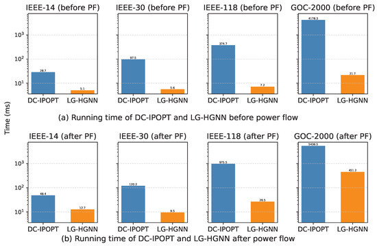
Figure 3. Average computational time (in ms) per instance comparing DC-IPOPT with LG-HGNN across different power systems.

In contrast, LG-HGNN maintains low inference latency, requiring only 5–7 ms for the 14- and 30-bus grids and below 30 ms for the 118-bus and 2000 cases before PF, since each prediction involves a fixed number of message-passing and attention layers. Consequently, LG-HGNN achieves substantial speed-ups of $\sim 6\times$, $\sim 18\times$, $\sim 52\times$, and $\sim 193\times$ before PF, and $\sim 4\times$, $\sim 13\times$, $\sim 37\times$, and $\sim 12\times$ after PF on the 14-, 30-, 118-, and GOC-2000 systems, respectively. Notably, for the 2000-bus case, the post-PF runtime is dominated by the power-flow correction step, which reduces the overall speed-up compared with the pure feed-forward inference stage. These gains are achieved without sacrificing accuracy or physical feasibility, indicating that the model can serve as an efficient surrogate for computationally intensive AC-OPF solvers.

Overall, the results highlight that LG-HGNN combines high physical fidelity with excellent practical scalability, delivering AC-feasible, near-optimal solutions within milliseconds.

6. Discussion

This section discusses the implications of the proposed LG-HGNN framework, its relation to existing AC-OPF solvers, and its current limitations.

6.1. Interpretation of Results

The results indicate that combining heterogeneous graph modeling with local–global message passing improves both accuracy and robustness for learning-based AC-OPF. The bus-centric global Transformer enables the model to capture long-range electrical dependencies that are difficult to represent using purely local message passing, particularly for voltage angles and reactive power variables. At the same time, explicitly distinguishing buses, generators, loads, and shunts allows the model to better reflect the physical structure of power systems, contributing to improved generalization under operating conditions and topology variations.

6.2. Comparison with Existing Methods

Compared with classical optimization-based solvers, LG-HGNN offers substantially faster inference at the cost of exact optimality guarantees, making it suitable for near-real-time or large-scale evaluation scenarios. In contrast to non-graph neural networks, which are sensitive to topology changes, the proposed graph-based formulation provides stronger structural inductive bias. Compared with existing GNN-based OPF solvers that rely solely on deep local message passing, LG-HGNN achieves competitive performance with fewer layers by introducing a physically motivated, bus-centric global aggregation mechanism, improving scalability and training stability.

6.3. Practical Implications and Limitations

LG-HGNN is best viewed as a fast surrogate or complementary tool to conventional AC-OPF solvers, for applications such as contingency screening, warm-start initialization, and large-scale scenario analysis. However, the approach depends on supervised training data and therefore inherits the limitations of available labeled AC-OPF datasets. In addition, while bounded decoders and physics-informed regularization reduce constraint violations, strict feasibility cannot be guaranteed without post-processing. Extending the framework to more complex OPF variants and hybrid learning–optimization pipelines remains an important direction for future work. Although the global attention module is restricted to bus nodes to reduce complexity, vanilla full attention over all bus nodes still scales quadratically with the number of buses in the worst case. For ultra-large grids (e.g., $|N_{bus}|>{10}^4$), this component may limit scalability and become a computational bottleneck. Exploring sparse- or linear-attention variants could further improve scalability, which we leave as future work.

7. Conclusions

This work introduces the Heterogeneous Graph Neural Network with Local–Global Message Passing (LG-HGNN) as an efficient surrogate for AC Optimal Power Flow (AC-OPF) in large-scale power networks. By explicitly modeling buses, generators, loads, and shunts as distinct node types and transmission lines, transformers, and connector edges as distinct relation types, LG-HGNN faithfully captures the physical heterogeneity of power systems. A bus-centric local–global architecture, which combines edge-aware heterogeneous message passing over the full graph with an effective-resistance-biased global Transformer operating only on bus nodes, enables the model to learn both local electrical interactions and long-range dependencies that are essential for AC power flow. Type-specific bounded decoders and physics-informed regularization further enforce operational limits and approximate power-balance constraints already during training.

Experiments on IEEE 14-, 30-, 118-bus and GOC 2000-bus systems from the OPFData benchmark show that LG-HGNN attains low prediction errors on bus, generator, and branch variables and yields operating points whose objective values are typically within a few percent of the AC-OPF optimum. When evaluated in a zero-shot setting on thousands of unseen N-1 contingency topologies, the model maintains competitive optimality ratios and feasibility metrics without topology-specific retraining, demonstrating strong topology-robust generalization. In terms of computational performance, LG-HGNN offers substantial speedups compared with conventional interior-point-based solvers and achieves up to around $190\times$ acceleration before AC power-flow post-processing and more than $10\times$ speedup even when a corrective power-flow step is applied, making it a promising candidate for near-real-time OPF applications in large-scale networks.

Despite its strong empirical performance, LG-HGNN may still exhibit small residual constraint violations and does not provide strict feasibility guarantees. An interesting direction for future work is to couple the proposed architecture with differentiable optimization layers or projection operators that can enforce feasibility certificates by design. Further extensions to incorporate uncertainty, dynamic operating conditions, and security-constrained OPF formulations, as well as to integrate hybrid learning–optimization schemes, are expected to enhance the reliability and applicability of learning-based AC-OPF surrogates in real-world power system operations.

References

- Cain, M.B.; O’neill, R.P.; Castillo, A. History of optimal power flow and formulations. Fed. Energy Regul. Comm. 2012, 1, 1–36. [Google Scholar]
- Khaloie, H.; Dolanyi, M.; Toubeau, J.F.; Vallée, F. Review of machine learning techniques for optimal power flow. Appl. Energy 2025, 388, 125637. [Google Scholar] [CrossRef]
- Panciatici, P.; Bareux, G.; Wehenkel, L. Operating in the fog: Security management under uncertainty. IEEE Power Energy Mag. 2012, 10, 40–49. [Google Scholar] [CrossRef]
- Hamann, H.F.; Gjorgiev, B.; Brunschwiler, T.; Martins, L.S.; Puech, A.; Varbella, A.; Weiss, J.; Bernabe-Moreno, J.; Massé, A.B.; Choi, S.L.; et al. Foundation models for the electric power grid. Joule 2024, 8, 3245–3258. [Google Scholar] [CrossRef]
- Shin, S.; Anitescu, M.; Pacaud, F. Accelerating optimal power flow with GPUs: SIMD abstraction of nonlinear programs and condensed-space interior-point methods. Electr. Power Syst. Res. 2024, 236, 110651. [Google Scholar] [CrossRef]
- Pan, X.; Chen, M.; Zhao, T.; Low, S.H. DeepOPF: A feasibility-optimized deep neural network approach for AC optimal power flow problems. IEEE Syst. J. 2022, 17, 673–683. [Google Scholar] [CrossRef]
- Yang, Z.; Zhong, H.; Bose, A.; Zheng, T.; Xia, Q.; Kang, C. A linearized OPF model with reactive power and voltage magnitude: A pathway to improve the MW-only DC OPF. IEEE Trans. Power Syst. 2017, 33, 1734–1745. [Google Scholar] [CrossRef]
- Molzahn, D.K.; Holzer, J.T.; Lesieutre, B.C.; DeMarco, C.L. Implementation of a large-scale optimal power flow solver based on semidefinite programming. IEEE Trans. Power Syst. 2013, 28, 3987–3998. [Google Scholar] [CrossRef]
- Chatzos, M.; Fioretto, F.; Mak, T.W.; Van Hentenryck, P. High-fidelity machine learning approximations of large-scale optimal power flow. arXiv 2020, arXiv:2006.16356. [Google Scholar]
- Baker, K. Solutions of DC OPF are never AC feasible. In Proceedings of the Twelfth ACM International Conference on Future Energy Systems, Virtual, 28 June–2 July 2021; pp. 264–268. [Google Scholar]
- Sun, D.I.; Ashley, B.; Brewer, B.; Hughes, A.; Tinney, W.F. Optimal power flow by Newton approach. IEEE Trans. Power Appar. Syst. 2007, PAS-103, 2864–2880. [Google Scholar] [CrossRef]
- Momoh, J.A.; Zhu, J. Improved interior point method for OPF problems. IEEE Trans. Power Syst. 1999, 14, 1114–1120. [Google Scholar] [CrossRef]
- Naderi, E.; Pourakbari-Kasmaei, M.; Abdi, H. An efficient particle swarm optimization algorithm to solve optimal power flow problem integrated with FACTS devices. Appl. Soft Comput. 2019, 80, 243–262. [Google Scholar] [CrossRef]
- Bian, J.; Wang, H.; Wang, L.; Li, G.; Wang, Z. Probabilistic optimal power flow of an AC/DC system with a multiport current flow controller. Csee J. Power Energy Syst. 2020, 7, 744–752. [Google Scholar]
- Abdulrasool, A.Q.; Al-Bahrani, L.T. Multi-objective constrained optimal power flow based on enhanced ant colony system algorithm. In Proceedings of the 2021 12th International Symposium on Advanced Topics in Electrical Engineering (ATEE), Bucharest, Romania, 25–27 March 2021; pp. 1–5. [Google Scholar]
- Xiang, P.; Tianyu, Z.; Minghua, C. DeepOPF: Deep neural network for DC optimal power flow. In Proceedings of the 2019 IEEE International Conference on Communications, Control, and Computing Technologies for Smart Grids, Beijing, China, 21–23 October 2019; pp. 1–6. [Google Scholar]
- Pan, X. Deepopf: Deep neural networks for optimal power flow. In Proceedings of the 8th ACM International Conference on Systems for Energy-Efficient Buildings, Cities, and Transportation, Coimbra, Portugal, 17–18 November 2021; pp. 250–251. [Google Scholar]
- Yang, Y.; Yang, Z.; Yu, J.; Zhang, B.; Zhang, Y.; Yu, H. Fast calculation of probabilistic power flow: A model-based deep learning approach. IEEE Trans. Smart Grid 2019, 11, 2235–2244. [Google Scholar] [CrossRef]
- Owerko, D.; Gama, F.; Ribeiro, A. Optimal power flow using graph neural networks. In Proceedings of the ICASSP 2020–2020 IEEE International Conference on Acoustics, Speech and Signal Processing (ICASSP), Barcelona, Spain, 4–8 May 2020; pp. 5930–5934. [Google Scholar]
- Falconer, T.; Mones, L. Leveraging power grid topology in machine learning assisted optimal power flow. IEEE Trans. Power Syst. 2022, 38, 2234–2246. [Google Scholar] [CrossRef]
- Liu, S.; Wu, C.; Zhu, H. Topology-aware graph neural networks for learning feasible and adaptive AC-OPF solutions. IEEE Trans. Power Syst. 2022, 38, 5660–5670. [Google Scholar] [CrossRef]
- Piloto, L.; Liguori, S.; Madjiheurem, S.; Zgubic, M.; Lovett, S.; Tomlinson, H.; Elster, S.; Apps, C.; Witherspoon, S. Canos: A fast and scalable neural ac-opf solver robust to n-1 perturbations. arXiv 2024, arXiv:2403.17660. [Google Scholar] [CrossRef]
- Gao, M.; Yu, J.; Yang, Z.; Zhao, J. A physics-guided graph convolution neural network for optimal power flow. IEEE Trans. Power Syst. 2023, 39, 380–390. [Google Scholar] [CrossRef]
- Veličković, P.; Cucurull, G.; Casanova, A.; Romero, A.; Lio, P.; Bengio, Y. Graph attention networks. arXiv 2017, arXiv:1710.10903. [Google Scholar]
- Xu, K.; Hu, W.; Leskovec, J.; Jegelka, S. How powerful are graph neural networks? arXiv 2018, arXiv:1810.00826. [Google Scholar]
- Ahmad, N.; Ghadi, Y.; Adnan, M.; Ali, M. Load forecasting techniques for power system: Research challenges and survey. IEEE Access 2022, 10, 71054–71090. [Google Scholar] [CrossRef]
- Omar, M.; Sayed, E.; Abdalmagid, M.; Bilgin, B.; Bakr, M.H.; Emadi, A. Review of machine learning applications to the modeling and design optimization of switched reluctance motors. IEEE Access 2022, 10, 130444–130468. [Google Scholar] [CrossRef]
- Chowdhury, M.M.U.T.; Kamalasadan, S.; Paudyal, S. A second-order cone programming (socp) based optimal power flow (opf) model with cyclic constraints for power transmission systems. IEEE Trans. Power Syst. 2023, 39, 1032–1043. [Google Scholar] [CrossRef]
- Chowdhury, M.M.U.T.; Hasan, M.S.; Kamalasadan, S. A distributed optimal power flow (d-opf) model for radial distribution networks with second-order cone programming (socp). In Proceedings of the 2023 IEEE Industry Applications Society Annual Meeting (IAS), Nashville, TN, USA, 29 October–2 November 2023; pp. 1–8. [Google Scholar]
- Sasson, A.M. Combined use of the Powell and Fletcher-Powell nonlinear programming methods for optimal load flows. IEEE Trans. Power Appar. Syst. 2007, PAS-88, 1530–1537. [Google Scholar] [CrossRef]
- Lavaei, J.; Low, S.H. Convexification of optimal power flow problem. In Proceedings of the 2010 48th Annual Allerton Conference on Communication, Control, and Computing (Allerton), Monticello, IL, USA, 29 September–1 October 2010; pp. 223–232. [Google Scholar]
- Low, S.H. Convex relaxation of optimal power flow—Part II: Exactness. IEEE Trans. Control Netw. Syst. 2014, 1, 177–189. [Google Scholar] [CrossRef]
- Kile, H.; Uhlen, K.; Warland, L.; Kjølle, G. A comparison of AC and DC power flow models for contingency and reliability analysis. In Proceedings of the 2014 Power Systems Computation Conference, Wroclaw, Poland, 18–22 August 2014; pp. 1–7. [Google Scholar]
- Torres, G.L.; Quintana, V.H. An interior-point method for nonlinear optimal power flow using voltage rectangular coordinates. IEEE Trans. Power Syst. 2002, 13, 1211–1218. [Google Scholar] [CrossRef]
- Roa-Sepulveda, C.; Pavez-Lazo, B. A solution to the optimal power flow using simulated annealing. Int. J. Electr. Power & Energy Syst. 2003, 25, 47–57. [Google Scholar]
- Velloso, A.; Van Hentenryck, P. Combining deep learning and optimization for preventive security-constrained DC optimal power flow. IEEE Trans. Power Syst. 2021, 36, 3618–3628. [Google Scholar] [CrossRef]
- Park, S.; Chen, W.; Mak, T.W.; Van Hentenryck, P. Compact optimization learning for AC optimal power flow. IEEE Trans. Power Syst. 2023, 39, 4350–4359. [Google Scholar] [CrossRef]
- Huang, W.; Chen, M.; Low, S.H. Unsupervised learning for solving AC optimal power flows: Design, analysis, and experiment. IEEE Trans. Power Syst. 2024, 39, 7102–7114. [Google Scholar] [CrossRef]
- Jia, Y.; Bai, X.; Zheng, L.; Weng, Z.; Li, Y. ConvOPF-DOP: A data-driven method for solving AC-OPF based on CNN considering different operation patterns. IEEE Trans. Power Syst. 2022, 38, 853–860. [Google Scholar] [CrossRef]
- Zamzam, A.S.; Baker, K. Learning optimal solutions for extremely fast AC optimal power flow. In Proceedings of the 2020 IEEE International Conference on Communications, Control, and Computing Technologies for Smart Grids (SmartGridComm), Tempe, AZ, USA, 11–13 November 2020; pp. 1–6. [Google Scholar]
- Chatzos, M.; Mak, T.W.; Van Hentenryck, P. Spatial network decomposition for fast and scalable AC-OPF learning. IEEE Trans. Power Syst. 2021, 37, 2601–2612. [Google Scholar] [CrossRef]
- Scarselli, F.; Gori, M.; Tsoi, A.C.; Hagenbuchner, M.; Monfardini, G. The graph neural network model. IEEE Trans. Neural Netw. 2008, 20, 61–80. [Google Scholar] [CrossRef] [PubMed]
- Donon, B.; Clément, R.; Donnot, B.; Marot, A.; Guyon, I.; Schoenauer, M. Neural networks for power flow: Graph neural solver. Electr. Power Syst. Res. 2020, 189, 106547. [Google Scholar] [CrossRef]
- Zhou, M.; Chen, M.; Low, S.H. DeepOPF-FT: One deep neural network for multiple AC-OPF problems with flexible topology. IEEE Trans. Power Syst. 2022, 38, 964–967. [Google Scholar] [CrossRef]
- Babaeinejadsarookolaee, S.; Birchfield, A.; Christie, R.D.; Coffrin, C.; DeMarco, C.; Diao, R.; Ferris, M.; Fliscounakis, S.; Greene, S.; Huang, R.; et al. The power grid library for benchmarking ac optimal power flow algorithms. arXiv 2019, arXiv:1908.02788. [Google Scholar]
- Lovett, S.; Zgubic, M.; Liguori, S.; Madjiheurem, S.; Tomlinson, H.; Elster, S.; Apps, C.; Witherspoon, S.; Piloto, L. OPFData: Large-scale datasets for AC optimal power flow with topological perturbations. arXiv 2024, arXiv:2406.07234. [Google Scholar] [CrossRef]
- Yehudai, G.; Fetaya, E.; Meirom, E.; Chechik, G.; Maron, H. From local structures to size generalization in graph neural networks. In Proceedings of the International Conference on Machine Learning, Virtual, 18–24 July 2021; pp. 11975–11986. [Google Scholar]
- Rampášek, L.; Galkin, M.; Dwivedi, V.P.; Luu, A.T.; Wolf, G.; Beaini, D. Recipe for a general, powerful, scalable graph transformer. Adv. Neural Inf. Process. Syst. 2022, 35, 14501–14515. [Google Scholar]
- Raissi, M.; Perdikaris, P.; Karniadakis, G.E. Physics-informed neural networks: A deep learning framework for solving forward and inverse problems involving nonlinear partial differential equations. J. Comput. Phys. 2019, 378, 686–707. [Google Scholar] [CrossRef]
- Lu, L.; Pestourie, R.; Yao, W.; Wang, Z.; Verdugo, F.; Johnson, S.G. Physics-informed neural networks with hard constraints for inverse design. SIAM J. Sci. Comput. 2021, 43, B1105–B1132. [Google Scholar] [CrossRef]
- Varbella, A.; Briens, D.; Gjorgiev, B.; D’Inverno, G.A.; Sansavini, G. Physics-Informed GNN for non-linear constrained optimization: PINCO a solver for the AC-optimal power flow. arXiv 2024, arXiv:2410.04818. [Google Scholar]
- Fioretto, F.; Mak, T.W.; Van Hentenryck, P. Predicting ac optimal power flows: Combining deep learning and lagrangian dual methods. Proc. Aaai Conf. Artif. Intell. 2020, 34, 630–637. [Google Scholar] [CrossRef]
- Baker, K. Learning warm-start points for AC optimal power flow. In Proceedings of the 2019 IEEE 29th International Workshop on Machine Learning for Signal Processing (MLSP), Pittsburgh, PA, USA, 13–16 October 2019; pp. 1–6. [Google Scholar]
- Crozier, C.; Baker, K. Data-driven probabilistic constraint elimination for accelerated optimal power flow. In Proceedings of the 2022 IEEE Power & Energy Society General Meeting (PESGM), Denver, CO, USA, 17–21 July 2022; pp. 1–5. [Google Scholar]
- Cetinay, H.; Kuipers, F.A.; Van Mieghem, P. A topological investigation of power flow. IEEE Syst. J. 2016, 12, 2524–2532. [Google Scholar] [CrossRef]
Disclaimer/Publisher’s Note: The statements, opinions and data contained in all publications are solely those of the individual author(s) and contributor(s) and not of MDPI and/or the editor(s). MDPI and/or the editor(s) disclaim responsibility for any injury to people or property resulting from any ideas, methods, instructions or products referred to in the content. |
© 2026 by the authors. Published by MDPI on behalf of the International Institute of Knowledge Innovation and Invention. Licensee MDPI, Basel, Switzerland. This article is an open access article distributed under the terms and conditions of the Creative Commons Attribution (CC BY) license.