Optimization of Crowbar Resistance for Enhanced LVRT Capability in Wind Turbine Doubly Fed Induction Generator

Abstract

Recently, the installed generation capacity of wind energy has expanded significantly, and the doubly fed induction generator (DFIG) has gained a prominent position amongst wind generators owing to its superior performance. It is extremely vital to enhance the low-voltage ride-through (LVRT) capability for the wind turbine DFIG system because the DFIG is very sensitive to faults in the electrical grid. The major concept of LVRT is to keep the DFIG connected to the electrical grid in the case of an occurrence of grid voltage sags. The currents of rotor and DC-bus voltage rise during voltage dips, resulting in damage to the power electronic converters and the windings of the rotor. There are many protection approaches that deal with LVRT capability for the wind turbine DFIG system. A popular approach for DFIG protection is the crowbar technique. The resistance of the crowbar must be precisely chosen owing to its impact on both the currents of the rotor and DC-bus voltage, while also ensuring that the rotor speed does not exceed its maximum limit. Therefore, this paper aims to obtain the optimal values of crowbar resistance to minimize the crowbar energy losses and ensure stable DFIG operation during grid voltage dips. A recent optimization technique, the Starfish Optimization (SFO) algorithm, was used for cropping the optimal crowbar resistance for improving LVRT capability. To validate the accuracy of the results, the SFO results were compared to the well-known optimization algorithm, particle swarm optimizer (PSO). The performance of the wind turbine DFIG system was investigated by using Matlab/Simulink at a rated wind speed of 13 m/s. The results demonstrated that the increases in DC-link voltage and rotor speed were reduced by 42.5% and 45.8%, respectively.

1. Introduction

The escalation of international power consumption and energy demand is attributable to industrial expansion and societal development. However, owing to the constraints of fossil fuel supplies and their environmental repercussions, solar, wind, and hydro energy are regarded as the most significant sources of renewable energy; their technologies are developing dramatically. Wind energy is a clean, renewable energy source that produces no greenhouse gas emissions. It is the second most widely used renewable energy source after hydropower [1,2,3]. A common configuration for large variable-speed wind systems is a doubly fed induction generator (DFIG), in which the windings of the rotor act as a power interface between the grid and the rotor windings via a back-to-back converter, while the windings of the stator are directly connected to the grid. Significant reasons that make the DFIG more popular in wind systems are that the rating of the power electronic converter is in the range of 25 to 30% of the system power, and the system can operate over a wide range of speeds. The rotor-side converter (RSC) can adjust both reactive and real powers independently. Meanwhile, DC-bus voltage can be adjusted by the grid-side converter (GSC), providing the reactive power exchange to the grid [4,5,6].

Due to the direct connection between the stator of DFIG and the electrical grid, DFIG is extremely sensitive to the faults of the grid. A dip in the voltage of the grid generates a disturbance in the current and voltage of the stator, resulting in high voltage and current at the side of the rotor, leading to damage to the back-to-back converter and the windings of the rotor. In accordance with contemporary grid code, as depicted in Figure 1, wind turbines must remain connected to the electrical grid in the event of a voltage sag, which is called a low-voltage ride-through (LVRT) or fault ride-through (FRT), which has been defined by different grid codes depending on the country [7,8,9]. There are several strategies for dealing with the issue of LVRT. The basic concept of the first category is the usage of power electronics devices such as the dynamic voltage restorer (DVR), static VAR compensator (SVC), crowbars (CB), unified power flow controller (UPFC), static synchronous compensator (STATCOM), and braking chopper. The second category is based on the connection between energy storage systems (ESSs) and power electronics switches. The third group depends on complex control methods like predictive control, pitch angle control, and vector control methods. In contrast, the DFIG control-based LVRT techniques are incapable of providing proper responses during high dips in the grid voltage [7,8,10,11,12,13,14].

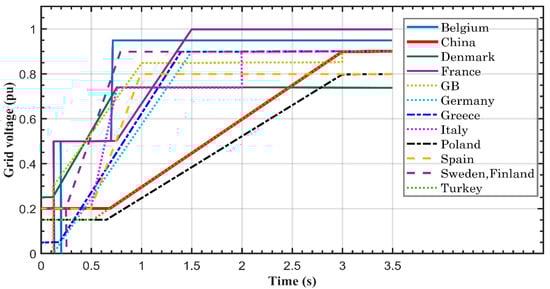
Figure 1. LVRT requirements as defined by the TSOs of different countries [9].

The crowbar protection method is the most predominant hardware option for DFIG-based LVRT. It is composed of three switches with three resistors, or a rectifier with one resistor, which are added to the circuit of the rotor. The activation and release of the crowbar circuit and the current controller of the rotor-side converter are the two basic means to perform the LVRT of DFIG. When the crowbar circuit is inserted into the rotor of DFIG, the back-to-back converter and wind turbine become uncontrolled. Therefore, the controllers of converters reactivate only after releasing the crowbar circuit. The DFIG becomes a squirrel cage induction generator by inserting the circuit of a crowbar, leading to protecting the rotor-side converter and limiting the rotor current [15]. The crowbar resistance value is crucial in influencing the performance of DFIG during LVRT, as it directly affects the rotational speed, rotor currents, DC-bus voltage, and both reactive and real power. Thus, it is important to carefully determine the crowbar resistance value, where the selection of an appropriate resistance value necessitates balancing two conflicting requirements [16,17,18]. On one hand, the crowbar resistance value must be sufficiently high to limit high rotor currents during grid voltage dips, which could damage the rotor windings. On the other hand, high crowbar resistance leads to unstable operation of DFIG, such as exceeding the DFIG speed above the maximum allowable speed and causing high DC-bus voltage [19,20,21,22].

The contribution of this paper is obtaining the optimal crowbar resistance that achieves three objectives at different values of grid voltage dips. The first objective is the minimization of the DFIG speed to not exceed the maximum allowable speed, and the second objective is to reduce the energy losses of the crowbar circuit. In contrast, the third objective is to minimize the DFIG speed and the energy losses of the crowbar circuit. A new optimization algorithm, the Starfish Optimization (SFO) algorithm, which was developed in 2025, was employed to obtain the optimal value of crowbar resistance with the aim of achieving the three objectives. The remainder of this paper is structured as follows. Section 2 presents the materials and methods, including an overview of the wind turbine DFIG model with crowbar protection, a description of the SFO, and the crowbar resistance optimization procedure. Section 3 provides the simulation results. Section 4 discusses and interprets these results. Finally, the conclusions are presented in Section 5.

2. Materials and Methods

2.1. DFIG Modeling with Crowbar Protection

The basic components of the wind turbine DFIG system with the crowbar protection method are the wind turbine, DFIG, back-to-back power converters, RSC, and GSC, and their controllers, as shown in Figure 2. Crowbar protection is put into operation when the rotor overcurrent exceeds the rated capacity of the converter by two times, which is caused by a power grid voltage dip. At the same time, the rotor-side converter (RSC) is blocked, and the impact of large current in the rotor winding is rapidly consumed and attenuated because of the crowbar resistance, so that the RSC and the grid-side converter (GSC) are protected from flowing impact current [23,24,25].

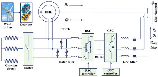
Figure 2. The wind turbine DFIG system with a crowbar protection circuit.

2.1.1. Wind Turbine Model

The wind kinetic energy is transformed by a wind turbine into mechanical energy, which rotates the wind turbine blades that are coupled to a low-speed shaft. Then, a gearbox is used to transmit the mechanical energy into a high-speed shaft for the generation of electrical power by a DFIG. The variable pitch angle turbine can harvest the maximum available wind power by raising or lowering the pitch angle of the wind turbine blades in accordance with the amount of energy produced. The modeling of a wind turbine can be performed by the following equations [26,27,28].

$$P_{TURBINE}={\displaystyle \frac{1}{2}} \pi \rho R_b^2 V_{WIND}^3 {Co}_P\left(\beta ,\gamma \right)$$

(1)

$$T_{TURBINE}={\displaystyle \frac{P_{TURBINE}}{{\omega }_t}}$$

(2)

$${Co}_P=0.73 \left( {\displaystyle \frac{151}{{\gamma }_i}}-0.58 \beta -0.002 {\beta }^{2.14}-13.2\right)e^{{\displaystyle \frac{-18.4}{{\gamma }_i}}}$$

(3)

$${\displaystyle \frac{1}{{\gamma }_i}}={\displaystyle \frac{1}{\gamma +0.02\beta }}-{\displaystyle \frac{0.003}{{\beta }^3+1}}$$

(4)

$$\gamma ={\displaystyle \frac{{\omega }_{TURBINE} R_b}{V_{WIND}}}$$

(5)

where, $P_{Turbine}$ and $T_{Turbine}$ are the power and torque of a wind turbine; $V_{WIND}$ is the wind speed (m/s); ${\omega }_{TURBINE}$ is the rotational speed of the wind turbine (rad/s); $\rho$ is the density of air (kg/m³); and $R_b$ is the wind turbine blades’ radius. The power conversion coefficient of a wind turbine $\left({Co}_P\right)$ can be determined by Equation (3) based on the pitch angle $\beta$ (degree) and the tip speed ratio $\left(\gamma \right)$ [29].

Figure 3 shows the ideal curve of a wind turbine that is vital in choosing an appropriate control type for a wind turbine for improvement in the efficiency and quality of power conversion. The range of operating wind speeds is between the cut-in wind speed and the cut-out wind speed. There are four operating regions in which a wind turbine may operate in these regions, as shown in Figure 3 [30,31]. A wind turbine is operated in region 1 if the wind speed is below the cut-in speed. In this region, the turbine is set to be turned off because the available wind power is too low to compensate for the turbine blades’ friction for rotating the blades. When the wind speed is between the cut-in and rated speeds, a wind turbine is operated in region 2.

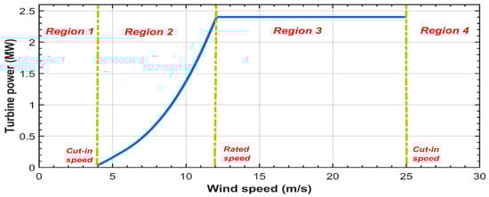
Figure 3. Wind turbine ideal power curve and its operation modes.

In this region, the maximum available power can be tracked by adjusting the rotational wind turbine speed and setting the pitch angle to zero. In comparison, a wind turbine is operated in region 3 if the wind speed is above the rated wind speed and below the cut-out wind speed. In this region, the output power of the turbine can be restricted or controlled by the activation of the controller of the pitch angle. When the wind speed is above the cut-out wind speed, a turbine is operated in region 4. In this region, the braking mechanism is activated to turn off the turbine because the turbine and generator will be damaged at any speed above the cut-out speed [31,32,33,34].

2.1.2. Dynamic Modeling of DFIG

DFIG dynamic modeling is required for dynamic analysis and designing the control system. The DFIG is a time-varying, non-linear, high-order system. For developing the dynamic model of DFIG, there are some assumptions: the unsaturated magnetic circuit of the DFIG; the stator and rotor currents and voltages are determined in the positive direction as the motor; and all the electric quantities of the rotor circuit have been referred to the stator side. The DQ dynamic model, which is based on the idea of the theory of classical rotating fields, can be used to study the DFIG operation concept. The dynamic DFIG equations based on the DQ equivalent model in the rotating synchronous DQ reference frame, as demonstrated in Figure 4, are given as follows [6,28,35,36,37,38,39,40].

$$V_{SD}=R_S i_{SD}-{\omega }_S {\psi }_{SQ}+{\displaystyle \frac{d}{dt}} {\psi }_{SD}$$

(6)

$$V_{SQ}=R_S i_{SQ}+{\omega }_S {\psi }_{SD}+{\displaystyle \frac{d}{dt}} {\psi }_{SQ}$$

(7)

$$V_{RD}=R_R i_{RD}-\left({\omega }_S-{\omega }_R\right) {\psi }_{RQ}+{\displaystyle \frac{d}{dt}} {\psi }_{RD}$$

(8)

$$V_{RQ}=R_R i_{RQ}+\left({\omega }_S-{\omega }_R\right) {\psi }_{RD}+{\displaystyle \frac{d}{dt}} {\psi }_{RQ}$$

(9)

$${\psi }_{SD}=L_S i_{SD}+L_M i_{RD}$$

(10)

$${\psi }_{SQ}=L_S i_{SQ}+L_M i_{RQ}$$

(11)

$${\psi }_{RD}=L_R i_{RD}+L_M i_{SD}$$

(12)

$${\psi }_{RQ}=L_R i_{RQ}+L_M i_{SQ}$$

(13)

$$P_{Stator}=1.5 \left(V_{SD} i_{SD}+V_{SQ} i_{SQ}\right)$$

(14)

$$Q_{Stator}=1.5 \left(V_{SQ} i_{SD}-V_{SD} i_{SQ}\right)$$

(15)

$$P_{Rotor}=1.5 \left(V_{RD} i_{RD}+V_{RQ}{ i}_{RQ}\right)$$

(16)

$$Q_{Rotor}=1.5 \left(V_{RQ} i_{RD}-V_{RD} i_{RQ}\right)$$

(17)

where $V_{SD}$, $V_{SQ}$, $V_{RD}$, and $V_{RQ}$ are the D and Q components of the stator and rotor voltages; $i_{SD}$, $i_{SQ}$, $i_{RD}$, and $i_{RQ}$ are the D and Q components of the stator and rotor currents. ${\omega }_S$ and ${\omega }_R$ are the current and voltage frequencies for the stator and rotor (rad/s). $R_S$ and $R_R$ are the resistance of the stator and rotor winding. ${\psi }_{SD}$, ${\psi }_{SQ}$, ${\psi }_{RD}$, and ${\psi }_{RQ}$ are the D and Q components of the stator and rotor flux. $L_S$, $L_R$, and $L_M$ are the stator and rotor and mutual inductances. $P_{Stator}$, $P_{Rotor}$, $Q_{Stator}$, and $Q_{Rotor}$ are the active and reactive powers of the stator and rotor. The DFIG electromagnetic torque ($T_{EM}$) and the mechanical torque generated by a wind turbine ($T_M$) are given as follows:

$$T_{EM}= {\displaystyle \frac{3 p }{2 }} {\displaystyle \frac{ L_M}{L_S}} \left({\psi }_{SQ} i_{RD}- {\psi }_{SD} i_{RQ}\right)$$

(18)

$$T_M-T_{EM}=J{\displaystyle \frac{d{\mathsf{\omega }}_m}{dt}}+f {\mathsf{\omega }}_m$$

(19)

where $J$ is the total inertia (kg.m²); $p$ is the pole pairs; $f$ is the friction factor (N.m.s); ${\mathsf{\omega }}_m$ is the mechanical shaft speed (rad/s).

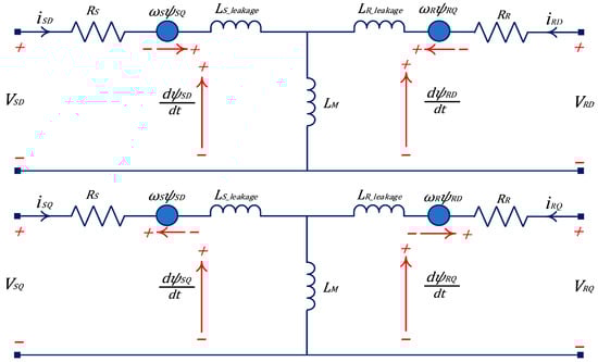
Figure 4. The DFIG dynamic model based on the DQ reference frame.

2.2. Starfish Optimization Algorithm

The SFO is an innovative biologically inspired method for addressing optimization challenges, emulating starfish behaviors such as predation, exploration, and regeneration. It comprises two primary stages: exploration as well as exploitation. The stage of exploration emulates the exploratory behavior of starfish through a hybrid search pattern that combines the five-unidimensional and dimensional search patterns in order to boost the computing efficiency and guarantee the capacity of search. In comparison, the stage of exploitation emulates the regeneration and predation behaviors of starfish through a two-directional search approach and unique motion in order to achieve convergence in the exploitation. The SFO flowchart is shown in Figure 5 to clearly illustrate the process. The procedure of SFO can be summarized as follows [41,42,43]. For the phase of initialization, the population is randomly generated within the design variable boundaries using Equation (20) after the input SFO parameters and the optimization problem are defined. The values of fitness for all starfish are then evaluated and stored as a vector. Every starfish position in Equation (20) is assessed by Equation (21).

$$x=\left[\begin{array}{ccc}\begin{array}{c}{x}_{11}\\ x_{21}\\ \begin{array}{c}⋮\\ x_{n1}\end{array}\end{array}& \begin{array}{c}{x}_{12}\\ x_{22}\\ \begin{array}{c}⋮\\ x_{n2}\end{array}\end{array}& \begin{array}{cc}\begin{array}{c}\dots \\ \dots \\ \begin{array}{c}\ddots \\ \dots \end{array}\end{array}& \begin{array}{c}{x}_{1d}\\ x_{2d}\\ \begin{array}{c}⋮\\ x_{nd}\end{array}\end{array}\end{array}\end{array}\right]\begin{array}{c}R\\ N\\ \begin{array}{c}N\\ \begin{array}{c}N\\ n\times d\end{array}\end{array}\end{array}$$

(20)

$$x_{ij}={lb}_j+r\left({ub}_j-{lb}_j\right), i=\mathrm{1,2},\dots ,n, j=\mathrm{1,2},\dots ,d$$

(21)

where $x$ is the matrix for storing the starfish positions; $d$ is the design variables’ dimension; $n$ is the size of the population; $x_{ij}$ is the jth dimension position of the ith starfish; ${ub}_j$ and ${lb}_j$ are the lower and upper bounds of the design variables for the jth dimension position, respectively; $r$ is the random number between zero and one.

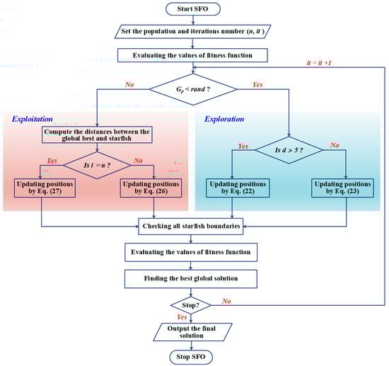
Figure 5. The flowchart of SFO.

Following the initialization stage, SFO moves into the core loop and begins the phases of exploration and exploitation. The exploitation and exploration stages have a similar probability of being implemented according to the comparison between the algorithmic parameter ($G_p$) equaling 0.5 and a random number ($rand$) between zero and one. For the stage of exploration, a hybrid search technique is adopted, incorporating both five-unidimensional and dimensional search patterns. There are two approaches to updating the starfish positions for various dimensions. If the dimension of design variables for the problem of optimization is less than five, Equation (22) is used to update the starfish position. If this condition is not achieved, it is updated by Equation (23). Then, after the starfish positions have been updated, Equation (24) is employed to verify the design variables’ boundaries [41,42,43].

$$\left\{\begin{array}{c}{y_{i,P}^{it}=x}_{i,P}^{it}+\pi (2r-1) \left(x_{best,P}^{it}-x_{i,P}^{it}\right) \mathrm{c}\mathrm{o}\mathrm{s}( {\displaystyle \frac{\pi }{2}} {\displaystyle \frac{it}{{it}_{max}}} ), r\le 0.5\\ {y_{i,P}^{it}=x}_{i,P}^{it}-\pi (2r-1) \left(x_{best,P}^{it}-x_{i,P}^{it}\right) \mathrm{s}\mathrm{i}\mathrm{n}( {\displaystyle \frac{\pi }{2}} {\displaystyle \frac{it}{{it}_{max}}} ), r>0.5\end{array}\right.$$

(22)

$$y_{i,q}^{it}=\left({\displaystyle \frac{{it}_{max}-it}{{it}_{max}}} \mathrm{c}\mathrm{o}\mathrm{s}({\displaystyle \frac{\pi }{2}} {\displaystyle \frac{it}{T_{max}}})\right) x_{i,P}^{it}+A_1\left(x_{k1,P}^{it}-x_{i,P}^{it}\right)+A_2\left(x_{k2,P}^{it}-x_{i,P}^{it}\right)$$

(23)

$$x_{i,P}^{it+1}=\left\{\begin{array}{c}{y}_{i,P}^{it} {lb}_P\le y_{i,P}^{it}\le {ub}_P\\ x_{i,P}^{it} otherwise\end{array}\right.$$

(24)

where $x_{i,P}^{it}$ and $y_{i,P}^{it}$ are the current and obtained starfish positions, respectively. $P$ is the selected random number in the d dimensions. $x_{best,P}^{it}$ is the P-dimension of the best current position. $it$ and ${it}_{max}$ are the current and maximum iteration. $x_{k1,P}^{it}$ and $x_{k2,P}^{it}$ are the P-dimensional positions from two selected random starfish. $A_1$ and $A_2$ are two random numbers between −1 and 1. For the stage of exploitation, Equation (25) is employed to calculate the distances between the global solution and other starfish based on the two-directional parallel search pattern. After that, SFO updates every starfish position by using the behavior of preying according to Equation (26). Then, the stage of regeneration occurs when the order of starfish position equals the size of the population, and its position is updated by Equation (27). Once the starfish positions have been updated in the stage of exploitation, Equation (28) is employed to verify the design variables’ boundaries. If the obtained starfish position from Equation (26) or Equation (27) is out of the limits of design variables, Equation (28) is used to set the position [41,42,43].

$$d_m=\left(x_{best}^{it}-x_{m_P}^{it}\right), m=1,\dots ,5$$

(25)

$$y_i^{it}=x_i^{it}+r_1 d_{m1}+r_2 d_{m2}$$

(26)

$$y_i^{it}=\exp \left(-it\times N/{it}_{max}\right)x_i^{it}$$

(27)

$$x_i^{it+1}=\left\{\begin{array}{c}{y}_i^{it} lb \le y_i^{it} \le ub\\ \begin{array}{c}lb y_i^{it}<lb\\ ub y_i^{it}>ub\end{array}\end{array}\right.$$

(28)

where $d_m$ are the obtained five distances between the best global starfish and other starfish. $m_p$ are five selected random starfish. $r_1$ and $r_2$ are random numbers between zero and one. $d_{m1}$ and $d_{m2}$ are selected random numbers in $d_m$. Finally, the fitness values are computed following the update of starfish positions from every stage. The stopping condition is determined by the maximum iteration where SFO outputs the global solution and the curve of convergence.

2.3. Crowbar Resistance Optimization

The optimal resistance of the crowbar circuit ($R_{\mathrm{C}\mathrm{r}\mathrm{o}\mathrm{w}\mathrm{b}\mathrm{a}\mathrm{r}}$) is obtained by two optimization methods, SFO and PSO, to achieve three objective goals. When the grid voltage dips, the speed of DFIG may increase above the maximum allowable speed (1900 rpm), and the rotor currents increase above the rated rotor current. Therefore, it is necessary to minimize the maximum DFIG speed and the rotor currents during the grid voltage sag. Three optimization function objectives are taken to achieve different goals to enhance LVRT capability.

The first objective of the optimization function (${Obj}_1$) is minimizing the maximum DFIG speed during the period of grid voltage dip with the constraints that the rotor currents do not exceed 1.2 times the rated rotor current and that the DFIG speed does not exceed the maximum allowable speed, as illustrated in Equation (29). The optimization function is achieved by the variation of one input variable, which is the crowbar resistance.

$${Obj}_1=Minimize\left(N_{Max\_DFIG}\right) \mathrm{with} \mathrm{constraints} \left\{\begin{array}{c}{N}_{Max\_DFIG}\le 1900\\ I_{Max\_R}\le 1.2 I_{R_{rated}}\end{array}\right.$$

(29)

where, $N_{Max\_DFIG}$ is the maximum DFIG speed during a voltage dip. $I_{\mathrm{M}\mathrm{a}\mathrm{x}\_\mathrm{R}}$ is the maximum rotor current during a voltage dip. $I_{R_{rated}}$ is the rated value of rotor current.

The second objective of the optimization function (${Obj}_2$) is minimizing the crowbar energy losses ($E_{Crowbar}$) during the grid voltage dip period with the constraints that the rotor currents do not exceed 1.2 times the rated rotor current and that the DFIG speed does not exceed the maximum allowable speed, as illustrated in Equation (30). The optimization function is achieved by the variation of one input variable: the crowbar resistance.

$${Obj}_2=Minimize\left(E_{Crowbar}\right) \mathrm{with} \mathrm{constraints} \left\{\begin{array}{c}{N}_{Max\_DFIG}\le 1900\\ I_{Max\_R}\le {1.2 I}_{R_{rated}}\end{array}\right.$$

(30)

Meanwhile, the third objective of the optimization function (${Obj}_3$) is to minimize both the maximum DFIG speed and the crowbar energy losses (kJ) when the grid voltage dips, with the constraints that the rotor currents do not exceed 1.2 times the rated rotor current and that the DFIG speed does not exceed the maximum allowable speed, as illustrated in Equation (31). The optimization function is achieved by the variation of one input variable: the crowbar resistance.

$${Obj}_3=Minimize\left(abs\left(N_{Ma{x}_{DFIG}}-1900\right)+E_{Crowbar}\right) \mathrm{with} \mathrm{constraints} \left\{\begin{array}{c}{N}_{Max\_DFIG}\le 1900\\ I_{Max\_R}\le {1.2 I}_{R_{rated}}\end{array}\right.$$

(31)

3. Results

The Matlab/Simulink software (Release 12b.) was used to simulate the model of the wind turbine DFIG system with a crowbar protection circuit. Table 1 shows the wind turbine and DFIG parameters. Table 2 presents the gains of the PI controllers, which are used in RSC and GSC controllers, and DC-bus capacitance and its reference voltage. Figure 6 demonstrates the schematic diagram of a grid-connected DFIG wind turbine system with a crowbar protection circuit in Simulink. The system was studied at a 13 m/s wind speed and two cases of grid voltage dips: a 0.8 voltage dip (new voltage is 0.2 pu) and a 0.6 voltage dip (new voltage is 0.4 pu).

Table 1. The parameters of the wind turbine and DFIG [29].

Grid Data
Grid line voltage	690 V (rms)
Grid frequency	60 Hz
DFIG and wind turbine inertia	127 kg.m2
Friction factor	0.001 N.m.s
Wind turbine
Rated mechanical power	2.4 MW
Rotor diameter	42 m
Wind speed range	4–25 m/s
Rated wind speed	12.1 m/s
Gearbox ratio	100
Nominal rotor speed range	9–19 rpm
DFIG
Rated stator power	2 MW
Rated stator line voltage	690 V (rms)
Rated stator current	1760 A (rms)
Rated rotor current	1823 A (rms)
Rated rotor line voltage	845 V (rms)
Rated torque	12.732 kN.m
Rated rotor speed	1800 rpm
Rotor speed range	900–1900 rpm
Pole number	4
RS, RR	2.6, 2.9 m$\Omega$
LS, LR	87, 87 μH
LM	2.5 mH

Table 2. The data of controllers and filters for RSC and GSC [40].

Rotor L-C filter
CF, RF, LF	1493.1 μF, 1.09 $\Omega$, 3.57 mH
Grid L filter
Lg, Rg	0.2400 mH, 0.000115 $\Omega$
DC-bus voltage and capacitance
CDC-bus	395.0622 mF
VDC-bus	1306.11 V
PI controller gains for RSC Controller
The tracking of DFIG speed	$K_P=$ 6893.13, $K_i$ = 47,955.20
The tracking of D components of rotor currents	$K_P=$ 5.44, $K_i$ = 674.94
The tracking of Q components of rotor currents	$K_P=$ 6.18, $K_i$ = 647.87
PI controller gains for RSC Controller
The tracking of DC-bus voltage	$K_P=$ −3054.95, $K_i$ = −790,888.91
The tracking of D components of grid currents	$K_P=$ 1.41, $K_i$ = 404.47
The tracking of Q components of grid currents	$K_P=$ 60.05, $K_i$ = 1343.17

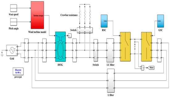
Figure 6. The Simulink model of the wind turbine DFIG system with a crowbar protection circuit.

Figure 7 demonstrates the crowbar energy losses at the 0.8 grid voltage dip for three objective functions based on SFO and PSO. Figure 8 shows the DFIG speed at the 0.8 grid voltage dip for three objective functions based on two optimization methods. As shown in Figure 7 and Figure 8, optimizing for energy losses only (${Obj}_2$) reduces the crowbar energy loss from 61.5 kJ to 25.1 kJ, whereas optimizing for maximum generator speed only (${Obj}_1$) limits the peak rotor speed during the fault to 1846 rpm.

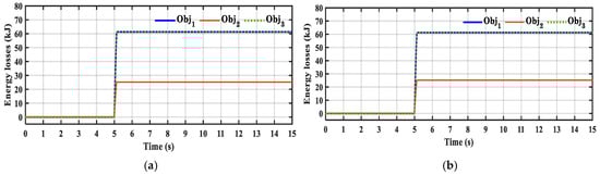
Figure 7. The variation in crowbar energy losses at the 0.8 grid voltage dip for three objective functions: (a) SFO and (b) PSO.

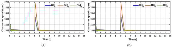
Figure 8. The variation in DFIG speed at the 0.8 grid voltage dip for three objective functions: (a) SFO and (b) PSO.

The optimum values of the crowbar resistance were obtained by two optimization methods: SFO and PSO at 0.8 and 0.6 grid voltage dips. The two methods of optimization were operated for five trials, and the best solution with the lowest value of the objective function was taken. For the two optimization algorithms, the size of the population and the number of iterations are 20 and 20, respectively. The curves of convergence for two optimization methods at the 0.8 grid voltage dip for three objective functions are shown in Figure 9. Figure 10 depicts the convergence curves at the 0.6 grid voltage dip.

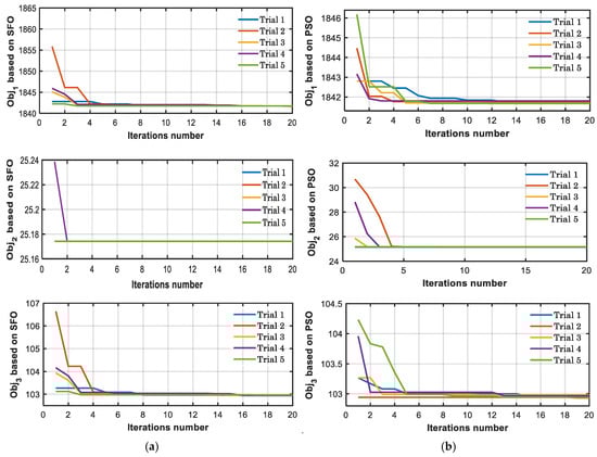
Figure 9. The convergence curve with iterations at the 0.8 grid voltage dip for the three objective functions: (a) SFO and (b) PSO.

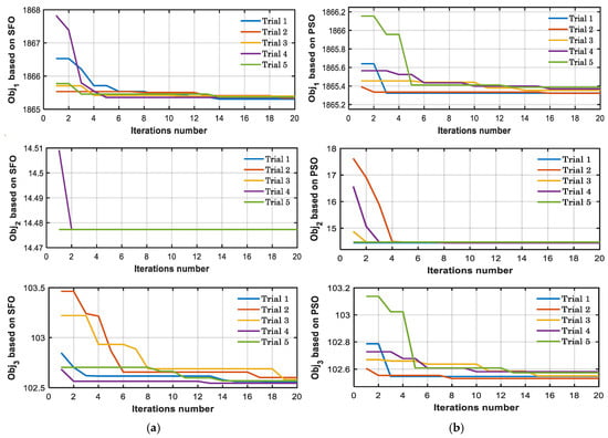
Figure 10. The convergence curve with iterations at the 0.6 grid voltage dip for the three objective functions: (a) SFO and (b) PSO.

Table 3 and Table 4 depict the comparison between the SFO and PSO methods at 0.8 and 0.6 grid voltage dips for three optimization objective functions. The comparison between the two optimization methods is in terms of the elapsed time, the values of the objective function, the maximum DFIG speed, the crowbar energy losses, and the optimum crowbar resistances.

Table 3. The comparison between two optimization techniques at a 0.8 voltage dip.

$\mathit{O}\mathit{b}\mathit{j}$	PSO					SFO
	Elapsed Time (sec)	RCrowbar $(\mathbf{\Omega }$)	Obj	ECrowbar $(\mathbf{k}\mathbf{J}$)	NMax_DFIG (rpm)	Elapsed Time (sec)	RCrowbar $(\mathbf{\Omega }$)	Obj	ECrowbar $(\mathbf{k}\mathbf{J}$)	NMax_DFIG (rpm)
Obj1	68,895.9	0.15756	1841.67	61.248	1841.67	69,619.4	0.15797	1841.68	61.2631	1841.68
Obj2	70,227.5	0.57990	25.14	25.145	1887.70	74,866.6	0.58000	25.17	25.174	1887.70
Obj3	65,981.1	0.15767	102.93	61.217	1841.70	68,113.6	0.15779	102.94	61.217	1841.70

Table 4. The comparison between two optimization techniques at a 0.6 voltage dip.

$\mathit{O}\mathit{b}\mathit{j}$	PSO					SFO
	Elapsed Time (sec)	RCrowbar $(\mathbf{\Omega }$)	Obj	ECrowbar $(\mathbf{k}\mathbf{J}$)	NMax_DFIG (rpm)	Elapsed Time (sec)	RCrowbar $(\mathbf{\Omega }$)	Obj	ECrowbar $(\mathbf{k}\mathbf{J}$)	NMax_DFIG (rpm)
Obj1	78,299.0	0.12127	1865.32	37.22	1865.32	85,616.5	0.12109	1865.31	37.226	1865.31
Obj2	72,308.5	0.57990	14.45	14.449	1898.90	84,171.1	0.58000	14.48	14.477	1898.90
Obj3	69,064.3	0.12094	102.53	37.198	1865.30	74,596.7	0.12098	102.55	37.196	1865.30

Two scenarios were studied to show the effectiveness of the obtained optimal crowbar resistance on the LVRT capability. The first scenario studied the system at a 0.8 grid voltage dip without implementing the crowbar circuit protection. While the second scenario studied the system at a 0.8 grid voltage dip and implementing the crowbar circuit protection. The optimal crowbar resistance, which was obtained from SFO for the third objective function (${Obj}_3$) at the 0.8 grid voltage dip was used in the simulation. Figure 11, Figure 12, Figure 13 and Figure 14 present the simulation results for these two scenarios. Figure 11 shows the grid voltages at the time when the period of the grid voltage dip is 125 msec. Figure 12 demonstrates the variation in DFIG speed and DC-bus voltage, with the time noted for the two scenarios. Figure 13 shows the rotor currents for the two scenarios. Figure 14 shows the stator currents for the two scenarios.

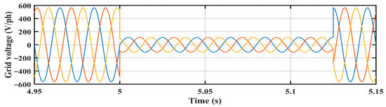
Figure 11. The variation in grid voltages for the two scenarios.

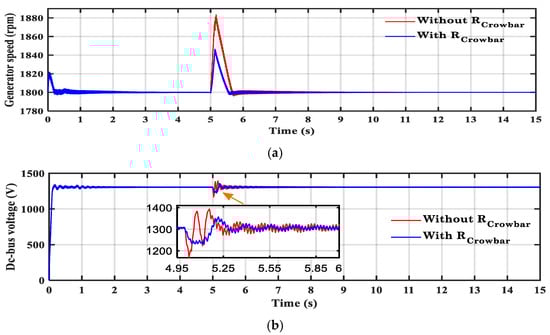
Figure 12. The variation in (a) DFIG speed and (b) DC-bus voltage for the two scenarios.

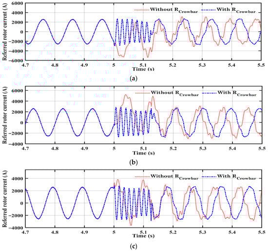
Figure 13. The rotor currents for the two scenarios: (a) phase a, (b) phase b, and (c) phase c.

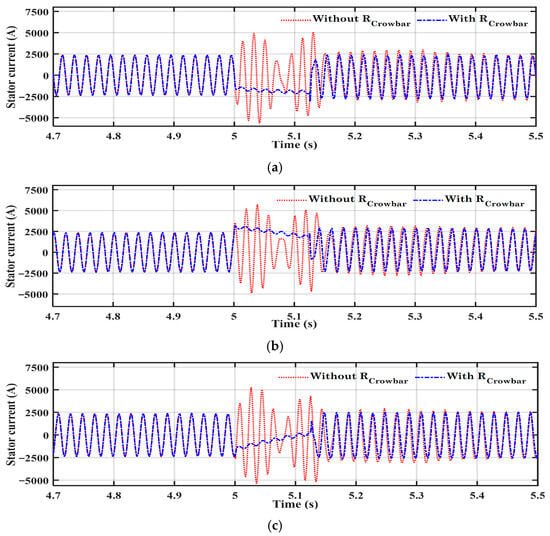
Figure 14. The stator currents for the two scenarios: (a) phase a, (b) phase b, and (c) phase c.

4. Discussion

From the results, it can be concluded that PSO takes slightly less execution time as compared to SFO for most cases. Two optimization methods give roughly similar objective function values. The value of the grid voltage dip does not affect the optimal crowbar resistance. The obtained optimal values of crowbar resistance can achieve the goal for the three objective optimization functions, where the DFIG speed for the first objective function is lower than the DFIG speed for the other two objective functions. The crowbar energy losses for the second objective function are lower than the DFIG speed for the other two objective functions.

By optimizing crowbar resistance, the DC-link voltage rise, and rotor speed overshoot were significantly reduced by 42.5% and 45.8%, respectively, confirming the strategy’s ability to improve system stability during grid faults (at a 13 m/s wind speed and at 0.8, 0.6 grid voltage dips). The results also demonstrated that optimizing the crowbar solely for energy losses reduced energy dissipation by 59% but allowed the generator speed during the fault to reach 1894 rpm. In contrast, optimization focused exclusively on limiting the generator speed effectively, restricting the peak rotor speed to 1846 rpm. From the simulation results for the two scenarios, it is concluded that the system with crowbar protection can ride through the grid voltage dip without increasing the rotor and stator currents exceeding their rated values, and DFIG speed and DC-bus voltage do not increase over their limits.

5. Conclusions

This paper presented the optimal crowbar resistance values for achieving different goals to enhance LVRT capability. Three optimization objectives were taken for minimizing the crowbar energy losses and ensuring stable DFIG operation at different values of grid voltage dips. The comparison between two scenarios, the system with and without implementing the crowbar circuit protection, was introduced to show the effectiveness of the obtained optimal crowbar resistance on the LVRT capability. The results indicated that the optimal crowbar resistance is largely independent of the magnitude of the grid voltage dip. The system with crowbar protection can ride through the grid voltage dip without increasing the rotor and stator currents exceeding their rated values, and DFIG speed and DC-bus voltage do not increase over their limits. This paper outlines several directions for future research, including the following points.

i

Obtaining the optimal crowbar resistance at a broader range of wind speeds and grid voltage dips.

ii

Studying the system under other fault types.

iii

The integration of optimized crowbar resistance with other advanced control strategies, such as adaptive predictive control, may further enhance LVRT performance.

References

- Desalegn, B.; Gebeyehu, D.; Tamrat, B. Wind energy conversion technologies and engineering approaches to enhancing wind power generation: A review. Heliyon 2022, 8, e11263. [Google Scholar] [CrossRef]
- Abdelateef Mostafa, M.; El-Hay, E.A.; Elkholy, M.M. Recent Trends in Wind Energy Conversion System with Grid Integration Based on Soft Computing Methods: Comprehensive Review, Comparisons and Insights. Arch. Comput. Methods Eng. 2023, 30, 1439–1478. [Google Scholar] [CrossRef]
- Mebkhouta, T.; Golea, A.; Boumaraf, R.; Benchouia, T.M.; Karboua, D.; Bajaj, M.; Chebaani, M.; Blazek, V. Sensorless finite set predictive current control with MRAS estimation for optimized performance of standalone DFIG in wind energy systems. Results Eng. 2024, 24, 103622. [Google Scholar] [CrossRef]
- Mostafa, M.A.; El-Hay, E.A.; ELkholy, M.M. Optimal maximum power point tracking of wind turbine doubly fed induction generator based on driving training algorithm. Wind Eng. 2023, 47, 671–687. [Google Scholar] [CrossRef]
- Hamid, B.; Hussain, I.; Iqbal, S.J.; Singh, B.; Das, S.; Kumar, N. Optimal MPPT and BES Control for Grid-Tied DFIG-Based Wind Energy Conversion System. IEEE Trans. Ind. Appl. 2022, 58, 7966–7977. [Google Scholar] [CrossRef]
- Jabal Laafou, A.; Ait Madi, A.; Addaim, A.; Intidam, A. Dynamic Modeling and Improved Control of a Grid-Connected DFIG Used in Wind Energy Conversion Systems. Math. Probl. Eng. 2020, 2020, 1651648. [Google Scholar] [CrossRef]
- Alaboudy, A.H.K.; Mahmoud, H.A.; Elbaset, A.A.; Abdelsattar, M. Technical Assessment of the Key LVRT Techniques for Grid-Connected DFIG Wind Turbines. Arab. J. Sci. Eng. 2023, 48, 15223–15239. [Google Scholar] [CrossRef]
- Mostafa, M.A.; El-Hay, E.A.; Elkholy, M.M. An overview and case study of recent low voltage ride through methods for wind energy conversion system. Renew. Sustain. Energy Rev. 2023, 183, 113521. [Google Scholar] [CrossRef]
- Yadav, M.; Pal, N.; Saini, D.K. Low voltage ride through capability for resilient electrical distribution system integrated with renewable energy resources. Energy Rep. 2023, 9, 833–858. [Google Scholar] [CrossRef]
- Döşoğlu, M.K. Enhancement of LVRT Capability in DFIG-Based Wind Turbines with STATCOM and Supercapacitor. Sustainability 2023, 15, 2529. [Google Scholar] [CrossRef]
- Khosravi, N.; Dowlatabadi, M.; Oubelaid, A.; Belkhier, Y. Optimizing reliability and safety of wind turbine systems through a hybrid control technique for low-voltage ride-through capability. Comput. Electr. Eng. 2025, 123, 110205. [Google Scholar] [CrossRef]
- de Oliveira, I.R.; Tofoli, F.L.; Mendes, V.F. Influence of low-voltage ride-through control techniques on the thermal behavior of power converters applied to wind energy conversion systems based on the doubly-fed induction generator. Electr. Power Syst. Res. 2025, 239, 111272. [Google Scholar] [CrossRef]
- Justo, J.J.; Mwasilu, F.A.; Bansal, R.C. Chapter Twelve—Fault ride through techniques based on hardware circuits for DFIG based wind turbines. In Modeling and Control Dynamics in Microgrid Systems with Renewable Energy Resources; Bansal, R.C., Justo, J.J., Mwasilu, F.A., Eds.; Academic Press: Cambridge, MA, USA, 2024; pp. 313–344. [Google Scholar]
- Kashiv, A.; Verma, H.K. Techniques used for the LVRT ability enhancement for DFIG connected system. In Proceedings of the 2020 First International Conference on Power, Control and Computing Technologies (ICPC2T), Raipur, India, 3–5 January 2020; pp. 68–72. [Google Scholar]
- Reddy, K.; Saha, A.K. A Heuristic Approach to Optimal Crowbar Setting and Low Voltage Ride through of a Doubly Fed Induction Generator. Energies 2022, 15, 9307. [Google Scholar] [CrossRef]
- Kalantarian, S.R.; Heydari, H. An analytical method for selecting optimized crowbar for DFIG with AHP algorithm. In Proceedings of the 2011 2nd Power Electronics, Drive Systems and Technologies Conference, Raipur, India, 16–17 February 2011; pp. 1–4. [Google Scholar]
- Liu, B.; Xu, C.; Gui, J.; Lin, C.; Shao, M. Research on the value of crowbar resistance to low voltage ride through of DFIG. In Proceedings of the 2015 International Conference on Computer and Computational Sciences (ICCCS), Greater Noida, India, 27–29 January 2015; pp. 44–48. [Google Scholar]
- Hu, S.; Zou, X.; Kang, Y. A novel optimal design of DFIG crowbar resistor during grid faults. In Proceedings of the 2014 International Power Electronics Conference (IPEC-Hiroshima 2014—ECCE ASIA), Hiroshima, Japan, 18–21 May 2014; pp. 555–559. [Google Scholar]
- Morsali, P.; Morsali, P.; Ghadikola, E.G. Analysis and Simulation of Optimal Crowbar Value Selection on Low Voltage Ride-Through Behavior of a DFIG-Based Wind Turbine. Proceedings 2020, 58, 18. [Google Scholar]
- Zhu, D.; Wang, Z.; Ma, Y.; Hu, J.; Zou, X.; Kang, Y. Hybrid LVRT Control of Doubly-Fed Variable Speed Pumped Storage to Shorten Crowbar Operational Duration. IEEE Trans. Power Electron. 2024, 39, 14192–14203. [Google Scholar] [CrossRef]
- Mahmoud, M.M.; Benlaloui, I.; Benbouya, B.; Ibrahim, N.F. Investigations on Grid-Connected DFIWGs Development and Performance Analysis with the Support of Crowbar and STATCOM. Control Syst. Optim. Lett. 2024, 2, 191–197. [Google Scholar] [CrossRef]
- Ali, M.A.S. Improved Transient Performance of a DFIG-Based Wind-Power System Using the Combined Control of Active Crowbars. Electricity 2023, 4, 320–335. [Google Scholar] [CrossRef]
- Gebru, F.M.; Khan, B.; Alhelou, H.H. Analyzing low voltage ride through capability of doubly fed induction generator based wind turbine. Comput. Electr. Eng. 2020, 86, 106727. [Google Scholar] [CrossRef]
- Paliwal, P. A State-of-the-Art Review on LVRT Enhancement Techniques for DFIG-Based Wind Turbines. In Advances in Energy Technology, Proceedings of the 1st International Conference on Energy, Materials Sciences, and Mechanical Engineering (EMSME 2020), Delhi, India, 31 October–1 November 2020; Springer: Singapore, 2022; pp. 131–141. [Google Scholar]
- Khajeh, A.; Ghazi, R.; Abardeh, M.H.; Sadegh, M.O. An efficient crowbar to improve the low voltage ride-through capability of wind turbines based on DFIG excited by an indirect matrix converter. Int. J. Power Electron. 2020, 11, 236–255. [Google Scholar] [CrossRef]
- Ahyaten, S.; Bahaoui, J.E. Modeling of Wind Turbines Based on DFIG Generator. Proceedings 2020, 63, 16. [Google Scholar] [CrossRef]
- Mehroliya, S.; Arya, A.; Mitra, U.; Paliwal, P.; Mundra, P. Comparative Analysis of Conventional Technologies and Emerging Trends in Wind Turbine Generator. In Proceedings of the 2021 IEEE 2nd International Conference on Electrical Power and Energy Systems (ICEPES), Bhopal, India, 10–11 December 2021; pp. 1–6. [Google Scholar]
- Mostafa, M.A.; El-Hay, E.A.; Elkholy, M.M. Torque ripple minimization and maximum power point tracking of wind turbine doubly fed induction generator based on bonobo optimization algorithm. Neural Comput. Appl. 2025, 37, 19371–19392. [Google Scholar] [CrossRef]
- Tian, J.; Su, C.; Chen, Z. Reactive power capability of the wind turbine with Doubly Fed Induction Generator. In Proceedings of the IECON 2013—39th Annual Conference of the IEEE Industrial Electronics Society, Vienna, Austria, 10–13 November 2013; pp. 5312–5317. [Google Scholar]
- Al-Quraan, A.; Al-Masri, H.; Al-Mahmodi, M.; Radaideh, A. Power curve modelling of wind turbines—A comparison study. IET Renew. Power Gener. 2022, 16, 362–374. [Google Scholar] [CrossRef]
- Wang, J.; Bo, D.; Miao, Q.; Li, Z.; Wu, X.; Lv, D. Maximum power point tracking control for a doubly fed induction generator wind energy conversion system based on multivariable adaptive super-twisting approach. Int. J. Electr. Power Energy Syst. 2021, 124, 106347. [Google Scholar] [CrossRef]
- Chen, P.; Han, D.; Li, K.C. Robust Adaptive Control of Maximum Power Point Tracking for Wind Power System. IEEE Access 2020, 8, 214538–214550. [Google Scholar] [CrossRef]
- Youssef, A.-R.; Mousa, H.H.H.; Mohamed, E.E.M. Development of self-adaptive P&O MPPT algorithm for wind generation systems with concentrated search area. Renew. Energy 2020, 154, 875–893. [Google Scholar] [CrossRef]
- González-Hernández, J.G.; Salas-Cabrera, R.; Vázquez-Bautista, R.; Ong-de-la-Cruz, L.M.; Rodríguez-Guillén, J. A novel MPPT PI discrete reverse-acting controller for a wind energy conversion system. Renew. Energy 2021, 178, 904–915. [Google Scholar] [CrossRef]
- Liu, M.; Pan, W.; Zhang, Y.; Zhao, K.; Zhang, S.; Liu, T. A Dynamic Equivalent Model for DFIG-Based Wind Farms. IEEE Access 2019, 7, 74931–74940. [Google Scholar] [CrossRef]
- Soomro, M.A.; Memon, Z.A.; Kumar, M.; Baloch, M.H. Wind energy integration: Dynamic modeling and control of DFIG based on super twisting fractional order terminal sliding mode controller. Energy Rep. 2021, 7, 6031–6043. [Google Scholar] [CrossRef]
- El Amine, B.B.M.; Ahmed, A.; Houari, M.B.; Mouloud, D. Modeling, Simulation and Control of a Doubly-Fed Induction Generator for Wind Energy, Conversion Systems. Int. J. Power Electron. Drive Syst. (IJPEDS) 2020, 11, 1197–1210. [Google Scholar] [CrossRef]
- Bossoufi, B.; Karim, M.; Taoussi, M.; Aroussi, H.A.; Bouderbala, M.; Deblecker, O.; Motahhir, S.; Nayyar, A.; Alzain, M.A. Rooted Tree Optimization for the Backstepping Power Control of a Doubly Fed Induction Generator Wind Turbine: dSPACE Implementation. IEEE Access 2021, 9, 26512–26522. [Google Scholar] [CrossRef]
- Dal, M.; Kennel, R.M. A Dynamic Modeling Approach: Simplifying DFIG Theory, Simulation, and Analysis. Energies 2025, 18, 282. [Google Scholar] [CrossRef]
- Elkholy, M.M.; Mostafa, M.A.; El-Hay, E.A. Enhancing steady-state and dynamic performance of wind turbine doubly fed induction generator using AI optimization approaches with adaptive PI controllers. Results Eng. 2025, 26, 104631. [Google Scholar] [CrossRef]
- Zhong, C.; Li, G.; Meng, Z.; Li, H.; Yildiz, A.R.; Mirjalili, S. Starfish optimization algorithm (SFOA): A bio-inspired metaheuristic algorithm for global optimization compared with 100 optimizers. Neural Comput. Appl. 2025, 37, 3641–3683. [Google Scholar] [CrossRef]
- Izci, D.; Ekinci, S.; Jabari, M.; Bajaj, M.; Blazek, V.; Prokop, L.; Yildiz, A.R.; Mirjalili, S. A new intelligent control strategy for CSTH temperature regulation based on the starfish optimization algorithm. Sci. Rep. 2025, 15, 12327. [Google Scholar] [CrossRef]
- Aktaş, M.; Kiliç, F. Discrete Starfish Optimization Algorithm for Symmetric Travelling Salesman Problem. IEEE Access 2025, 13, 102675–102687. [Google Scholar] [CrossRef]
Disclaimer/Publisher’s Note: The statements, opinions and data contained in all publications are solely those of the individual author(s) and contributor(s) and not of MDPI and/or the editor(s). MDPI and/or the editor(s) disclaim responsibility for any injury to people or property resulting from any ideas, methods, instructions or products referred to in the content. |
© 2025 by the authors. Published by MDPI on behalf of the International Institute of Knowledge Innovation and Invention. Licensee MDPI, Basel, Switzerland. This article is an open access article distributed under the terms and conditions of the Creative Commons Attribution (CC BY) license (https://creativecommons.org/licenses/by/4.0/).