Abstract
Warehouses are used to store raw materials, finished goods, defective products, tools, machinery, and other company assets until needed. In addition, the warehouse is a staging area for the storage and packaging of products delivered to the customer for consumer industries. Ideally, storage time, storage space, and delivery lead times are minimized by improving warehouse management. This study implements an integration of linear programming (LP) and decision-making models. The LP model provides decision-makers with the optimum quantity of products that can be stored in the warehouse based on different case scenarios considered in this study. Furthermore, the criteria affecting the space utilization of warehouses at total capacity are identified. An integrated approach of rough analytical hierarchical process (AHP) and rough technique for order preference by similarity to ideal solution (TOPSIS) is utilized to determine the best pallet placement on the respective rack. Additionally, this technique identifies the storage racks that require improvements in warehouse space utilization for the products. This methodological approach will help many industries and logistics teams make optimal decisions and improve productivity.
1. Introduction
Currently, organizations in the global market optimize their warehouses to improve production capacity and distribution, reduce lead and delivery times, and maintain sufficient inventory to meet seasonal demand [1,2]. In this highly competitive global market, various organizations and industries must become extremely efficient and must implement continuous improvement methods to maintain their performance indices [3,4].
Successful businesses are employing technological advances in monitoring, storing, and shipping goods worldwide to eliminate waste, reduce cost, and improve customer service [5,6]. In addition, companies incorporate effective supply chain logistics and lean manufacturing techniques integrated with Industry 4.0 principles, which improve product delivery and increase customer satisfaction, leading to viability and improved profit margins [7].
Various chain management techniques have been implemented to monitor the warehouse and maximize inventory to leverage the storage of the products [8]. Warehouse management plays a crucial role in the successful operation of businesses. The global market relies on innovative techniques to improve the workflows in the warehouses of various industries [4]. For example, the implementation of radio frequency identification (RFID) tags on the products, through which serial numbers or bar codes are scanned in the system, allows the product location to be identified along with an estimated delivery time [9]. Furthermore, various inventory management software applications are available for maintaining proper inventory. This software provides the required information when the replenishment of the stock is needed to restore the inventory in the organization’s warehouse [5]. To establish a workflow, optimize the process, and increase the workforce efficiency within the industry or production plant, different decision-making approaches are available: optimization-based, i.e., linear programming, genetic algorithm; simulation-based, i.e., discrete event; and multi-criteria decision-making analysis (MCDA), i.e., weighted sum approach (WSA), analytic hierarchy process (AHP), and technique for order preference by similarity to ideal solution (TOPSIS) [10,11,12,13,14].
This study focuses on improving supplier warehouse utilization and maximizing in-plant warehouse utilization by optimizing the storage space for current product demands. Key considerations include storage space utilization, rack layout, the number of units per shelf, warehouse dimensions, and layout. In addition, this study aims to provide maximum quantities for product storage and decision-making guidance to determine the best placement of the product for optimal product storage, retrieval, and shipping to the customer.
Therefore, the objectives of this study are summarized as the following:
- Implement a linear programming (LP) model to determine the maximum quantity of boxes that can be stored on the respective rack of the warehouse;
- Identify criteria that can maximize the utilization of the warehouse;
- Develop a decision-making model based on the criteria concerning the storage rack to optimize the ranking of box placement.
To achieve these objectives, this study integrates both the optimization- and MCDA-based methods. The dimensional data regarding the warehouse and product box are analyzed to formulate the LP model. The best possible solution from this model maximizes the quantities of the boxes stacked on the shelves within the facility. Furthermore, the type and number of products that can be placed on the shelves are defined. Then, the most suitable and effective placement for the product can be obtained through the decision-making tool, which is developed by integrating the rough AHP method with the rough TOPSIS method [15]. Rough set theory plays a vital role in handling the uncertainties and provides appropriate decisions by removing the vagueness of the experts’ opinions.
2. Literature Review
Various researchers have conducted notable studies for warehouse and inventory management. For example, Altarazi and Ammouri [10] developed a simulation-based decision-making tool to evaluate the warehouse model which enables the decision-makers and logistics team to select sufficient labor requirements and use the warehouse space effectively. The data considered in the model creation included the warehouse dimensions, rack location, and rack dimensions. Their model was rendered in Arena software using volume-based storage. In another study, Janssens and Ramaekers [16] developed an LP model for inventory management and cost analysis. Furthermore, Lerher et al. [17] discussed the multiple objective optimizations of the warehouse, using the genetic algorithm to find the Pareto optimal solution. The authors developed the mathematical model based on objective functions such as minimizing travelling time, minimizing cost, and maximizing the quality of the warehouse.
To optimize the space utilization of a storage rack in the garment industry in India, Shetty et al. [11] presented an LP model that uses box dimensions, product quantity, and production values. The authors optimized the number of racks in use in warehouse storage, and, using the ABC analysis, the optimized solution allocates the materials in sequential order.
He et al. [18] developed a novel stochastic MCDA model for emergency warehouse locations in the case of a natural disaster in China. This study accounted for the traffic conditions, stock holding capacity, surrounding environment for reserving relief supply, distance to the disaster-prone area, and cost criteria for the analysis. The authors used the ELimination and ChoiceExpressingREality (ELECTRE)-II methods for the selection of the emergency warehouse location.
Kusrini et al. [12] developed a decision-making framework for warehouse performance measurement to improve the efficiency of logistics systems. The authors suggested key performance indicators (KPIs), and the most significant KPI was determined using AHP. Based on the consistency ratio and KPI weights, the warehouse performance was evaluated and analyzed. The SNORM De Boer normalization process method was employed to obtain the final KPI scores and improve the warehouse efficiency.
Similarly, Stopka and Ľupták [9] conducted the optimization of warehouse management within an assembly and distribution company. The authors considered the cost of realization, cost of labelling per piece, handling in case of damage, and other information contained in the analysis and used the traditional weighted sum approach (WSA) to determine the weights of the criteria. Then, they used the TOPSIS method to rank the two alternatives (barcodes and RFID).
Al Amin et al. [13] developed a decision-making model for the warehouse location selection depending on unit price, stockholding capacity, average distance to the factory, flexibility, and layout. The weights of the criteria were determined using AHP, while the warehouses were ranked using the TOPSIS method. In another study, Bao et al. [8] discussed storage assignment strategies and route planning of automated guided vehicle systems in warehouse operation optimization. The authors implemented a simulation-based method to determine the storage location and optimal route for vehicles to travel in a traditional rectangular two-block layout warehouse.
Kordos et al. [14] utilized genetic algorithms for the optimization of discrete product placement and order-picking routes in a warehouse. In this model, the cost of the given product placement is expressed as the sum of the lengths of the optimized order-picking routes. Finally, Islam et al. [4] proposed a particle swarm optimization-based grey model to predict the performance of a readymade garment warehouse. The authors considered KPIs related to cost, time, productivity, and quality, and predicted warehouse performance using grey-based models. A few studies use the integrated approach of linear-equation and decision-making analysis, but this study provides the analysis for the warehouse space utilization and most suitable placement of the product.
3. Methodology
In this study, various elements were considered to maximize the storage space utilization in a warehouse. First, qualitative and quantitative data needed to optimize the warehouse were collected based on the literature review and feedback from experts. The data were collected using an online survey and email, following the methodology framework implemented in this study. Next, the LP model was formulated to determine the maximum number of boxes that could be stored in the supplier warehouse. Then, the results of the survey provided the necessary information to develop a decision-making tool. This tool uses the linguistic scale values and the scale of importance values based on responses from the decision-makers. In addition, rough AHP and rough TOPSIS methods were used to obtain the ranking for the best placement of the product based on the criteria. Figure 1 shows the proposed framework. The methods are discussed in detail in the following subsections.
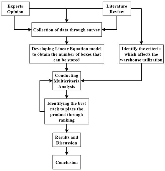
Figure 1.
Proposed framework.
3.1. Linear Programming
LP is an optimization technique used to determine the optimal solution for a defined objective function, constraints, and decision variables [11,19]. The LP solution is determined by maximizing or minimizing the objective function. LP is a straightforward optimization technique with a wide range of applications. The basic terminology used in LP is as follows [19]:
- Objective function. The objective function determines the end outcome of the linear equation, which is maximization or minimization. For example, profit is a maximization function based on the given information.
- Constraint. The constraints are predetermined on the objective function to control the linear equation such that it does not exceed the set limit, such as the quantity of the product placed on the shelves.
- Decision variable. The decision variables, or the end output, need to be identified. This set of variables is denoted with x or y based on the linear equation formulation.
- Non-negativity. Non-negativity is a restriction for a decision variable to be greater than or equal to zero.
The following steps are followed to formulate the LP model [19].
- Step A1: Highlight the essential key variables.
- Step A2: Identify the decision variables that need to be optimized.
- Step A3: Formulate the objective function.
- Step A4: Identify the constraints from the given data.
- Step A5: Solve the linear equation model and analyze the results.
3.2. Criteria Selection for Warehouse
The first step is to identify the criteria, or key variables, that can have a positive or a negative effect depending on the situation. The selection of criteria is vital for the MCDA to determine the best placement of the boxes. Since the main goal is to optimize the warehouse by maximizing storage space to minimize transportation or pallet movement between departments, additional factors should be considered. Table 1 describes the criteria selected based on the literature [2,7,9,12,20] ( and feedback from the experts. In this study, access to all areas (C1), order characteristic (C2), the frequency of the product (C3), and material handling (C6) are the cost criteria, and storage area (C4) and the placement of the product (C5) are the benefit criteria.

Table 1.
Criteria that affect the warehouse space utilization.
3.3. Analytical Hierarchical Process
After obtaining the criteria, the AHP analysis is performed. AHP is an MCDM technique used to analyze and organize complex decisions in complex environments where different constraints, criteria, and variable factors are considered for prioritization. This approach provides a structural understanding of a given problem. The problem is divided into a hierarchy of criteria to be analyzed quickly and compared individually based on the weights provided by the decision-makers [21]. First, the pairwise comparison matrix is constructed according to the scale of relative importance provided in Appendix A (Table A1).
The following steps are followed for the AHP analysis of the criteria obtained from the literature study that can affect the supplier warehouse [22].
Step B1: Develop a decision matrix based on the scale of importance. The decision-maker provides the values used in the pairwise matrix based on the scale of relative importance. A sample pairwise matrix is shown in Table A2.
Step B2: Obtain the weights of the criteria by dividing the individual geometric mean by the total geometric mean.
Step B3: Determine λmax by performing a matrix multiplication of the weights with respect to the sum of the scale of importance. Then, the consistency index (CI) is determined by using the following formula:
where n is the number of criteria. Finally, the consistency ratio (CR) is calculated by dividing the CI by the random index (RI), the values of which are presented in Table A3.
3.4. Rough Analytic Hierarchy Process (AHP)
The rough set theory was developed to handle the subjective judgment of the decision-makers when determining the boundary intervals, which are later integrated with the arithmetic operation to generally analyze complex and vague information. Thus, in this case, the consistency of preferences is measured while the judgment made by the decision-makers is managed. In addition, the rough set theory is utilized to solve and eliminate uncertainties, which include the vagueness of the judgment or the opinion of an expert who may not have experience in the related field. Furthermore, experts are asked to provide the scale of importance to evaluate the criteria for a particular problem. Therefore, the rough set theory evaluates the given criteria within a small set of data, lowering the uncertainty to provide the best decision. The following steps are followed to develop the rough AHP tool [21,22,23]:
Step C1: Develop a multiple decision-making pairwise matrix formed by the expert’s team working in the warehouse, the same matrix considered during the AHP process.
Step C2: After determining the crisp value, obtain the rough numbers by following a series of equations.
Consider U as the universe consisting of all the objects, and X is considered a random object from universe U. The following assumption in Equation (2) is a specific set built with the decision-makers’ preferences.
with the given condition:
Then, for , the lower approximation and upper approximation are determined.
Lower approximation:
Upper approximation:
Step C3: Define the random object X with the rough number R.N. with the lower limit and upper limit :
where and represent the sums of objects in the lower and upper object approximation of , respectively.
Step C4: Create a rough comparison matrix consisting of rough numbers following Equation (7):
where is the lower limit of the rough number R.N. () and is the upper limit of the rough number R.N. (). Then, the average rough number limits are taken as
where and are the average lower and upper limits of rough number R.N. ().
The rough comparison matrix is constructed in the same following step as
Step C5: Obtain the weight of each criterion by applying the power root for the weights obtained using Equation (11):
Finally, the weights are normalized:
3.5. Rough Technique for Order Preference by Similarity to Ideal Solution (TOPSIS)
The weights of the criteria obtained from the previous rough AHP process are used to obtain the ranking by following the procedure for the rough TOPSIS method. The rough TOPSIS, a hybrid method for analyzing multiple-decision-maker problems, combines the rough set theory and the TOPSIS method [15,24,25]:
Step D1: Develop a matrix by compiling the data of the decision-makers, such that the performance values of each alternative or rack are compared using the scale provided in Table A4 with respect to the criteria.
Step D2: After obtaining the crisp value, calculate the rough numbers by following Equations (2)–(9) to construct the rough matrix for the TOPSIS analysis as follows:
Step D3: Evaluate the standardized decision matrix with respect to the rough number using the Equations (14) and (15):
where and are the lower and upper limits of the standardized rough matrix, respectively.
Step D4: Determine the weighted standardized rough matrix by multiplying the standardized rough number from the previous step with the weights obtained from the rough AHP method:
Step D5: Obtain the positive and negative ideal solutions using Equations (18) and (19):
where and denote the positive and negative ideal solution, respectively, and B and C represent the beneficial and cost criteria, respectively.
Step D6: Obtain the ranking using Equations (20) and (21):
where and are the separation distance of each alternative from the positive and negative ideal solution, respectively. The closeness coefficient is evaluated for each value by the following equation:
Finally, the ranking of the rack is obtained based on the descending order of the closeness coefficient.
4. Framework Implementation
The proposed framework was implemented to optimize Decathlon’s supplier warehouse. Decathlon, a prominent distributor of various types of sporting goods, is a French retail organization with nearly 1709 outlets in more than a thousand cities and 60 countries [26]. The company is rapidly expanding its business and growing sales in the global market. This section describes the step-by-step implementation of the developed framework.
4.1. Implementation of Linear Programming
To identify the best placement in the warehouse, optimizing the transportation or minimizing the pallet movement, data were collected from the logistics department of Decathlon. Table 2 highlights the dimensions of the warehouse, rack, shelf, box, and pallet. Table 3 presents the box quantities based on the percentage and additional information based on the number of products that can be stored in the box. Table 4 shows the weekly product demand from July 2020 to October 2020 based on the information provided by the supplier.
Table 2.
Warehouse, rack, shelves, box, and pallet dimensions.
Table 3.
Box quantities and information based on the percentage and number of products.
Table 4.
Weekly product demand from July to October.
The steps from Section 3.1 were followed to formulate the LP model:
Step A1: Highlight the essential key variables that are needed for the model development.
Step A2: Identify the decision variables that need to be optimized, and include the given data:
The decision variables in this warehouse study are the number of boxes that can be stored on each pallet and placed on the shelves.
- Quantity of Box 1 thatcan be stored on the rack = x1
- Quantity of Box 2that can be stored on the rack = x2
- Quantity of Box 3that can be stored on the rack = x3
Step A3: Formulate the objective function.
The objective of this optimization model is to maximize space utilization by placing the maximum number of boxes on the pallets at their respective rack in the warehouse. Since Decathlon’s supplier uses the exact pallet dimensions provided in Table 2, the same volume of the pallets is used in the following equation for the objective function:
Step A4: Identify the constraints from the given data provided by the industries and incorporate these limits into the objective functions and decision variables.
The main limitations for the warehouse are the total volume of the rack space, which is 2793.648 m3, and the percentage of the boxes that are initially stored on the shelf with the respective box dimensions. Therefore, the objective function is subject to the following:
where:
All variables are non-negative, i.e.,
Therefore, the LP formulation for Case 1—limitation based on the percentage of the boxes—follows:
Subject to:
where:
All variables are non-negative, i.e.,
The LP formulation for Case 2—maximize the warehouse space to 100% and determine the maximum number of boxes that can be stored—follows:
Subject to:
where:
All variables are non-negative, i.e.,
The LP formulation for Case 3—maximize the number of boxes that can be stored based on the monthly product demand—follows. The constraints consider the total number of boxes that can be stored, and other limitations include the number of products stored in the respective boxes based on the information from Table 2 and Table 3.
Subject to:
where:
All variables are non-negative, i.e.,
The LP formulation for Case 4—maximize the number of boxes that can be stored based on the weekly product demand—follows. The constraints consider the total number of boxes that can be stored, and the other limitations include the number of products stored in the respective boxes based on the information from Table 2 and Table 3.
Subject to:
where:
All variables are non-negative, i.e.,
Step A5: Solve the optimization models and analyze the results.
4.2. Implementation of the AHP Model
In this case study, seven decision-makers were considered in the formulation of the pairwise matrix. These decision-makers had years of experience in warehouse management and operation (Table A5). The pairwise comparison matrix for decision-maker 1 (Step B1) and weights of the criteria (Step B2) are shown in Table A2. Similarly, the pairwise comparison matrices of the other six decision-makers were determined, as highlighted in Table A6. The weights of the criteria based on the judgment of seven decision-makers are summarized in Table A7 and Figure 2.
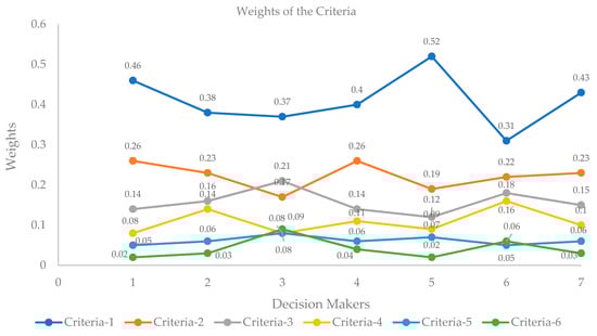
Figure 2.
Weight of the criteria provided by seven decision-makers using AHP method.
4.3. Implementation of Rough AHP Model
To evaluate the criteria and reduce the uncertainties of the decision-makers, the rough AHP method is utilized at this stage. Table A6 summarizes the crisp values of the combined decision matrix for rough AHP (Step C1). The rough number is obtained using the Equations (2)–(9) (Steps C2–C3), as noted in Table 5 in the form of the lower and upper limits (Step C4). Then, the weights and normalized weights of the criteria are calculated (Step C5) using Equations (11) and (12), respectively, and are presented in Table 5.
Table 5.
Rough number of the combined decision matrix.
4.4. Implementation of Rough TOPSIS Model
Firstly, the pairwise decision matrix for the rack with respect to the criteria affecting warehouse performance was developed based on the linguistic values shown in Table A4 (Step D1). Table A7 provides the performance table by decision-maker 1. Similarly, the crisp performance-evaluation values provided by the seven decision-makers were combined, as shown in Table A8. The corresponding rough numbers were obtained (Step D2) using the Equations (2)–(9), as highlighted in Table A9. Table A10 shows the standardized decision matrix of rough numbers using Equations (14) and (15) (Step D3). The weighted standardized decision matrix of rough numbers was calculated (Step D4) using Equations (16) and (17), as shown in Table A11. The positive and negative ideal solutions based on the type of the criteria are presented in Table A12. Next, the separation distance of each alternative from the positive and negative ideal solutions was determined (Step D5) using Equations (20) and (21), respectively (Table A13). Finally, the racks were ranked based on the closeness coefficient, as shown in Table 6.
Table 6.
Separation distances and the ranking of each rack.
5. Result and Discussion
5.1. Results of Linear Programming
For Case 1 (Section 4.1), warehouse utilization is based on the demand box percentage and maximum limits provided by the company. The limitations are the percentage of boxes: x1 = 55 to 60%, or 7200 boxes; x2 = 20 to 30%, or 3600 boxes; and x3 = 10 to 25%, or 1200 boxes. Using the LP Excel Solver, the analysis found that a storage rack volume of 475.188 m3 is used compared to the total volume of the warehouse of 2793.648 m3. The given variable constraint and the maximum box limits are reached. Opportunities for improvement are available since only 17.01% of the warehouse storage is utilized, leading to the consideration of Case 2.
Case 2 (Section 4.1) looks at maximizing the full warehouse space and determining the maximum quantity of each box based on the demand percentage. The main motive is to maximize the utilization of the warehouse rack space, and the values of the variables are increased six-fold: x1 ≤ 43,200; x2 ≤ 21,600; and x3 ≤ 7200. The results for Case 2 showed that 100% of the warehouse storage space is utilized, and the quantities of Box 1, Box 2, and Box 3 that can be stored are 42,002, 21,600, and 7200 units, respectively. These variables increased significantly by 483 to 500% compared to Case 1, and the warehouse utilization is 100%. Furthermore, the optimum quantity of products that can be stored on shelves can be 70,802 boxes. The logistics team can decide on the quantity of product which can be stored on the respective shelves.
For Case 3 (Section 4.1), the limitations are based on the products’ monthly demand (i.e., July–October) and the total number of units stored in their respective boxes. In this case, the percentages of boxes are considered, following the supplier warehouse standards provided by the respective department. Therefore, the percentages of boxes with respect to the number of products are as follows: x1 = 55 to 60%, or 4,032,000 products in Box 1; x2 = 20 to 30%, or 1,152,000 products in Box 2; and x3 = 10 to 25%, or 288,000 products in Box 3. The results for Case 3 show that the optimum quantities of boxes the supplier needs to store in the warehouse are 91,660 of Box 1, 57,600 of Box 2, and 19,200 of Box 3 to meet the customer demand over the four-month period that is considered peak season for the supplier warehouse. Considering the weekly supply, the optimum storage quantities are 5729 of Box 1, 3600 of Box 2, and 1200 of Box 3, totaling 10,529 boxes per week to meet customer demand.
Finally, in Case 4 (Section 4.1), the limitations are based on the weekly product demand and the total number of units that can be stored in their respective boxes. Similar to Case 3, the optimum quantity of products that can be stored in the warehouse based on the weekly product demand is determined. The percentages of boxes with respect to the number of products are as follows: x1 = 55 to 60%, or 288,000 products; x2 = 20 to 30%, or 90,000 products, and x3 = 10 to 25%, or 24,000 products. The results for Case 4 show that the optimum quantities of boxes the supplier needs to store in the warehouse are 5343 of Box 1, 4500 of Box 2, and 1600 of Box 3 to meet customer demand over a week, totaling a minimum of 11,443 boxes.
When comparing the cases for the LP, Case 1 and Case 2 focus on warehouse utilization with respect to the number of boxes required to fill its capacity; Case 3 and Case 4 focus on the customer demand for the product, such that the supplier stores the minimum quantities of boxes in the warehouse according to the required units ordered. Therefore, with these cases, the supplier can change the warehouse based on the organization’s requirement based on linear programming.
5.2. Analysis Results of AHP and Rough AHP
Figure 2 shows that C1 (access to all areas) and C2 (order characteristics) are the most critical criteria based on the importance levels provided by all the decision-makers. On the other hand, the least important criteria according to all decision-makers based on weight were C6 (material handling) and C5 (placement of the product). The average weights of the criteria are also presented in Table A6. The method implemented was the rough set theory using AHP, which could determine a better CI quickly and could analyze the complex problem. These rough sets are generally utilized for conditions with multiple decision-makers. In this case, some inconsistency may occur using only AHP methods, so for better judgment, the rough method was considered. Moreover, with the aforementioned series of steps and computations of weights based on decision-maker judgments, the C2 (order characteristic), C3 (frequency of product), and C4 (storage area) are consistent, C5 (placement of boxes) and C6 (material handling) have the least weighting, and C1 (access to all areas) has the most influence (Figure 3). These criteria affect the space utilization of the warehouse, as shown in Figure 3.
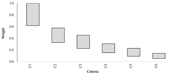
Figure 3.
Weight of the criteria using rough AHP method.
5.3. Results of Rough TOPSIS
Finally, this study applied the rough TOPSIS method to rank the racks based on suitability. Table 6 shows the computed ranking using the following information: the linguistic scale based on input from the decision-makers (Table A9), the crisp numbers generated for all the racks (Table A10), the rough TOPSIS results (Table A10, Table A11, Table A12 and Table A13), and the weights obtained from the rough AHP. Racks 14, 12, 15, and 2 were found to be the most suitable racks in the warehouse for the placement of the high-demand products with respect to the effects of all the criteria in the respective rack. From Table 6, the ranking sequence of the rack with respect to the criteria affecting the storage of the boxes is Rack-14 > Rack-12 > Rack-15 > Rack-2 > Rack-8 > Rack-4 > Rack-5 > Rack-6 > Rack-3 > Rack-7 > Rack-13 > Rack-10 > Rack-11 > Rack-1 > Rack-9.
6. Conclusions
This study was conducted to improve the utilization of a supplier warehouse. The developed framework was implemented to enhance Decathlon’s supplier warehouse, focusing on the optimization of the number of boxes that can be stored and the storage space based on the placement of boxes in the rack based on the ranking using the decision-making tool. Using the boxes’ dimensions, quantities of boxes, number of products in each box, and rack volume, a linear equation was formulated, constrained by the rack volume of 2793.648 m3. The results of Case 2 showed that the warehouse can be utilized up to 100% with an increase in box intake and storage. A total of 70,802 boxes can be stored in the warehouse, which is an increase over the initial number by 483%. Therefore, the optimum quantity of boxes stored on the shelves is between 10,196 and 70,802 boxes.
Case 3 and Case 4 address the customer demand and the optimum inventory to meet the required weekly and monthly targets. For Case 3, to meet the product demands for July to August, the supplier warehouse requires 168,460 boxes, or 42,115 boxes per month. In Case 4, to meet the customer’s weekly demand, the warehouse needs 11,443 boxes. Since the demand continuously fluctuates, depending on the season and customer requirements, these quantities are not constant.
In this study, access to all areas, order characteristics, product frequency, and material handling are the cost criteria, while storage area and placement of the product are the benefit criteria. Based on the results of the rough AHP, the logistics team needs to improve the production and focus on the cost criteria. The results from the decision-making tool indicate that Racks 14, 12, 15, and 2 are the most suitable locations for the products, providing convenience for the receiving and shipping departments. Racks 3, 7, 13, 10, 11, 1, and 9 have the least preference for the high-demand product. The rearrangement of the racks based on the results can introduce additional positive outcomes.
This approach can be implemented to improve the storage facility in an organization or distribution service that owns a warehouse. The tool developed in this study will help the decision-makers and logistics teams of various industries to make better decisions and improve production.
Suggestions for future work include using fuzzy scale models, interpretive structural modelling ISM, and decision-making trial and evaluation laboratory models. These are based on the cause and effect relationship, potentially providing better understanding of the criteria with respect to the rack selection. Additionally, area simulation can be conducted to focus on the product inflow and outflow. Moreover, the workflow of the whole warehouse can be simulated to obtain more useful results in comparison with those obtained in the LP model. Various other decision-making tools can be utilized for similar studies, such as preference ranking organization method for enrichment of evaluations (Promethee), which may provide more refined solutions.
Author Contributions
Conceptualization, S.M., D.S., G.K. and S.S.; methodology, S.M., D.S., G.K. and S.S.; software, S.M.; validation, S.M., D.S., G.K. and S.S.; formal analysis, S.M.; investigation, S.M.; resources, S.M., D.S., G.K. and S.S.; data curation, S.M.; writing—original draft preparation, S.M.; writing—review and editing, D.S. and G.K.; visualization, S.M.; supervision, D.S. and G.K.; project administration, D.S., G.K. and S.S. All authors have read and agreed to the published version of the manuscript.
Funding
Not applicable.
Institutional Review Board Statement
Not applicable.
Informed Consent Statement
Not applicable.
Data Availability Statement
The anonymized data are available from the corresponding author.
Acknowledgments
The authors would like to acknowledge Md Ainul Kabir and Faiza Awad Engdal Nielsen for their support and cooperation to complete this study. The authors would like to thank the experts in providing their feedback for performing this study.
Conflicts of Interest
The authors declare no conflict of interest.
Appendix A
Table A1.
Table for the scale of relative importance for the pairwise comparison matrix.
Table A1.
Table for the scale of relative importance for the pairwise comparison matrix.
| Scale | Relative Importance |
|---|---|
| 1 | Equal Importance |
| 3 | Moderate Importance |
| 5 | Strong Importance |
| 7 | Very Strong Importance |
| 9 | Extreme Importance |
| 2, 4, 6, 8 | Intermediate Values |
| 1/3, 1/5, 1/7, 1/9 | Values for Inverse Comparison |
Table A2.
Sample pairwise comparison matrix for decision-maker 1.
Table A2.
Sample pairwise comparison matrix for decision-maker 1.
| Criteria | C1 | C2 | C3 | C4 | C5 | C6 | Geometric Mean | Weights |
|---|---|---|---|---|---|---|---|---|
| C1 | 1 | 4 | 8 | 5 | 6 | 9 | 4.529 | 0.46 |
| C2 | 1/4 | 1 | 3 | 8 | 6 | 8 | 2.569 | 0.26 |
| C3 | 1/8 | 1/3 | 1 | 7 | 3 | 7 | 1.352 | 0.14 |
| C4 | 1/5 | 1/8 | 1/7 | 1 | 6 | 8 | 0.745 | 0.08 |
| C5 | 1/6 | 1/6 | 1/3 | 1/6 | 1 | 8 | 0.481 | 0.05 |
| C6 | 1/9 | 1/8 | 1/7 | 1/8 | 1/8 | 1 | 0.177 | 0.02 |
| Sum | 1.85 | 5.75 | 12.62 | 21.29 | 22.13 | 41.00 | 9.86 |
Table A3.
Consistency index table.
Table A3.
Consistency index table.
| n | 1 | 2 | 3 | 4 | 5 | 6 | 7 | 8 | 9 | 10 |
|---|---|---|---|---|---|---|---|---|---|---|
| Random Index (RI) | 0.00 | 0.00 | 0.58 | 0.90 | 1.12 | 1.24 | 1.32 | 1.41 | 1.45 | 1.49 |
Table A4.
Table of linguistic values.
Table A4.
Table of linguistic values.
| Scale Values | Scale |
|---|---|
| 1 | Poor Importance |
| 3 | Medium Importance |
| 5 | Fair Importance |
| 7 | Strong Importance |
| 9 | Extreme Importance |
| 2, 4, 6, 8 | Intermediate Values |
Table A5.
Decision-makers and years of experience.
Table A5.
Decision-makers and years of experience.
| Decision-Makers | Years of Experience |
|---|---|
| Decision-Maker 1 | Not Available |
| Decision-Maker 2 | 13 |
| Decision-Maker 3 | 2.5 |
| Decision-Maker 4 | Not Available |
| Decision-Maker 5 | 10 |
| Decision-Maker 6 | 4.5 |
| Decision-Maker 7 | 8 |
Table A6.
Crisp values of combined decision matrix for rough AHP.
Table A6.
Crisp values of combined decision matrix for rough AHP.
| C1 | C2 | C3 | C4 | C5 | C6 | |
|---|---|---|---|---|---|---|
| C1 | 1, 1, 1, 1, 1, 1, 1 | 4, 3, 3, 7, 5, 3, 4 | 8, 1, 3, 4, 7, 5, 5 | 5, 7, 6, 2, 6, 7, 6 | 6, 5, 3, 8, 8, 1/5, 4 | 9, 7, 2, 3, 9, 7, 5 |
| C2 | 1/4, 1/3, 1/3, 1/7, 1/5, 1/3, 1/4 | 1, 1, 1, 1, 1, 1, 1 | 3, 1, 1/2, 5, 7, 5, 3 | 8, 7, 4, 6, 7, 1/3, 4 | 6, 5, 2, 3, 1/2, 7, 4 | 8, 3, 2, 8, 7, 5, 4 |
| C3 | 1/8, 1, 1/3, 1/4, 1/7, 1/5, 1/5 | 1/3, 1,2, 1/5, 1/7, 1/5, 1/3 | 1, 1, 1, 1, 1, 1, 1 | 7, 1/3, 4, 3, 3, 5, 3 | 3, 5, 2, 7, 6, 5, 5 | 7, 3, 2, 2, 7, 6, 5 |
| C4 | 1/5, 1/7, 1/6, 1/2, 1/6, 1/7, 1/6 | 1/8, 1/7, 1/4, 1/6, 1/7, 3, 1/4 | 1/7, 3, 1/4, 1/3, 1/3, 1/5, 1/3 | 1, 1, 1, 1, 1, 1, 1 | 6, 5, 2, 4, 6, 5, 4 | 8, 7, 2, 5, 7, 7, 5 |
| C5 | 1/6, 1/5, 1/3, 1/8, 1/8, 5, 1/4 | 1/6, 1/5, 1/2, 1/3, 2, 1/7, 1/4 | 1/3, 1/5, 1/2, 1/7, 1/6, 1/5, 1/5 | 1/6, 1/5, 1/2, 1/4, 1/6, 1/5, 1/4 | 1, 1, 1, 1, 1, 1, 1 | 8, 7, 1, 7, 9, 1/7, 6 |
| C6 | 1/9, 1/7, 1/2, 1/3, 1/9, 1/7, 1/5 | 1/8, 1/3, 1/2, 1/8, 1/7, 1/5, 1/4 | 1/7, 1/3, 1/2, 1/2, 1/7, 1/6, 1/5 | 1/8, 1/7, 1/2, 1/5, 1/7, 1/7, 1/5 | 1/8, 1/7, 1, 1/7, 1/6, 7, 1/6 | 1, 1, 1, 1, 1, 1, 1 |
Table A7.
Weights of the criteria using AHP method.
Table A7.
Weights of the criteria using AHP method.
| DM1 | DM2 | DM3 | DM4 | DM5 | DM6 | DM7 | Average | |
|---|---|---|---|---|---|---|---|---|
| C1 | 0.46 | 0.38 | 0.37 | 0.40 | 0.52 | 0.31 | 0.43 | 0.41 |
| C2 | 0.26 | 0.23 | 0.17 | 0.26 | 0.19 | 0.22 | 0.23 | 0.22 |
| C3 | 0.14 | 0.16 | 0.21 | 0.14 | 0.12 | 0.18 | 0.15 | 0.16 |
| C4 | 0.08 | 0.14 | 0.08 | 0.11 | 0.09 | 0.16 | 0.10 | 0.11 |
| C5 | 0.05 | 0.06 | 0.08 | 0.06 | 0.07 | 0.05 | 0.06 | 0.06 |
| C6 | 0.02 | 0.03 | 0.09 | 0.04 | 0.02 | 0.06 | 0.03 | 0.04 |
Table A8.
Sample performance table of decision-maker 1.
Table A8.
Sample performance table of decision-maker 1.
| C1 | C2 | C3 | C4 | C5 | C6 | |
|---|---|---|---|---|---|---|
| A1 | 2 | 5 | 7 | 8 | 6 | 3 |
| A2 | 2 | 5 | 7 | 7 | 6 | 3 |
| A3 | 2 | 4 | 5 | 7 | 6 | 5 |
| A4 | 1 | 4 | 6 | 8 | 7 | 8 |
| A5 | 1 | 4 | 6 | 8 | 7 | 8 |
| A6 | 3 | 8 | 7 | 4 | 4 | 9 |
| A7 | 6 | 8 | 2 | 5 | 4 | 5 |
| A8 | 6 | 4 | 4 | 5 | 4 | 6 |
| A9 | 7 | 5 | 5 | 6 | 6 | 9 |
| A10 | 6 | 5 | 5 | 6 | 5 | 8 |
| A11 | 5 | 8 | 5 | 6 | 7 | 8 |
| A12 | 2 | 4 | 2 | 3 | 4 | 7 |
| A13 | 6 | 7 | 7 | 6 | 6 | 8 |
| A14 | 4 | 3 | 4 | 6 | 4 | 8 |
| A15 | 6 | 2 | 4 | 4 | 6 | 9 |
Table A9.
Crisp values of combined decision matrix for rough TOPSIS.
Table A9.
Crisp values of combined decision matrix for rough TOPSIS.
| C1 | C2 | C3 | C4 | C5 | C6 | |
|---|---|---|---|---|---|---|
| A1 | 2,5,6,7,7,9,7 | 5,6,2,3,6,5,3 | 7,4,2,4,8,3,5 | 8,8,4,6,5,5,7 | 6,9,4,2,8,7,6 | 3,5,5,1,6,5,7 |
| A2 | 2,5,2,7,4,9,3 | 5,6,2,3,5,5,1 | 7,4,5,4,7,3,5 | 7,8,2,6,7,5,3 | 6,9,7,2,7,7,6 | 3,5,4,1,5,5,6 |
| A3 | 2,5,5,7,6,9,5 | 4,6,2,3,6,5,3 | 5,4,3,4,8,3,4 | 7,8,2,6,6,5,3 | 6,9,4,2,4,7,4 | 5,5,6,1,6,5,6 |
| A4 | 1,5,4,7,6,9,3 | 4,6,5,3,4,4,7 | 6,4,3,4,6,3,2 | 8,7,5,6,5,5,6 | 7,9,3,2,5,7,2 | 8,5,2,1,6,5,2 |
| A5 | 1,5,6,7,5,7,6 | 4,6,3,3,6,4,4 | 6,4,5,4,5,3,4 | 8,7,2,6,7,5,3 | 7,8,1,2,5,7,2 | 8,5,6,1,6,5,6 |
| A6 | 3,5,2,7,8,7,2 | 8,6,3,3,7,4,2 | 7,4,5,4,5,3,4 | 4,7,4,6,6,5,4 | 4,8,6,2,6,6,5 | 9,5,8,1,7,5,7 |
| A7 | 6,5,3,7,6,7,4 | 8,6,5,3,7,4,6 | 2,4,2,4,6,3,3 | 5,6,3,6,8,4,3 | 4,8,6,2,5,6,5 | 5,5,6,1,8,5,5 |
| A8 | 6,5,4,7,5,6,4 | 4,7,2,3,4,3,2 | 4,4,2,4,7,3,2 | 5,6,5,6,7,4,5 | 4,8,1,2,6,6,1 | 6,4,6,1,9,5,6 |
| A9 | 7,5,8,7,8,6,7 | 5,7,4,3,3,3,2 | 5,4,5,4,5,3,3 | 6,6,6,6,8,4,4 | 6,7,4,2,6,6,6 | 9,4,7,1,8,5,5 |
| A10 | 6,5,2,7,9,6,5 | 5,7,5,3,4,3,1 | 5,4,6,4,6,2,6 | 6,5,7,6,8,4,3 | 5,7,3,2,5,5,2 | 8,4,2,1,7,5,4 |
| A11 | 5,5,5,7,8,5,7 | 8,7,3,3,4,3,3 | 5,4,6,4,7,2,1 | 6,5,1,6,7,4,5 | 7,7,5,2,6,5,3 | 8,4,6,1,8,5,2 |
| A12 | 2,5,2,7,8,4,2 | 4,7,3,3,6,2,5 | 2,4,1,4,7,2,6 | 3,5,3,6,8,3,7 | 4,7,5,2,6,5,3 | 7,4,4,1,8,5,1 |
| A13 | 6,5,3,7,8,3,6 | 7,7,6,3,6,2,2 | 7,4,6,4,6,2,3 | 6,4,5,6,7,3,5 | 6,6,3,2,7,5,7 | 8,4,2,1,9,5,1 |
| A14 | 4,5,2,7,8,2,1 | 3,7,4,3,7,2,5 | 4,4,6,4,6,2,7 | 6,4,3,6,7,3,6 | 4,6,5,2,6,4,3 | 8,4,7,1,8,5,1 |
| A15 | 6,5,4,7,7,1,2 | 2,7,3,3,7,1,2 | 4,4,2,4,7,2,5 | 4,4,8,6,6,3,5 | 6,6,6,2,6,4,7 | 9,4,8,1,9,5,4 |
Table A10.
Rough number of combined decision matrix.
Table A10.
Rough number of combined decision matrix.
| C1 | C2 | C3 | C4 | C5 | C6 | |
|---|---|---|---|---|---|---|
| A1 | [4.71,7.38] | [3.30,5.23] | [3.35,6.18] | [5.15,7.15] | [4.36,7.51] | [3.31,5.72] |
| A2 | [2.96,6.43] | [2.69,4.96] | [4.10,5.95] | [3.89,6.81] | [5.02,7.40] | [3.04,5.08] |
| A3 | [4.27,6.91] | [3.15,5.15] | [3.58,5.48] | [3.82,6.65] | [3.73,6.64] | [3.94,5.62] |
| A4 | [3.15,6.85] | [3.91,5.25] | [3.10,4.95] | [5.35,6.71] | [3.29,6.79] | [2.57,5.78] |
| A5 | [4.01,6.33] | [3.62,5.00] | [3.86,5.01] | [3.89,6.81] | [2.77,6.33] | [4.02,6.40] |
| A6 | [3.27,6.45] | [3.26,6.26] | [3.88,5.34] | [4.44,5.87] | [4.06,6.40] | [4.26,7.52] |
| A7 | [4.42,6.35] | [4.41,6.71] | [2.63,4.31] | [3.87,6.20] | [3.93,6.31] | [3.90,6.10] |
| A8 | [4.61,5.98] | [2.65,4.65] | [2.79,4.73] | [4.86,6.01] | [2.29,5.79] | [3.73,6.71] |
| A9 | [6.20,7.46] | [2.92,4.96] | [3.63,4.64] | [5.01,6.43] | [4.33,6.13] | [3.71,7.29] |
| A10 | [4.35,7.05] | [2.77,5.23] | [3.79,5.54] | [4.41,6.71] | [3.07,5.26] | [2.78,6.11] |
| A11 | [5.33,6.67] | [3.35,5.65] | [2.72,5.53] | [3.55,5.95] | [3.74,6.17] | [3.02,6.66] |
| A12 | [2.78,5.86] | [3.12,5.52] | [2.34,5.15] | [3.71,6.29] | [3.41,5.71] | [2.56,5.99] |
| A13 | [4.19,6.61] | [3.34,6.03] | [3.41,5.72] | [4.26,5.99] | [3.85,6.29] | [2.25,6.50] |
| A14 | [1.99,5.60] | [3.23,5.74] | [3.70,5.70] | [4.05,5.94] | [3.31,5.23] | [2.87,6.68] |
| A15 | [2.94,6.06] | [2.27,5.08] | [3.01,5.06] | [4.12,6.25] | [4.33,6.13] | [3.76,7.59] |
Table A11.
Standardized decision matrix of rough number of combined decision matrix.
Table A11.
Standardized decision matrix of rough number of combined decision matrix.
| C1 | C2 | C3 | C4 | C5 | C6 | |
|---|---|---|---|---|---|---|
| A1 | [0.63,0.99] | [0.49,0.78] | [0.54,1.00] | [0.72,1.00] | [0.58,1.00] | [0.44,0.75] |
| A2 | [0.40,0076] | [0.40,0.74] | [0.66,0.96] | [0.54,0.95] | [0.67,0.99] | [0.40,0.67] |
| A3 | [0.57,0.93] | [0.47,0.77] | [0.58,0.89] | [0.53,0.93] | [0.50,0.88] | [0.52,0.74] |
| A4 | [0.42,0.92] | [0.58,0.78] | [0.50,0.80] | [0.75,0.94] | [0.44,0.90] | [0.34,0.76] |
| A5 | [0.54,0.85] | [0.54,0.74] | [0.62,0.81] | [0.54,0.95] | [0.37,0.84] | [0.53,0.84] |
| A6 | [0.44,0.86] | [0.49,0.93] | [0.63,0.86] | [0.62,0.82] | [0.54,0.85] | [0.56,0.99] |
| A7 | [0.59,0.85] | [0.66,1.00] | [0.43,0.70] | [0.54,0.87] | [0.52,0.84] | [0.51,0.80] |
| A8 | [0.62,0.80] | [0.40,0.69] | [0.45,0.76] | [0.68,0.84] | [0.30,0.77] | [0.49,0.88] |
| A9 | [0.83,1.00] | [0.44,0.74] | [0.59,0.75] | [0.70,0.90] | [0.58,0.82] | [0.49,0.96] |
| A10 | [0.58,0.95] | [0.41,0.78] | [0.61,0.90] | [0.62,0.94] | [0.41,0.70] | [0.37,0.81] |
| A11 | [0.71,0.89] | [0.50,0.84] | [0.44,0.90] | [0.50,0.83] | [0.50,0.82] | [0.40,0.88] |
| A12 | [0.37,0.79] | [0.47,0.82] | [0.38,0.83] | [0.52,0.88] | [0.45,0.76] | [0.34,0.79] |
| A13 | [0.56,0.89] | [0.50,0.90] | [0.55,0.93] | [0.60,0.84] | [0.51,0.84] | [0.30,0.86] |
| A14 | [0.27,0.75] | [0.48,0.86] | [0.60,0.92] | [0.57,0.83] | [0.44,0.70] | [0.38,0.88] |
| A15 | [0.39,0.81] | [0.34,0.76] | [0.49,0.82] | [0.58,0.87] | [0.58,0.82] | [0.50,1.00] |
Table A12.
Weighted standardized decision matrix of rough number of combined decision matrix.
Table A12.
Weighted standardized decision matrix of rough number of combined decision matrix.
| C1 | C2 | C3 | C4 | C5 | C6 | |
|---|---|---|---|---|---|---|
| A1 | [0.39,0.99] | [0.16,0.45] | [0.12,0.45] | [0.11,0.31] | [0.05,0.23] | [0.02,0.11] |
| A2 | [0.25,0.86] | [0.13,0.43] | [0.15,0.44] | [0.08,0.29] | [0.06,0.22] | [0.02,0.10] |
| A3 | [0.35,0.93] | [0.15,0.44] | [0.13,0.40] | [0.08,0.29] | [0.05,0.20] | [0.03,0.11] |
| A4 | [0.26,0.92] | [0.19,0.45] | [0.11,0.36] | [0.12,0.29] | [0.04,0.21] | [0.02,0.11] |
| A5 | [0.33,0.85] | [0.18,0.43] | [0.14,0.37] | [0.08,0.29] | [0.03,0.19] | [0.03,0.12] |
| A6 | [0.27,0.86] | [0.16,0.54] | [0.14,0.39] | [0.10,0.25] | [0.05,0.19] | [0.03,0.14] |
| A7 | [0.37,0.85] | [0.22,0.58] | [0.10,0.32] | [0.08,0.27] | [0.05,0.19] | [0.03,0.12] |
| A8 | [0.38,0.80] | [0.13,0.40] | [0.10,0.35] | [0.11,0.26] | [0.03,0.18] | [0.03,0.13] |
| A9 | [0.51,1.00] | [0.14,0.43] | [0.13,0.34] | [0.11,0.28] | [0.05,0.19] | [0.03,0.14] |
| A10 | [0.36,0.95] | [0.14,0.45] | [0.14,0.41] | [0.10,0.29] | [0.04,0.16] | [0.02,0.12] |
| A11 | [0.44,0.89] | [0.16,0.49] | [0.10,0.41] | [0.08,0.26] | [0.05,0.19] | [0.02,0.13] |
| A12 | [0.23,0.79] | [0.15,0.47] | [0.09,0.38] | [0.08,0.27] | [0.04,0.17] | [0.02,0.11] |
| A13 | [0.35,0.89] | [0.16,0.52] | [0.13,0.42] | [0.09,0.26] | [0.05,0.19] | [0.02,0.12] |
| A14 | [0.16,0.75] | [0.16,0.49] | [0.14,0.42] | [0.09,0.26] | [0.04,0.16] | [0.02,0.13] |
| A15 | [0.24,0.81] | [0.11,0.44] | [0.11,0.37] | [0.09,0.27] | [0.05,0.19] | [0.03,0.14] |
Table A13.
Table of positive and negative ideal solution for rough TOPSIS method.
Table A13.
Table of positive and negative ideal solution for rough TOPSIS method.
| C1 | C2 | C3 | C4 | C5 | C6 | |
|---|---|---|---|---|---|---|
| 0.16 | 0.11 | 0.09 | 0.31 | 0.23 | 0.02 | |
| 1.00 | 0.58 | 0.45 | 0.08 | 0.03 | 0.14 |
References
- Fumi, A.; Scarabotti, L.; Schiraldi, M.M. Minimizing Warehouse Space with a Dedicated Storage Policy. Int. J. Eng. Bus. Manag. 2013, 5, 21. [Google Scholar] [CrossRef]
- Kerr. 5 Factors that Affect Your Warehouse Layout. 2021. Available online: https://balloonone.com/blog/2017/08/07/warehouse-layout-factors/ (accessed on 5 June 2021).
- Poon, T.; Choy, K.; Chan, F.; Ho, G.; Gunasekaran, A.; Lau, H.; Chow, H. A real-time warehouse operations planning system for small batch replenishment problems in production environment. Expert Syst. Appl. 2011, 38, 8524–8537. [Google Scholar] [CrossRef]
- Islam, R.; Ali, S.M.; Fathollahi-Fard, A.M.; Kabir, G. A novel particle swarm optimization-based grey model for the prediction of warehouse performance. J. Comput. Des. Eng. 2021, 8, 705–727. [Google Scholar] [CrossRef]
- Jenkins, A. What is Warehouse Management? Available online: https://www.netsuite.com/portal/resource/articles/erp/warehouse-management.shtml (accessed on 24 September 2020).
- Dotoli, M.; Epicoco, N.; Falagario, M.; Costantino, N.; Turchiano, B. An integrated approach for warehouse analysis and optimization: A case study. Comput. Ind. 2015, 70, 56–69. [Google Scholar] [CrossRef]
- Dunkin, C. 28 Supply Chain Professionals Share the Biggest Challenges of Supply Chain Management. Available online: https://6river.com/biggest-challenges-of-supply-chain-management/ (accessed on 25 July 2019).
- Bao, L.G.; Dang, T.G.; Anh, N.D. Storage Assignment Policy and Route Planning of AGVS in Warehouse Optimization. In Proceedings of the 2019 International Conference on System Science and Engineering (ICSSE), Dong Hoi, Vietnam, 20–21 July 2019; pp. 599–604. [Google Scholar]
- Stopka, O.; Ľupták, V. Optimization of warehouse management in the specific assembly and distribution company: A case study. NAŠE MORE: Znan. Časopis More Pomorstvo. 2018, 65, 266–269. [Google Scholar] [CrossRef]
- Altarazi, S.; Ammouri, M. A simulation-based decision making tool for key warehouse resources selections. In Proceedings of the World Congress on Engineering, London, UK, 30 June–2 July 2010; Volume 3. [Google Scholar]
- Shetty, A.; Vivekanad, V.; Jain, A. Optimizaiton of space utilizaiton of storage rack system for a garment industry using linear integer programming. Int. J. Eng. Res. Technol. 2016, 5, 715. [Google Scholar]
- Kusrini, E.; Novendri, F.; Helia, V.N. Determining key performance indicators for warehouse performance measurement—A case study in construction materials warehouse. MATEC Web Conf. 2018, 154, 01058. [Google Scholar] [CrossRef][Green Version]
- Al Amin, M.; Das, A.; Roy, S.; Shikdar, M.I. Warehouse selection problem solution by using proper mcdm process. Int. J. Sci. Qual. Anal. 2019, 5, 43–51. [Google Scholar] [CrossRef]
- Kordos, M.; Boryczko, J.; Blachnik, M.; Golak, S. Optimization of Warehouse Operations with Genetic Algorithms. Appl. Sci. 2020, 10, 4817. [Google Scholar] [CrossRef]
- Sambasivam, V.P.; Thiyagarajan, G.; Kabir, G.; Ali, S.M.; Khan, S.A.R.; Yu, Z. Selection of Winter Season Crop Pattern for Environmental-Friendly Agricultural Practices in India. Sustainability 2020, 12, 4562. [Google Scholar] [CrossRef]
- Janssens, G.K.; Ramaekers, K. A linear programming formulation for an inventory management decision problem with a service constraint. Expert Syst. Appl. 2011, 38, 7929–7934. [Google Scholar] [CrossRef]
- Lerher, T.; Šraml, M.; Borovinšek, M.; Potrč, I. Multi-objective optimization of automated storage and retrieval systems. Ann. Fac. Eng. Hunedoara-Int. J. Eng. 2013, 11, 187–194. [Google Scholar]
- He, J.; Feng, C.; Hu, D.; Liang, L. A Decision Model for Emergency Warehouse Location Based on a Novel Stochastic MCDA Method: Evidence from China. Math. Probl. Eng. 2017, 2017, 7804781. [Google Scholar] [CrossRef]
- Analytics Vidhya. Introductory guide on Linear Programming for (aspiring) data scientists. Available online: https://www.analyticsvidhya.com/blog/2017/02/lintroductory-guide-on-linear-programming-explained-in-simple-english/ (accessed on 28 February 2017).
- CYZERG Warehouse Technology. 6 Primary Warehouse Processes & How to Optimize Them. Available online: https://articles.cyzerg.com/warehouse-processes-how-to-optimize-them (accessed on 24 March 2021).
- Stević, Ž.; Tanackov, I.; Vasiljević, M.; Rikalović, A. Supplier Evaluation Criteria: AHP Rough Approach. In Proceedings of the 17th International Scientific Conference on Industrial Systems, Novi Sad, Serbia, 4–6 October 2017; pp. 298–303. [Google Scholar]
- Pamučar, D.; Stević, Ž.; Zavadskas, E.K. Integration of interval rough AHP and interval rough MABAC methods for evaluating university web pages. Appl. Soft Comput. 2018, 67, 141–163. [Google Scholar] [CrossRef]
- Roy, J.; Chatterjee, K.; Bandyopadhyay, A.; Kar, S. Evaluation and selection of medical tourism sites: A rough analytic hierarchy process based multi-attributive border approximation area comparison approach. Expert Syst. 2018, 35, e12232. [Google Scholar] [CrossRef]
- Vasiljevic, M.; Fazlollahtabar, H.; Željko, S.; Vesković, S. A rough multicriteria approach for evaluation of the supplier criteria in automotive industry. Decis. Mak. Appl. Manag. Eng. 2018, 1, 82–96. [Google Scholar] [CrossRef]
- Song, W.; Ming, X.; Wu, Z.; Zhu, B. A rough TOPSIS Approach for Failure Mode and Effects Analysis in Uncertain Environments. Qual. Reliab. Eng. Int. 2014, 30, 473–486. [Google Scholar] [CrossRef]
- Decathlon. Decathlon in the World. Available online: https://www.decathlon-united.com/en/about (accessed on 1 September 2021).
Publisher’s Note: MDPI stays neutral with regard to jurisdictional claims in published maps and institutional affiliations. |
© 2022 by the authors. Licensee MDPI, Basel, Switzerland. This article is an open access article distributed under the terms and conditions of the Creative Commons Attribution (CC BY) license (https://creativecommons.org/licenses/by/4.0/).