Beyond Weisfeiler–Lehman with Local Ego-Network Encodings ^†

Abstract

Identifying similar network structures is key to capturing graph isomorphisms and learning representations that exploit structural information encoded in graph data. This work shows that ego networks can produce a structural encoding scheme for arbitrary graphs with greater expressivity than the Weisfeiler–Lehman (1-WL) test. We introduce $\mathrm{I}\mathrm{G}\mathrm{E}\mathrm{L}$, a preprocessing step to produce features that augment node representations by encoding ego networks into sparse vectors that enrich message passing (MP) graph neural networks (GNNs) beyond 1-WL expressivity. We formally describe the relation between $\mathrm{I}\mathrm{G}\mathrm{E}\mathrm{L}$ and 1-WL, and characterize its expressive power and limitations. Experiments show that $\mathrm{I}\mathrm{G}\mathrm{E}\mathrm{L}$ matches the empirical expressivity of state-of-the-art methods on isomorphism detection while improving performance on nine GNN architectures and six graph machine learning tasks.

1. Introduction

Novel approaches for representation learning on graph-structured data have appeared in recent years [1]. Graph neural networks can efficiently learn representations that depend both on the graph structure and node and edge features from large-scale graph data sets. The most popular choice of architecture is the message passing graph neural network (MP-GNN). MP-GNNs represent nodes by repeatedly aggregating feature ‘messages’ from their neighbors.

Despite being successfully applied in a wide variety of domains [2,3,4,5,6], there is a limit on the representational power of MP-GNNs provided by the computationally efficient Weisfeiler–Lehman (1-WL) test [7] for checking graph isomorphisms [8,9]. Establishing this connection has lead to a better theoretical understanding of the performance of MP-GNNs and many possible generalizations at the price of additional computational cost [10,11,12,13,14].

To improve the expressivity of MP-GNNs, recent methods have extended the vanilla message passing mechanism is various ways. For example, using higher order k-vertex tuples [9] leading to k-WL generalizations, introducing relative positioning information for network vertices [15], propagating messages beyond direct neighborhoods [16], using concepts from algebraic topology [17], or combining subgraph information in different ways [18,19,20,21,22,23,24]. Similarly, provably powerful graph networks (PPGN) [25] have been proposed as an architecture with 3-WL expressivity guarantees, at the cost of quadratic memory and cubic time complexities with respect to the number of nodes. More recently, Balcilar et al. [26] proposed a novel MP-GNN with linear time and memory complexity, but theoretically more powerful than the 1-WL test, and experimentally as powerful as 3-WL by leveraging a preprocessing, spectral decomposition step, with cubic worst-case time complexity. All aforementioned approaches improve expressivity by extending MP-GNN architectures, often evaluating on standarized benchmarks [27,28,29]. However, identifying the optimal approach on novel domains requires costly architecture searches.

In this work, we show that a simple encoding of local ego networks is a possible solution to these shortcomings. We present Igel, an Inductive Graph Encoding of Local ego network subgraphs allowing MP-GNN and deep neural network (DNN) models to go beyond 1-WL expressivity without modifying existing model architectures. $\mathrm{I}\mathrm{G}\mathrm{E}\mathrm{L}$ produces inductive representations that can be introduced into MP-GNN models. $\mathrm{I}\mathrm{G}\mathrm{E}\mathrm{L}$ reframes capturing 1-WL information irrespective of model architecture as a preprocessing step that simply extends node/edge attributes. Our main contributions in this paper are:

C1 

We present a novel structural encoding scheme for graphs, describing its relationship with existing graph representations and MP-GNNs.

C2 

We formally show that the proposed encoding has more expressive power than the 1-WL test, and identify expressivity upper bounds for graphs that match subgraph GNN state-of-the-art methods.

C3 

We experimentally assess the performance of nine model architectures enriched with our proposed method on six tasks and thirteen graph data sets and find that it consistently improves downstream model performance.

We structure the paper as follows: In Section 2, we introduce our notation and the required background, including relevant works extending MP-GNNs beyond 1-WL. Then, we describe $\mathrm{I}\mathrm{G}\mathrm{E}\mathrm{L}$ in Section 3. We analyze $\mathrm{I}\mathrm{G}\mathrm{E}\mathrm{L}$’s expressivity in Section 4 and evaluate its performance experimentally in Section 5. Finally, we discuss our findings and summarize our results in Section 6.

2. Notation and Related Work

Given a graph $G=(V,E)$, we define $n=\left|V\right|$ and $m=\left|E\right|$, $d_G\left(v\right)$ is the degree of a node v in $G,$ and $d_{\mathtt{max}}$ is the maximum degree. For $u,v\in V$, $l_G(u,v)$ is their shortest distance, and $\mathtt{diam}\left(G\right)=max\left(l_G(u,v)\right|u,v\in V)$ is the diameter of G. Double brackets $\left\{\right\{·\left\}\right\}$ denote a lexicographically-ordered multi-set, ${\mathcal{E}}_v^{\alpha }\subseteq G$ is the $\alpha$-depth ego network centered on v, and ${\mathcal{N}}_G^{\alpha }\left(v\right)$ is the set of neighbors of v in G up to distance $\alpha$, i.e., ${\mathcal{N}}_G^{\alpha }\left(v\right)=\left\{u\right|u\in V\wedge l_G(u,v)\le \alpha \}$.

2.1. Message Passing Graph Neural Networks

Graph neural networks are deep learning architectures for learning representations on graphs. The most popular choice of architecture is the message passing graph neural network (MP-GNN). In MP-GNNs, there is a direct correspondence between the connectivity of network layers and the structure of the input graph. Because of this, the representation (embedding) of each node depends directly on its neighbors and only indirectly on more distant nodes.

Each layer of an MP-GNN computes an embedding for a node by iteratively aggregating its attributes and the attributes of their neighboring nodes. Aggregation is expressed via two parametrized functions: $\mathrm{M}\mathrm{S}\mathrm{G}$, which represents the computation of joint information for a vertex and a given neighbor, and $\mathrm{U}\mathrm{P}\mathrm{D}\mathrm{A}\mathrm{T}\mathrm{E}$, a pooling operation over messages that produces a vertex representation. Let $h_v^0\in {\mathbb{R}}^w$ denote an initial w-dimensional feature vector associated with $v\in V$. Each i-th GNN layer computes the i-th message passing step, such that ${\mu }_v^i$ is the multi-set of messages received by v:

$$\begin{array}{c}\hfill {\mu }_v^i=\left\{\left\{\mathrm{M}\mathrm{S}{\mathrm{G}}_G^i\left(h_u^{i-1}\right)|\underset{u\ne v}{\forall }u\in {\mathcal{N}}_G^1\left(v\right)\right\}\right\},\end{array}$$

(1)

and $h_v^i$ is the output of a permutation-invariant $\mathrm{U}\mathrm{P}\mathrm{D}\mathrm{A}\mathrm{T}\mathrm{E}$ function over the message multi-set and the previous vertex state:

$$\begin{array}{c}\hfill h_v^i=\mathrm{U}\mathrm{P}\mathrm{D}\mathrm{A}\mathrm{T}{\mathrm{E}}_G^i\left({\mu }_v^i,h_v^{i-1}\right).\end{array}$$

(2)

For machine learning tasks that require graph-level embeddings, an additional parameterized function dubbed $\mathrm{R}\mathrm{E}\mathrm{A}\mathrm{D}\mathrm{O}\mathrm{U}\mathrm{T}$ produces a graph-level representation $r_G^i$, pooling all vertex representations at step i:

$$\begin{array}{c}\hfill r_G^i=\mathrm{R}\mathrm{E}\mathrm{A}\mathrm{D}\mathrm{O}\mathrm{U}\mathrm{T}\left(\right\{\left\{h_v^i|\forall v\in V\right\}\left\}\right).\end{array}$$

(3)

The functions $\mathrm{M}\mathrm{S}\mathrm{G}$, $\mathrm{U}\mathrm{P}\mathrm{D}\mathrm{A}\mathrm{T}\mathrm{E}$, and $\mathrm{R}\mathrm{E}\mathrm{A}\mathrm{D}\mathrm{O}\mathrm{U}\mathrm{T}$ are differentiable with respect to their parameters, which are optimized during learning via gradient descent. The choice of functions gives rise to a broad variety of GNN architectures [30,31,32,33,34]. However, it has been shown that all MP-GNNs defined by $\mathrm{M}\mathrm{S}\mathrm{G}$, $\mathrm{U}\mathrm{P}\mathrm{D}\mathrm{A}\mathrm{T}\mathrm{E}$, and $\mathrm{R}\mathrm{E}\mathrm{A}\mathrm{D}\mathrm{O}\mathrm{U}\mathrm{T}$ are at most as expressive as the 1-WL test when distinguishing non-isomorphic graphs [8].

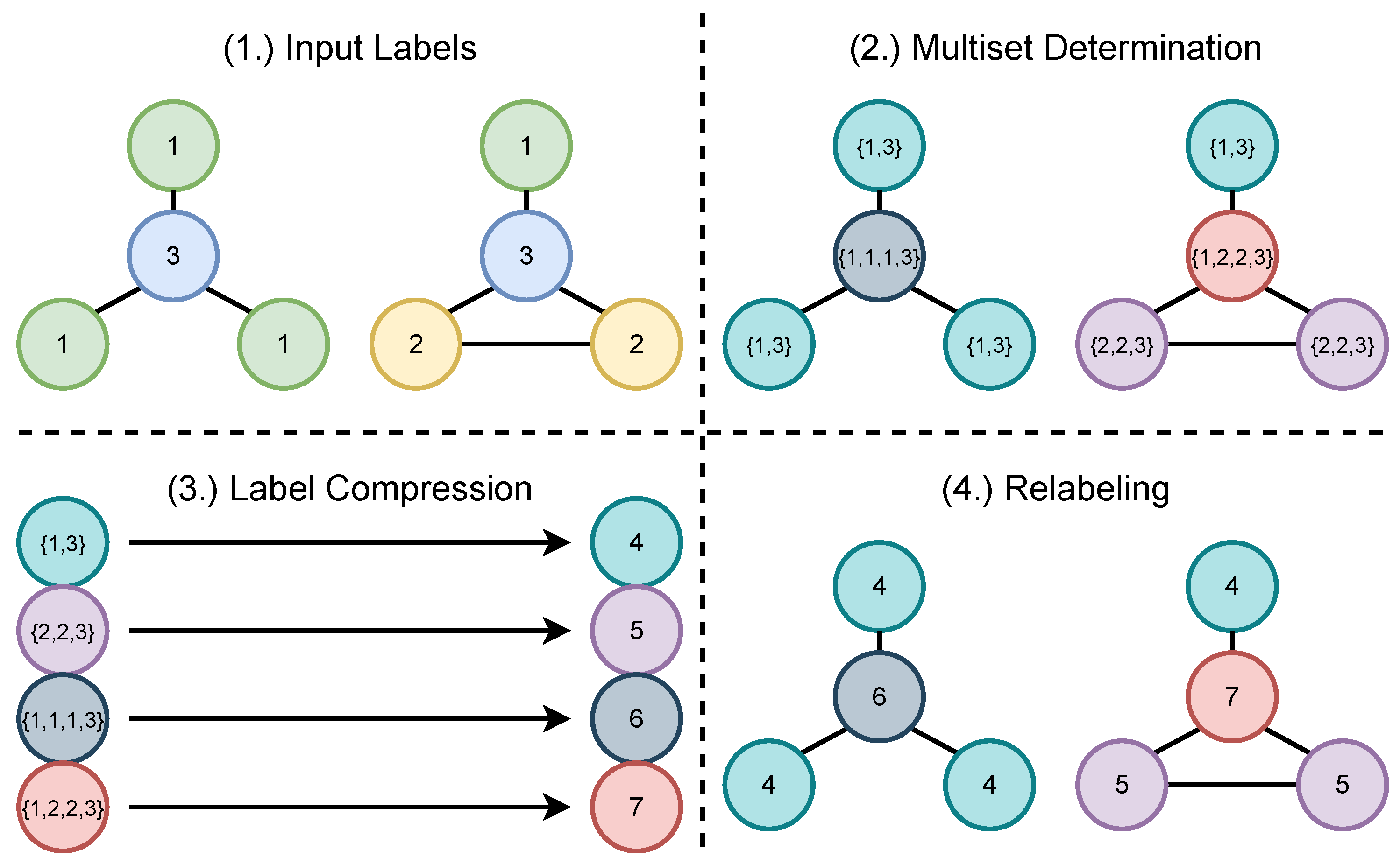
2.2. Expressivity of Weisfeiler–Lehman and $\mathrm{M}\mathrm{A}\mathrm{T}\mathrm{L}\mathrm{A}\mathrm{N}\mathrm{G}$

The classic Weisfeiler–Lehman algorithm (1-WL), also known as color refinement, is shown in Algorithm 1. The algorithm starts with an initial color assignment to each vertex $c_v^0$ according to their degree and proceeds updating the assignment at each iteration.

Algorithm 1 1-WL (Color refinement).

Input:  $G=(V,E)$  1: $c_v^0:=\mathtt{hash}\left(\left\{\left\{d_G\left(v\right)\right\}\right\}\right)\forall v\in V$  2: do  3:     $c_v^{i+1}:=\mathtt{hash}\left(\left\{\{c_u^i:\forall u\in {\mathcal{N}}_G^1\left(v\right)\}\right\}\right)$  4: while$c_v^i\ne c_v^{i-1}$ Output:  $c_v^i:V\mapsto \mathbb{N}$

The update aggregates, for each node v, its color $c_v^i$ and the colors of its neigbors $c_u^i$, then hashes this multi-set of colors, mapping it into a new color to be used in the next iteration $c_v^{i+1}$. The algorithm converges to a stable color assignment, which can be used to test graphs for isomorphism. Note that neighbor aggregation in 1-WL can be understood as a message passing step, with the $\mathtt{hash}$ operation being analogous to Update steps in MP-GNNs.

Two graphs, $G_1$, $G_2$, are not isomorphic if they are distinguishable (that is, their stable color assignments do not match). However, if they are not distinguishable (that is, their stable color assignments match), they are likely to be isomorphic [35]. To reduce the likelihood of false positives when color assignments match, one can consider k-tuples of vertices instead of single vertices, leading to higher order variants of the WL test (denoted k-WL) which assign colors to k-vertex tuples. In this case, $G_1$ and $G_2$ are said to be k-WL equivalent, denoted $G_1{\equiv }_{k-\mathrm{WL}}{G}_2$, if their stable assignments are not distinguishable. For more details on the algorithm, we refer to [14,36]. k-WL tests are more expressive than their $(k-1)$-WL counterparts for $k>2$, with the exception of 2-WL, which is known to be as expressive as the 1-WL color refinement test [10].

Among the various characterizations of k-WL expressivity, the relationship with matrix query languages defined by Matlang [11] has also found applications for graph representation learning [26]. Matlang is a language of operations on matrices, where sentences are formed by sequences of operations. There exists a subset of Matlang—${\mathbf{ML}}_1$—that is as expressive as the 1-WL test. Another subset—${\mathbf{ML}}_2$—is strictly more expressive than the 1-WL test but less expressive than the 3-WL test. Finally, there exists another subset ${\mathbf{ML}}_3$ that is as expressive as the 3-WL test [13]. We provide additional technical details on Matlang and its sub-languages in Appendix E, where we analyze the relation between $\mathrm{I}\mathrm{G}\mathrm{E}\mathrm{L}$ and Matlang.

2.3. Graph Neural Networks beyond 1-WL

Recently, approaches have been proposed for improving the expressivity of MP-GNNs. Here, we focus on subgraph and substructure GNNs, which are most closely related to $\mathrm{I}\mathrm{G}\mathrm{E}\mathrm{L}$. For an overview on augmented message passing methods, see [37] and Appendix I.

k-hop MP-GNNs (k-hop) [16] propagate messages beyond immediate vertex neighbors, effectively using ego network information in the vertex representation. Neighborhood subgraphs are extracted, and message passing occurs on each subgraph, with an exponential cost on the number of hops k both at preprocessing and at each iteration (epoch). In contrast, $\mathrm{I}\mathrm{G}\mathrm{E}\mathrm{L}$ only requires a preprocessing step that can be cached once computed.

Distance encoding GNNs (DE-GNN) [38] also propose to improve MP-GNN by using extra node features by encoding distances to a subset of p nodes. The features obtained by DE-GNN are similar to IGEL when conditioning the subset to size $p=1$ and using a distance encoding function with $k=\alpha$. However, these features are not strictly equivalent to $\mathrm{I}\mathrm{G}\mathrm{E}\mathrm{L}$, as node degrees within the ego network can be smaller than in the full graph.

Graph Substructure networks (GSNs) [19] incorporate topological features by counting local substructures (such as the presence of cliques or cycles). GSNs require expert knowledge on what features are relevant for a given task with modifications to MP-GNN architectures. In contrast, $\mathrm{I}\mathrm{G}\mathrm{E}\mathrm{L}$ reaches comparable performance using a general encoding for ego networks and without altering the original message passing mechanism.

GNNML3 [26] performs message passing in spectral domain with a custom frequency profile. While this approach achieves good performance on graph classification, it requires an expensive preprocessing step for computing the eigendecomposition of the graph Laplacian and $\mathcal{O}\left(k\right)$-order tensors to achieve k-WL expressiveness with cubic time complexity.

More recently, a series of methods formulate the problem of representing vertices or graphs as aggregations over subgraphs. The subgraph information is pooled or introduced during message passing at an additional cost that varies depending on each architecture. Consequently, they require generating the subgraphs (or effectively replicating the nodes of every subgraph of interest) and pay an additional overhead due to the aggregation.

These approaches include identity-aware GNNs (ID-GNNs) [39], which embed each node while incorporating identity information in the GNN and apply rounds of heterogeneous message passing; nested GNNs (NGNNs) [20], which perform a two-level GNN using rooted subgraphs and consider a graph as a bag of subgraphs; GNN-as-Kernel (GNN-AK) [21], which follows a similar idea but introduces additional positional and contextual embeddings during aggregation; equivariant subgraph aggregation networks (ESAN) [22] encode graphs as bags of subgraphs and show that such an encoding can lead to a better expressive power; shortest-path neural networks (SPNNs) [40], which represent nodes by aggregating over sets of neighbors at the same distance; and subgraph union networks (SUN) [23], which unify and generalize previous subgraph GNN architectures and connect them to invariant graph networks [41]. Compared to all these methods, $\mathrm{I}\mathrm{G}\mathrm{E}\mathrm{L}$ only relies on an initial preprocessing step based on distances and degrees without having to run additional message passing iterations or modify the architecture of the GNN.

Interestingly, recent work [42] showed that the implicit encoding of the pairwise distance between nodes plus the degree information which can be extracted via aggregation are fundamental to provide a theoretical justification of ESAN. Furthermore, the work on SUN [23] showed that node-based subgraph GNNs are provably as powerful as the 3-WL test. This result is aligned with recent analyses on the hierarchies of model expressivity [43].

In this work, we directly consider distances and degrees in the ego network, explicitly providing the structural information encoded by more expressive GNN architectures. In contrast to previous work, $\mathrm{I}\mathrm{G}\mathrm{E}\mathrm{L}$ aims to be a minimal yet expressive representation of network structures without learning that is amenable to formal analysis, as shown in Section 4. This connects ego network properties to subgraph GNNs, corroborating the 3-WL upper bound of SUN and the expressivity analysis of ESAN—to which $\mathrm{I}\mathrm{G}\mathrm{E}\mathrm{L}$ is strongly related in its ego networks policy (EGO+). Furthermore, these relationships may explain the comparable empirical performance of $\mathrm{I}\mathrm{G}\mathrm{E}\mathrm{L}$ to the state of the art, as shown in Section 5.

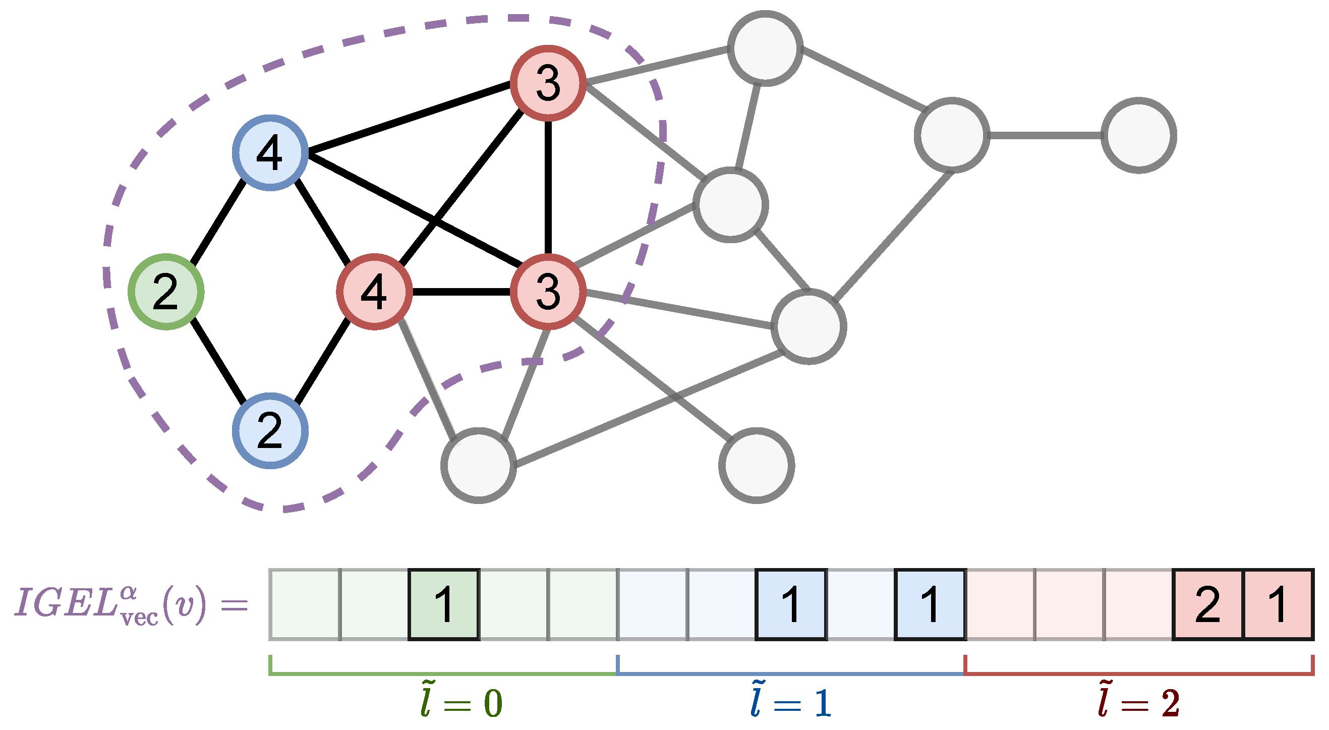
3. Local Ego-Network Encodings

The idea behind the $\mathrm{I}\mathrm{G}\mathrm{E}\mathrm{L}$ encoding is to represent each vertex v by compactly encoding its corresponding ego network ${\mathcal{E}}_v^{\alpha }$ at depth $\alpha$. The choice of encoding consists of a histogram of vertex degrees at distance $d\le \alpha$, for each vertex in ${\mathcal{E}}_v^{\alpha }$. Essentially, $\mathrm{I}\mathrm{G}\mathrm{E}\mathrm{L}$ runs a breadth-first traversal up to depth $\alpha$, counting the number of times the same degree appears at distance $d\le \alpha$. We postulate that such a simple encoding is sufficiently expressive and at the same time computationally tractable to be considered as vertex features.

Figure 1 shows an illustrative example for $\alpha =2$. In this example, the green node is encoded using a (sparse) vector of size $5\times 3=15$, since the maximum degree at depth 2 is 5 and there are three distances considered: $0,1,2$. The ego network contains six nodes, and all (distance, degree) pairs occur once, except for degree 3 at distance 2, which occurs twice. Algorithm 2 describes the steps to produce the $\mathrm{I}\mathrm{G}\mathrm{E}\mathrm{L}$ encoding iteratively.

Algorithm 2 $\mathrm{I}\mathrm{G}\mathrm{E}\mathrm{L}$ Encoding.

Input:  $G=(V,E),\alpha :\mathbb{N}$  1: $e_v^0:=\left\{\left\{(0,d_G\left(v\right))\right\}\right\}\forall v\in V$  2: for> $i:=1$; $i+=1$ until $i=\alpha$do  3:     $e_v^i:=\bigcup (e_v^{i-1},\left\{\{(i,d_{{\mathcal{E}}_G^{\alpha }\left(v\right)}\left(u\right))\forall u\in {\mathcal{N}}_G^{\alpha }\left(v\right)|l_G(u,v)=i\}\right\})$  4: end for Output:  $e_v^{\alpha }:V\mapsto \left\{\left\{(\mathbb{N},\mathbb{N})\right\}\right\}$

Similarly to 1-WL, information of the neighbors of each vertex is aggregated at each iteration. However, 1-WL does not preserve distance information in the encoding due to the hashing step. Instead of hashing the degrees into equivalence classes, $\mathrm{I}\mathrm{G}\mathrm{E}\mathrm{L}$ keeps track of the distance at which a degree is found, generating a more expressive encoding.

The cost of such additional expressiveness is a computational complexity that grows exponentially in the number of iterations. More precisely, the time complexity follows $\mathcal{O}(n·min(m,{\left(d_{\mathtt{max}}\right)}^{\alpha }))$, with $\mathcal{O}(n·m)$ when $\alpha \ge \mathtt{diam}\left(G\right)$. In Appendix F, we provide a possible breadth-first search (BFS) implementation that is embarrassingly parallel and thus can be computed over p processors following $\mathcal{O}(n·min(m,{\left(d_{\mathtt{max}}\right)}^{\alpha })/p)$ time complexity.

The encoding produced by Algorithm 1 can be described as a multi-set of path length and degree pairs $(\tilde{l},\tilde{d})$ in the $\alpha$-depth ego graph of v, ${\mathcal{E}}_v^{\alpha }$:

$$\begin{array}{c}\hfill e_v^{\alpha }=\left\{\right\{(l_{{\mathcal{E}}_v^{\alpha }}(u,v),d_{{\mathcal{E}}_v^{\alpha }}\left(u\right){\displaystyle )}|\forall u\in {\mathcal{N}}_G^{\alpha }\left(v\right)\left\}\right\},\end{array}$$

(4)

which also results in exponential space complexity. However, $e_v^{\alpha }$ can be represented as a (sparse) vector $\mathrm{I}\mathrm{G}\mathrm{E}{\mathrm{L}}_{\mathtt{vec}}^{\alpha }\left(v\right)$, where the i-th index contains the frequency of path length and degree pairs $(\tilde{l},\tilde{d})$, as shown in Figure 1:

$$\begin{array}{c}\hfill \mathrm{I}\mathrm{G}\mathrm{E}{\mathrm{L}}_{\mathtt{vec}}^{\alpha }{\left(v\right)}_i=\left|\{\{(\tilde{l},\tilde{d})\in e_v^{\alpha }\mathrm{s}.\mathrm{t}.f(\tilde{l},\tilde{d})=i\}\}\right|,\end{array}$$

(5)

which has linear space complexity $\mathcal{O}(\alpha ·n·d_{\mathtt{max}})$, conservatively assuming every node requires $d_{\mathtt{max}}$ parameters at every $\alpha$ depth from the center of the ego network, where $d_{\mathtt{max}}=\mathcal{O}\left(n\right)$ in the worst case when a vertex is fully connected. Note that in practice, we may normalize raw counts by, e.g., applying log1p-normalization, and for real-world graphs, $d_{\mathtt{max}}\ll n$, where the probability of larger degrees often decays exponentially [44]). Finally, complexity can be further reduced by making use of sparse vector implementations.

We finish this section with two remarks. First, the produced encodings can differ only for values of $\alpha <\mathtt{diam}\left(G\right)$, since otherwise the ego network is the same for all nodes, ${\mathcal{E}}_v^{\alpha }={\mathcal{E}}_v^{\alpha +1}=G,\forall v$, and thus the resulting encodings, i.e., $e_v^{\alpha }=e_v^{\alpha +1},$ for $\alpha \ge \mathtt{diam}\left(G\right)$. Second, the sparse formulation in Equation (5) can be understood as an inductive analogue of Weisfeiler–Lehman graph kernels [45], as we explore in Appendix B.

4. Which Graphs Are $\mathrm{I}\mathrm{G}\mathrm{E}\mathrm{L}$-Distinguishable?

We now present results about the expressive power of $\mathrm{I}\mathrm{G}\mathrm{E}\mathrm{L}$, extending previous preliminary results on 1-WL that had been presented in [46]. We discuss the increased expressivity of $\mathrm{I}\mathrm{G}\mathrm{E}\mathrm{L}$ with respect to 1-WL, and identify upper-bounds on the expressivity on graphs that are also indistinguishable under Matlang and the 3-WL test. We assess expressivity by studying whether two graphs can be distinguished by comparing the encodings obtained by the k-WL test and the $\mathrm{I}\mathrm{G}\mathrm{E}\mathrm{L}$ encodings for a given value of $\alpha$. Similarly to the definition of k-WL equivalence, we say that $G_1=(V_1,E_1)$ and $G_2=(V_1,E_1)$ are $\mathrm{I}\mathrm{G}\mathrm{E}\mathrm{L}$-equivalent if the sorted multi-set of node representations is the same for $G_1$ and $G_2$:

$$\begin{array}{c}{G}_1{\equiv }_{\mathrm{I}\mathrm{G}\mathrm{E}\mathrm{L}}^{\alpha }{G}_2\iff \left\{\{e_{v_1}^{\alpha }:\forall v_1\in V_1\}\right\}=\left\{\{e_{v_2}^{\alpha }:\forall v_2\in V_2\}\right\}.\end{array}$$

4.1. Distinguishability on 1-WL Equivalent Graphs

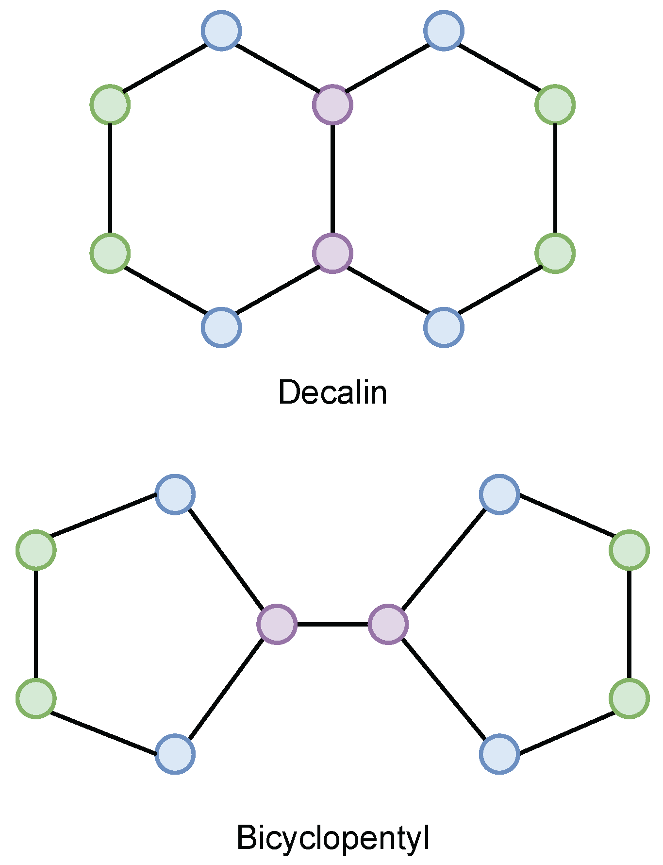
We first show $\mathrm{I}\mathrm{G}\mathrm{E}\mathrm{L}$ is more powerful than 1-WL, following Lemmas 1 and 2:

Lemma 1.

$\mathrm{I}\mathrm{G}\mathrm{E}\mathrm{L}$ is at least as expressive as 1-WL. For two graphs, $G_1$, $G_2$, which are distinguished by 1-WL in k iterations ($G_1{\cancel{\equiv }}_{1-\mathrm{WL}}{G}_2$) it also holds that $G_1{\cancel{\equiv }}_{\mathrm{I}\mathrm{G}\mathrm{E}\mathrm{L}}^{\alpha }{G}_2$ for $\alpha =k+1$. If $\mathrm{I}\mathrm{G}\mathrm{E}\mathrm{L}$ does not distinguish two graphs $G_1^{\prime }$ and $G_2^{\prime }$, 1-WL also does not distinguish them: $G_1^{\prime }{\equiv }_{\mathrm{I}\mathrm{G}\mathrm{E}\mathrm{L}}^{\alpha }{G}_2^{\prime }\Rightarrow G_1^{\prime }{\equiv }_{1-WL}{G}_2^{\prime }$.

Lemma 2.

There exist at least two non-isomorphic graphs, $G_1,G_2$, that $\mathrm{I}\mathrm{G}\mathrm{E}\mathrm{L}$ can distinguish but that 1-WL cannot distinguish; i.e., $G_1{\cancel{\equiv }}_{\mathrm{I}\mathrm{G}\mathrm{E}\mathrm{L}}^{\alpha }{G}_2$ while $G_1{\equiv }_{1-WL}{G}_2$.

First, we formally prove Lemma 1, i.e., that $\mathrm{I}\mathrm{G}\mathrm{E}\mathrm{L}$ is at least as expressive as 1-WL. For this, we consider a variant of 1-WL which removes the hashing step. This modification can only increase the expressive power of 1-WL and makes it possible to directly compare such (possibly more expressive) 1-WL encodings with the encodings generated by $\mathrm{I}\mathrm{G}\mathrm{E}\mathrm{L}$. Intuitively, after k color refinement iterations, 1-WL considers nodes at k hops from each node, which is equivalent to running $\mathrm{I}\mathrm{G}\mathrm{E}\mathrm{L}$ with $\alpha =k+1$, i.e., using ego networks that include information of all nodes that 1-WL would visit.

Proof of Lemma 1.

For convenience, let $c_v^{i+1}=\left\{\{c_v^i;c_u^i\forall u\in {\mathcal{N}}_G^1\left(v\right)|u\ne v\}\right\}$ be a recursive definition of Algorithm 1 where hashing is removed and $c_v^0=\left\{\left\{d_G\left(v\right)\right\}\right\}$. Since the hash is no longer computed, the nested multi-sets contain strictly the same or more information as in the traditional 1-WL algorithm.

For $\mathrm{I}\mathrm{G}\mathrm{E}\mathrm{L}$ to be less expressive than 1-WL, it must hold that there exist two graphs $G_1=(V_1,E_1)$ and $G_2=(V_2,E_2)$ such that $G_1{\cancel{\equiv }}_{1-\mathrm{WL}}{G}_2$ while $G_1{\equiv }_{\mathrm{I}\mathrm{G}\mathrm{E}\mathrm{L}}^{\alpha }{G}_2$.

Let k be the minimum number of color refinement iterations such that $\exists v_1\in V_1$ and $\forall v_2\in V_2,c_{v_1}^k\ne c_{v_2}^k$. We define an equally or more expressive variant of the 1-WL test 1-WL^* where hashing is removed, such that $c_{v_1}^k=\{\{\{\{...\{\{d_G\left(v_1\right)\}\},\{\{d_G\left(u\right)\forall u\in {\mathcal{N}}_{G_1}^1\left(v_1\right)\}\}...\}\}\}\}$, nested up to depth k. To avoid nesting, the multi-set of nested degree multi-sets can be rewritten as the union of degree multi-sets by introducing an indicator variable for the iteration number where a degree is found:

$$\begin{array}{cc}\hfill c_{v_1}^k=& \left\{\right\{(0,d_G\left(v_1\right))\left\}\right\}\bigcup \hfill \\ \hfill & \left\{\right\{(1,d_G\left(v_1\right));(1,d_G\left(u\right))\forall u\in {\mathcal{N}}_G^1\left(v_1\right)\left\}\right\}\bigcup \hfill \\ \hfill & \left\{\left\{(2,d_G\left(v_1\right));(2,d_G\left(u\right))\forall u\in {\mathcal{N}}_G^1\left(v_1\right);(2,d_G\left(w\right))\forall w\in {\mathcal{N}}_G^1\left(u\right)\right\}\right\}\bigcup ...\hfill \end{array}$$

At each step i, we introduce information about nodes up to distance i of $v_1$. Furthermore, by construction, nodes will be visited on every subsequent iteration—i.e., for $c_{v_1}^2$, we will observe $(2,d_G\left(v_1\right))$ exactly $d_G\left(v_1\right)+1$ times, as all its $d_G\left(v_1\right)$ neighbors $u\in {\mathcal{N}}_G^1\left(v\right)$ encode the degree of $v_1$ in $c_u^1$. The flattened representation provided by 1-WL^* is still equally or more expressive than 1-WL, as it removes hashing and keeps track of the iteration at which a degree is found.

Let $\mathrm{I}\mathrm{G}\mathrm{E}\mathrm{L}-\mathrm{W}$ be a less expressive version of $\mathrm{I}\mathrm{G}\mathrm{E}\mathrm{L}$ that does not include edges between nodes at $k+1$ hops of the ego network root. Now, consider the case in which $c_{v_1}^k\ne c_{v_2}^k$ from 1-WL^*, and let $\alpha =k+1$ so that $\mathrm{I}\mathrm{G}\mathrm{E}\mathrm{L}-\mathrm{W}$ considers degrees by counting edges found at k to $k+1$ hops of $v_1$ and $v_2$. Assume that $G_1{\equiv }_{\mathrm{I}\mathrm{G}\mathrm{E}\mathrm{L}-\mathrm{W}}^{\alpha }{G}_2$. By construction, this means that $\left\{\{e_{v_1}^{\alpha }:\forall v_1\in V_1\}\right\}=\left\{\{e_{v_2}^{\alpha }:\forall v_2\in V_2\}\right\}$. This implies that all degrees and iteration counts match as per the distance indicator variable at which the degrees are found, so $c_{v_1}^k=c_{v_2}^k$ which contradicts the assumption $c_{v_1}^k\ne c_{v_2}^k$ and therefore implies that also $G_1{\equiv }_{1-\mathrm{WL}*}{G}_2$. Thus, $G_1{\equiv }_{\mathrm{I}\mathrm{G}\mathrm{E}\mathrm{L}-\mathrm{W}}^{\alpha }{G}_2\Rightarrow G_1{\equiv }_{1-\mathrm{WL}*}{G}_2$ for $\alpha =k+1$ and also $G_1\neg {\equiv }_{1-\mathrm{WL}*}{G}_2\Rightarrow G_1\neg {\equiv }_{\mathrm{I}\mathrm{G}\mathrm{E}\mathrm{L}-\mathrm{W}}^{\alpha }{G}_2$. Therefore, by extension $\mathrm{I}\mathrm{G}\mathrm{E}\mathrm{L}$ is at least as expressive as 1-WL.    □

To prove Lemma 2, we show graphs that $\mathrm{I}\mathrm{G}\mathrm{E}\mathrm{L}$ can distinguish despite being undistinguishable by 1-WL and the Matlang sub-languages ${\mathbf{ML}}_1$ and ${\mathbf{ML}}_2$. In Section 4.1.1, we provide an example where $\mathrm{I}\mathrm{G}\mathrm{E}\mathrm{L}$ distinguishes 1-WL/${\mathbf{ML}}_1$ equivalent graphs, while Section 4.1.2 shows that $\mathrm{I}\mathrm{G}\mathrm{E}\mathrm{L}$ also distinguishes graphs that are known to be distinguishable in the strictly more expressive ${\mathbf{ML}}_2$ language.

4.1.1. ${\mathbf{ML}}_1$/1-WL Expressivity: Decalin and Bicyclopentyl

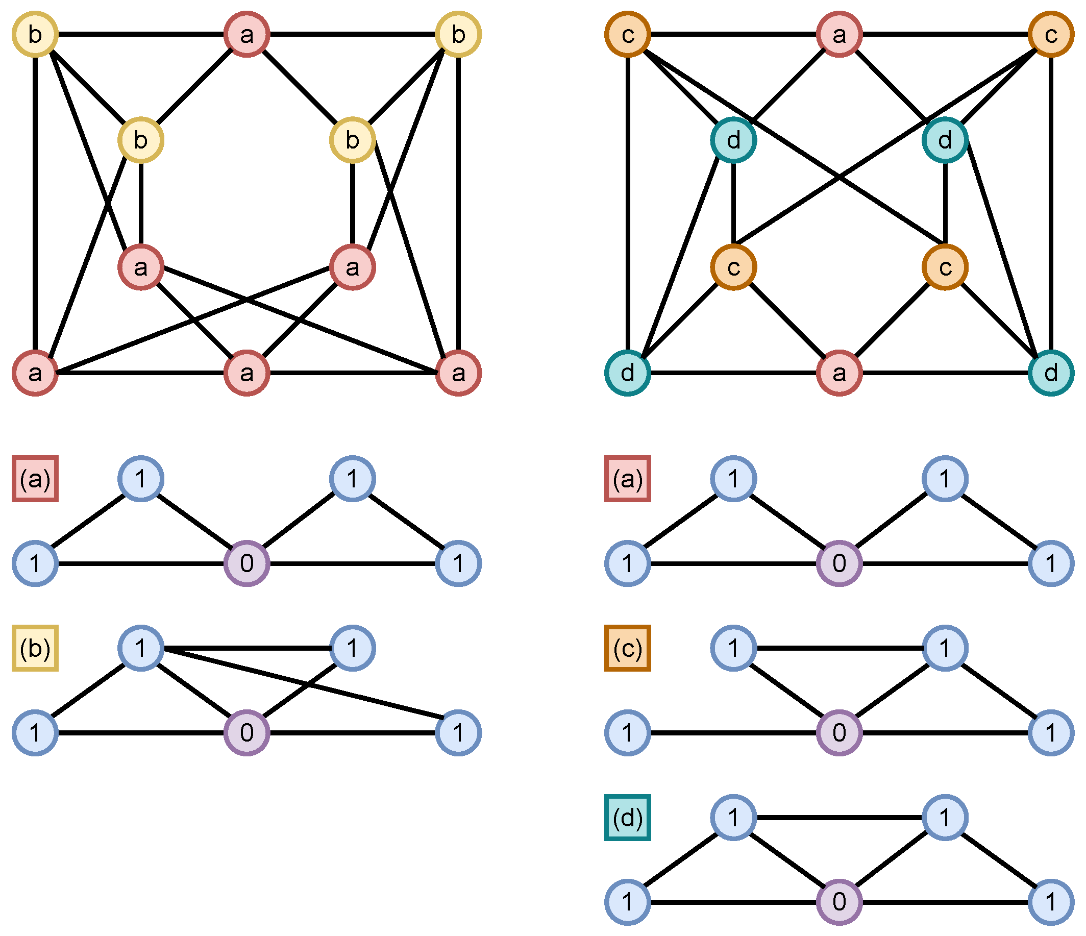
Decalin and Bycyclopentyl (in Figure 2) are two molecules whose graph representations are not distinguishable by 1-WL despite their simplicity. The graphs are non-isomorphic, but 1-WL identifies 3 equivalence classes in both graphs: central nodes with degree 3 (purple), their neighbors (blue), and peripheral nodes farthest from the center (green).

Figure 2 shows the resulting $\mathrm{I}\mathrm{G}\mathrm{E}\mathrm{L}$ encoding for the central node (in purple) using $\alpha =1$ (top) and $\alpha =2$ (bottom). For $\alpha =1$, the encoding field of $\mathrm{I}\mathrm{G}\mathrm{E}\mathrm{L}$ is too narrow to identify substructures that distinguish the two graphs (Figure 3, top). However, for $\alpha =2$ the representations of central nodes differ between the two graphs (Figure 3, bottom). In this example, any value of $\alpha \ge 2$ can distinguish between the graphs.

4.1.2. ${\mathbf{ML}}_2$ Expressivity: Cospectral 4-Regular Graphs

$\mathrm{I}\mathrm{G}\mathrm{E}\mathrm{L}$ can also distinguish ${\mathbf{ML}}_2$-equivalent graphs. Recall that ${\mathbf{ML}}_2$ is strictly more expressive than 1-WL, as described in Section 2.2. It is known that d-regular graphs of the same cardinality are indistinguishable by the 1-WL test in Algorithm 1 and that co-spectral graphs cannot be distinguished in ${\mathbf{ML}}_2$:

Definition 1.

$G=(V,E)$ is d-regular with $d\in \mathbb{N}$ if $\forall v\in V,d_G\left(v\right)=d$.

Remark 1.

For any pair of n-vertex d-regular graphs $G_1=(V_1,E_1)$ and $G_2=(V_2,E_2)$, $G_1{\equiv }_{1-\mathrm{WL}}{G}_2$ (see [10], Example 3.5.2, p. 81).

Definition 2.

Two graphs $G_1=(V_1,E_1)$ and $G_2=(V_2,E_2)$ are co-spectral if their adjacency matrices have the same multi-set of eigenvalues.

Remark 2.

For any pair of n-vertex co-spectral graphs $G_1=(V_1,E_1)$ and $G_2=(V_2,E_2)$, $G_1{\equiv }_{{\mathit{M}\mathit{L}}_2}{G}_2$ (see [13], Proposition 5.1).

In contrast to 1-WL, we can find examples of non-isomorphic d-regular graphs that $\mathrm{I}\mathrm{G}\mathrm{E}\mathrm{L}$ can distinguish, as the generated encodings will differ for any pair of graphs whose sets of sorted degree sequences do not match at any path length less than $\alpha$. Furthermore, we can find examples of co-spectral graphs that can be distinguished by $\mathrm{I}\mathrm{G}\mathrm{E}\mathrm{L}$ encodings. In both cases, the intuition is that the ego network encoding generated by $\mathrm{I}\mathrm{G}\mathrm{E}\mathrm{L}$ discards the edges that connect nodes beyond the subgraph. Consequently, the generated encoding will depend on the actual connectivity at the boundary of the ego network and provide $\mathrm{I}\mathrm{G}\mathrm{E}\mathrm{L}$ with increased expressivity compared to other methods.

Figure 4 shows two co-spectral 4-regular graphs taken from [47], and the structures obtained using $\mathrm{I}\mathrm{G}\mathrm{E}\mathrm{L}$ encodings with $\alpha =1$ on each graph. The 1-WL test assigns a single color to all nodes and stabilizes after one iteration. Likewise, any ${\mathbf{ML}}_2$ sentences executed as operations on the adjacency matrices of both graphs produce equal results. However, $\mathrm{I}\mathrm{G}\mathrm{E}\mathrm{L}$ identifies four different structures (denoted a, b, c, d). Since the $\mathrm{I}\mathrm{G}\mathrm{E}\mathrm{L}$ encodings between both graphs do not match, they are distinguishable. This is the case for any value of $\alpha \ge 1$.

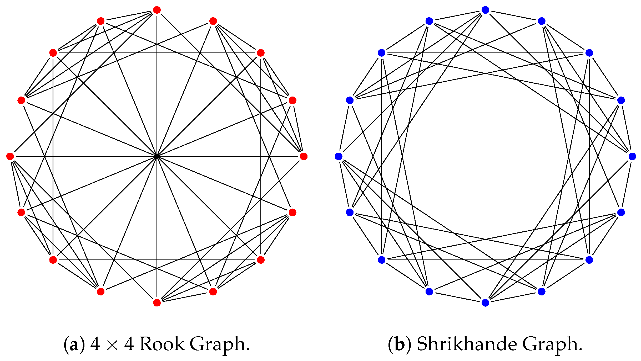
4.2. Indistinguishability on Strongly Regular Graphs

We identify an upper bound on the expressive power of $\mathrm{I}\mathrm{G}\mathrm{E}\mathrm{L}$: non-isomorphic Strongly Regular Graphs with equal parameters. In this case, two non-isomorphic graphs are not indistinguishable by $\mathrm{I}\mathrm{G}\mathrm{E}\mathrm{L}$.

Definition 3.

A n-vertex d-regular graph is strongly regular—denoted $\mathtt{SRG}(n,d,\lambda ,\gamma )$—if all adjacent vertices have λ vertices in common and all non-adjacent vertices have γ vertices in common.

Remark 3.

For any $G=\mathtt{SRG}(n,d,\lambda ,\gamma )$, $\mathtt{diam}\left(G\right)\le 2$ [48].

Theorem 1.

$\mathrm{I}\mathrm{G}\mathrm{E}\mathrm{L}$ cannot distinguish two SRGs when n, d, and λ are the same, and between any value of γ (equal or not).

Formally, given $G_1=\mathtt{SRG}(n_1,d_1,{\lambda }_1,{\gamma }_1)$, $G_2=\mathtt{SRG}(n_2,d_2,{\lambda }_2,{\gamma }_2)$:

—

$G_1{\equiv }_{Igel}^1{G}_2\iff n_1=n_2\wedge d_1=d_2\wedge {\lambda }_1={\lambda }_2$;

—

$G_1{\equiv }_{\mathrm{I}\mathrm{G}\mathrm{E}\mathrm{L}}^2{G}_2\iff n_1=n_2\wedge d_1=d_2$;

—

no values of γ can be distinguished by ${\equiv }_{\mathrm{I}\mathrm{G}\mathrm{E}\mathrm{L}}^1$ or ${\equiv }_{\mathrm{I}\mathrm{G}\mathrm{E}\mathrm{L}}^2$.

Proof. 

Recall that for any graph G, $\mathrm{I}\mathrm{G}\mathrm{E}\mathrm{L}$ encodings are equal for all $\alpha \ge \mathtt{diam}\left(G\right)$ and per Remark 3, SRGs have diameters of two or less. Let $G=\mathtt{SRG}(n,d,\lambda ,\gamma )$, only $\alpha \in \{1,2\}$ produce different encodings for nodes of G. By construction, $\forall v$ in G, v has encoding $e_v^{\alpha }$, so the encoding of G is $e_G^{\alpha }={\left\{\left\{e_v^{\alpha }\right\}\right\}}^n$. Furthermore, ${\left\{\left\{e_v^1\right\}\right\}}^n$ only encodes n, d, and $\lambda$, and ${\left\{\left\{e_v^2\right\}\right\}}^n$ only encodes n and d by expanding $e_v^{\alpha }$ in Algorithm 2:

-

Let $\alpha =1$: $\forall v\in V,{\mathcal{E}}_v^1=(V^{\prime },E^{\prime })s.t.V^{\prime }={\mathcal{N}}_G^1\left(v\right)$. Since G is d-regular, v is the center of ${\mathcal{E}}_v^1$, and has d-neighbors. By definition, d neighbors of v have $\lambda$ shared neighbors with v each, plus an edge with v, and ${\mathcal{E}}_v^1$ does not include $\gamma$ edges beyond its neighbors. Thus, for SRGs $G_1,G_2$ where $n_1=n_2$, $d_1=d_2$, and ${\lambda }_1={\lambda }_2$, $e_{G_1}^1=e_{G_2}^1={\left\{\left\{e_v^1\right\}\right\}}^n$ where

$$e_v^1=\left\{\right\{(0,d)\left\}\right\}\bigcup {{\displaystyle \left\{\right\{(}1,\lambda +1{\displaystyle )\}\}}}^d.$$

-

Let $\alpha =2$: $\forall v\in V,{\mathcal{E}}_v^2=G$ as $\forall u\in V,u\in {\mathcal{N}}_G^2\left(v\right)$ when $\mathtt{diam}\left(G\right)\le 2$. G is d-regular, so $\forall v\in V,d=d_{{\mathcal{E}}_v^2}\left(v\right)=d_G\left(v\right)$. Thus, for any SRGs $G_1,G_2$ s.t. $n_1=n_2$ and $d_1=d_2$, $e_{G_1}^2=e_{G_1}^2={\left\{\left\{e_v^2\right\}\right\}}^n$ where

$$\begin{array}{c}{e}_v^2=\left\{\right\{(0,d)\left\}\right\}\bigcup {\left\{\right\{(1,d)\left\}\right\}}^d\bigcup {\left\{\right\{(2,d)\left\}\right\}}^{n-d-1}\end{array}$$

Thus, $\mathrm{I}\mathrm{G}\mathrm{E}\mathrm{L}$ with $\alpha \in \{1,2\}$ can only distinguish between different values of n, d and $\lambda$.    □

4.3. Expressivity Implications

As expected from Theorem 1, $\mathrm{I}\mathrm{G}\mathrm{E}\mathrm{L}$ cannot distinguish the Shrikhande and $4\times 4$ Rook graphs (shown in Figure 5), which are known to be ${\mathbf{ML}}_3$-equivalent graphs [26,49] with $\mathtt{SRG}(16,6,2,2)$ parameters despite not being isomorphic.

Our findings show that $\mathrm{I}\mathrm{G}\mathrm{E}\mathrm{L}$ is a powerful permutation-equivariant representation (see Lemma A1), capable of distinguishing 1-WL equivalent graphs such as Figure 4—which as cospectral graphs are known to be expressable in strictly more powerful Matlang sub-languages than 1-WL [13]. Furthermore, in Appendix D, we connect $\mathrm{I}\mathrm{G}\mathrm{E}\mathrm{L}$ to SPNNs [40] and show that $\mathrm{I}\mathrm{G}\mathrm{E}\mathrm{L}$ is strictly more expressive than SPNNs on unattributed graphs. Finally, we note that the upper bound on strongly regular graphs is a hard ceiling on expressivity since SRGs are commonly known to be indistinguishable by 3-WL [14,21,23,43,49].

$\mathrm{I}\mathrm{G}\mathrm{E}\mathrm{L}$ formally reaches an expressivity upper bound on SRGs, distinguishing SRGs with different values of n, d, and $\lambda$. These results are similar with subgraph methods implemented within MP-GNN architectures, such as nested GNNs [20] and GNN-AK [21], which are known to be not less powerful than 3-WL, and the ESAN framework when leveraging ego networks with root-node flags as a subgraph sampling policy (EGO+), which is as powerful as 3-WL on SRGs [22]. However, in contrast to these methods, $\mathrm{I}\mathrm{G}\mathrm{E}\mathrm{L}$ cannot distinguish graphs with different values of $\gamma$. Furthermore, in Section 5, we study $\mathrm{I}\mathrm{G}\mathrm{E}\mathrm{L}$ in a series of empirical tasks, finding that the expressivity difference that $\mathrm{I}\mathrm{G}\mathrm{E}\mathrm{L}$ exhibits on SRGs does not have significant implications in downstream tasks.

Summarizing, $\mathrm{I}\mathrm{G}\mathrm{E}\mathrm{L}$ distinguishes non-isomorphic graphs that are undistinguishable by the 1-WL test. Furthermore, Lemma 2 shows that $\mathrm{I}\mathrm{G}\mathrm{E}\mathrm{L}$ can distinguish any graphs that 1-WL can distinguish. We derive a precise expressivity upper bound for $\mathrm{I}\mathrm{G}\mathrm{E}\mathrm{L}$ on SRGs, showing that $\mathrm{I}\mathrm{G}\mathrm{E}\mathrm{L}$ cannot distinguish SRGs with equal parameters or between values of $\gamma$. Overall, the expressive power of $\mathrm{I}\mathrm{G}\mathrm{E}\mathrm{L}$ on SRGs is similar to other state-of-the-art methods, including k-hop GNNs [16], GSNs [19], NGNNs [20], GNN-AK [21], and ESAN [22].

5. Empirical Validation

We evaluate $\mathrm{I}\mathrm{G}\mathrm{E}\mathrm{L}$ as a sparse local ego network encoding following Equation (5), extending vertex/edge attributes on six experimental tasks: graph classification, graph isomorphism detection, graphlet counting, graph regression, link prediction, and vertex classification. With our experiments, we seek to evaluate the following empirical questions:

Q1. 

Does $\mathrm{I}\mathrm{G}\mathrm{E}\mathrm{L}$ improve MP-GNN performance on standard graph-level tasks?

Q2. 

Can we empirically validate our results on the expressive power of $\mathrm{I}\mathrm{G}\mathrm{E}\mathrm{L}$ compared to 1-WL?

Q3. 

Are $\mathrm{I}\mathrm{G}\mathrm{E}\mathrm{L}$ encodings appropriate features to learn on unattributed graphs?

Q4. 

How do GNN models compare with more traditional neural network models when they are enriched with $\mathrm{I}\mathrm{G}\mathrm{E}\mathrm{L}$ features?

5.1. Overview of the Experiments

For graph classification, isomorphism detection, and graphlet counting, we reproduce the benchmark proposed by [26] on eight graph data sets. For each task and data set, we introduce $\mathrm{I}\mathrm{G}\mathrm{E}\mathrm{L}$ as vertex/edge attributes, and compare the performance of including or excluding $\mathrm{I}\mathrm{G}\mathrm{E}\mathrm{L}$ on several GNN architectures—including linear and MLP baselines (without message passing), GCNs [31], GATs [33], GINs [8], Chebnets [30], and GNNML3 [26]. We measure whether $\mathrm{I}\mathrm{G}\mathrm{E}\mathrm{L}$ improves inductive MP-GNN performance while validating our theoretical expressivity analysis (Q1 and Q2). We also evaluate on the Zinc-12K and Pattern data sets from benchmarking GNNs [50] to test $\mathrm{I}\mathrm{G}\mathrm{E}\mathrm{L}$ on larger, real-world data sets.

For link prediction, we experiment on two unattributed social network graphs. We train self-supervised embeddings on $\mathrm{I}\mathrm{G}\mathrm{E}\mathrm{L}$ encodings and compare them against standard transductive vertex embeddings. Transductive methods require that all nodes in the graph are known at training and inference time, while inductive methods can be applied to unseen nodes, edges, and graphs. Inductive methods may be applied in transductive settings but not vice-versa. Since $\mathrm{I}\mathrm{G}\mathrm{E}\mathrm{L}$ is label and permutation invariant, its output is an inductive representation. We detail the self-supervised embedding approach in Appendix H. We compare our results against strong vertex embedding models, namely DeepWalk [51] and Node2Vec [52], seeking to validate $\mathrm{I}\mathrm{G}\mathrm{E}\mathrm{L}$ as a theoretically grounded structural feature extractor in unattributed graphs (Q3).

For vertex classification, we train using $\mathrm{I}\mathrm{G}\mathrm{E}\mathrm{L}$ encodings and vertex attributes as inputs on DNN models without message passing on an inductive protein-to-protein interaction (PPI) multi-label classification problem. We evaluate the impact of introducing $\mathrm{I}\mathrm{G}\mathrm{E}\mathrm{L}$ on top of vertex attributes and compare the performance of $\mathrm{I}\mathrm{G}\mathrm{E}\mathrm{L}$-inclusive models with MP-GNNs (Q4).

5.2. Experimental Methodology

On graph-level tasks, we introduce $\mathrm{I}\mathrm{G}\mathrm{E}\mathrm{L}$ encodings concatenated to existing vertex features, and also introduce $\mathrm{I}\mathrm{G}\mathrm{E}\mathrm{L}$ as edge-level features representing an edge as the element-wise product of node-level $\mathrm{I}\mathrm{G}\mathrm{E}\mathrm{L}$ encodings at each end of the edge into the best performing model configurations found by [26] without any hyper-parameter tuning (e.g., number of layers, hidden units, choice pooling and activation functions). We evaluate performance differences with and without $\mathrm{I}\mathrm{G}\mathrm{E}\mathrm{L}$ on each task, data set and model on 10 independent runs, measuring statistical significance of the differences through paired t-tests. On benchmark data sets, we reuse the best reported GIN-AK⁺ baseline from [21] and simply introduce $\mathrm{I}\mathrm{G}\mathrm{E}\mathrm{L}$ as additional node features with $\alpha \in \{1,2\}$, with no hyper-parameter changes.

On vertex and edge-level tasks, we report best performing configurations after hyper-parameter search. Each configuration is evaluated on five independent runs. Our results are compared against strong standard baselines from the literature, and we provide a breakdown of the best-performing hyper-parameters found in Appendix A.

5.3. Results and Notation

The following formatting denotes significant (as per paired t-tests) positive (in bold), negative (in italic), and insignificant differences (no formatting) after introducing $\mathrm{I}\mathrm{G}\mathrm{E}\mathrm{L}$, with the best results per task/data set underlined.

5.4. Graph Classification: TU Graphs

Table 1. Per-model classification accuracy metrics on TU data sets. Each cell shows the average accuracy of the model and data set in that row and column, with $\mathrm{I}\mathrm{G}\mathrm{E}\mathrm{L}$ (left) and without $\mathrm{I}\mathrm{G}\mathrm{E}\mathrm{L}$ (right).

Model	Enzymes	Mutag	Proteins	PTC
MLP	41.10 > 26.18⋄	87.61 > 84.61⋄	75.43 ~ 75.01	64.59 > 62.79 ⋄
GCN	54.48 > 48.60⋄	89.61 > 85.42⋄	75.67 > 74.50 *	65.76 ~ 65.21
GAT	54.88 ~ 54.95	90.00 > 86.14⋄	73.44 > 70.51⋄	66.29 ~ 66.29
GIN	54.77 > 53.44 *	89.56 ~ 88.33	73.32 > 72.05⋄	61.44 ~ 60.21
Chebnet	61.88 ~ 62.23	91.44 > 88.33⋄	74.30 > 66.94⋄	64.79 ~ 63.87
GNNML3	61.42 < 62.79⋄	92.50 > 91.47 *	75.54 > 62.32⋄	64.26 < 66.10⋄

shows graph classification results for TU molecule data sets [28]. In each data set, nodes represent atoms and edges represent their atomic bonds. The graphs contain no edge features while, node features are a one-hot encoded vector of the atom represented by that node. We evaluate differences in mean accuracies with and without $\mathrm{I}\mathrm{G}\mathrm{E}\mathrm{L}$ through paired t-tests, denoting significance intervals of $p<0.01$ as ^* and $p<0.0001$ as ^⋄.

Our results show that $\mathrm{I}\mathrm{G}\mathrm{E}\mathrm{L}$ in the Mutag and Proteins data sets improves the performance of all MP-GNN models, including GNNML3, contributing to answer Q1. By introducing $\mathrm{I}\mathrm{G}\mathrm{E}\mathrm{L}$ in those data sets, MP-GNN models reach similar performance to GNNML3. Introducing $\mathrm{I}\mathrm{G}\mathrm{E}\mathrm{L}$ achieves this at $\mathcal{O}(n·min(m,{\left(d_{\mathtt{max}}\right)}^{\alpha }))$ preprocessing costs compared to $\mathcal{O}\left(n^3\right)$ worst-case eigen-decomposition costs associated with GNNML3’s spectral supports.

Additionally, since $\mathrm{I}\mathrm{G}\mathrm{E}\mathrm{L}$ is an inductive method, the worst-case $\mathcal{O}(n·{\left(d_{\mathtt{max}}\right)}^{\alpha })$ when $\alpha <\mathtt{diam}\left(G\right)$ cost is only required when the graph is first processed. Afterwards, encodings can be reused, recomputing them for nodes neighboring new nodes or updated edges as given by $\alpha$. This contrasts with GNNML3’s spectral supports, which are computed on the adjacency matrix and would require a full recalculation when nodes or edges change.

On the Enzymes and PTC data sets, results are mixed: for all models other than GNNML3, $\mathrm{I}\mathrm{G}\mathrm{E}\mathrm{L}$ either significantly improves accuracy (on MLPNet, GCN, and GIN on Enzymes), or does not have a negative impact on performance. GAT outperforms GNNML3 in PTC, while GNNML3 is the best performing model on Enzymes. Additionally, GNNML3 performance degrades when $\mathrm{I}\mathrm{G}\mathrm{E}\mathrm{L}$ is introduced on the Enzymes and PTC data sets. We believe this degradation may be caused by overfitting due to a lack of additional parameter tuning, as GNNML3 models are deeper in Enzymes and PTC (four GNNML3 layers) when compared Mutag and Proteins (three and two GNNML3 layers respectively). It may be possible to improve GNNML3 performance with $\mathrm{I}\mathrm{G}\mathrm{E}\mathrm{L}$ by re-tuning model parameters, but due to computational constraints we do not test this hypothesis. Nevertheless, we observe that all models improve in at least two different data sets after introducing $\mathrm{I}\mathrm{G}\mathrm{E}\mathrm{L}$ without hyper-parameter tuning, which we believe indicates our results are a conservative lower-bound on model performance.

We also compare the best $\mathrm{I}\mathrm{G}\mathrm{E}\mathrm{L}$ results from Table 1 with state-of-the-art methods improving expressivity.

Table 2. Mean ± stddev of best $\mathrm{I}\mathrm{G}\mathrm{E}\mathrm{L}$ configuration and state-of-the-art results reported on [16,19,20,21,22,39] with best performing baselines underlined.

Model	Mutag	Proteins	PTC
Igel (ours)	$92.5\pm 1.2$	$75.7\pm 0.3$	$66.3\pm 1.3$
k-hop [16] †	87.9 ± 1.2⋄	$75.3\pm 0.4$	—
GSN [19] †	$92.2\pm 7.5$	$76.6\pm 5.0$	$68.2\pm 7.2$
NGNN [20] †	$87.9\pm 8.2$	$74.2\pm 3.7$	—
ID-GNN [39] †	$93.0\pm 5.6$	$77.9\pm 2.4$ *	$62.5\pm 5.3$
GNN-AK [21] †	$91.7\pm 7.0$	$77.1\pm 5.7$	$67.7\pm 8.8$
ESAN [22] †	$91.1\pm 7.0$	$76.7\pm 4.1$	$69.2\pm 6.5$

^†: Results as reported by [16,19,20,21,22,39].

summarizes the reported results for k-hop GNNs [16], GSNs [19], nested GNNs [20], ID-GNNs [39], GNN-AK [21], and ESAN [22]. When we compare $\mathrm{I}\mathrm{G}\mathrm{E}\mathrm{L}$ and the best performing baseline for every data set, none of the differences are statistically significant ($p>0.01$) except for ID-GNN in Proteins (where $p=0.009$).

Overall, our results show that incorporating the $\mathrm{I}\mathrm{G}\mathrm{E}\mathrm{L}$ encodings in a vanilla GNN yields comparable performance to state-of-the-art methods (Q2).

5.5. Graph Isomorphism Detection

Table 3. Graph isomorphism detection results. The $\mathrm{I}\mathrm{G}\mathrm{E}\mathrm{L}$ column denotes whether $\mathrm{I}\mathrm{G}\mathrm{E}\mathrm{L}$ is used or not in the configuration. For Graph8c, we describe graph pairs erroneously detected as isomorphic. For EXP classify, we show the accuracy of distinguishing non-isomorphic graphs in a binary classification task.

Model	+ $\mathbf{I}\mathbf{G}\mathbf{E}\mathbf{L}$	Graph8c	EXP Class.
		(#Errors)	(Accuracy)
Linear	No	6.242M	50%
	Yes	1571	97.25%
MLP	No	293K	50%
	Yes	1487	100%
GCN	No	4196	50%
	Yes	5	100%
GAT	No	1827	50%
	Yes	5	100%
GIN	No	571	50%
	Yes	5	100%
Chebnet	No	44	50%
	Yes	1	100%
GNNML3	No	0	100%
	Yes	0	100%

shows isomorphism detection results on two data sets: Graph8c (as described in Appendix A), and EXP [53]). On the Graph8c data set, we identify isomorphisms by counting the number of graph pairs for which randomly initialized MP-GNN models produce equivalent outputs. Equivalence is measured by the Manhattan distance between graph on 100 independent initialization runs further described in Appendix A. The EXP data set contains 1-WL equivalent pairs of graph, and the objective is to identify whether they are isomorphic or not. We report model accuracies on the binary classification task of distinguishing non-isomorphic graphs that are 1-WL equivalent.

On Graph8c, introducing $\mathrm{I}\mathrm{G}\mathrm{E}\mathrm{L}$ significantly reduces the amount of graph pairs erroneously identified as isomorphic for all MP-GNN models. Furthermore, $\mathrm{I}\mathrm{G}\mathrm{E}\mathrm{L}$ allows a linear baseline employing a sum readout over input feature vectors, then projecting onto a 10-component space to identify all but 1571 non-isomorphic pairs compared to GCNs (4196 errors) or GATs (1827 errors) that can be identified without $\mathrm{I}\mathrm{G}\mathrm{E}\mathrm{L}$.

We also find that all Graph8c graphs can be distinguished if the $\mathrm{I}\mathrm{G}\mathrm{E}\mathrm{L}$ encodings for $\alpha =1$ and $\alpha =2$ are concatenated. We do not study the expressivity of concatenating combinations of $\alpha$ in this work, but based on our results we hypothesize it produces strictly more expressive representations.

On EXP, introducing $\mathrm{I}\mathrm{G}\mathrm{E}\mathrm{L}$ is sufficient to correctly identify all non-isomorphic graphs for all standard MP-GNN models, as well as the MLP baseline. Furthermore, the linear baseline can reach 97.25% classification accuracy with $\mathrm{I}\mathrm{G}\mathrm{E}\mathrm{L}$ despite only computing a global sum readout before a single-output fully connected layer. Results on Graph8c and EXP validate our theoretical claims that $\mathrm{I}\mathrm{G}\mathrm{E}\mathrm{L}$ is more expressive than 1-WL and can distinguish graphs that would be indistinguishable under 1-WL, answering Q2.

We also evaluate $\mathrm{I}\mathrm{G}\mathrm{E}\mathrm{L}$ on the SR25 data set (described in Appendix A), which contains 15 strongly regular 25 vertex non-isomorphic graphs known to be indistinguishable by 3-WL where we can empirically validate Theorem 1. In [26], it was shown that all models in our benchmark are unable to distinguish any of the 105 non-isomorphic graph pairs in SR25. Introducing $\mathrm{I}\mathrm{G}\mathrm{E}\mathrm{L}$ does not improve distinguishability—as expected from Theorem 1.

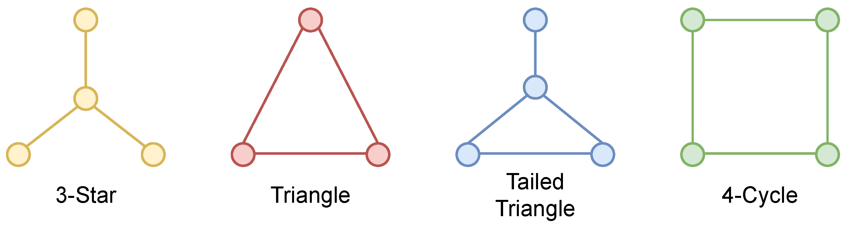
5.6. Graphlet Counting

We evaluate $\mathrm{I}\mathrm{G}\mathrm{E}\mathrm{L}$ on a graphlet counting regression task, training a model to minimize mean squared error (MSE) on the normalized graphlet counts. Counts are normalized by the standard deviation of counts in the training set, as in [26].

In

Table 4. Graphlet counting results. On every cell, we show mean test set MSE error (lower is better), with stat. sig ($p<0.0001$) results highlighted and best results per task underlined. For comparison, we also report strong literature results from two subgraph GNNs: GNN-AK⁺ using a GIN base [21] and SUN [23].

Model	+ $\mathbf{I}\mathbf{G}\mathbf{E}\mathbf{L}$	Star	Triangle	Tailed Tri.	4-Cycle	Custom
Linear	No	$1.60\times {10}^{-1}$	$3.41\times {10}^{-1}$	$2.82\times {10}^{-1}$	$2.03\times {10}^{-1}$	$5.11\times {10}^{-1}$
	Yes	$4.23\times {10}^{-3}$	$4.38\times {10}^{-3}$	$1.85\times {10}^{-2}$	$1.36\times {10}^{-1}$	$5.25\times {10}^{-2}$
MLP	No	$2.66\times {10}^{-6}$	$2.56\times {10}^{-1}$	$1.60\times {10}^{-1}$	$1.18\times {10}^{-1}$	$4.54\times {10}^{-1}$
	Yes	$8.31\times {10}^{-5}$	$5.69\times {10}^{-5}$	$5.57\times {10}^{-5}$	$7.64\times {10}^{-2}$	$2.34\times {10}^{-4}$
GCN	No	$4.72\times {10}^{-4}$	$2.42\times {10}^{-1}$	$1.35\times {10}^{-1}$	$1.11\times {10}^{-1}$	$1.54\times {10}^{-3}$
	Yes	$8.26\times {10}^{-4}$	$1.25\times {10}^{-3}$	$4.15\times {10}^{-3}$	$7.32\times {10}^{-2}$	$1.17\times {10}^{-3}$
GAT	No	$4.15\times {10}^{-4}$	$2.35\times {10}^{-1}$	$1.28\times {10}^{-1}$	$1.11\times {10}^{-1}$	$2.85\times {10}^{-3}$
	Yes	$4.52\times {10}^{-4}$	$6.22\times {10}^{-4}$	$7.77\times {10}^{-4}$	$7.33\times {10}^{-2}$	$6.66\times {10}^{-4}$
GIN	No	$3.17\times {10}^{-4}$	$2.26\times {10}^{-1}$	$1.22\times {10}^{-1}$	$1.11\times {10}^{-1}$	$2.69\times {10}^{-3}$
	Yes	$6.09\times {10}^{-4}$	$1.03\times {10}^{-3}$	$2.72\times {10}^{-3}$	$6.98\times {10}^{-2}$	$2.18\times {10}^{-3}$
Chebnet	No	$5.79\times {10}^{-4}$	$1.71\times {10}^{-1}$	$1.12\times {10}^{-1}$	$8.95\times {10}^{-2}$	$2.06\times {10}^{-3}$
	Yes	$3.81\times {10}^{-3}$	$7.88\times {10}^{-4}$	$2.10\times {10}^{-3}$	$7.90\times {10}^{-2}$	$2.05\times {10}^{-3}$
GNNML3	No	$8.90\times {10}^{-5}$	$2.36\times {10}^{-4}$	$2.91\times {10}^{-4}$	$6.82\times {10}^{-4}$	$9.86\times {10}^{-4}$
	Yes	$9.29\times {10}^{-4}$	$2.19\times {10}^{-4}$	$4.23\times {10}^{-4}$	$6.98\times {10}^{-4}$	$4.17\times {10}^{-4}$
GIN-AK+ [21]	No	$1.6\times {10}^{-2}$	$1.1\times {10}^{-2}$	$1.0\times {10}^{-2}$	$1.1\times {10}^{-2}$	—
SUN [23]	No	$6.0\times {10}^{-3}$	$8.0\times {10}^{-3}$	$8.0\times {10}^{-3}$	$1.1\times {10}^{-2}$	—

, we show the results of introducing $\mathrm{I}\mathrm{G}\mathrm{E}\mathrm{L}$ in five graphlet counting tasks on the RandomGraph data set [54]. We identify 3-stars, triangles, tailed triangles and 4-cycle graphlets, as shown in Figure 6, plus a custom structure with 1-WL expressiveness proposed in [26] to evaluate GNNML3. We highlight statistically significant differences when introducing $\mathrm{I}\mathrm{G}\mathrm{E}\mathrm{L}$ ($p<0.0001$).

Introducing $\mathrm{I}\mathrm{G}\mathrm{E}\mathrm{L}$ improves the ability of 1-WL GNNs to recognize triangles, tailed triangles, and custom 1-WL graphlets from [26]. Stars can be identified by all baselines, and introducing $\mathrm{I}\mathrm{G}\mathrm{E}\mathrm{L}$ only produces statistically significant differences on the linear baseline. Interestingly, $\mathrm{I}\mathrm{G}\mathrm{E}\mathrm{L}$ on the linear model produces results outperforming MP-GNNs without $\mathrm{I}\mathrm{G}\mathrm{E}\mathrm{L}$ for star, triangle, tailed triangle, and custom 1-WL graphlets.

By introducing $\mathrm{I}\mathrm{G}\mathrm{E}\mathrm{L}$ on the MLP baseline, it obtains the best performance (lower MSE) on the triangle, tailed-triangle, and custom 1-WL graphlets, even when compared to GNNML3 and subgraph GNNs—including when $\mathrm{I}\mathrm{G}\mathrm{E}\mathrm{L}$ encodings are input to GNNML3.

Results on linear and MLP baselines are interesting as neither baseline uses message passing, indicating that raw $\mathrm{I}\mathrm{G}\mathrm{E}\mathrm{L}$ encodings may be sufficient to identify certain graph structures in simple linear models. For all graphlets except 4-cycles, introducing $\mathrm{I}\mathrm{G}\mathrm{E}\mathrm{L}$ outperforms or matches GNNML3 performance at lower preprocessing and model training/inference costs—without the need for costly eigen decomposition or message passing, answering Q1 and Q2. $\mathrm{I}\mathrm{G}\mathrm{E}\mathrm{L}$ moderately improves performance counting 4-cycle graphlets, but the results are not competitive when compared to GNNML3.

5.7. Benchmark Results with Subgraph GNNs

Given the favorable performance of $\mathrm{I}\mathrm{G}\mathrm{E}\mathrm{L}$ compared to related subgraph aware methods such as NGNN and ESAN, as shown in Table 2, we also explore introducing $\mathrm{I}\mathrm{G}\mathrm{E}\mathrm{L}$ on a subgraph GNN, namely GNN-AK proposed by [21]. We follow a similar experimental approach as in previous experiments, reproducing the results of GNN-AK using GINs [8] with edge-feature support [55] (GINs are the best performing base model in three out of the four data sets, as reported in [21]) as the base GNN on two real-world benchmark data sets: Zinc-12K (as a graph regression task minimizing mean squared error ↓, where lower is better) and Pattern (as a graph classification task, where higher accuracy ↑ is better) from benchmarking GNNs [50].

Without performing any additional hyper-parameter tuning or architecture search, we evaluate the impact of introducing $\mathrm{I}\mathrm{G}\mathrm{E}\mathrm{L}$ with $\alpha \in \{1,2\}$ on the best performing model configuration and code published by the authors of GNN-AK [21]. Furthermore, we also evaluate the setting in which subgraph information is not used to assess whether $\mathrm{I}\mathrm{G}\mathrm{E}\mathrm{L}$ can provide comparable performance to GNN-AK without changes to the network architecture.

Table 5. Mean and standard deviations of the evaluation metrics on the real-world benchmark data sets in combination with GNN-AK [21], highlighting positive and negative stat. sig, ($p<0.05$) results when $\mathrm{I}\mathrm{G}\mathrm{E}\mathrm{L}$ is added with best per-data set results underlined.

Model	+ $\mathbf{I}\mathbf{G}\mathbf{E}\mathbf{L}$	Zinc-12K (Mean Squared Error, ↓)	Pattern (Accuracy, ↑)
GIN	No	$0.155\pm 0.003$	$85.692\pm 0.042$
	Yes	$0.155\pm 0.005$	$\mathbf{86}.\mathbf{711}\pm \mathbf{0}.\mathbf{009}$
GIN-AK+	No	$0.086\pm 0.002$	$86.877\pm 0.006$
	Yes	$\mathbf{0}.\mathbf{078}\pm \mathbf{0}.\mathbf{003}$	86.737 ± 0.062

↓: lower is better; ↑: higher is better.

summarizes our results.

$\mathrm{I}\mathrm{G}\mathrm{E}\mathrm{L}$ maintains or improves performance in both cases when introduced on a GIN, but only in the case of Pattern we find a statistically significant difference ($p<0.05$). When introducing $\mathrm{I}\mathrm{G}\mathrm{E}\mathrm{L}$ on a GIN-AK model, we find statistically significant improvements on Zinc-12K. Introducing $\mathrm{I}\mathrm{G}\mathrm{E}\mathrm{L}$ on GIN-AK⁺ in Pattern produces unstable losses on the validation set, with model performance showing larger variations across epochs. We believe that this instability might explain the loss in performance and that further hyper-parameter tuning and regularization (e.g., tuning dropout to avoid overfitting on specific $\mathrm{I}\mathrm{G}\mathrm{E}\mathrm{L}$ features) could result in improved model performance.

Finally, we note that despite our constrained setup, introducing $\mathrm{I}\mathrm{G}\mathrm{E}\mathrm{L}$ is also interesting from a runtime and memory standpoint. In particular, introducing $\mathrm{I}\mathrm{G}\mathrm{E}\mathrm{L}$ on a GIN for Pattern yields performance only −0.2% worse than its GNN-AK (86.711 vs. 86.877), while executing 3.87 times faster (62.21 s vs. 240.91 s per iteration) and requiring 20.51 times less memory (26.2 GB vs. 1.3 GB). This is in line with our theoretical analysis in Section 3, as $\mathrm{I}\mathrm{G}\mathrm{E}\mathrm{L}$ can be computed once as a preprocessing step and then introduces a negligible cost on the input size of the first layer, which is amortized in multi-layer GNNs. Together with our results on graph classification, isomorphism detection, and graphlet counting, our experiments show that $\mathrm{I}\mathrm{G}\mathrm{E}\mathrm{L}$ is also an efficient way of introducing subgraph information without architecture modifications in large real-world data sets.

5.8. Link Prediction

We also test $\mathrm{I}\mathrm{G}\mathrm{E}\mathrm{L}$ on a link prediction task, following the approach of [52] to compare with well-known transductive node embedding methods on the Facebook and ArXiv AstroPhysics data sets [56]. We mode the task as follows: for each graph, we generate negative examples (non-existing edges) by sampling random unconnected node pairs. Positive examples (existing edges) are obtained by removing half of the edges, keeping the pruned graph connected after edge removals. Both sets of vertex pairs are chosen to have the same cardinality. Note that keeping the graph connected is not required for $\mathrm{I}\mathrm{G}\mathrm{E}\mathrm{L}$—it is required by transductive methods, which fail to learn meaningful representations on disconnected graph components. We learn self-supervised $\mathrm{I}\mathrm{G}\mathrm{E}\mathrm{L}$ embeddings with a DeepWalk [51] approach (described in Appendix H) and model the link prediction task as a logistic regression problem whose input is the representation of an edge—as the element-wise product of $\mathrm{I}\mathrm{G}\mathrm{E}\mathrm{L}$ embeddings of vertices at each end of an edge without fine-tuning, which is the best edge representation reported by [52].

In

Table 6. Area under the ROC curve (AUROC) link prediction results on Facebook and AP-arXiv. Embeddings learned on $\mathrm{I}\mathrm{G}\mathrm{E}\mathrm{L}$ encodings outperform transductive methods. $\mathrm{I}\mathrm{G}\mathrm{E}\mathrm{L}$ stddevs $<0.005$.

Method	Facebook	arXiv
DeepWalk [51]	0.968	0.934
node2vec [52]	0.968	0.937
$\mathrm{I}\mathrm{G}\mathrm{E}\mathrm{L}$ ($\alpha =2$)	0.976	0.984

, we report AUC results averaged on five independent executions and compared against previous reported baselines. In this case, we perform hyper-parameter search, with results described on Appendix A. We provide additional details on the unsupervised parameters in our code repositories also referenced in Appendix A.

$\mathrm{I}\mathrm{G}\mathrm{E}\mathrm{L}$ with $\alpha =2$ significantly outperforms standard transductive methods on both data sets. This is despite the fact that we compare against methods that are aware of node identities and that several vertices can share the same $\mathrm{I}\mathrm{G}\mathrm{E}\mathrm{L}$ encodings. Furthermore, $\mathrm{I}\mathrm{G}\mathrm{E}\mathrm{L}$ is an inductive method that may be used on unseen nodes and edges, unlike transductive methods DeepWalk or node2vec. We do not explore the inductive setting as it would unfairly favor $\mathrm{I}\mathrm{G}\mathrm{E}\mathrm{L}$ and cannot be directly applied to DeepWalk or Node2vec.

Additionally, $\mathrm{I}\mathrm{G}\mathrm{E}\mathrm{L}$ significantly underperforms when $\alpha =1$. We believe this might be caused by the fact that when $\alpha <2$, it is not possible for the model to assess whether two vertices are neighbors based on their $\mathrm{I}\mathrm{G}\mathrm{E}\mathrm{L}$ representation. Overall, our link prediction results show that $\mathrm{I}\mathrm{G}\mathrm{E}\mathrm{L}$ encodings can be used as a potentially inductive feature generation approach in unattributed networks, without degrading performance when compared to standard vertex embedding methods—answering Q3.

5.9. Vertex Classification

In light of our graph-level results on graphlet counting, we evaluate to which extent a vertex classification task can be solved by leveraging $\mathrm{I}\mathrm{G}\mathrm{E}\mathrm{L}$ structural features without message passing (Q4). We introduce $\mathrm{I}\mathrm{G}\mathrm{E}\mathrm{L}$ in a DNN model and evaluate against several MP-GNN baselines. Our comparison includes supervised baselines proposed by GraphSAGE [32], LCGL [34], and GAT [33] on a multi-label classification task in a protein-to-protein interaction (PPI) [32] data set. The aim is to predict 121 binary labels, given graph data where every vertex has 50 attributes. We tune the parameters of a multi-layer perceptron (MLP) whose input features are either $\mathrm{I}\mathrm{G}\mathrm{E}\mathrm{L}$, vertex attributes, or both through randomized grid search—and we provide a detailed description of the grid-search parameters in Appendix A.

Table 7. Multi-label class. Micro-F1 scores on PPI. $\mathrm{I}\mathrm{G}\mathrm{E}\mathrm{L}$ plus node features as input for an MLP outperforms LGCL and GraphSAGE. $\mathrm{I}\mathrm{G}\mathrm{E}\mathrm{L}$ stddevs $<0.01$.

Method		PPI
Only Features (MLP, ours)		0.558
GraphSAGE-GCN [32]		0.500
GraphSAGE-mean [32]		0.598
GraphSAGE-LSTM [32]		0.612
GraphSAGE-pool [32]		0.600
GraphSAGE (no sampling) [33]		0.768
LGCL [34]		0.772
$\mathrm{I}\mathrm{G}\mathrm{E}\mathrm{L}$ ($\alpha =1$)	Graph Only	0.736
	Graph + Feats	0.850
$\mathrm{I}\mathrm{G}\mathrm{E}\mathrm{L}$ ($\alpha =2$)	Graph Only	0.506
	Graph + Feats	0.741
Const-GAT [33]		0.934
GAT [33]		0.973

shows Micro-F1 scores averaged over five independent runs. Introducing $\mathrm{I}\mathrm{G}\mathrm{E}\mathrm{L}$ alongside vertex attributes in an MLP can outperform standard MP-GNNs like GraphSAGE or LGCL despite not using message passing—and thus only having access to the attributes of a vertex without additional context from its neighbors, answering Q4. Furthermore, even though $\mathrm{I}\mathrm{G}\mathrm{E}\mathrm{L}$ underperforms when compared with GAT, the results reported by [33] use a three-layer GAT model propagating messages through 3-hops, while we observe the best $\mathrm{I}\mathrm{G}\mathrm{E}\mathrm{L}$ performance with $\alpha =1$. We believe that the structural information at 1-hop captured by $\mathrm{I}\mathrm{G}\mathrm{E}\mathrm{L}$ might be sufficient to improve performance on tasks where local information is critical, potentially reducing the hops required by downstream models (e.g., GATs).

6. Discussion and Conclusions

$\mathrm{I}\mathrm{G}\mathrm{E}\mathrm{L}$ is a novel and simple vertex representation algorithm that increases the expressive power of MP-GNNs beyond the 1-WL test. Empirically, we found $\mathrm{I}\mathrm{G}\mathrm{E}\mathrm{L}$ can be used as a vertex/edge feature extractor on graph-, edge-, and node-level settings. On four different graph-level tasks, $\mathrm{I}\mathrm{G}\mathrm{E}\mathrm{L}$ significantly improves the performance of nine graph representation models without requiring architectural modifications—including Linear and MLP baselines, GCNs [57], GATs [33], GINs [8], ChebNets [30], GNNML3 [26], and GNN-AK [21]. We introduce $\mathrm{I}\mathrm{G}\mathrm{E}\mathrm{L}$ without performing hyper-parameter search on an existing baseline, which suggests that $\mathrm{I}\mathrm{G}\mathrm{E}\mathrm{L}$ encodings are informative and can be introduced in a model without costly architecture search.

Although structure-aware message passing [16,20,21,23], substructure counts [19], identity [39], and subgraph pooling [22] may also be combined with existing MP-GNN architectures, $\mathrm{I}\mathrm{G}\mathrm{E}\mathrm{L}$ reaches comparable performance as related models while simply augmenting the set of vertex-level feature without tuning model hyper-parameters. $\mathrm{I}\mathrm{G}\mathrm{E}\mathrm{L}$ consistently improves performance on five data sets for graph classification: one data set for graph regression, two data sets for isomorphism detection, and five different graphlet structures in a graphlet counting task. Furthermore, even though MP-GNNs with learnable subgraph representations are expected to be more expressive since they can freely learn structural characteristics according to optimization objectives, our results show that introducing $\mathrm{I}\mathrm{G}\mathrm{E}\mathrm{L}$ produces comparable results on three different domains and improves the performance of a strong GNN-AK⁺ baseline on Zinc-12K. Additionally, introducing $\mathrm{I}\mathrm{G}\mathrm{E}\mathrm{L}$ on a GIN model in the Pattern data set achieves 99.8% of the performance of a strong GIN-AK⁺ baseline at 3.87 times lower memory costs. The computational efficiency is a key benefit of $\mathrm{I}\mathrm{G}\mathrm{E}\mathrm{L}$ as it only requires a single preprocessing step that extends vertex/edge attributes and can be cached during training and inference.

On link prediction tasks evaluated in two different graph data sets, $\mathrm{I}\mathrm{G}\mathrm{E}\mathrm{L}$-based DeepWalk [51] embeddings outperformed transductive methods based on embedding node identities such as DeepWalk [51] and Node2vec [52]. Finally, $\mathrm{I}\mathrm{G}\mathrm{E}\mathrm{L}$ with $\alpha =1$ outperformed certain MP-GNN architectures like GraphSAGE [32] on a protein–protein interaction node-classification task despite being used as an additional input to a DNN without message passing. More powerful MP-GNNs—namely a three-layer GAT [33]—outperformed the $\mathrm{I}\mathrm{G}\mathrm{E}\mathrm{L}$-enriched DNN model, albeit at potentially higher computational costs due to the increased depth of the model.

A fundamental aspect in our analysis of the expressivity of $\mathrm{I}\mathrm{G}\mathrm{E}\mathrm{L}$ is that the connectivity of nodes is different depending on whether they are analyzed as part of the subgraph (ego network) or within the entire input graph. In particular, edges at the boundary of the ego network are a subset of the edges in the input graph. $\mathrm{I}\mathrm{G}\mathrm{E}\mathrm{L}$ exploits this idea in combination with a simple encoding based on frequencies of degrees and distances. This is a novel idea, which allows us to connect the expressive power of $\mathrm{I}\mathrm{G}\mathrm{E}\mathrm{L}$ with other analyses like the 1-WL test, as well as Weisfeiler–Lehman kernels (see Appendix B), shortest-path neural networks (see Appendix D), and $MATLANG$ (see Appendix E). Furthermore, the ego network formulation allows us to identify an upper-bound on expressivity in strongly regular graphs—matching recent findings on the expressivity of subgraph GNNs.

Although we have presented $\mathrm{I}\mathrm{G}\mathrm{E}\mathrm{L}$ on unattributed graphs, the principle underlying its encoding can be also applied to labelled or attributed graphs. Appendix G outlines possible extensions in this direction. In Appendix G.3, we also connect $\mathrm{I}\mathrm{G}\mathrm{E}\mathrm{L}$ with k-hop GNNs and GNN-AK—drawing a direct link between subgraph GNNs and our proposed encoding.

Overall, our results show that $\mathrm{I}\mathrm{G}\mathrm{E}\mathrm{L}$ can be efficiently used to enrich network representations on a variety of tasks and data sets, which we believe is an attractive baseline in expressivity-related tasks. This opens up interesting future research directions by showing that explicit network encodings like $\mathrm{I}\mathrm{G}\mathrm{E}\mathrm{L}$ can perform competitively compared to more complex learnable representations while being more computationally efficient.

References

1. Bronstein, M.M.; Bruna, J.; Cohen, T.; Veličković, P. Geometric Deep Learning: Grids, Groups, Graphs, Geodesics, and Gauges. arXiv 2021, arXiv:2104.13478. [Google Scholar]
2. Ying, R.; He, R.; Chen, K.; Eksombatchai, P.; Hamilton, W.L.; Leskovec, J. Graph convolutional neural networks for web-scale recommender systems. In Proceedings of the 24th ACM International Conference on Knowledge Discovery & Data Mining, London, UK, 19–23 August 2018; pp. 974–983. [Google Scholar]
3. Duvenaud, D.K.; Maclaurin, D.; Iparraguirre, J.; Bombarell, R.; Hirzel, T.; Aspuru-Guzik, A.; Adams, R.P. Convolutional Networks on Graphs for Learning Molecular Fingerprints. In Proceedings of the Advances in Neural Information Processing Systems, Montreal, Canada, 7–12 December 2015; Volume 28. [Google Scholar]
4. Gilmer, J.; Schoenholz, S.S.; Riley, P.F.; Vinyals, O.; Dahl, G.E. Neural Message Passing for Quantum Chemistry. In Proceedings of the 34th International Conference on Machine Learning, Sydney, Australia, 6–11 August 2017; 2017; Volume 70, pp. 1263–1272. [Google Scholar]
5. Samanta, B.; De, A.; Jana, G.; Gómez, V.; Chattaraj, P.; Ganguly, N.; Gomez-Rodriguez, M. NEVAE: A Deep Generative Model for Molecular Graphs. J. Mach. Learn. Res. 2020, 21, 1–33. [Google Scholar] [CrossRef]
6. Battaglia, P.; Pascanu, R.; Lai, M.; Jimenez Rezende, D.; Kavukcuoglu, K. Interaction Networks for Learning about Objects, Relations and Physics. In Proceedings of the Advances in Neural Information Processing Systems, Barcelona, Spain, 5–10 December 2016; Volume 29. [Google Scholar]
7. Weisfeiler, B.; Leman, A. The Reduction of a Graph to Canonical Form and the Algebra which Appears Therein. Nauchno-Tech. Inf. 1968, 2, 12–16. [Google Scholar]
8. Xu, K.; Hu, W.; Leskovec, J.; Jegelka, S. How Powerful are Graph Neural Networks? In Proceedings of the 7th International Conference on Learning Representations ICLR, New Orleans, LA, USA, 6–9 May 2019. [Google Scholar]
9. Morris, C.; Ritzert, M.; Fey, M.; Hamilton, W.L.; Lenssen, J.E.; Rattan, G.; Grohe, M. Weisfeiler and Leman Go Neural: Higher-Order Graph Neural Networks. In Proceedings of the Thirty-Third AAAI Conference on Artificial Intelligence (AAAI-19), Honolulu, HI, USA, 27 January–1 February 2019; 2019; 33, pp. 4602–4609. [Google Scholar]
10. Grohe, M. Descriptive Complexity, Canonisation, and Definable Graph Structure Theory; Lecture Notes in Logic; Cambridge University Press: Cambridge, UK, 2017. [Google Scholar]
11. Brijder, R.; Geerts, F.; Bussche, J.V.D.; Weerwag, T. On the Expressive Power of Query Languages for Matrices. ACM Trans. Database Syst. 2019, 44, 1–31. [Google Scholar] [CrossRef]
12. Barceló, P.; Kostylev, E.V.; Monet, M.; Pérez, J.; Reutter, J.; Silva, J.P. The Logical Expressiveness of Graph Neural Networks. In Proceedings of the International Conference on Learning Representations, Virtual Conference, 26 April–1 May 2020. [Google Scholar]
13. Geerts, F. On the Expressive Power of Linear Algebra on Graphs. Theory Comput. Syst. 2021, 65, 1–61. [Google Scholar] [CrossRef]
14. Morris, C.; Lipman, Y.; Maron, H.; Rieck, B.; Kriege, N.M.; Grohe, M.; Fey, M.; Borgwardt, K. Weisfeiler and Leman go machine learning: The story so far. arXiv 2021, arXiv:2112.09992. [Google Scholar]
15. You, J.; Ying, R.; Leskovec, J. Position-aware Graph Neural Networks. In Proceedings of the 36th International Conference on Machine Learning, Long Beach, CA, USA, 9–15 June 2019; Volume 97, pp. 7134–7143. [Google Scholar]
16. Nikolentzos, G.; Dasoulas, G.; Vazirgiannis, M. k-hop graph neural networks. Neural Netw. 2020, 130, 195–205. [Google Scholar] [CrossRef] [PubMed]
17. Bodnar, C.; Frasca, F.; Otter, N.; Wang, Y.; Liò, P.; Montufar, G.F.; Bronstein, M. Weisfeiler and Lehman Go Cellular: CW Networks. Adv. Neural Inf. Process. Syst. 2021, 34, 2625–2640. [Google Scholar]
18. Vignac, C.; Loukas, A.; Frossard, P. Building powerful and equivariant graph neural networks with structural message-passing. Adv. Neural Inf. Process. Syst. 2020, 33, 14143–14155. [Google Scholar]
19. Bouritsas, G.; Frasca, F.; Zafeiriou, S.; Bronstein, M.M. Improving Graph Neural Network Expressivity via Subgraph Isomorphism Counting. IEEE Trans. Pattern Anal. Mach. Intell. 2022, 45, 657–668. [Google Scholar] [CrossRef]
20. Zhang, M.; Li, P. Nested graph neural networks. Adv. Neural Inf. Process. Syst. 2021, 34, 15734–15747. [Google Scholar]
21. Zhao, L.; Jin, W.; Akoglu, L.; Shah, N. From Stars to Subgraphs: Uplifting Any GNN with Local Structure Awareness. In Proceedings of the International Conference on Learning Representations, Virtual Conference, 25–29 April 2022. [Google Scholar]
22. Bevilacqua, B.; Frasca, F.; Lim, D.; Srinivasan, B.; Cai, C.; Balamurugan, G.; Bronstein, M.M.; Maron, H. Equivariant Subgraph Aggregation Networks. In Proceedings of the International Conference on Learning Representations, Virtual Conference, 25–29 April 2022. [Google Scholar]
23. Frasca, F.; Bevilacqua, B.; Bronstein, M.M.; Maron, H. Understanding and Extending Subgraph GNNs by Rethinking Their Symmetries. In Proceedings of the Advances in Neural Information Processing Systems, Virtual/New Orleans, LA, USA, 28 November–9 December 2022. [Google Scholar]
24. Michel, G.; Nikolentzos, G.; Lutzeyer, J.; Vazirgiannis, M. Path Neural Networks: Expressive and Accurate Graph Neural Networks. In Proceedings of the 40th International Conference on Machine Learning (ICML), Honolulu, HI, USA, 23–29 July 2023. [Google Scholar]
25. Maron, H.; Ben-Hamu, H.; Serviansky, H.; Lipman, Y. Provably Powerful Graph Networks. In Proceedings of the Advances in Neural Information Processing Systems, Vancouver, Canada, 8–14 December 2019; Volume 32. [Google Scholar]
26. Balcilar, M.; Héroux, P.; Gaüzère, B.; Vasseur, P.; Adam, S.; Honeine, P. Breaking the Limits of Message Passing Graph Neural Networks. In Proceedings of the 38th International Conference on Machine Learning (ICML), Virtual conference, 18–24 July 2021. [Google Scholar]
27. Hu, W.; Fey, M.; Zitnik, M.; Dong, Y.; Ren, H.; Liu, B.; Catasta, M.; Leskovec, J. Open Graph Benchmark: Datasets for Machine Learning on Graphs. In Proceedings of the Advances in Neural Information Processing Systems 33 (NeurIPS 2020), Virtual conference, 6–12 December 2020; Volume 33. [Google Scholar]
28. Morris, C.; Kriege, N.M.; Bause, F.; Kersting, K.; Mutzel, P.; Neumann, M. TUDataset: A collection of benchmark datasets for learning with graphs. In Proceedings of the ICML 2020 Workshop on Graph Representation Learning and Beyond (GRL+ 2020), Virtual conference, 12–18 July 2020. [Google Scholar]
29. You, J.; Ying, Z.; Leskovec, J. Design Space for Graph Neural Networks. Adv. Neural Inf. Process. Syst. 2020, 33, 17009–17021. [Google Scholar]
30. Defferrard, M.; Bresson, X.; Vandergheynst, P. Convolutional Neural Networks on Graphs with Fast Localized Spectral Filtering. In Proceedings of the Advances in Neural Information Processing Systems, Barcelona, Spain, 5–10 December 2016; Volume 29. [Google Scholar]
31. Kipf, T.N.; Welling, M. Semi-Supervised Classification with Graph Convolutional Networks. In Proceedings of the 5th International Conference on Learning Representations ICLR, Toulon, France, 24–26 April 2017. [Google Scholar]
32. Hamilton, W.; Ying, Z.; Leskovec, J. Inductive Representation Learning on Large Graphs. In Proceedings of the Advances in Neural Information Processing Systems 30, Long Beach, USA, 4–9 December 2017. [Google Scholar]
33. Veličković, P.; Cucurull, G.; Casanova, A.; Romero, A.; Liò, P.; Bengio, Y. Graph Attention Networks. In Proceedings of the International Conference on Learning Representations, Vancouver, Canada, 30 April–3 May 2018. [Google Scholar]
34. Gao, H.; Wang, Z.; Ji, S. Large-Scale Learnable Graph Convolutional Networks. In Proceedings of the 24th ACM SIGKDD International Conference on Knowledge Discovery & Data Mining, London, UK, 19–23 August 2018; pp. 1416–1424. [Google Scholar]
35. Babai, L.; Kucera, L. Canonical labelling of graphs in linear average time. In Proceedings of the 20th Annual Symposium on Foundations of Computer Science (sfcs 1979), San Juan, PR, USA, 29–31 October 1979; pp. 39–46. [Google Scholar] [CrossRef]
36. Huang, N.T.; Villar, S. A Short Tutorial on The Weisfeiler–Lehman Test And Its Variants. In Proceedings of the ICASSP 2021-2021 IEEE International Conference on Acoustics, Speech and Signal Processing (ICASSP), Toronto, ON, Canada, 6–11 June 2021; pp. 8533–8537. [Google Scholar]
37. Veličković, P. Message passing all the way up. In Proceedings of the Workshop on Geometrical and Topological Representation Learning, International Conference on Learning Representations, Virtual Conference, 25–29 April 2022. [Google Scholar]
38. Li, P.; Wang, Y.; Wang, H.; Leskovec, J. Distance Encoding: Design Provably More Powerful Neural Networks for Graph Representation Learning. Adv. Neural Inf. Process. Syst. 2020, 33, 4465–4478. [Google Scholar]
39. You, J.; Gomes-Selman, J.M.; Ying, R.; Leskovec, J. Identity-aware graph neural networks. In Proceedings of the Thirty-Fifth AAAI Conference on Artificial Intelligence (AAAI-21), Virtual conference, 2–9 February 2021; 2021; 35, pp. 10737–10745. [Google Scholar]
40. Abboud, R.; Dimitrov, R.; Ceylan, İ.İ. Shortest Path Networks for Graph Property Prediction. In Proceedings of the First Learning on Graphs Conference (LoG), Virtual Conference, 9–12 December 2022. [Google Scholar]
41. Maron, H.; Ben-Hamu, H.; Shamir, N.; Lipman, Y. Invariant and Equivariant Graph Networks. In Proceedings of the International Conference on Learning Representations, New Orleans, LA, USA, 6–9 May 2019. [Google Scholar]
42. Zhang, B.; Luo, S.; Wang, L.; He, D. Rethinking the Expressive Power of GNNs via Graph Biconnectivity. In Proceedings of the International Conference on Learning Representations, Kigali, Rwanda, 1–5 May 2023. [Google Scholar]
43. Papp, P.A.; Wattenhofer, R. A Theoretical Comparison of Graph Neural Network Extensions. In Proceedings of the 39th International Conference on Machine Learning, Baltimore, MD, USA, 17–23 July 2022; 162, pp. 17323–17345. [Google Scholar]
44. Albert, R.; Barabási, A.L. Statistical mechanics of complex networks. Rev. Mod. Phys. 2002, 74, 47–97. [Google Scholar] [CrossRef]
45. Shervashidze, N.; Schweitzer, P.; Jan, E.; Leeuwen, V.; Mehlhorn, K.; Borgwardt, K. Weisfeiler–Lehman Graph Kernels. J. Mach. Learn. Res. 2010, 1, 1–48. [Google Scholar]
46. Alvarez-Gonzalez, N.; Kaltenbrunner, A.; Gómez, V. Beyond 1-WL with Local Ego-Network Encodings. In Proceedings of the First Learning on Graphs Conference (LoG), Virtual Conference, 9–12 December 2022. Non-archival Extended Abstract track. [Google Scholar]
47. Van Dam, E.R.; Haemers, W.H. Which Graphs Are Determined by Their Spectrum? Linear Algebra Its Appl. 2003, 373, 241–272. [Google Scholar] [CrossRef]
48. Brouwer, A.E. and Van Maldeghem, Hendrik. Strongly Regular Graphs; Cambridge University Press: Cambridge, UK, 2022; Volume 182, p. 462. [Google Scholar]
49. Arvind, V.; Fuhlbrück, F.; Köbler, J.; Verbitsky, O. On Weisfeiler-Leman invariance: Subgraph counts and related graph properties. J. Comput. Syst. Sci. 2020, 113, 42–59. [Google Scholar] [CrossRef]
50. Dwivedi, V.P.; Joshi, C.K.; Laurent, T.; Bengio, Y.; Bresson, X. Benchmarking Graph Neural Networks. arXiv 2020, arXiv:2003.00982. [Google Scholar]
51. Perozzi, B.; Al-Rfou, R.; Skiena, S. DeepWalk: Online Learning of Social Representations. In Proceedings of the 20th ACM SIGKDD International Conference on Knowledge Discovery and Data Mining, New York, NY, USA, 24–27 August 2014; pp. 701–710. [Google Scholar]
52. Grover, A.; Leskovec, J. Node2Vec: Scalable Feature Learning for Networks. In Proceedings of the 22nd ACM SIGKDD International Conference on Knowledge Discovery and Data Mining, San Francisco, CA, USA, 13–17 August 2016; pp. 855–864. [Google Scholar]
53. Abboud, R.; Ceylan, I.I.; Grohe, M.; Lukasiewicz, T. The Surprising Power of Graph Neural Networks with Random Node Initialization. In Proceedings of the International Joint Conferences on Artificial Intelligence Organization, Virtual Conference, 19–26 August 2021; pp. 2112–2118. [Google Scholar]
54. Chen, Z.; Chen, L.; Villar, S.; Bruna, J. Can Graph Neural Networks Count Substructures? Adv. Neural Inf. Process. Syst. 2020, 33, 10383–10395. [Google Scholar]
55. Hu, W.; Liu, B.; Gomes, J.; Zitnik, M.; Liang, P.; Pande, V.; Leskovec, J. Strategies for Pre-training Graph Neural Networks. In Proceedings of the International Conference on Learning Representations, Virtual Conference, 26 April–1 May 2020. [Google Scholar]
56. Leskovec, J.; Krevl, A. SNAP Datasets: Stanford Large Network Dataset Collection. 2014. Available online: https://snap.stanford.edu/data/index.html (accessed on 16 September 2023).
57. Niepert, M.; Ahmed, M.; Kutzkov, K. Learning Convolutional Neural Networks for Graphs. In Proceedings of the 33rd International Conference on Machine Learning, New York, NY, USA, 19–24 June 2016; Volume 48, pp. 2014–2023. [Google Scholar]
58. Shervashidze, N.; Borgwardt, K. Fast subtree kernels on graphs. In Proceedings of the Advances in Neural Information Processing Systems, Vancouver, Canada, 7–12 December 2009; Volume 22. [Google Scholar]
59. Rieck, B.; Bock, C.; Borgwardt, K. A Persistent Weisfeiler–Lehman Procedure for Graph Classification. In Proceedings of the 36th International Conference on Machine Learning, Long Beach, CA, USA, 9–15 June 2019; 2019; Volume 97, pp. 5448–5458. [Google Scholar]
60. Togninalli, M.; Ghisu, E.; Llinares-López, F.; Rieck, B.; Borgwardt, K. Wasserstein Weisfeiler–Lehman Graph Kernels. Adv. Neural Inf. Process. Syst. 2019, 32, 6436–6446. [Google Scholar]
61. Kriege, N.M.; Morris, C.; Rey, A.; Sohler, C. A Property Testing Framework for the Theoretical Expressivity of Graph Kernels. In Proceedings of the Twenty-Seventh International Joint Conference on Artificial Intelligence (IJCAI-18), Stockholm, Sweden, 13–19 July 2018; 2018; Volume 7, pp. 2348–2354. [Google Scholar]
62. Mikolov, T.; Sutskever, I.; Chen, K.; Corrado, G.; Dean, J. Distributed Representations of Words and Phrases and Their Compositionality. In Proceedings of the 26th International Conference on Neural Information Processing Systems, Lake Tahoe, USA, 5–10 December 2013; Volume 2, pp. 3111–3119. [Google Scholar]
Figure 1. I G E L encoding of the green vertex. Dashed region denotes E v α ( α = 2 ) . The green vertex is at distance 0, blue vertices at 1, and red vertices at 2. Labels show degrees in E v α . The frequency of distance degree ( l ˜ , d ˜ ) tuples forming I G E L vec α ( v ) is: { ( 0 , 2 ) : 1 , ( 1 , 2 ) : 1 , ( 1 , 4 ) : 1 , ( 2 , 3 ) : 2 , ( 2 , 4 ) : 1 } .
Make 05 00063 g001
Figure 2. Decalin (top) and Bicyclopentyl (bottom). 1-WL (Algorithm 1) produces equivalent colorings in both graphs; hence, they are 1-WL equivalent. The colorings match between central nodes (purple), their immediate neighbors (blue), and peripheral nodes farthest from the center (green).
Make 05 00063 g002
Figure 3. I G E L encodings ( α { 1 , 2 } ) for Decalin and Bicyclopentyl computed for purple vertices (v). Dotted sections are not encoded. Colors denote different ( l ˜ , d ˜ ) tuples. I G E L ( α = 2 ) distinguishes the graphs since Decalin nodes at distance 2 from v have degree 1 (green) while their Bicyclopentyl counterparts have degrees 1 (green) and 2 (red).
Make 05 00063 g003
Figure 4. I G E L encodings for two co-spectral 4-regular graphs from [47]. I G E L distinguishes 4 kinds of structures within the graphs (associated with every node as a, b, c, and d). The two graphs can be distinguished since the encoded structures and their frequencies do not match.
Make 05 00063 g004
Figure 5. 3-WL equivalent 4 × 4 Rook ((a), red) and Shrikhande ((b), blue) graphs are indistinguishable by I G E L as they are non-isomorphic SRGs with parameters SRG ( 16 , 6 , 2 , 2 ) .
Make 05 00063 g005
Figure 6. Graphlet types in the counting task.
Make 05 00063 g006