Author Contributions
Conceptualization, C.P.N., S.V. and B.S.; Data curation, C.P.N. and S.V.; Formal analysis, C.P.N.; Funding acquisition, B.S.; Investigation, C.P.N.; Methodology, C.P.N. and S.V.; Project administration, S.V. and B.S.; Resources, B.S.; Software, C.P.N. and S.V.; Supervision, S.V. and B.S.; Validation, C.P.N.; Visualization, C.P.N.; Writing—original draft, C.P.N.; Writing—review and editing, C.P.N., S.V. and B.S. All authors have read and agreed to the published version of the manuscript.
Figure 1.
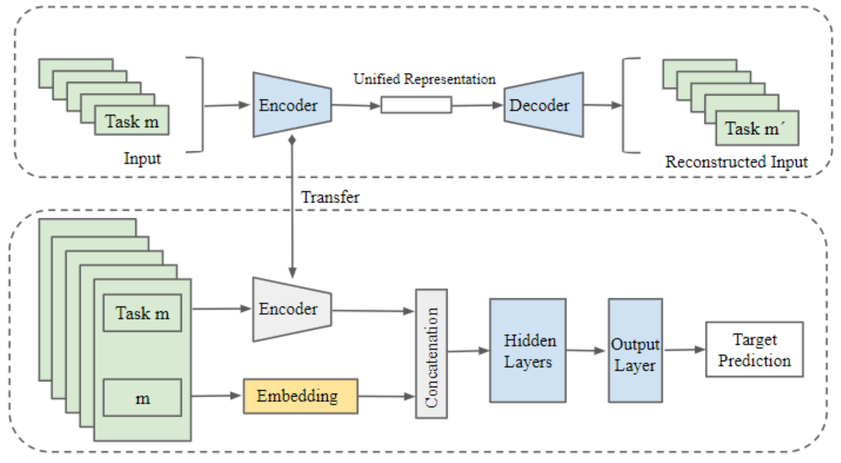
The figure represents the UAE-TENN (Unified Autoencoder-Task-Embedding Neural Network) architecture. In this architecture, the task features are indicated in green, trainable neural network layers in blue, task-specific embedding in orange, and non-trainable layers in grey. The upper portion demonstrates Unified Autoencoder training using multi-task input data. The encoder thus learned is utilized in the lower portion, which represents training a neural network with encoded input and task embedding.
Figure 1.
The figure represents the UAE-TENN (Unified Autoencoder-Task-Embedding Neural Network) architecture. In this architecture, the task features are indicated in green, trainable neural network layers in blue, task-specific embedding in orange, and non-trainable layers in grey. The upper portion demonstrates Unified Autoencoder training using multi-task input data. The encoder thus learned is utilized in the lower portion, which represents training a neural network with encoded input and task embedding.
Figure 2.
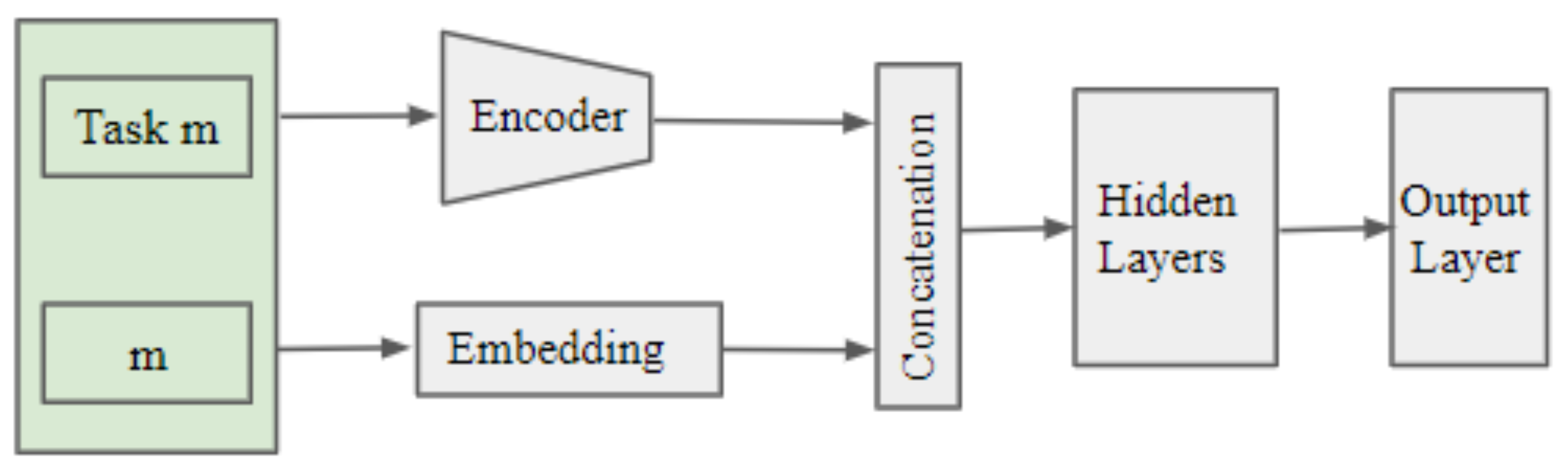
The task-specific inference procedure using UAE-TENN architecture. This picture showcases the inference procedure for task m.
Figure 2.
The task-specific inference procedure using UAE-TENN architecture. This picture showcases the inference procedure for task m.
Figure 3.
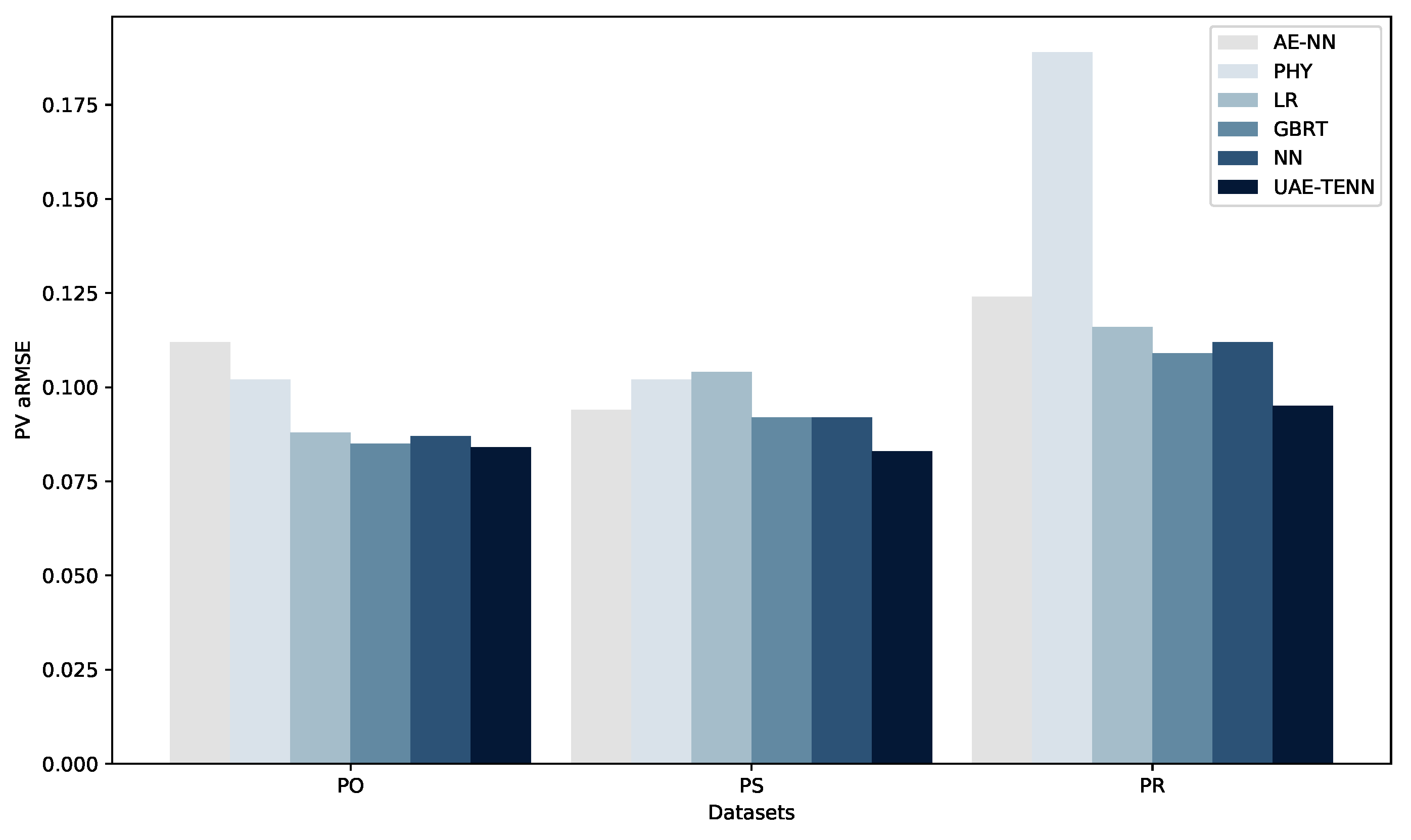
Comparison of aRMSE values among STL methods across three PV datasets PO, PS and PR.
Figure 3.
Comparison of aRMSE values among STL methods across three PV datasets PO, PS and PR.
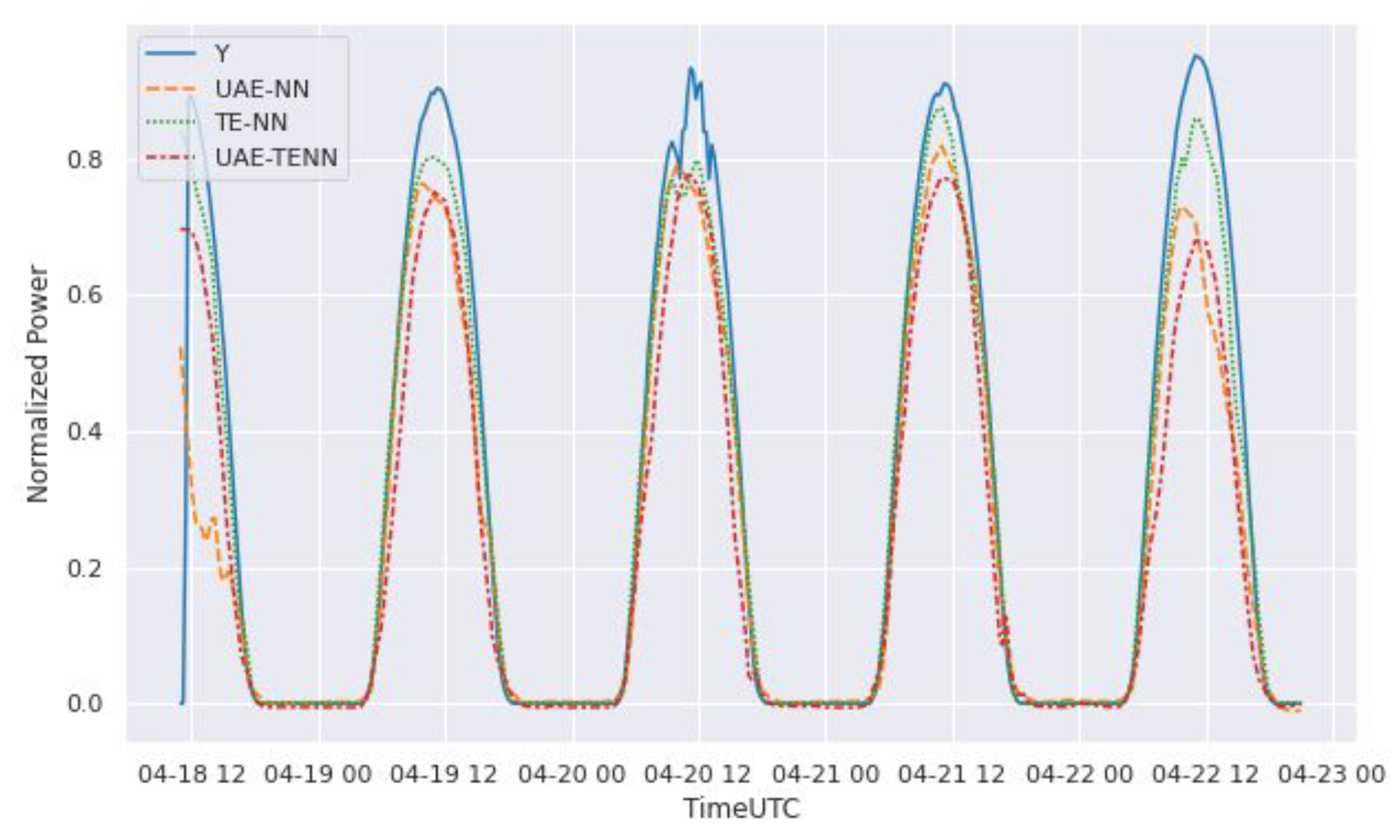
Figure 4.
Exemplary power forecast comparison of MTL methods for a PV park from the real-world dataset. The X-axis represents the time and Y axis represents the normalized power generation. The solid blue line (Y) represents the actual power generated by the park and the other three dotted lines represent the predicted values by different MTL models.
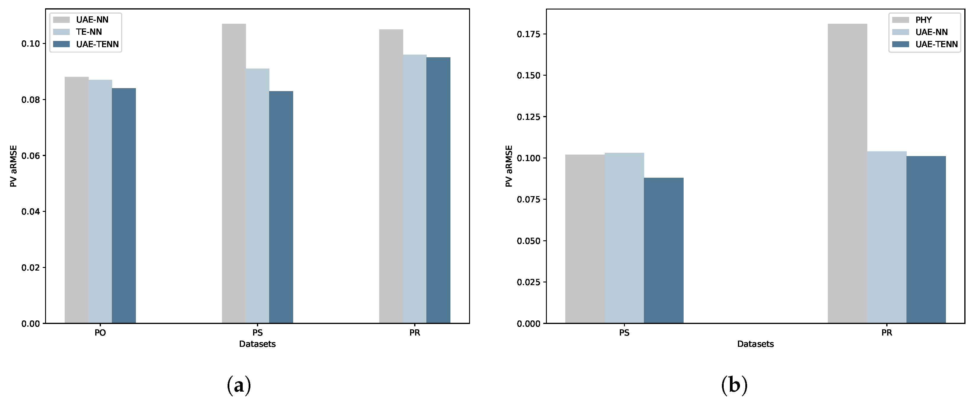
Figure 5.
MTL and ZSL comparison plots. (a) Comparison of aRMSE values among MTL methods across three PV datasets PO, PS, and PR. (b) Comparison of aRMSE values among ZSL methods across three PV datasets PO, PS, and PR.
Figure 5.
MTL and ZSL comparison plots. (a) Comparison of aRMSE values among MTL methods across three PV datasets PO, PS, and PR. (b) Comparison of aRMSE values among ZSL methods across three PV datasets PO, PS, and PR.
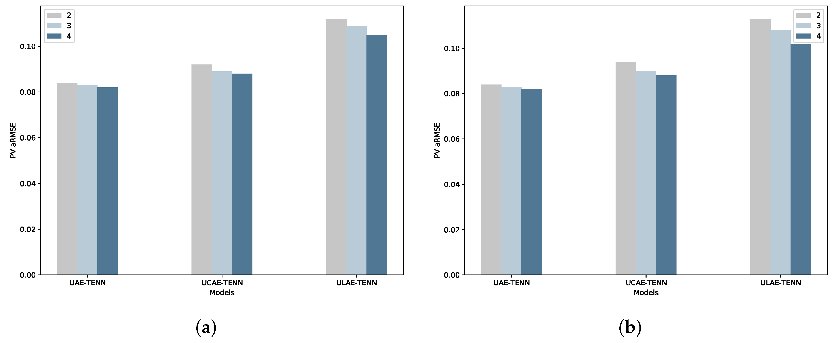
Figure 6.
MTL and ZSL comparison plots. (a) Comparison of aRMSE values for MTL with varying task embedding dimensions across three unified autoencoder models for the PS dataset. (b) Comparison of aRMSE values for ZSL with varying task embedding dimensions across three unified autoencoder models for the PS dataset.
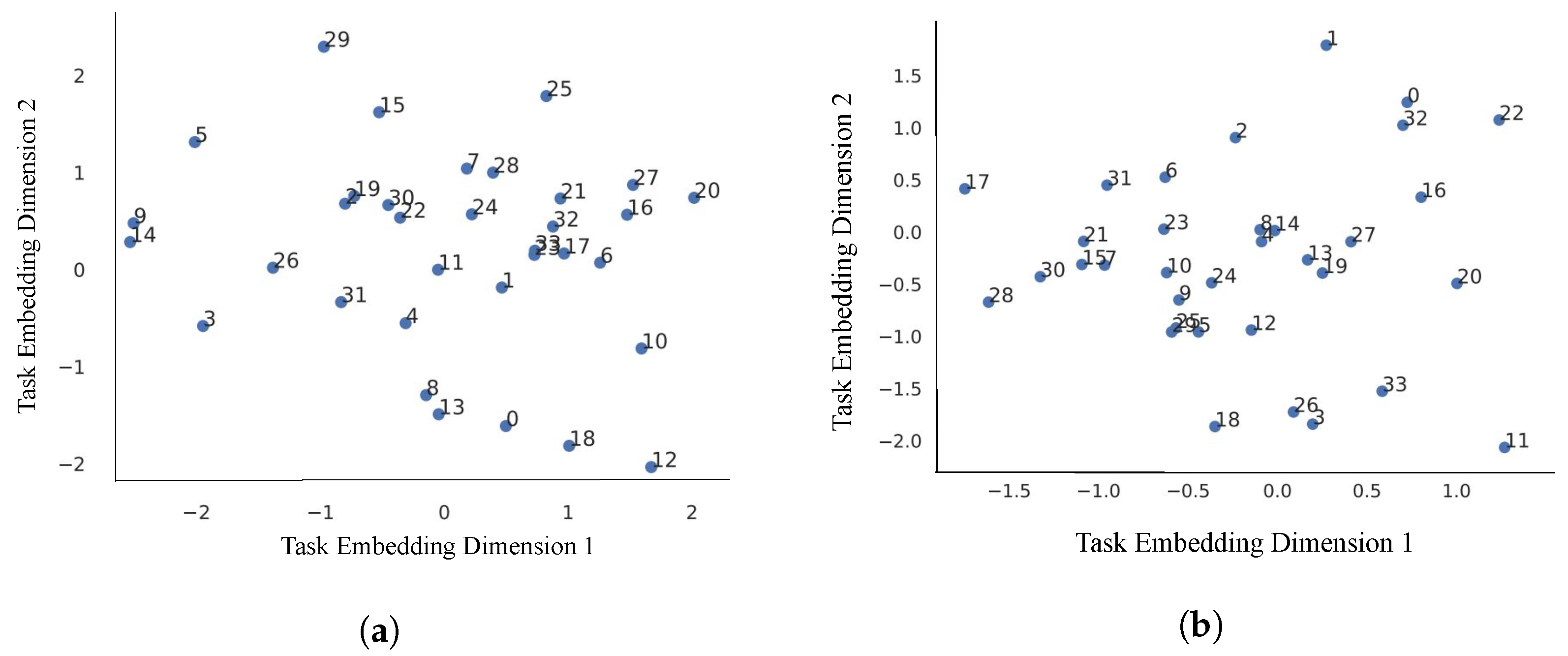
Figure 7.
Task embeddings visualization plots. (a) Visualization of two-dimensional task embeddings learned from UCAE-TENN architecture for PR dataset. (b) Visualization of two-dimensional task embeddings learned from ULAE-TENN architecture for PR dataset.
Figure 7.
Task embeddings visualization plots. (a) Visualization of two-dimensional task embeddings learned from UCAE-TENN architecture for PR dataset. (b) Visualization of two-dimensional task embeddings learned from ULAE-TENN architecture for PR dataset.
Table 1.
Datasets overview with source parks and target zero-shot parks information.
Table 1.
Datasets overview with source parks and target zero-shot parks information.
| Dataset | # Features | # Total Parks | Source Data | | Target Zero-Shot Data | |
|---|
| # Parks | # Mean Train
Samples | # Mean Test
Samples | | # Parks | # Mean Train
Samples | # Mean Test
Samples | |
|---|
| Pv Open (PO) | 51 | 21 | 17 | 4553 | 1518 | | 4 | 4371 | 1457 | |
| Wind Open (WO) | 7 | 45 | 36 | 11,462 | 3821 | | 9 | 9287 | 3096 | |
| Pv Synthetic (PS) | 14 | 118 | 94 | 8405 | 4234 | | 24 | 8158 | 4225 | |
| Wind Synthetic (WS) | 24 | 118 | 94 | 8467 | 4223 | | 24 | 8466 | 4288 | |
| Pv Real (PR) | 19 | 42 | 34 | 59,166 | 19,722 | | 8 | 53,892 | 17,964 | |
| Wind Real (WR) | 27 | 185 | 148 | 46,405 | 15,468 | | 37 | 36,289 | 12,096 | |
Table 2.
Evaluation results of STL methods with UAE-TENN for three different PV power datasets. The asterisk (*) symbol indicates significantly different aRMSE values of reference than baseline (AE-NN) tested through a one-sided Wilcoxon signed-rank test with = 0.05. The bold values in a column indicates best performance. Additionally, it’s important to note that both open-source datasets, PO and WO, contain NA values for the PHY model, as there are no available PHY model results.
| Model Type | PV aRMSE | | PV Skill | | PV Std | |
|---|
| PO | PS | PR | | PO | PS | PR | | PO | PS | PR | |
|---|
| AE-NN | 0.112 | 0.094 * | 0.124 | | 0.000 | 0.000 | 0.000 | | 0.022 | 0.015 | 0.019 | |
| PHY | NA | 0.102 | 0.189 | | NA | −0.084 | −0.587 | | NA | 0.016 | 0.199 | |
| LR | 0.088 * | 0.104 | 0.116 * | | 0.218 | −0.096 | 0.064 | | 0.022 | 0.019 | 0.019 | |
| GBRT | 0.085 * | 0.092 | 0.109 * | | 0.239 | 0.023 | 0.120 | | 0.021 | 0.014 | 0.019 | |
| NN | 0.087 * | 0.092 * | 0.112 * | | 0.221 | 0.021 | 0.094 | | 0.023 | 0.013 | 0.020 | |
| UAE-TENN | 0.084 * | 0.083 * | 0.095 * | | 0.245 | 0.118 | 0.222 | | 0.020 | 0.013 | 0.011 | |
| Mean UAE-TENN | 0.087 | | 0.195 | | 0.014 | |
Table 3.
Evaluation results of STL methods with UAE-TENN for three different wind power datasets. The asterisk (*) symbol indicates significantly different aRMSE values of reference than baseline (AE-NN) tested through a one-sided Wilcoxon signed-rank test with = 0.05. The bold values in a column indicate the best performance.
| Model Type | Wind aRMSE | | Wind Skill | | Wind Std | |
|---|
| WO | WS | WR | | WO | WS | WR | | WO | WS | WR | |
|---|
| AE-NN | 0.132 | 0.141 | 6.124 | | 0.000 | 0.000 | 0.000 | | 0.040 | 0.054 | 65.143 | |
| PHY | NA | 0.255 | 0.201 | | NA | −1.259 | −0.181 | | NA | 0.095 | 0.069 | |
| LR | 0.123 | 0.156 | 1.515 * | | 0.042 | −0.355 | −0.007 | | 0.031 | 0.047 | 10.234 | |
| GBRT | 0.112 * | 0.144 | 0.158 * | | 0.133 | −0.235 | 0.088 | | 0.032 | 0.041 | 0.043 | |
| NN | 0.110 * | 0.137 * | 2.598 * | | 0.145 | −0.041 | −0.037 | | 0.031 | 0.039 | 18.377 | |
| UAE-TENN | 0.117 * | 0.142 | 0.142 * | | 0.096 | −0.078 | 0.153 | | 0.032 | 0.041 | 0.029 | |
| Mean UAE-TENN | 0.133 | | 0.057 | | 0.034 | |
Table 4.
Evaluation results of MTL methods with UAE-TENN for three PV datasets with baseline UAE-NN as a baseline model. The asterisk (*) symbol indicates significantly different aRMSE values of reference than baseline (AE-NN) tested through a one-sided Wilcoxon signed-rank test with = 0.05. The bold values in a column indicate the best performance.
| Model Type | PV aRMSE | | PV Skill | | PV Std | |
|---|
| PO | PS | PR | | PO | PS | PR | | PO | PS | PR | |
|---|
| UAE-NN | 0.088 | 0.107 | 0.105 | | 0.000 | 0.000 | 0.000 | | 0.024 | 0.021 | 0.020 | |
| TENN | 0.087 | 0.091 * | 0.096 * | | −0.006 | 0.136 | 0.080 | | 0.020 | 0.015 | 0.014 | |
| UAE-TENN | 0.084 * | 0.083 * | 0.095 * | | 0.029 | 0.209 | 0.087 | | 0.020 | 0.013 | 0.011 | |
| Mean UAE-TENN | 0.087 | | 0.108 | | 0.014 | |
Table 5.
Evaluation results of MTL methods with UAE-TENN for three wind datasets with baseline UAE-NN as a baseline model. The asterisk (*) symbol indicates significantly different aRMSE values of reference than baseline (AE-NN) tested through a one-sided Wilcoxon signed-rank test with = 0.05. The bold values in a column indicate the best performance.
| Model Type | Wind aRMSE | | Wind Skill | | Wind Std | |
|---|
| WO | WS | WR | | WO | WS | WR | | WO | WS | WR | |
|---|
| UAE-NN | 0.156 | 0.199 | 0.175 | | 0.000 | 0.000 | 0.000 | | 0.036 | 0.083 | 0.045 | |
| TENN | 0.115 * | 0.146 * | 0.148 * | | 0.267 | 0.218 | 0.140 | | 0.031 | 0.040 | 0.030 | |
| UAE-TENN | 0.117 * | 0.142 * | 0.142 * | | 0.253 | 0.240 | 0.173 | | 0.032 | 0.041 | 0.029 | |
| Mean UAE-TENN | 0.133 | | 0.222 | | 0.034 | |
Table 6.
Evaluation results of ZSL methods with UAE-TENN for four datasets with PHY as a baseline model. The asterisk (*) symbol indicates significantly different aRMSE values of reference than baseline (AE-NN) tested through a one-sided Wilcoxon signed-rank test with = 0.05. The bold values in a column indicate the best performance.
| Model Type | PV aRMSE | | Wind aRMSE | | PV Skill | | Wind Skill | | PV Std | | Wind Std | |
|---|
| PS | PR | | WS | WR | | PS | PR | | WS | WR | | PS | PR | | WS | WR | |
|---|
| PHY | 0.102 | 0.181 | | 0.212 | 0.187 | | 0.000 | 0.000 | | 0.000 | 0.000 | | 0.018 | 0.156 | | 0.047 | 0.061 | |
| UAE-NN | 0.103 | 0.104 | | 0.213 * | 0.172 * | | −0.009 | 0.226 | | −0.076 | 0.049 | | 0.026 | 0.017 | | 0.138 | 0.039 | |
| UAE-TENN | 0.088 * | 0.101 * | | 0.220 | 0.180 | | 0.145 | 0.247 | | −0.110 | −0.020 | | 0.024 | 0.016 | | 0.159 | 0.042 | |
| Mean UAE-TENN | 0.094 | | 0.200 | | 0.196 | | −0.065 | | 0.020 | | 0.100 | |
Table 7.
Comparison of regular, convolutional, and LSTM autoencoders in the proposed architecture for three different datasets in STL inference evaluation. The asterisk (*) symbol indicates significantly different aRMSE values of reference than baseline (AE-NN) tested through a one-sided Wilcoxon signed-rank test with = 0.05. The bold values in a column indicate the best performance.
| Model Type | PV aRMSE | | PV Skill | | PV Std | |
|---|
| PO | PS | PR | | PO | PS | PR | | PO | PS | PR | |
|---|
| UAE-TENN | 0.085 * | 0.084 * | 0.111 * | | 0.236 | 0.108 | 0.100 | | 0.021 | 0.013 | 0.018 | |
| UCAE-TENN | 0.088 * | 0.091 * | 0.111 * | | 0.213 | 0.032 | 0.097 | | 0.019 | 0.014 | 0.111 | |
| ULAE-TENN | 0.108 | 0.114 | 0.138 | | 0.029 | −0.216 | −0.117 | | 0.023 | 0.022 | 0.138 | |
Table 8.
Comparison of results for ZSL methods on two datasets with PHY as a baseline model. The asterisk (*) symbol indicates significantly different aRMSE values of reference than baseline (AE-NN) tested through a one-sided Wilcoxon signed-rank test with = 0.05. The bold values in a column indicate the best performance.
| Model Type | PV aRMSE | | PV skill | | PV Std | |
|---|
| PS | PR | | PS | PR | | PS | PR | |
|---|
| UAE-TENN | 0.085 | 0.108 * | | 0.159 | 0.194 | | 0.015 | 0.037 | |
| UCAE-TENN | 0.091 | 0.106 * | | 0.101 | 0.210 | | 0.019 | 0.042 | |
| ULAE-TENN | 0.110 | 0.135 | | −0.087 | 0.018 | | 0.022 | 0.035 | |
Table 9.
Impact of the number of embedding dimensions on aRMSE for three model architectures across two datasets PS and PR in STL inference evaluation.
Table 9.
Impact of the number of embedding dimensions on aRMSE for three model architectures across two datasets PS and PR in STL inference evaluation.
| Model Type | UAE-TENN | | UCAE-TENN | | ULAE-TENN | |
|---|
| PS | PR | | PS | PR | | PS | PR | |
|---|
| 2 | 0.084 | 0.111 | | 0.092 | 0.113 | | 0.112 | 0.137 | |
| 3 | 0.083 | 0.110 | | 0.089 | 0.111 | | 0.109 | 0.137 | |
| 4 | 0.082 | 0.110 | | 0.088 | 0.111 | | 0.105 | 0.136 | |
Table 10.
Impact of the number of embedding dimensions on aRMSE for three model architectures across two datasets PS and PR in ZSL scenario evaluation.
Table 10.
Impact of the number of embedding dimensions on aRMSE for three model architectures across two datasets PS and PR in ZSL scenario evaluation.
| Model Type | UAE-TENN | | UCAE-TENN | | ULAE-TENN | |
|---|
| PS | PR | | PS | PR | | PS | PR | |
|---|
| 2 | 0.084 | 0.108 | | 0.094 | 0.108 | | 0.113 | 0.127 | |
| 3 | 0.083 | 0.107 | | 0.090 | 0.107 | | 0.108 | 0.126 | |
| 4 | 0.082 | 0.106 | | 0.088 | 0.106 | | 0.102 | 0.126 | |


