A Unified Framework for Free Vibration Analysis of Variable-Angle Tow Composite Shells with Spatially Varying Curvature

Abstract

The combination of variable-angle tow composites with shell geometries presents significant potential in various engineering and technical applications, particularly with regard to structural performance. Nevertheless, the numerical modeling of these structures can be challenging, as the larger number of unknowns significantly increases computational effort. The Carrera’s unified formulation has demonstrated promising results in the analysis of plates and shells reinforced with curvilinear fibers, offering an effective balance between numerical accuracy and the number of variables. This paper extends the unified formulation to more complex variable-angle tow shell structures characterized by variable curvature radii within their physical domain. The governing equations of the dynamic problem are derived using a displacement-based variational method, and the results are validated through comparisons with reference solutions from Abaqus 3D models. The First-Order Shear Deformation Theory (FSDT) is presented for a broader comparison of the proposed models. The maximum percentage error in terms of frequency shift observed for the FSDT model is $3.44\%$, whereas the corresponding error for the most refined model is only $0.19\%$. Across all examined cases, the computed fundamental frequencies and mode shapes closely match the reference results, demonstrating the reliability and effectiveness of the proposed method.

1. Introduction

Shell structures are widely recognized across various engineering and technological applications due to their excellent stiffness-to-weight ratio. These structures are particularly advantageous in meeting strict design constraints, as they offer high mechanical performance while maintaining a relatively low overall weight. For instance, shell structures are often integrated into complex engineering systems, including energy-absorbing components [1]. Over the past century, significant advancements in shell theory have been made, particularly with the extension of these theories to the Finite Element Method (FEM), enhancing their applicability in computational analyses. General knowledge on shell theory is comprehensively documented in numerous texts, with fundamental contributions from authors such as Reddy [2], Kraus [3], Leissa [4], Bathe [5] and Washizu [6]. Despite the extensive analysis of shell structures, most studies have focused predominantly on composite materials, with relatively few addressing the integration of shell geometries with VAT laminations. Advances in modern manufacturing technologies have made it possible to revolutionize the traditional concept of composites by aligning fibers along curvilinear paths to create VAT materials. This approach allows for greater optimization of composite properties, significantly enhancing design flexibility and performance potential. However, the FEM analysis of VAT shells presents new challenges due to the introduction of curvatures and continuously varying fiber angles. These characteristics generate new variables into the model, leading to increased complexity in computational analyses. VAT materials and shell structures have been studied through various methods, which are briefly presented in the following text. Analytical and semi-analytical solutions for the dynamic analysis of shell structures where proposed by various authors [7,8,9,10]. Although these solutions demonstrate good accuracy in predicting eigenfrequencies, their applicability is often restricted to specific boundary conditions and particular analysis cases. For example, Yang et al. [11] tried to overcome this problem by using modified Fourier series to represent displacement functions within the Rayleigh–Ritz method for the dynamic analysis of sandwich shells. Subsequently, after the introduction of FEM, various shell models where developed to extend the possibility to solve the dynamic problem for structures with different boundary conditions and geometries. In this context, it is possible to consider the works developed by Aksu [12], Chakravorty, Sinha and Bandyopadhyay [13] and Chaubey, Kumar, and Chakrabarti [14]. Several studies have addressed the formulation of quadrilateral shell elements, yet these models often suffer from overly stiff behavior. This issue primarily stems from the simultaneous presence of shear and membrane locking effects, which are typical in such formulations [15]. To overcome these drawbacks, Bathe and Dvorkin [16] introduced the mixed interpolation of tensorial components approach, developing robust four- and eight-node shell elements.

The Carrera Unified Formulation (CUF) has been extensively applied to the analysis of composite structures, offering the ability to extract three-dimensional (3D) stress fields from two-dimensional (2D) models. This approach provides highly accurate results by optimizing the balance between numerical precision and computational efficiency, making it applicable to a wide range of structural analyses. The core principle of CUF lies in its flexibility to predefine functions that describe the behavior of primary variables through the thickness, allowing for the representation of both low- and high-order theories within a unified framework. This adaptability enhances its effectiveness in capturing complex structural behaviors (see [17]). Various early works developed cuf through semi-analytical approaches, investigating the static, modal and thermo-mechanical response of plate and beam structures [18,19,20]. For instance, Giunta et al. [21] used CUF to investigate the thermo-mechanical behavior of beam structures through a strong form solution employing Wendland’s radial basis functions. CUF was subsequently expanded to FEM analyses of beams, plates and shells, as shown by De Pietro et al. [22], Pagani, Valvano and Carrera [23] and Cinefra and Carrera [24]. Cinefra, Chinosi, and Della Croce [25] evaluated the effectiveness of the CUF-based nine-node shell element by examining classical benchmark problems. The versatility of CUF also stems from its ability to be adapted to variational formulations beyond the classical principle of virtual displacements. Several studies have extended CUF within the framework of Reissner’s Mixed Variational Theorem (RMVT), enabling the consideration of both displacements and transverse stresses as primary variables in the analysis. For example, Cinefra, Carrera and Kumar [26] used RMVT to develop CUF shell elements for the static analysis of laminated composite plates and shells. Most studies that analyze composite shells using the Carrera Unified Formulation (CUF) focus on structures with constant curvature radii. However, an exception is found in the works of Carrera and Zozulya [27,28,29], who employed CUF for the static analysis of shells of revolution, utilizing numerical solutions obtained with Mathematica software. The unified formulation has demonstrated high accuracy in multi-field analyses, effectively capturing the coupling between mechanical, thermal, electrical, and magnetic field variables. Owing to the versatility of CUF in representing the behavior of primary variables through the structure thickness, several studies have extended its application beyond purely mechanical problems. For instance, Carrera and Nali [30] employed CUF to model multi-field effects in multilayered plate elements. More recently, Monge et al. [31] conducted a static analysis of magneto-electro-elastic shells with variable curvature radii by combining CUF with the differential quadrature method. Additional multi-field extensions of CUF to shell elements have also been presented in various works [32,33].

The concept of Variable Angle Tow (VAT) composites has been developed over recent decades and can be effectively applied to modern structures to enhance their mechanical properties. Hyer and Charette [34] demonstrated that curvilinear fibers can improve the mechanical performance of plates with internal cutouts, using an element-wise representation of fiber patterns. More recent works, such as the paper by Gürdal, Tatting, and Wu [35], have shown the capability to simulate a continuous variation in fiber angles across the plate domain. Tornabene, Fantuzzi, and Bacciocchi [36] employed the CUF framework to perform static analyses of shells reinforced with curvilinear fibers, where the GDQ method was adopted to handle the numerical solution. Sánchez-Majano et al. [37] analyzed the static response of VAT cylindrical shells using CUF-based models. Furthermore, Sciascia et al. [38] extended the application of CUF to VAT shells, investigating their buckling, free vibration, and prestressed vibration behaviors. Daghighi et al. [39] studied the design of ellipsoidal shells of revolution using VAT composites to achieve a bend-free state, where the structure resists internal pressure without bending or curvature changes. The dynamic instability analysis of prestressed variable stiffness composite shell structures was performed by Sciascia, Oliveri and Weaver [40] through the Ritz method. The works from Montemurro and Catapano [41,42] showed the efficiency of the multi-scale two-level approach for the optimization of VAT composites. The postbuckling response of VAT shells was optimized by Liguori et al. [43] through an isogeometric framework employing non-uniform rational basis spline interpolation functions. The investigation of the linear buckling behavior of VAT shell structures was conducted by Miao et al. [44] through isogeometric analysis.

Although extensive research has been devoted to shell structures, studies applying CUF to the free vibration analysis of VAT shells of revolution are still relatively scarce. Furthermore, to the best of the authors’ knowledge, CUF has not yet been employed to investigate the dynamic response of VAT shells with variable curvature radii. Indeed, the previously cited works using CUF for shell geometries are based on the hypothesis that the curvatures and the first quadratic form coefficients of the structure mid-surface remain constant, which allows to simplify the geometrical relations, and consequently the stiffness matrix fundamental nuclei. Commercial FEM software, such as Abaqus, typically offer a wide range of two-dimensional shell elements that inherently account for the aforementioned geometric complexities. Nevertheless, these elements generally lack flexibility in defining the order of through-thickness polynomial expansions, which are often limited to low-order approximations. In addition, the implementation of curvilinear fiber paths in such software is subject to significant constraints, preventing the representation of continuously varying fiber orientations and instead resulting in an element-wise discretisation of the fiber pattern. This study aims to fill the existing research gap by employing CUF for the modal analysis of shells characterized by variable curvature, implementing a formulation where continuously varying fiber distributions can be represented. The principal innovation introduced lies in the geometric formulation of the analyzed structures, specifically within the displacement–strain relationships, which incorporate the derivatives of curvature radii and geometric coefficients directly into the shell kinematics. The remainder of this paper is organized as follows. Section 2 outlines the fundamentals of the CUF framework and its implementation for VAT shells through a displacement-based modeling approach. Section 3 investigates the free vibration behavior of several representative geometries, including toroidal, ellipsoidal, and hyperboloid shells. The computed eigenfrequencies are validated against reference solutions obtained using three-dimensional finite element models in Abaqus. Finally, Section 4 summarizes the main findings and provides concluding remarks.

2. Problem Description

The region occupied by a shell structure can be defined as the Cartesian closed-point subset

$$V=\Omega \times \left[-h/2,h/2\right],$$

(1)

of the 3D space ${\mathbb{R}}^3$, where h represents the thickness. $\Omega$ is the mid-surface of the shell which can be defined in the ${\mathbb{R}}^2$ space as follows:

$$\Omega =\left\{(\alpha ,\beta ):{\displaystyle \frac{\alpha }{l_{\alpha }}},{\displaystyle \frac{\beta }{l_{\beta }}}\in [0,1]\right\}.$$

(2)

The curvilinear coordinates, denoted by $\alpha$ and $\beta$, lie on the mid-surface of the shell, while the z-axis is oriented along the shell thickness. The parameters $l_{\alpha }$ and $l_{\beta }$ denote the characteristic dimensions along the $\alpha$- and $\beta$-directions, respectively. The position vector $\mathit{r}$ defines a point on the undeformed mid-surface of the shell and is expressed in the global Cartesian coordinate system $OXYZ$, as illustrated in Figure 1:

$$\mathit{r}=\mathit{r}\left(\alpha ,\beta \right)$$

(3)

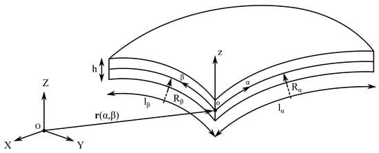
Figure 1. Shell geometry and reference system.

The infinitesimal variation of the vector $\mathit{r}$ can be defined as:

$$d\mathit{r}=\mathit{r}{,}_{\alpha }d\alpha +\mathit{r}{,}_{\beta }d\beta$$

(4)

where the comma denotes differentiation with respect to the curvilinear coordinate axes. The magnitudes of the corresponding derivative vectors are given by:

$$\begin{array}{c}|\mathit{r}{,}_{\alpha }|=A,\hfill \\ |\mathit{r}{,}_{\beta }|=B.\hfill \end{array}$$

(5)

The following unit vectors can be introduced:

$$\begin{array}{c}{\mathit{i}}_{\alpha }=\mathit{r}{,}_{\alpha }/A,\hfill \\ {\mathit{i}}_{\beta }=\mathit{r}{,}_{\beta }/B,\hfill \\ {\mathit{i}}_n={\mathit{i}}_{\alpha }\times {\mathit{i}}_{\beta }/sin\left(\chi \right).\hfill \end{array}$$

(6)

Here, ${\mathit{i}}_{\alpha }$ and ${\mathit{i}}_{\beta }$ denote the unit tangent vectors along the $\alpha$ and $\beta$ directions, respectively, while ${\mathit{i}}_n$ represents the unit vector through the thickness, obtained as the cross product of ${\mathit{i}}_{\alpha }$ and ${\mathit{i}}_{\beta }$. The parameter $\chi$ defines the angle between the mid-surface coordinate axes $\alpha$ and $\beta$. The right-hand side of the following equation corresponds to the first quadratic form of the mid-surface:

$$d\mathit{r}d\mathit{r}=A^{2}d{\alpha }^2+2ABcos\left(\chi \right)d\alpha d\beta +B^{2}d{\beta }^2.$$

(7)

The second quadratic form is associated with determining the curvature of an arbitrary curve on the surface. For conciseness, only the final expression for the normal curvature of the surface is provided:

$${\displaystyle \frac{1}{R}}=-{\displaystyle \frac{Ld{\alpha }^2+2Md\alpha d\beta +Nd{\beta }^2}{A^{2}d{\alpha }^2+2ABcos\left(\chi \right)d\alpha d\beta +B^{2}d{\beta }^2}},$$

(8)

where the numerator of the right-hand side of the equation is the second quadratic form of the surface. The following terms can be introduced:

$$\begin{array}{c}L=\mathit{r}{,}_{\alpha \alpha }{\mathit{i}}_n,\hfill \\ M=\mathit{r}{,}_{\alpha \beta }{\mathit{i}}_n,\hfill \\ N=\mathit{r}{,}_{\beta \beta }{\mathit{i}}_n.\hfill \end{array}$$

(9)

The curvatures of $\alpha$ and $\beta$ lines can be obtained by considering $\beta$ and $\alpha$ as constants, respectively:

$$\begin{array}{c}1/R_{\alpha }=-L/A^2,\hfill \\ 1/R_{\beta }=-N/B^2.\hfill \end{array}$$

(10)

Assuming that $\alpha$ and $\beta$ are the principal curvature lines of the surface simplifies the shell equations. The necessary and sufficient conditions for $\alpha$ and $\beta$ to be principal curvature lines are as follows:

$$\begin{array}{c}cos\left(\chi \right)=0,\hfill \\ M=0.\hfill \end{array}$$

(11)

The location of a generic point within the shell domain can be written as:

$$\mathit{R}\left(\alpha ,\beta ,z\right)=\mathit{r}\left(\alpha ,\beta \right)+z{\mathit{i}}_n\left(\alpha ,\beta \right),$$

(12)

where z is the thickness coordinate. The square of the modulus of an infinitesimal change of the R vector can be written as follows:

$$d\mathit{R}d\mathit{R}=H_{\alpha }^{2}d{\alpha }^2+H_{\beta }^{2}d{\beta }^2+H_z^{2}d{z}^2,$$

(13)

where

$$\begin{array}{c}{H}_{\alpha }=A\left(1+z/R_{\alpha }\right),\hfill \\ H_{\beta }=B\left(1+z/R_{\beta }\right),\hfill \\ H_z=1.\hfill \end{array}$$

(14)

Subsequently, the infinitesimal surface and volume of the fundamental shell element can be written:

$$\begin{array}{c}d\Omega =H_{\alpha }{H}_{\beta }d\alpha d\beta ,\hfill \\ dV=H_{\alpha }{H}_{\beta }{H}_{z}d\alpha d\beta dz.\hfill \end{array}$$

(15)

A schematic representation of curvilinear coordinates and principal directions is reported in Figure 2.

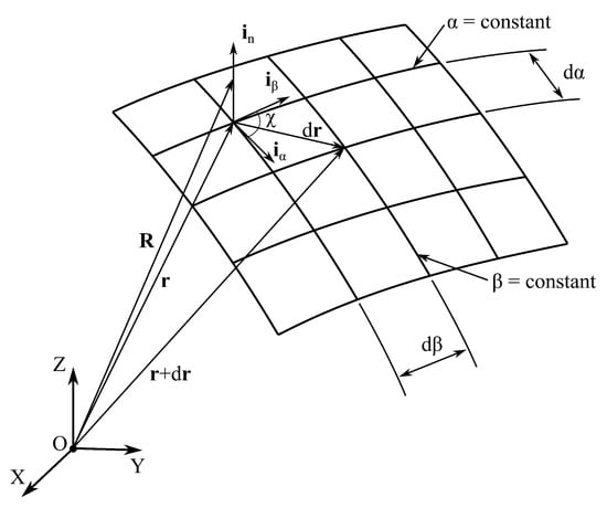
Figure 2. Middle surface coordinates.

Since this work considers shells of revolution with variable radii of curvature, a general formulation of the governing equations is adopted, enabling their use for shells in which $R_{\alpha }$ and $R_{\beta }$ change over the mid-surface. The displacement field is expressed as:

$$\mathit{u}=\left\{\begin{array}{c}{u}_{\alpha }\\ u_{\beta }\\ u_z\end{array}\right\}.$$

(16)

The mid-surface and through-the-thickness components of the strain vector can be expressed as:

$${\mathit{ϵ}}_p=\left\{\begin{array}{c}{ϵ}_{\alpha \alpha }\\ {ϵ}_{\beta \beta }\\ {ϵ}_{\alpha \beta }\end{array}\right\},{\mathit{ϵ}}_n=\left\{\begin{array}{c}{ϵ}_{\alpha z}\\ {ϵ}_{\beta z}\\ {ϵ}_{zz}\end{array}\right\}.$$

(17)

A linear strains-displacements relation is considered, according to the hypothesis of small displacements:

$$\begin{array}{c}{\mathit{ϵ}}_p=\left({\mathit{D}}_p+{\mathit{A}}_p\right)\mathit{u},\hfill \\ {\mathit{ϵ}}_n=\left({\mathit{D}}_{n\Omega }+{\mathit{A}}_n+{\mathit{D}}_{nz}\right)\mathit{u},\hfill \end{array}$$

(18)

where ${\mathit{D}}_p,{\mathit{D}}_{n\Omega }$ and ${\mathit{D}}_{nz}$ are differential operators:

$${\mathit{D}}_p=\left[\begin{array}{ccc}{\displaystyle \frac{\partial \alpha }{H_{\alpha }}}& 0& 0\\ 0& {\displaystyle \frac{\partial \beta }{H_{\beta }}}& 0\\ {\displaystyle \frac{\partial \beta }{H_{\beta }}}& {\displaystyle \frac{\partial \alpha }{H_{\alpha }}}& 0\end{array}\right],{\mathit{D}}_{n\Omega }=\left[\begin{array}{ccc}0& 0& {\displaystyle \frac{\partial \alpha }{H_{\alpha }}}\\ 0& 0& {\displaystyle \frac{\partial \beta }{H_{\beta }}}\\ 0& 0& 0\end{array}\right],{\mathit{D}}_{nz}=\left[\begin{array}{ccc}\partial z& 0& 0\\ 0& \partial z& 0\\ 0& 0& \partial z\end{array}\right].$$

(19)

The matrices ${\mathit{A}}_p$ and ${\mathit{A}}_n$ are written as follows:

$${\mathit{A}}_p=\left[\begin{array}{ccc}0& {\displaystyle \frac{A{,}_{\beta }}{B{H}_{\alpha }}}& {\displaystyle \frac{A}{H_{\alpha }{R}_{\alpha }}}\\ {\displaystyle \frac{B{,}_{\alpha }}{A{H}_{\beta }}}& 0& {\displaystyle \frac{B}{H_{\beta }{R}_{\beta }}}\\ -{\displaystyle \frac{H_{\alpha {,}_{\beta }}}{H_{\alpha }{H}_{\beta }}}& -{\displaystyle \frac{H_{\beta {,}_{\alpha }}}{H_{\alpha }{H}_{\beta }}}& 0\end{array}\right],{\mathit{A}}_{n\Omega }=\left[\begin{array}{ccc}-{\displaystyle \frac{A}{H_{\alpha }{R}_{\alpha }}}& 0& 0\\ 0& -{\displaystyle \frac{B}{H_{\beta }{R}_{\beta }}}& 0\\ 0& 0& 0\end{array}\right].$$

(20)

The stress components on the mid-surface and in the transverse direction are expressed as follows:

$${\mathit{\sigma }}_p=\left\{\begin{array}{c}{\sigma }_{\alpha \alpha }\\ {\sigma }_{\beta \beta }\\ {\sigma }_{\alpha \beta }\end{array}\right\},{\mathit{\sigma }}_n=\left\{\begin{array}{c}{\sigma }_{\alpha z}\\ {\sigma }_{\beta z}\\ {\sigma }_{zz}\end{array}\right\}.$$

(21)

Hooke’s law reads:

$$\begin{array}{c}{\mathit{\sigma }}_p={\tilde{\mathit{C}}}_{pp}{\mathit{ϵ}}_p+{\tilde{\mathit{C}}}_{pn}{\mathit{ϵ}}_n,\hfill \\ {\mathit{\sigma }}_n={\tilde{\mathit{C}}}_{np}{\mathit{ϵ}}_p+{\tilde{\mathit{C}}}_{nn}{\mathit{ϵ}}_n,\hfill \end{array}$$

(22)

where the terms ${\tilde{\mathit{C}}}_{pp},{\tilde{\mathit{C}}}_{pn},{\tilde{\mathit{C}}}_{np}$ and ${\tilde{\mathit{C}}}_{nn}$ are the components of the material stiffness matrix. Table 1 summarizes the main hypotheses that are considered within this work.

Table 1. Summary of theoretical assumptions.

	Hypothesis
Displacement-strain relations (Equation (18))	A linear relation between displacement and strain fields is assumed. Hence, strains vary linearly with displacements.
Strain-stress relations (Equation (22))	A linear elastic material behavior is considered, meaning stresses vary linearly with strains according to Hooke’s law.
Curvilinear coordinate system	The coordinates $\alpha$ and $\beta$ correspond to principal lines of curvature, which means that $\alpha$-constant and $\beta$-constant curvatures are orthogonal and they form a conjugate system (Equation (11)).

2.1. Variable Angle-Tow Composite Shells

VAT composites are characterized by fibers whose orientation $\theta$ can vary locally along the mid-surface directions. This work considers a linear law to describe fibers angle, which can be expressed as follows:

$$\theta \left(\alpha \right)=\Phi +T_0+{\displaystyle \frac{T_1-T_0}{d}}\left|{\alpha }^{\prime }\right|.$$

(23)

The geometrical meaning of ${\alpha }^{\prime }$, $\Phi$, $T_0$, d and $T_1$ is graphically represented in Figure 3. Knowing $\theta$ at each point of the shell middle-surface, the material stiffness matrix $\mathit{C}$ can be rotated to obtain $\tilde{C}$. For the sake of brevity, the details related to the rotation are not discussed here and can be found in the literature works [2]. The following notation is used to describe fibers path along the middle surface: $\Phi <T_0,T_1>$.

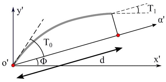
Figure 3. Example of in-plane fibers path.

Although a linear law for the fiber angle distribution is adopted here for demonstration purposes, the developed code is capable of handling any arbitrary variation law. This is possible because the integrals over the shell mid-surface are evaluated using Gauss quadrature, which only requires knowledge of the material stiffness coefficients at the integration points. When higher-order functions are used for describing $\theta$, an increased number of integration points is necessary to accurately capture the variation of fiber angles within each element domain. In previous studies, more advanced distributions, such as parabolic variation laws, have also been successfully implemented [45].

2.2. Carrera’s Unified Formulation

In the unified formulation, an axiomatic expansion technique is adopted to represent the primary unknowns along the z coordinate [17]. Considering the adaptation of CUF to a finite element framework, the representation of the displacement vector $\mathit{u}\left(\alpha ,\beta ,z\right)$, for a 2D element corresponds to:

$$\mathit{u}\left(\alpha ,\beta ,z\right)=F_{\tau }\left(z\right)N_i\left(\alpha ,\beta \right){\mathit{q}}_{\tau i},\tau =0,1,\dots ,N,i=1,\dots ,N_n,$$

(24)

where $N_i$ denotes the shape functions employed to interpolate the unknown field variables over the shell mid-surface, and $N_n$ corresponds to the total number of nodes used for the discretisation of the domain. This work uses classical Lagrange shape functions, which can be found in milestone research works about FEM (see, e.g., Zienkiewicz, Taylor and Zhu [46]). The recurrence of an index within an expression denotes summation across its full range. The index $\tau$ varies from zero to the maximum expansion order N, while index i identifies the nodes of the shell domain discretisation, and $N_n$ is the total number of nodes. The capability of CUF to specify a priori both N and $F_{\tau }$, enables the systematic derivation of multiple structural theories within a single unified framework.

The choice of the polynomials $F_{\tau }$, allows to obtain either Equivalent Single Layer (ESL) or Layer-Wise (LW) models. In the ESL approach, the number of primary variables remains constant regardless of the number of physical layers in the laminate, making it efficient for modeling thin structures while maintaining low computational cost. However, the accuracy of ESL models decreases for thick or highly anisotropic laminates, where interlaminar effects become significant. To enhance model precision, the LW approach can be employed, where the kinematic behavior of each layer is treated independently. Nevertheless, LW models come with increased computational costs due to independent approximations for each layer. Further insights on ESL and LW models, including common polynomial choices for through-the-thickness approximations, have been discussed in previous works [47].

2.3. Locking Correction

To mitigate locking phenomena, the Mixed Interpolation of Tensorial Components (MITC) technique is adopted. In the local coordinate system $(\xi ,\eta )$, the MITC formulation defines shell elements by interpolating specific strain components at a priori selected tying points within the element domain. For the shell elements with nine nodes (QUAD9) employed in this work, three distinct tying point configurations are employed, as illustrated in Figure 4.

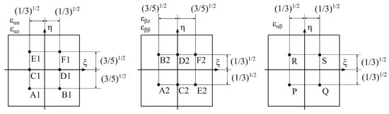
Figure 4. Tying point locations for the nine-node MITC shell element.

Lagrange functions are considered, each specified with respect to the corresponding tying points pattern. These functions are presented through a vector notation as:

$${\mathit{N}}_{m1}={\left\{\begin{array}{c}{N}_{A1}\\ N_{B1}\\ N_{C1}\\ N_{D1}\\ N_{E1}\\ N_{F1}\end{array}\right\}}^T,{\mathit{N}}_{m2}={\left\{\begin{array}{c}{N}_{A2}\\ N_{B2}\\ N_{C2}\\ N_{D2}\\ N_{E2}\\ N_{F2}\end{array}\right\}}^T,{\mathit{N}}_{m3}={\left\{\begin{array}{c}{N}_P\\ N_Q\\ N_R\\ N_S\end{array}\right\}}^T$$

(25)

The in-plane and transverse strain components are interpolated as follows:

$${\mathit{ϵ}}_p=\left[\begin{array}{c}{ϵ}_{\xi \xi }\hfill \\ {ϵ}_{\eta \eta }\hfill \\ {ϵ}_{\xi \eta }\hfill \end{array}\right]=\left[\begin{array}{ccc}{\mathit{N}}_{m1}& 0& 0\\ 0& {\mathit{N}}_{m2}& 0\\ 0& 0& {\mathit{N}}_{m3}\end{array}\right]\left[\begin{array}{c}{\mathit{ϵ}}_{\xi {\xi }_{m1}}\hfill \\ {\mathit{ϵ}}_{\eta {\eta }_{m2}}\hfill \\ {\mathit{ϵ}}_{\xi {\eta }_{m3}}\hfill \end{array}\right]=\mathit{N}\mathbf{1}\left[\begin{array}{c}{\mathit{ϵ}}_{\xi {\xi }_{m1}}\hfill \\ {\mathit{ϵ}}_{\eta {\eta }_{m2}}\hfill \\ {\mathit{ϵ}}_{\xi {\eta }_{m3}}\hfill \end{array}\right],$$

(26)

$${\mathit{ϵ}}_n=\left[\begin{array}{c}{ϵ}_{\xi z}\hfill \\ {ϵ}_{\eta z}\hfill \\ {ϵ}_{zz}\hfill \end{array}\right]=\left[\begin{array}{ccc}{\mathit{N}}_{m1}& 0& 0\\ 0& {\mathit{N}}_{m2}& 0\\ 0& 0& 1\end{array}\right]\left[\begin{array}{c}{\mathit{ϵ}}_{\xi z_{m1}}\hfill \\ {\mathit{ϵ}}_{\eta z_{m2}}\hfill \\ {ϵ}_{zz}\hfill \end{array}\right]=\mathit{N}\mathbf{2}\left[\begin{array}{c}{\mathit{ϵ}}_{\xi z_{m1}}\hfill \\ {\mathit{ϵ}}_{\eta z_{m2}}\hfill \\ {ϵ}_{zz}\hfill \end{array}\right],$$

(27)

in which the subscripts $m1$, $m2$ and $m3$ indicate the functions values at the corresponding tying points sets (A1, B1, C1, D1, E1, F1), (A2, B2, C2, D2, E2, F2) and (P, Q, R, S), respectively.

2.4. Governing Equations

In the PVD case, the primary unknown field is the displacements field. The expression for the virtual internal work is given by:

$$\delta L_{int}={\int }_{\Omega }{\int }_h\left(\delta {\mathit{ϵ}}_{pG}^T{\mathit{\sigma }}_{pH}+\delta {\mathit{ϵ}}_{nG}^T{\mathit{\sigma }}_{nH}\right)dzd\Omega ,$$

(28)

where $\delta$ stands for a virtual variation, the subscript G refers to the components obtained from geometrical relations in Equation (18), subscript H refers to the components obtained from Hooke’s law in Equation (22) and subscript T refers to the transpose of a vector/matrix. Regarding the virtual work of the inertial forces, the following equation can be written:

$$\delta L_{ine}={\int }_{\Omega }{\int }_h\delta {\mathit{u}}^T\rho \ddot{\mathit{u}}dzd\Omega ,$$

(29)

where $\rho$ is the shell material density, and $\ddot{\mathit{u}}$ represents the acceleration vector. For free vibration analyses, the eigenvalue problem can be formulated by imposing:

$$\delta L_{int}+\delta L_{ine}=0.$$

(30)

Through the substitution of Equations (18), (22), (24), (28) and (29) into Equation (30), the governing equations of the PVD method can be obtained:

$$\begin{array}{cc}\hfill {\int }_{\Omega }& \delta {\mathit{q}}_{\tau i}^T[{\left(\mathit{N}{\mathbf{1}}_m{\mathit{D}}_p\right)}^T\left(N_i\mathit{I}\right){\tilde{\mathit{Z}}}_{pp}^{\tau s}\left(\mathit{N}{\mathbf{1}}_o{\mathit{D}}_p\right)\left(N_j\mathit{I}\right)+{\left(\mathit{N}{\mathbf{1}}_m{\mathit{D}}_p\right)}^T\left(N_i\mathit{I}\right){\tilde{\mathit{Z}}}_{pp}^{\tau s}\left(\mathit{N}{\mathbf{1}}_o{\mathit{A}}_p\right)\left(N_j\mathit{I}\right)+\hfill \\ \hfill +& {\left(\mathit{N}{\mathbf{1}}_m{\mathit{D}}_p\right)}^T\left(N_i\mathit{I}\right){\tilde{\mathit{Z}}}_{pn}^{\tau s}\left(\mathit{N}{\mathbf{2}}_o{\mathit{D}}_{n\Omega }\right)\left(N_j\mathit{I}\right)+{\left(\mathit{N}{\mathbf{1}}_m{\mathit{D}}_p\right)}^T\left(N_i\mathit{I}\right){\tilde{\mathit{Z}}}_{pn}^{\tau s}\left(\mathit{N}{\mathbf{2}}_o{\mathit{A}}_n\right)\left(N_j\mathit{I}\right)+\hfill \\ \hfill +& {\left(\mathit{N}{\mathbf{1}}_m{\mathit{D}}_p\right)}^T\left(N_i\mathit{I}\right){\tilde{\mathit{Z}}}_{pn}^{\tau s{,}_z}\mathit{N}{\mathbf{2}}_o\left(N_j\mathit{I}\right)+{\left(\mathit{N}{\mathbf{1}}_m{\mathit{A}}_p\right)}^T\left(N_i\mathit{I}\right){\tilde{\mathit{Z}}}_{pp}^{\tau s}\left(\mathit{N}{\mathbf{1}}_o{\mathit{D}}_p\right)\left(N_j\mathit{I}\right)+\hfill \\ \hfill +& {\left(\mathit{N}{\mathbf{1}}_m{\mathit{A}}_p\right)}^T\left(N_i\mathit{I}\right){\tilde{\mathit{Z}}}_{pp}^{\tau s}\left(\mathit{N}{\mathbf{1}}_o{\mathit{A}}_p\right)\left(N_j\mathit{I}\right)+{\left(\mathit{N}{\mathbf{1}}_m{\mathit{A}}_p\right)}^T\left(N_i\mathit{I}\right){\tilde{\mathit{Z}}}_{pn}^{\tau s}\left(\mathit{N}{\mathbf{2}}_o{\mathit{D}}_{n\Omega }\right)\left(N_j\mathit{I}\right)+\hfill \\ \hfill +& {\left(\mathit{N}{\mathbf{1}}_m{\mathit{A}}_p\right)}^T\left(N_i\mathit{I}\right){\tilde{\mathit{Z}}}_{pn}^{\tau s}\left(\mathit{N}{\mathbf{2}}_o{\mathit{A}}_n\right)\left(N_j\mathit{I}\right)+{\left(\mathit{N}{\mathbf{1}}_m{\mathit{A}}_p\right)}^T\left(N_i\mathit{I}\right){\tilde{\mathit{Z}}}_{pn}^{\tau s{,}_z}\mathit{N}{\mathbf{2}}_o\left(N_j\mathit{I}\right)+\hfill \\ \hfill +& {\left(\mathit{N}{\mathbf{2}}_m{\mathit{D}}_{n\Omega }\right)}^T\left(N_i\mathit{I}\right){\tilde{\mathit{Z}}}_{np}^{\tau s}\left(\mathit{N}{\mathbf{1}}_o{\mathit{D}}_p\right)\left(N_j\mathit{I}\right)+{\left(\mathit{N}{\mathbf{2}}_m{\mathit{D}}_{n\Omega }\right)}^T\left(N_i\mathit{I}\right){\tilde{\mathit{Z}}}_{np}^{\tau s}\left(\mathit{N}{\mathbf{1}}_o{\mathit{A}}_p\right)\left(N_j\mathit{I}\right)+\hfill \\ \hfill +& {\left(\mathit{N}{\mathbf{2}}_m{\mathit{D}}_{n\Omega }\right)}^T\left(N_i\mathit{I}\right){\tilde{\mathit{Z}}}_{nn}^{\tau s}\left(\mathit{N}{\mathbf{2}}_o{\mathit{D}}_{n\Omega }\right)\left(N_j\mathit{I}\right)+{\left(\mathit{N}{\mathbf{2}}_m{\mathit{D}}_{n\Omega }\right)}^T\left(N_i\mathit{I}\right){\tilde{\mathit{Z}}}_{nn}^{\tau s}\left(\mathit{N}{\mathbf{2}}_o{\mathit{A}}_n\right)\left(N_j\mathit{I}\right)+\hfill \\ \hfill +& {\left(\mathit{N}{\mathbf{2}}_m{\mathit{D}}_{n\Omega }\right)}^T\left(N_i\mathit{I}\right){\tilde{\mathit{Z}}}_{nn}^{\tau s{,}_z}\mathit{N}{\mathbf{2}}_o\left(N_j\mathit{I}\right)+{\left(\mathit{N}{\mathbf{2}}_m{\mathit{A}}_n\right)}^T\left(N_i\mathit{I}\right){\tilde{\mathit{Z}}}_{np}^{\tau s}\left(\mathit{N}{\mathbf{1}}_o{\mathit{D}}_p\right)\left(N_j\mathit{I}\right)+\hfill \\ \hfill +& {\left(\mathit{N}{\mathbf{2}}_m{\mathit{A}}_n\right)}^T\left(N_i\mathit{I}\right){\tilde{\mathit{Z}}}_{np}^{\tau s}\left(\mathit{N}{\mathbf{1}}_o{\mathit{A}}_p\right)\left(N_j\mathit{I}\right)+{\left(\mathit{N}{\mathbf{2}}_m{\mathit{A}}_n\right)}^T\left(N_i\mathit{I}\right){\tilde{\mathit{Z}}}_{nn}^{\tau s}\left(\mathit{N}{\mathbf{2}}_o{\mathit{D}}_{n\Omega }\right)\left(N_j\mathit{I}\right)+\hfill \\ \hfill +& {\left(\mathit{N}{\mathbf{2}}_m{\mathit{A}}_n\right)}^T\left(N_i\mathit{I}\right){\tilde{\mathit{Z}}}_{nn}^{\tau s}\left(\mathit{N}{\mathbf{2}}_o{\mathit{A}}_n\right)\left(N_j\mathit{I}\right)+{\left(\mathit{N}{\mathbf{2}}_m{\mathit{A}}_n\right)}^T\left(N_i\mathit{I}\right){\tilde{\mathit{Z}}}_{nn}^{\tau s{,}_z}\mathit{N}{\mathbf{2}}_o\left(N_j\mathit{I}\right)+\hfill \\ \hfill +& \mathit{N}{\mathbf{2}}_m\left(N_i\mathit{I}\right){\tilde{\mathit{Z}}}_{np}^{\tau {,}_{z}s}\left(\mathit{N}{\mathbf{1}}_o{\mathit{D}}_p\right)\left(N_j\mathit{I}\right)+\mathit{N}{\mathbf{2}}_m\left(N_i\mathit{I}\right){\tilde{\mathit{Z}}}_{np}^{\tau {,}_{z}s}\left(\mathit{N}{\mathbf{1}}_o{\mathit{A}}_p\right)\left(N_j\mathit{I}\right)+\hfill \\ \hfill +& \mathit{N}{\mathbf{2}}_m\left(N_i\mathit{I}\right){\tilde{\mathit{Z}}}_{nn}^{\tau {,}_{z}s}\left(\mathit{N}{\mathbf{2}}_o{\mathit{D}}_{n\Omega }\right)\left(N_j\mathit{I}\right)+\mathit{N}{\mathbf{2}}_m\left(N_i\mathit{I}\right){\tilde{\mathit{Z}}}_{nn}^{\tau {,}_{z}s}\left(\mathit{N}{\mathbf{2}}_o{\mathit{A}}_n\right)\left(N_j\mathit{I}\right)+\hfill \\ \hfill +& \mathit{N}{\mathbf{2}}_m\left(N_i\mathit{I}\right){\tilde{\mathit{Z}}}_{nn}^{\tau {,}_{z}s{,}_z}\mathit{N}{\mathbf{2}}_o\left(N_j\mathit{I}\right)]{\mathit{q}}_{sj}d\Omega =-{\int }_{\Omega }\delta {\mathit{q}}_{\tau i}^T\left(N_i\mathit{I}\right)\rho E_{\tau s}\left(N_j\mathit{I}\right){\ddot{\mathit{q}}}_{sj}d\Omega ,\hfill \end{array}$$

(31)

where

$$({\tilde{\mathit{Z}}}_{wr}^{\tau s},{\tilde{\mathit{Z}}}_{wr}^{\tau {,}_{z}s},{\tilde{\mathit{Z}}}_{wr}^{\tau s{,}_z},{\tilde{\mathit{Z}}}_{wr}^{\tau {,}_{z}s{,}_z})=({\tilde{\mathit{C}}}_{wr}{E}_{\tau s},{\tilde{\mathit{C}}}_{wr}{E}_{\tau {,}_{z}s},{\tilde{\mathit{C}}}_{wr}{E}_{\tau s{,}_z},{\tilde{\mathit{C}}}_{wr}{E}_{\tau {,}_{z}s{,}_z}):w,r=p,n,$$

(32)

$$(E_{\tau s},E_{\tau {,}_{z}s},E_{\tau s{,}_z},E_{\tau {,}_{z}s{,}_z})={\int }_h(F_{\tau }{F}_s,F_{\tau {,}_z}{F}_s,F_{\tau }{F}_{s{,}_z},F_{\tau {,}_z}{F}_{s{,}_z})dz.$$

(33)

Indices $\tau$, i and m refer to virtual variations, while s, j and o refer to real quantities. In a compact vectorial form, Equation (31) reads:

$$\delta {\mathit{q}}_{\tau i}^T{\mathit{K}}^{\tau sij}{\mathit{q}}_{sj}=-\delta {\mathit{q}}_{\tau i}^T{\mathit{M}}^{\tau sij}{\ddot{\mathit{q}}}_{sj}.$$

(34)

In this formulation, ${\mathit{K}}^{\tau sij}$ and ${\mathit{M}}^{\tau sij}$ represent the 3 × 3 Fundamental Nuclei (FN) associated with the stiffness and mass matrices, respectively. The explicit expression of the stiffness FN is provided in Appendix A.

2.5. Acronym System

The acronym system shown in Figure 5 is introduced to identify the derived theories.

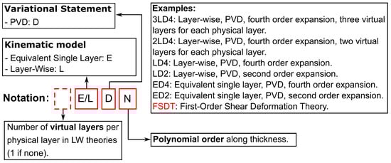
Figure 5. Acronym system.

The initial letter indicates the type of through-thickness representation: E denotes ESL formulations, while L refers to LW descriptions. The second letter identifies the variational approach employed, where D corresponds to PVD. The final digit specifies the polynomial order of the thickness expansion. For LW models, an additional leading digit can appear to define the number of virtual layers introduced for each physical lamina. When such a digit is omitted, a single virtual layer per physical layer is implicitly assumed. The FSDT solution, is obtained through the ED1 model, by reducing the material stiffness matrix accordingly and enforcing the condition $u_{z\tau }=0$ for $\tau =1$.

3. Numerical Results and Discussion

The benchmark problems analyzed in this section consider shells of revolution with three different geometries: a toroid, an ellipsoid and a hyperboloid. Parametric studies are performed considering different values of thickness. Material properties are represented in Table 2, where L and T stand for longitudinal and transverse fibers direction, respectively.

Table 2. Material properties.

Case	${\mathit{E}}_{\mathit{L}}$	${\mathit{E}}_{\mathit{T}}$	${\mathit{G}}_{\mathit{LT}},{\mathit{G}}_{\mathit{TT}}$	${\mathit{\nu }}_{\mathit{LT}},{\mathit{\nu }}_{\mathit{TT}}$	$\mathit{\rho }$
1, 2, 3	50 GPa	10 GPa	5 GPa	$0.25$ GPa	1540 kg/m3

All shells are composed of two layers with the same thickness and they are fully clamped at the extremities. Axes $x^{\prime }$ and $y^{\prime }$ of the local fibers reference system are parallel to $\alpha$ and $\beta$, with their origin $o^{\prime }$ placed in correspondence of $\alpha =l_{\alpha }/2$, $\beta =l_{\beta }/2$. The reference results were obtained using Abaqus 3D simulations, employing C3D20R elements. Because the fiber orientation in Abaqus is assumed constant within individual elements, an adequately fine discretisation over the shell mid-surface was required to ensure accuracy. In contrast, the CUF-based analyses adopted QUAD9 elements. For both modeling approaches, a preliminary mesh sensitivity study was conducted to identify the optimal element density and guarantee convergence of the computed natural frequencies and mode shapes. The percentage error for the i-th frequency is evaluated as follows:

$${\delta }_i={\displaystyle \frac{|F_{i,\mathrm{CUF}}-F_{i,\mathrm{Abaqus}3\mathrm{D}}|}{|F_{i,\mathrm{Abaqus}3\mathrm{D}}|}}·100,$$

(35)

where $F_i$ is the eigenfrequency corresponding to the mode i. In the tables where the comparison between modal frequencies is presented, the percentage errors are reported in round parentheses for each considered theory and eigenmode.

3.1. Toroid

Case 1 involves a bi-layer toroidal shell section with the following dimensions: $R_1=4$ m, $R_2=1$ m, $\alpha \in \left[0,\pi /2\right]$, $\beta \in \left[0,\pi /2\right]$, $l_{\alpha }=\pi /2$ m, $l_{\beta }=\pi /2$ m. The reference systems that have been used to describe the problem are represented in Figure 6. The radius vector is defined as:

$$\mathit{r}=\left\{\begin{array}{c}{R}_{1}cos\left(\beta \right)+R_{2}sin\left(\alpha \right)cos\left(\beta \right)\\ R_{1}sin\left(\beta \right)+R_{2}sin\left(\alpha \right)sin\left(\beta \right)\\ R_{2}cos\left(\alpha \right)\end{array}\right\}.$$

(36)

The following geometrical entities are considered:

$$\begin{array}{c}A=R_2,B=R_1+R_{2}sin\left(\alpha \right),\hfill \\ {\displaystyle \frac{1}{R_{\alpha }}}={\displaystyle \frac{1}{R_2}},{\displaystyle \frac{1}{R_{\beta }}}={\displaystyle \frac{sin\left(\alpha \right)}{R_1+R_{2}sin\left(\alpha \right)}},\hfill \\ H_{\alpha }=R_2(1+\frac{z}{R_2}),H_{\beta }=(R_1+R_2\sin (\alpha ))(1+z\frac{\sin (\alpha )}{R_1+R_2\sin (\alpha )}).\hfill \end{array}$$

(37)

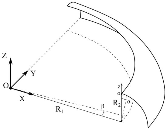
Figure 6. Geometry and reference system, case 1.

It is assumed that fibers angle is function of $y^{\prime }$. Accordingly, the characteristic length in Equation (23) is defined as $d=l_{\beta }/2$. The fiber orientation follows the angular distribution law $\left[90<0,-45>;90<0,45>\right]$. The Abaqus reference model employs 12 elements through the thickness, and 28 and 112 elements along the $\alpha$ and $\beta$ curvilinear directions, respectively.

A preliminary convergence analysis is summarized in Table 3.

Table 3. Comparison of DOF and eigenfrequencies (rad/s$·{10}^2$) between Abaqus 3D and ED2 mesh, $l_{\alpha }/h=10$, case 1.

		Mode
	DOF	$\mathbf{1}\mathbf{(}{\mathit{\delta }}_{\mathbf{1}}\mathbf{\%}\mathbf{)}$	$\mathbf{2}\mathbf{(}{\mathit{\delta }}_{\mathbf{2}}\mathbf{\%}\mathbf{)}$	$\mathbf{3}\mathbf{(}{\mathit{\delta }}_{\mathbf{3}}\mathbf{\%}\mathbf{)}$	$\mathbf{4}\mathbf{(}{\mathit{\delta }}_{\mathbf{4}}\mathbf{\%}\mathbf{)}$	$\mathbf{5}\mathbf{(}{\mathit{\delta }}_{\mathbf{5}}\mathbf{\%}\mathbf{)}$	$\mathbf{6}\mathbf{(}{\mathit{\delta }}_{\mathbf{6}}\mathbf{\%}\mathbf{)}$
ABAQUS 3D	495,843	24.33	25.03	25.22	26.57	26.92	28.21
2 × 8	765	26.15 (7.47)	26.49 (5.82)	28.26 (12.06)	29.63 (11.53)	31.49 (16.98)	32.89 (16.61)
4 × 16	2673	24.66 (1.34)	25.21 (0.72)	25.91 (2.74)	27.22 (2.45)	27.48 (2.08)	28.48 (0.96)
6 × 24	5733	24.50 (0.70)	25.11 (0.33)	25.55 (1.32)	27.04 (1.75)	27.07 (0.55)	28.36 (0.53)
8 × 32	9945	24.47 (0.55)	25.09 (0.24)	25.48 (1.03)	26.95 (1.43)	27.03 (0.42)	28.33 (0.44)

This table presents a comparative assessment of the solutions obtained from Abaqus 3D and ED2, focusing on progressively refined meshes for the case where $l_{\alpha }/h=10$. The second column details the number of Degrees of Freedom (DOF), which is indicative of computational cost. Subsequent columns provide a comparison of the eigenfrequencies derived from both methodologies. It can be observed that mesh refinement leads to results that increasingly converge toward the reference solution for each natural mode. Despite this, increasing the number of elements in the model results in a higher number of DOF, which is directly associated with greater computational cost and longer analysis times. The coarse 2 × 8 mesh, despite its significantly reduced number of DOF, exhibits excessively large percentage errors in the eigenfrequencies and is unable to accurately predict the modal shapes beyond the second mode. The 4 × 16 mesh provides more accurate results but exhibits an inversion between the 4th and 5th modes. Additionally, the error in the first natural frequency exceeds $1.00\%$. This error is significantly reduced when using the 6 × 24 mesh. For the first natural frequency, the percentage errors for the 6 × 24 and 8 × 32 meshes are $0.70\%$ and $0.55\%$, respectively. However, the number of unknowns in the 8 × 32 mesh is $73.47\%$ higher, which is not justifiable given the marginal improvement in computational accuracy. For these reasons, the 6 × 24 mesh is chosen to perform the dynamic analysis in this case.

Table 4 shows the DOF and the eigenfrequencies for various models when $l_{\alpha }/h=5$.

Table 4. DOF and eigenfrequencies (rad/s$·{10}^2$), $l_{\alpha }/h=5$, case 1.

		Mode
	DOF	$\mathbf{1}\mathbf{(}{\mathit{\delta }}_{\mathbf{1}}\mathbf{\%}\mathbf{)}$	$\mathbf{2}\mathbf{(}{\mathit{\delta }}_{\mathbf{2}}\mathbf{\%}\mathbf{)}$	$\mathbf{3}\mathbf{(}{\mathit{\delta }}_{\mathbf{3}}\mathbf{\%}\mathbf{)}$	$\mathbf{4}\mathbf{(}{\mathit{\delta }}_{\mathbf{4}}\mathbf{\%}\mathbf{)}$	$\mathbf{5}\mathbf{(}{\mathit{\delta }}_{\mathbf{5}}\mathbf{\%}\mathbf{)}$	$\mathbf{6}\mathbf{(}{\mathit{\delta }}_{\mathbf{6}}\mathbf{\%}\mathbf{)}$
ABAQUS 3D	495,843	29.11	29.90	32.21	34.54	37.10	37.64
LD4	17,199	29.14 (0.09)	29.94 (0.11)	32.25 (0.14)	34.58 (0.13)	37.23 (0.35)	37.71 (0.19)
LD2	9555	29.16 (0.16)	29.96 (0.20)	32.29 (0.26)	34.632 (0.28)	37.34 (0.66)	37.80 (0.44)
ED6	13,377	29.14 (0.09)	29.94 (0.11)	32.26 (0.14)	34.58 (0.13)	37.23 (0.35)	37.71 (0.19)
ED4	9555	29.14 (0.10)	29.94 (0.12)	32.26 (0.16)	34.59 (0.15)	37.25 (0.41)	37.73 (0.23)
ED2	5733	29.33 (0.78)	30.16 (0.85)	32.53 (1.00)	34.93 (1.15)	37.94 (2.27)	38.41 (2.04)
FSDT	3822	29.21 (0.35)	30.06 (0.54)	32.46 (0.79)	34.91 (1.08)	37.91 (2.18)	38.32 (1.81)

In all CUF models, a significant reduction in the number of unknowns is observed compared to Abaqus 3D, which has a number of DOF at least two orders of magnitude higher. CUF models are characterized by a lower number of DOF and demonstrate the ability to achieve progressively more accurate results with higher-order expansions along the thickness, while all CUF models can correctly predict the modal shapes of the reference solution, the ED2 and FSDT theories provide the least accurate approximation of eigenfrequencies. This is because, in the case of a thick shell, the order of the $F_{\tau }$ functions significantly influences the prediction of the displacement field along the thickness. This is confirmed by ED6 and LD4 results, which show the lowest percentage errors for the first frequency, corresponding to $0.09\%$.

For higher frequencies, the LD4 theory gives a better approximation than the ED6 model, because in thick, multilayered shells, independently representing the kinematics of each layer becomes essential. Table 5 shows the same eigenfrequencies in the case $l_{\alpha }/h=10$. Since a slightly thinner shell is considered, lower-order theories are closer to the reference solution. ED2 and FSDT models exhibit similar approximations, with the highest percentage error of $1.75\%$ and $1.43\%$, respectively, corresponding to the 4th mode. For the same mode, the best result is obtained through LD4 which shows a percentage error of $0.62\%$. The corresponding modal shapes are represented in Figure 7, where the ED2 solution is compared with the Abaqus 3D reference. In both the CUF-based and Abaqus solutions, the eigenvectors are normalized so that the maximum displacement magnitude of each mode shape equals one. The same scaling factor is consistently applied across all the presented mode shapes for visual comparison. The figure demonstrates good agreement between the ESL CUF second-order model and the reference solution across all modes. It can be observed that lower frequencies correspond to fewer semi-waves along the $\alpha$ and $\beta$ axes, starting with one semi-wave for the first frequency. Higher frequencies are associated with more complex modes, displaying more semi-waves, as seen in the sixth mode, where four semi-waves are visible. Table 6 shows the eigenfrequencies in the case $l_{\alpha }/h=100$.

Table 5. Eigenfrequencies (rad/s$·{10}^2$), $l_{\alpha }/h=10$, case 1.

	Mode
	$\mathbf{1}\mathbf{(}{\mathit{\delta }}_{\mathbf{1}}\mathbf{\%}\mathbf{)}$	$\mathbf{2}\mathbf{(}{\mathit{\delta }}_{\mathbf{2}}\mathbf{\%}\mathbf{)}$	$\mathbf{3}\mathbf{(}{\mathit{\delta }}_{\mathbf{3}}\mathbf{\%}\mathbf{)}$	$\mathbf{4}\mathbf{(}{\mathit{\delta }}_{\mathbf{4}}\mathbf{\%}\mathbf{)}$	$\mathbf{5}\mathbf{(}{\mathit{\delta }}_{\mathbf{5}}\mathbf{\%}\mathbf{)}$	$\mathbf{6}\mathbf{(}{\mathit{\delta }}_{\mathbf{6}}\mathbf{\%}\mathbf{)}$
ABAQUS 3D	24.33	25.03	25.22	26.57	26.92	28.21
LD4	24.41 (0.31)	25.07 (0.16)	25.33 (0.46)	26.73 (0.61)	26.98 (0.24)	28.27 (0.21)
LD2	24.42 (0.36)	25.07 (0.18)	25.35 (0.54)	26.77 (0.75)	26.99 (0.27)	28.28 (0.25)
ED6	24.41 (0.31)	25.07 (0.16)	25.33 (0.46)	26.73 (0.61)	26.98 (0.24)	28.27 (0.22)
ED4	24.41 (0.32)	25.07 (0.16)	25.34 (0.48)	26.74 (0.64)	26.98 (0.24)	28.27 (0.22)
ED2	24.50 (0.70)	25.111 (0.33)	25.55 (1.32)	27.04 (1.75)	27.07 (0.55)	28.36 (0.53)
FSDT	24.45 (0.49)	25.09 (0.22)	25.47 (1.02)	26.95 (1.43)	27.04 (0.45)	28.35 (0.49)

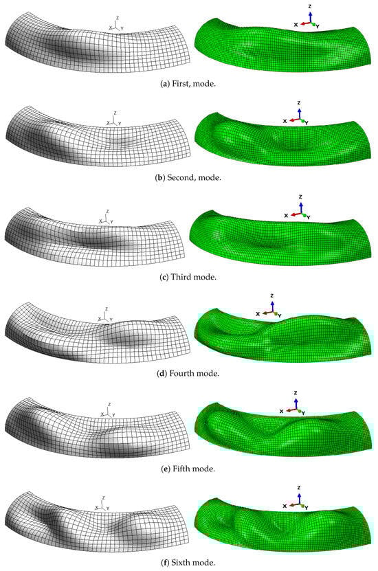
Figure 7. Modal shapes, comparison between ED2 model (left) and Abaqus 3D (right), $l_{\alpha }/h=10$, case 1.

Table 6. Eigenfrequencies (rad/s$·{10}^2$), $l_{\alpha }/h=100$, case 1.

	Mode
	$\mathbf{1}\mathbf{(}{\mathit{\delta }}_{\mathbf{1}}\mathbf{\%}\mathbf{)}$	$\mathbf{2}\mathbf{(}{\mathit{\delta }}_{\mathbf{2}}\mathbf{\%}\mathbf{)}$	$\mathbf{3}\mathbf{(}{\mathit{\delta }}_{\mathbf{3}}\mathbf{\%}\mathbf{)}$	$\mathbf{4}\mathbf{(}{\mathit{\delta }}_{\mathbf{4}}\mathbf{\%}\mathbf{)}$	$\mathbf{5}\mathbf{(}{\mathit{\delta }}_{\mathbf{5}}\mathbf{\%}\mathbf{)}$	$\mathbf{6}\mathbf{(}{\mathit{\delta }}_{\mathbf{6}}\mathbf{\%}\mathbf{)}$
ABAQUS 3D	8.47	9.35	9.37	9.83	10.55	11.26
LD4	8.51 (0.47)	9.43 (0.85)	9.47 (1.14)	9.91 (0.88)	10.66 (1.05)	11.43 (1.52)
LD2	8.51 (0.47)	9.43 (0.85)	9.47 (1.14)	9.91 (0.88)	10.66 (1.05)	11.43 (1.52)
ED6	8.51 (0.47)	9.43 (0.85)	9.47 (1.14)	9.91 (0.88)	10.66 (1.05)	11.43 (1.52)
ED4	8.51 (0.47)	9.43 (0.85)	9.47 (1.14)	9.91 (0.88)	10.66 (1.05)	11.43 (1.52)
ED2	8.51 (0.48)	9.43 (0.86)	9.47 (1.16)	9.92 (0.89)	10.66 (1.06)	11.43 (1.54)
FSDT	8.50 (0.40)	9.42 (0.75)	9.46 (1.03)	9.91 (0.82)	10.65 (0.96)	11.42 (1.47)

Since a thin shell is considered, the expansion order of the z-dependent functions has limited importance in predicting the displacement field behavior. In this case, a linear law is sufficient to represent the displacements along the thickness, and the various CUF-based theories provide similar approximation levels to the reference solution, both in terms of frequencies and modal shapes. CUF theories show a maximum error of $1.54\%$ in correspondence of the sixth frequency and a minimum error of $0.40\%$ on the first frequency. It can be observed that as the side-to-thickness ratio increases, the frequencies decrease due to the reduced thickness of the analyzed shells.

3.2. Ellipsoid

A shell with two layers and an ellipsoidal mid-surface is studied as second case. The equation of the middle surface can be written in Cartesian coordinates as follows:

$${\displaystyle \frac{X^2}{a^2}}+{\displaystyle \frac{Y^2}{b^2}}+{\displaystyle \frac{Z^2}{c^2}}=1.$$

(38)

The following dimensions are considered: $a=c=1$ m, $b=4$ m, $\alpha \in \left[0,\pi /2\right]$, $\beta \in \left[0,\pi /4\right]$, $l_{\alpha }=\pi /2$ m, $l_{\beta }=\pi /4$ m. The geometry and the reference systems that have been used to describe the problem are shown in Figure 8. The radius vector is defined as:

$$\mathit{r}=\left\{\begin{array}{c}asin\left(\alpha \right)cos\left(\beta \right)\\ bsin\left(\beta \right)\\ acos\left(\alpha \right)cos\left(\beta \right)\end{array}\right\}.$$

(39)

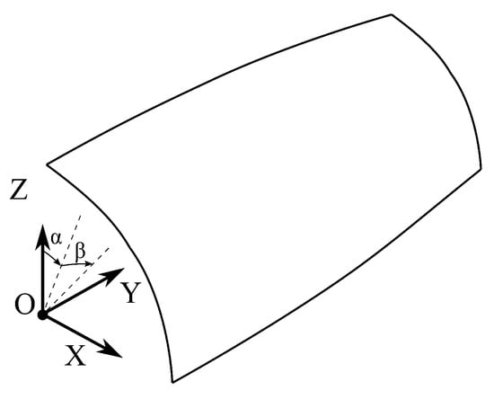
Figure 8. Geometry and reference system, case 2.

The following geometrical entities are considered:

$$\begin{array}{c}A=acos\left(\beta \right),B=\sqrt{a^{2}sin{\left(\beta \right)}^2+b^{2}cos{\left(\beta \right)}^2},\hfill \\ {\displaystyle \frac{1}{R_{\alpha }}}={\displaystyle \frac{b}{a\sqrt{a^{2}sin{\left(\beta \right)}^2+b^{2}cos{\left(\beta \right)}^2}}},{\displaystyle \frac{1}{R_{\beta }}}={\displaystyle \frac{ab}{{\left(a^{2}sin{\left(\beta \right)}^2+b^{2}cos{\left(\beta \right)}^2\right)}^{3/2}}},\hfill \\ H_{\alpha }=acos\left(\beta \right)\left(1+z{\displaystyle \frac{b}{a\sqrt{a^{2}sin{\left(\beta \right)}^2+b^{2}cos{\left(\beta \right)}^2}}}\right),\hfill \\ H_{\beta }=\sqrt{a^{2}sin{\left(\beta \right)}^2+b^{2}cos{\left(\beta \right)}^2}\left(1+z{\displaystyle \frac{ab}{{\left(a^{2}sin{\left(\beta \right)}^2+b^{2}cos{\left(\beta \right)}^2\right)}^{3/2}}}\right).\hfill \end{array}$$

(40)

It is assumed that fibers angle is function of $x^{\prime }$. Therefore the characteristic length of Equation (23) is set to $d=l_{\alpha }/2$. Angle variational law is expressed as $\left[0<0,-45>;0<0,45>\right]$. The reference solution in Abaqus employs a mesh with 60 elements along the $\alpha$ direction, 120 elements along $\beta$, and 12 elements through the thickness. For the CUF simulations, a discretisation of 9 elements along $\alpha$ and 18 elements along $\beta$ is adopted. This choice follows a convergence test similar to the one presented in the first case, which is omitted here for the sake of conciseness. Table 7 shows the eigenfrequencies, in the case of a thick shell, where $l_{\alpha }/h=5$.

Table 7. Eigenfrequencies (rad/s$·{10}^2$), $l_{\alpha }/h=5$, case 2.

	Mode
	$\mathbf{1}\mathbf{(}{\mathit{\delta }}_{\mathbf{1}}\mathbf{\%}\mathbf{)}$	$\mathbf{2}\mathbf{(}{\mathit{\delta }}_{\mathbf{2}}\mathbf{\%}\mathbf{)}$	$\mathbf{3}\mathbf{(}{\mathit{\delta }}_{\mathbf{3}}\mathbf{\%}\mathbf{)}$	$\mathbf{4}\mathbf{(}{\mathit{\delta }}_{\mathbf{4}}\mathbf{\%}\mathbf{)}$	$\mathbf{5}\mathbf{(}{\mathit{\delta }}_{\mathbf{5}}\mathbf{\%}\mathbf{)}$	$\mathbf{6}\mathbf{(}{\mathit{\delta }}_{\mathbf{6}}\mathbf{\%}\mathbf{)}$
ABAQUS 3D	48.90	50.89	54.52	58.61	61.81	62.36
LD4	48.95 (0.10)	50.94 (0.10)	54.57 (0.10)	58.67 (0.11)	61.89 (0.12)	62.48 (0.19)
LD2	49.034 (0.29)	51.33 (0.87)	54.73 (0.39)	59.01 (0.69)	62.05 (0.38)	62.64 (0.44)
ED6	48.95 (0.11)	50.95 (0.11)	54.57 (0.11)	58.68 (0.12)	61.90 (0.13)	62.49 (0.21)
ED4	48.97 (0.14)	51.06 (0.32)	54.61 (0.17)	58.77 (0.28)	61.94 (0.21)	62.53 (0.27)
ED2	49.55 (1.33)	52.52 (3.19)	55.55 (1.89)	60.08 (2.52)	62.85 (1.68)	63.96 (2.56)
FSDT	49.47 (1.18)	52.56 (3.27)	55.60 (2.00)	60.10 (2.55)	62.85 (1.68)	64.13 (2.83)

In this case, the best approximation is given by the LD4 model, which shows a maximum error of $0.10\%$ for the second modal frequency. The differences between the LW and ESL theories are more pronounced in this case. Comparing the ED6 and LD4 models, it can be observed that the latter provides a better approximation, despite using a lower order of expansion along the z-axis. The ED2 and FSDT models show the least accurate approximations, while FSDT is more accurate for the first modal frequency, its percentage error increases progressively with higher frequencies, whereas the ED2 theory offers a more consistent overall approximation. Table 8 considers the eigenfrequencies for the case $l_{\alpha }/h=10$.

Table 8. Eigenfrequencies (rad/s$·{10}^2$), $l_{\alpha }/h=10$, case 2.

	Mode
	$\mathbf{1}\mathbf{(}{\mathit{\delta }}_{\mathbf{1}}\mathbf{\%}\mathbf{)}$	$\mathbf{2}\mathbf{(}{\mathit{\delta }}_{\mathbf{2}}\mathbf{\%}\mathbf{)}$	$\mathbf{3}\mathbf{(}{\mathit{\delta }}_{\mathbf{3}}\mathbf{\%}\mathbf{)}$	$\mathbf{4}\mathbf{(}{\mathit{\delta }}_{\mathbf{4}}\mathbf{\%}\mathbf{)}$	$\mathbf{5}\mathbf{(}{\mathit{\delta }}_{\mathbf{5}}\mathbf{\%}\mathbf{)}$	$\mathbf{6}\mathbf{(}{\mathit{\delta }}_{\mathbf{6}}\mathbf{\%}\mathbf{)}$
ABAQUS 3D	38.38	43.29	45.61	47.37	51.96	53.35
LD4	38.47 (0.22)	43.33 (0.09)	45.70 (0.18)	47.40 (0.08)	52.00 (0.09)	53.45 (0.18)
LD2	38.62 (0.63)	43.38 (0.20)	45.86 (0.54)	47.45 (0.17)	52.06 (0.19)	53.62 (0.51)
ED6	38.47 (0.22)	43.33 (0.09)	45.70 (0.19)	47.41 (0.08)	52.00 (0.09)	53.45 (0.19)
ED4	38.50 (0.30)	43.34 (0.12)	45.73 (0.25)	47.41 (0.10)	52.01 (0.11)	53.48 (0.24)
ED2	39.35 (2.52)	43.63 (0.79)	46.63 (2.23)	47.73 (0.75)	52.40 (0.85)	54.47 (2.10)
FSDT	39.37 (2.57)	43.60 (0.71)	46.69 (2.35)	47.74 (0.79)	52.43 (0.91)	54.55 (2.24)

The decrease in the shell thickness allows to reduce lower-order theories errors, as shown by ED2 and FSDT models which now show similar accuracy in frequencies prediction. The FSDT model is still showing the worst level of accuracy, with a maximum error of $2.57\%$ in correspondence of the first frequency. Considering the same mode, the error can be reduced to a minimum of $0.22\%$ with the LD4 model. Figure 9 shows the modal shapes obtained with the ED2 model, which have been compared with the reference shapes from Abaqus, demonstrating good agreement. This comparison is not reported here for brevity. Table 9 shows the eigenfrequencies for $l_{\alpha }/h=100$.

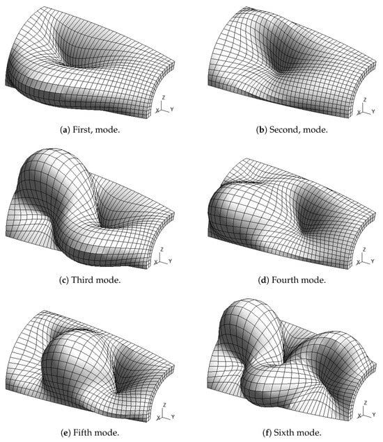
Figure 9. Modal shapes, ED2 model, $l_{\alpha }/h=10$, case 2.

Table 9. Eigenfrequencies (rad/s$·{10}^2$), $l_{\alpha }/h=100$, case 2.

	Mode
	$\mathbf{1}\mathbf{(}{\mathit{\delta }}_{\mathbf{1}}\mathbf{\%}\mathbf{)}$	$\mathbf{2}\mathbf{(}{\mathit{\delta }}_{\mathbf{2}}\mathbf{\%}\mathbf{)}$	$\mathbf{3}\mathbf{(}{\mathit{\delta }}_{\mathbf{3}}\mathbf{\%}\mathbf{)}$	$\mathbf{4}\mathbf{(}{\mathit{\delta }}_{\mathbf{4}}\mathbf{\%}\mathbf{)}$	$\mathbf{5}\mathbf{(}{\mathit{\delta }}_{\mathbf{5}}\mathbf{\%}\mathbf{)}$	$\mathbf{6}\mathbf{(}{\mathit{\delta }}_{\mathbf{6}}\mathbf{\%}\mathbf{)}$
ABAQUS 3D	9.09	10.64	13.55	14.15	17.02	17.46
LD4	9.12 (0.27)	10.73 (0.83)	13.63 (0.64)	14.25 (0.71)	17.11 (0.55)	17.63 (0.93)
LD2	9.12 (0.27)	10.73 (0.84)	13.63 (0.65)	14.25 (0.72)	17.11 (0.56)	17.63 (0.93)
ED6	9.12 (0.27)	10.73 (0.83)	13.63 (0.64)	14.25 (0.71)	17.11 (0.55)	17.63 (0.93)
ED4	9.12 (0.27)	10.73 (0.83)	13.63 (0.64)	14.25 (0.71)	17.11 (0.55)	17.63 (0.93)
ED2	9.12 (0.30)	10.73 (0.89)	13.64 (0.70)	14.26 (0.76)	17.12 (0.61)	17.64 (1.00)
FSDT	9.12 (0.26)	10.72 (0.73)	13.63 (0.62)	14.25 (0.73)	17.11 (0.56)	17.63 (0.94)

In this case, classical and lower-order theories are sufficient to match the modal frequencies of the reference solution due to the thin shell being considered. For instance, the FSDT closely approximates the reference solution for the first three modes, but its percentage error increases thereafter, reaching a maximum of $0.94\%$ for the sixth frequency. Additionally, the difference between the LD4 and ED6 theories is not significant, as all the proposed theories demonstrate good approximation.

3.3. Hyperboloid

Case 3 studies a hyperboloid characterized by two plies. The equation of the middle surface can be written in Cartesian coordinates as follows:

$${\displaystyle \frac{X^2}{a^2}}-{\displaystyle \frac{Y^2}{b^2}}+{\displaystyle \frac{Z^2}{c^2}}=1.$$

(41)

The following dimensions are considered: $a=c=1$ m, $b=4$, $\alpha \in \left[0,\pi /2\right]$, $\beta \in \left[0,\pi /4\right]$, $l_{\alpha }=\pi /2$ m, $l_{\beta }=\pi /4$ m. The geometry and reference systems of this case are shown in Figure 10. The radius vector is defined as:

$$\mathit{r}=\left\{\begin{array}{c}asin\left(\alpha \right)cosh\left(\beta \right)\\ bsinh\left(\beta \right)\\ acos\left(\alpha \right)cosh\left(\beta \right)\end{array}\right\}.$$

(42)

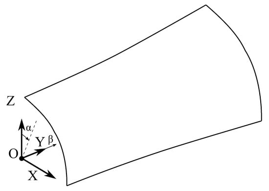
Figure 10. Geometry and reference system, case 3.

The following geometrical entities are considered:

$$\begin{array}{c}A=acosh\left(\beta \right),B=\sqrt{a^{2}sinh{\left(\beta \right)}^2+b^{2}cosh{\left(\beta \right)}^2}.\hfill \\ {\displaystyle \frac{1}{R_{\alpha }}}={\displaystyle \frac{b}{a\sqrt{a^{2}sinh{\left(\beta \right)}^2+b^{2}cosh{\left(\beta \right)}^2}}},{\displaystyle \frac{1}{R_{\beta }}}={\displaystyle \frac{-ab}{{\left(a^{2}sinh{\left(\beta \right)}^2+b^{2}cosh{\left(\beta \right)}^2\right)}^{3/2}}}.\hfill \\ H_{\alpha }=acosh\left(\beta \right)\left(1+z{\displaystyle \frac{b}{a\sqrt{a^{2}sinh{\left(\beta \right)}^2+b^{2}cosh{\left(\beta \right)}^2}}}\right),\hfill \\ H_{\beta }=\sqrt{a^{2}sinh{\left(\beta \right)}^2+b^{2}cosh{\left(\beta \right)}^2}\left(1+z{\displaystyle \frac{-ab}{{\left(a^{2}sinh{\left(\beta \right)}^2+b^{2}cosh{\left(\beta \right)}^2\right)}^{3/2}}}\right).\hfill \end{array}$$

(43)

The same fiber angle variation as in the previous case is adopted. The Abaqus reference model employs a mesh of 60 elements along $\alpha$, 120 elements along $\beta$, and 12 elements through the thickness, whereas the CUF simulations use 9 elements along $\alpha$ and 18 elements along $\beta$. The eigenfrequencies for $l_{\alpha }/h=5$ are presented in Table 10.

Table 10. Eigenfrequencies (rad/s$·{10}^2$), $l_{\alpha }/h=5$, case 3.

	Mode
	$\mathbf{1}\mathbf{(}{\mathit{\delta }}_{\mathbf{1}}\mathbf{\%}\mathbf{)}$	$\mathbf{2}\mathbf{(}{\mathit{\delta }}_{\mathbf{2}}\mathbf{\%}\mathbf{)}$	$\mathbf{3}\mathbf{(}{\mathit{\delta }}_{\mathbf{3}}\mathbf{\%}\mathbf{)}$	$\mathbf{4}\mathbf{(}{\mathit{\delta }}_{\mathbf{4}}\mathbf{\%}\mathbf{)}$	$\mathbf{5}\mathbf{(}{\mathit{\delta }}_{\mathbf{5}}\mathbf{\%}\mathbf{)}$	$\mathbf{6}\mathbf{(}{\mathit{\delta }}_{\mathbf{6}}\mathbf{\%}\mathbf{)}$
ABAQUS 3D	39.09	40.62	43.53	46.29	48.18	52.66
LD4	39.11 (0.06)	40.69 (0.19)	43.56 (0.07)	46.36 (0.14)	48.22 (0.08)	52.70 (0.07)
LD2	39.17 (0.20)	40.98 (0.88)	43.64 (0.26)	46.60 (0.66)	48.38 (0.43)	52.87 (0.40)
ED6	39.11 (0.07)	40.70 (0.20)	43.56 (0.07)	46.36 (0.14)	48.22 (0.09)	52.70 (0.08)
ED4	39.12 (0.09)	40.76 (0.36)	43.58 (0.11)	46.42 (0.27)	48.25 (0.15)	52.75 (0.17)
ED2	39.51 (1.07)	41.99 (3.38)	44.13 (1.38)	47.43 (2.46)	49.27 (2.26)	53.52 (1.64)
FSDT	39.46 (0.96)	42.01 (3.44)	44.14 (1.40)	47.40 (2.40)	49.39 (2.53)	53.52 (1.63)

The highest error is shown by the FSDT model for the second natural frequency and it is equal to $3.44\%$. A noticeable improvement is achieved with the ED6 and LD4 models, which show errors of $0.20\%$ and $0.19\%$, respectively, for the same frequency. In this case, the LD4 model provides the best approximation, as it represents the displacement field using fourth-order polynomials for each layer of the shell. This explains why the LD4 model outperforms the ED6 model, despite the latter having a higher order of expansion along the thickness. For $l_{\alpha }/h=10$, the eigenfrequencies are displayed in Table 11.

Table 11. Eigenfrequencies (rad/s$·{10}^2$), $l_{\alpha }/h=10$, case 3.

	Mode
	$\mathbf{1}\mathbf{(}{\mathit{\delta }}_{\mathbf{1}}\mathbf{\%}\mathbf{)}$	$\mathbf{2}\mathbf{(}{\mathit{\delta }}_{\mathbf{2}}\mathbf{\%}\mathbf{)}$	$\mathbf{3}\mathbf{(}{\mathit{\delta }}_{\mathbf{3}}\mathbf{\%}\mathbf{)}$	$\mathbf{4}\mathbf{(}{\mathit{\delta }}_{\mathbf{4}}\mathbf{\%}\mathbf{)}$	$\mathbf{5}\mathbf{(}{\mathit{\delta }}_{\mathbf{5}}\mathbf{\%}\mathbf{)}$	$\mathbf{6}\mathbf{(}{\mathit{\delta }}_{\mathbf{6}}\mathbf{\%}\mathbf{)}$
ABAQUS 3D	28.96	33.90	34.55	37.88	39.43	40.93
LD4	29.05 (0.32)	33.99 (0.24)	34.62 (0.20)	37.95 (0.17)	39.51 (0.19)	40.99 (0.14)
LD2	29.14 (0.63)	34.06 (0.47)	34.68 (0.36)	37.98 (0.26)	39.61 (0.44)	41.02 (0.23)
ED6	29.06 (0.32)	33.99 (0.25)	34.62 (0.20)	37.95 (0.17)	39.51 (0.20)	40.99 (0.15)
ED4	29.07 (0.38)	34.00 (0.29)	34.63 (0.23)	37.95 (0.19)	39.53 (0.24)	40.99 (0.16)
ED2	29.58 (2.15)	34.39 (1.44)	35.04 (1.41)	38.18 (0.80)	40.11 (1.72)	41.26 (0.82)
FSDT	29.57 (2.11)	34.35 (1.32)	35.06 (1.48)	38.17 (0.76)	40.13 (1.77)	41.28 (0.86)

As discussed earlier, classical and low-order theories generally struggle to accurately capture eigenfrequencies when the side-to-thickness ratio is low. In contrast, layer-wise theories demonstrate superior accuracy, closely aligning with the Abaqus solution, particularly at higher frequencies.

Despite this, FSDT is still able to predict the modal shapes correctly and shows errors strictly lower than $2.20\%$. The best approximation is still given by the LD4 model. The modal shapes obtained through the ED2 model for $l_{\alpha }/h=10$ are shown in Figure 11. The obtained shapes agree with the Abaqus results, which are not shown here to maintain conciseness.

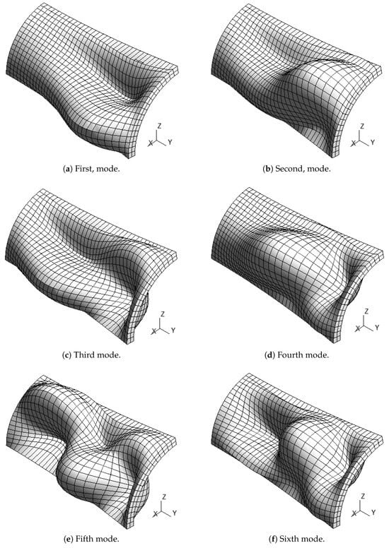
Figure 11. Modal shapes, ED2 model, $l_{\alpha }/h=10$, case 3.

Table 12 provides the eigenfrequencies for $l_{\alpha }/h=100$. As already observed in the previous cases, all the proposed theories show a good approximation of Abaqus 3D results. This is because, in thin shells, the displacement variation across the thickness is minimal, and a simple linear or low-order representation is sufficient to capture the kinematic behavior. The reduced complexity of the displacement field along the thickness means that higher-order terms contribute little to improving accuracy, allowing lower-order models to effectively approximate the modal behavior. However, in this case CUF models errors do not exceed the value of $1.00\%$.

Table 12. Eigenfrequencies (rad/s$·{10}^2$), $l_{\alpha }/h=100$, case 3.

	Mode
	$\mathbf{1}\mathbf{(}{\mathit{\delta }}_{\mathbf{1}}\mathbf{\%}\mathbf{)}$	$\mathbf{2}\mathbf{(}{\mathit{\delta }}_{\mathbf{2}}\mathbf{\%}\mathbf{)}$	$\mathbf{3}\mathbf{(}{\mathit{\delta }}_{\mathbf{3}}\mathbf{\%}\mathbf{)}$	$\mathbf{4}\mathbf{(}{\mathit{\delta }}_{\mathbf{4}}\mathbf{\%}\mathbf{)}$	$\mathbf{5}\mathbf{(}{\mathit{\delta }}_{\mathbf{5}}\mathbf{\%}\mathbf{)}$	$\mathbf{6}\mathbf{(}{\mathit{\delta }}_{\mathbf{6}}\mathbf{\%}\mathbf{)}$
ABAQUS 3D	7.10	7.55	9.38	10.08	11.82	12.23
LD4	7.11 (0.24)	7.61 (0.79)	9.44 (0.62)	10.16 (0.85)	11.88 (0.52)	12.33 (0.85)
LD2	7.11 (0.25)	7.61 (0.81)	9.44 (0.62)	10.16 (0.85)	11.88 (0.52)	12.33 (0.86)
ED6	7.11 (0.24)	7.61 (0.79)	9.44 (0.62)	10.16 (0.85)	11.88 (0.52)	12.33 (0.85)
ED4	7.11 (0.24)	7.61 (0.79)	9.44 (0.62)	10.16 (0.85)	11.88 (0.52)	12.33 (0.85)
ED2	7.12 (0.27)	7.62 (0.85)	9.44 (0.66)	10.17 (0.90)	11.88 (0.55)	12.34 (0.91)
FSDT	7.11 (0.23)	7.60 (0.65)	9.43 (0.53)	10.16 (0.80)	11.88 (0.49)	12.33 (0.82)

4. Conclusions

This paper presents a numerical approach for the dynamic analysis of VAT shells of revolution. CUF has been implemented within a FEM framework, enabling the derivation of multiple theories by treating the through-the-thickness expansion order as a free parameter. This allows for the development of models with varying levels of accuracy within a unified formulation. The proposed models demonstrate a reduction of more than $90\%$ in the total number of degrees of freedom compared to the reference 3D model. The governing equations for the dynamic problem are derived via the PVD, with displacements considered as the primary variables. The fiber angle follows a linear variation, although the formulation is sufficiently general to accommodate more complex fiber patterns, highlighting the versatility and adaptability of the proposed method. The primary innovation of this work lies in the adaptation of CUF to shells with variable curvature radii, whose dynamic behavior is analyzed using FEM. To account for the curvature variations in the mid-surface, the components of the stiffness matrix FN have been reformulated by incorporating the effects of mid-surface curvature and the coefficients of the first fundamental form. Three case studies are presented, involving shells with toroidal, ellipsoidal, and hyperboloid mid-surfaces, each featuring variable thickness. The following key observations can be obtained from the analysis of the results:

• The FSDT model provides accurate results for thin shells ($l_{\alpha }/h=100$). However, its accuracy diminishes considerably for thicker shells ($l_{\alpha }/h=10$ and 5), especially at higher frequencies. Despite this, the model is capable of accurately predicting the modal shapes in all cases and offers reduced computational cost due to its consideration of a limited number of variables.
• ESL and LW models accurately predict the fundamental frequencies, regardless of the analysis case or shell thickness. For thick plates ($l_{\alpha }/h=5$), these models outperform the FSDT in terms of accuracy. However, higher-order models introduce more variables as additional terms in the thickness expansion functions, enriching the solution by capturing more complex displacement field features.
• The differences between the ESL and LW models become more pronounced when analyzing thick, multilayered shells. In such cases, the independent representation of each layer kinematics is crucial for accurately estimating the composite dynamic behavior. For thin shells, both approaches yield results in good agreement with the Abaqus 3D reference model, independent of the expansion order. However, for thicker shells, higher-order polynomials are required to achieve accurate results. The proposed LW and ESL theories (including FSDT) exhibit average frequency shift errors of $0.45\%$ and $0.84\%$, respectively, resulting in an overall mean error of $0.71\%$ across all proposed models.

The proposed approach does not impose specific constraints on the shell slenderness ratio, thereby enabling the analysis of both thin and thick structures within a unified framework. However, convergence issues may arise when thin shells are modeled using high-order polynomial functions through the thickness. This behavior is well known in numerical methods employing Lagrange polynomials with equally spaced nodes, where oscillations tend to appear near the boundaries of the interpolation interval as the polynomial degree increases. Although such effects are generally negligible in free vibration analyses, where global quantities such as eigenfrequencies and mode shapes are of primary interest, they become more apparent when examining local response quantities, such as stresses or displacements at specific points within the structure. These undesirable numerical effects can be alleviated by adopting a denser distribution of nodes near the boundaries of the polynomial domain. No significant limitations were observed concerning curvature variations, provided that a sufficiently refined mesh is employed along the principal directions of the mid-surface in regions of high curvature gradients. In general, lower curvatures tend to reduce the severity of shear locking, which becomes more noticeable in highly curved structures. Nevertheless, the use of the MITC approach effectively mitigates this phenomenon, ensuring stable and accurate results even in cases involving pronounced curvature variations. The proposed methodology can be realistically extended to shells with non-revolution geometries, although this would require adopting more general surface parametrizations and reference frames. Furthermore, the same framework can be applied to static and buckling analyses, and it could be adapted to account for time-dependent or dynamic boundary conditions in future developments. Potential prospects also foresee the development of more complex variational statements, like the RMVT, within this framework. In the present study, linear free vibration analysis are considered, and therefore, at this stage, the proposed method does not account for geometric or material nonlinearities. The method, however, can be extended to nonlinear regimes by incorporating higher-order displacement-strain-stress relations within the unified formulation, as already demonstrated in the literature CUF-based nonlinear studies. The application of the unified formulation to large-scale industrial geometries is possible, even if specific adaptation techniques should be taken into account to assure the method effectiveness. The CUF-based approach is computationally more demanding than conventional shell elements due to the richer kinematic representation. Nevertheless, its hierarchical nature allows the user to tailor the model complexity to the problem at hand, making it suitable for both academic and industrial-scale analyses when implemented efficiently. In static analysis, global–local modeling can be employed to obtain a coarse global solution and subsequently enhance accuracy in specific regions of the structural domain. Similarly, for free vibration analyses, analogous strategies can be adopted by coupling the CUF with a coarser global mesh to achieve a refined kinematic representation in regions of particular interest. Among these approaches, substructuring techniques and component mode synthesis methods represent effective and widely applicable options.

References

- Xu, P.; Guo, W.; Yang, L.; Yang, C.; Zhou, S. Crashworthiness analysis and multi-objective optimization of a novel metal/CFRP hybrid friction structures. Struct. Multidiscip. Optim. 2024, 67, 97. [Google Scholar] [CrossRef]
- Reddy, J.N. Mechanics of Laminated Composite Plates and Shells: Theory and Analysis; CRC Press: Boca Raton, FL, USA, 2003. [Google Scholar]
- Kraus, H. Thin Elastic Shells: An Introduction to the Theoretical Foundations and the Analysis of Their Static and Dynamic Behavior; John Wiley & Sons: Hoboken, NJ, USA, 1967. [Google Scholar]
- Leissa, A.W. Vibration of Shells; Scientific and Technical Information Office, National Aeronautics and Space Administration: Hampton, VA, USA, 1973. [Google Scholar]
- Bathe, K.-J. Finite Element Procedures; Klaus-Jurgen Bathe: Watertown, MA, USA, 2006. [Google Scholar]
- Washizu, K. Variational Methods in Elasticity and Plasticity; Pergamon Press: Oxford, UK, 1974. [Google Scholar]
- Chung, H. Free vibration analysis of circular cylindrical shells. J. Sound Vib. 1981, 74, 331–350. [Google Scholar] [CrossRef]
- Narita, Y.; Leissa, A. Vibrations of Completely Free Shallow Shells of Curvilinear Planform. J. Appl. Mech. 1986, 53, 647–651. [Google Scholar] [CrossRef]
- Liew, K.M.; Lim, C.W. Vibration of perforated doubly-curved shallow shells with rounded corners. Int. J. Solids Struct. 1994, 31, 1519–1536. [Google Scholar] [CrossRef]
- Chao, C.C.; Tung, T.P. Step pressure and blast responses of clamped orthotropic hemispherical shells. Int. J. Impact Eng. 1989, 8, 191–207. [Google Scholar] [CrossRef]
- Yang, C.; Jin, G.; Zhang, Y.; Liu, Z. A unified three-dimensional method for vibration analysis of the fre-quency-dependent sandwich shallow shells with general boundary conditions. Appl. Math. Model. 2019, 66, 59–76. [Google Scholar] [CrossRef]
- Aksu, T. A finite element formulation for free vibration analysis of shells of general shape. Comput. Struct. 1997, 65, 687–694. [Google Scholar] [CrossRef]
- Chakravorty, D.; Sinha, P.K.; Bandyopadhyay, J.N. Applications of FEM on free and forced vibration of laminated shells. J. Eng. Mech. 1998, 124, 1–8. [Google Scholar] [CrossRef]
- Chaubey, A.K.; Kumar, A.; Chakrabarti, A. Vibration of laminated composite shells with cutouts and con-centrated mass. AIAA J. 2018, 56, 1662–1678. [Google Scholar] [CrossRef]
- Maksymyuk, V.A. Locking phenomenon in computational methods of the shell theory. Int. J. Appl. Mech. 2020, 56, 347–350. [Google Scholar] [CrossRef]
- Bathe, K.-J.; Dvorkin, E.N. A formulation of general shell elements—The use of mixed interpolation of ten-sorial components. Int. J. Numer. Methods Eng. 1986, 22, 697–722. [Google Scholar] [CrossRef]
- Carrera, E. Theories and finite elements for multilayered plates and shells: A unified compact formulation with numerical assessment and benchmarking. Arch. Comput. Methods Eng. 2003, 10, 215–296. [Google Scholar] [CrossRef]
- Carrera, E.; Giunta, G.; Brischetto, S. Hierarchical closed form solutions for plates bent by localized transverse loadings. J. Zhejiang Univ.-Sci. A 2007, 8, 1026–1037. [Google Scholar] [CrossRef]
- Carrera, E.; Campisi, C.; Cinefra, M.; Soave, M. Evaluation of various trough the thickness and curvature approximations for free vibrational analysis of cylindrical and spherical shells. Int. J. Signal Imaging Syst. Eng. 2008, 1, 197. [Google Scholar]
- Giunta, G.; Biscani, F.; Belouettar, S.; Carrera, E. Hierarchical modelling of doubly curved laminated com-posite shells under distributed and localised loadings. Compos. B Eng. 2011, 42, 682–691. [Google Scholar] [CrossRef]
- Giunta, G.; Metla, N.; Belouettar, S.; Ferreira, A.J.M.; Carrera, E. A thermo-mechanical analysis of isotropic and composite beams via collocation with radial basis functions. J. Therm. Stress. 2013, 36, 1169–1199. [Google Scholar] [CrossRef]
- De Pietro, G.; Giunta, G.; Belouettar, S.; Carrera, E. A static analysis of three-dimensional sandwich beam structures by hierarchical finite elements modelling. J. Sandw. Struct. Mater. 2019, 21, 2382–2410. [Google Scholar] [CrossRef]
- Pagani, A.; Valvano, S.; Carrera, E. Analysis of laminated composites and sandwich structures by varia-ble-kinematic MITC9 plate elements. J. Sandw. Struct. Mater. 2018, 20, 4–41. [Google Scholar] [CrossRef]
- Cinefra, M.; Carrera, E. Shell finite elements with different through-the-thickness kinematics for the linear analysis of cylindrical multilayered structures. Int. J. Numer. Meth. Eng. 2013, 93, 160–182. [Google Scholar] [CrossRef]
- Cinefra, M.; Chinosi, C.; Della Croce, L. MITC9 shell elements based on refined theories for the analysis of isotropic cylindrical structures. Int. J. Numer. Meth. Eng. 2013, 20, 91–100. [Google Scholar][Green Version]
- Cinefra, M.; Kumar, S.K.; Carrera, E. MITC9 Shell elements based on RMVT and CUF for the analysis of laminated composite plates and shells. Compos. Struct. 2019, 209, 383–390. [Google Scholar] [CrossRef]
- Carrera, E.; Zozulya, V.V. Carrera unified formulation (CUF) for shells of revolution. I. Higher-order theory. Acta Mech. 2023, 234, 109–136. [Google Scholar] [CrossRef]
- Carrera, E.; Zozulya, V.V. Carrera unified formulation (CUF) for the shells of revolution. II. Navier close form solutions. Acta Mech. 2023, 234, 137–161. [Google Scholar] [CrossRef]
- Carrera, E.; Zozulya, V.V. Carrera unified formulation (CUF) for the shells of revolution. Numerical evaluation. Mech. Adv. Mater. Struct. 2024, 31, 1597–1619. [Google Scholar] [CrossRef]
- Carrera, E.; Nali, P. Multilayered plate elements for the analysis of multifield problems. Finite Elem. Anal. Des. 2010, 46, 732–742. [Google Scholar] [CrossRef]
- Monge, J.C.; Mantari, J.L.; Llosa, M.N.; Hinostroza, M.A. Unified layer-wise model for magneto-electric shells with complex geometry. Eng. Anal. Bound. Elem. 2024, 163, 33–55. [Google Scholar] [CrossRef]
- Carrera, E.; Petrolo, M. Shell Structures: Theory and Applications Volume 4; CRC Press: Boca Raton, FL, USA, 2017. [Google Scholar]
- Cinefra, M.; Carrera, E. Shell finite elements for the analysis of multifield problems in multilayered composite structures. Appl. Mech. Mater. 2016, 828, 215–236. [Google Scholar] [CrossRef]
- Hyer, M.W.; Charette, R.F. Innovative Design of Composite Structures: The Use of Curvilinear Fiber Format in Composite Structure Design; NASA Langley Research Center: Hampton, VA, USA, 1990. [Google Scholar]
- Gürdal, Z.; Tatting, B.F.; Wu, C.K. Variable stiffness composite panels: Effects of stiffness variation on the in-plane and buckling response. Compos. Part A Appl. Sci. Manuf. 2008, 39, 911–922. [Google Scholar] [CrossRef]
- Tornabene, F.; Fantuzzi, N.; Baciocchi, M. Higher-order structural theories for the static analysis of dou-bly-curved laminated composite panels reinforced by curvilinear fibers. Thin-Walled Struct. 2016, 102, 222–245. [Google Scholar] [CrossRef]
- Sánchez-Majano, A.R.; Azzara, R.; Pagani, A.; Carrera, E. Accurate stress analysis of variable angle tow shells by high-order equivalent-single-layer and lay-er-wise finite element models. Materials 2021, 14, 6486. [Google Scholar] [CrossRef]
- Sciascia, G.; Oliveri, V.; Weaver, P.M. Eigenfrequencies of prestressed variable stiffness composite shells. Compos. Struct. 2021, 270, 114019. [Google Scholar] [CrossRef]
- Daghighi, S.; Rouhi, M.; Zucco, G.; Weaver, P.M. Bend-free design of ellipsoids of revolution using variable stiffness composites. Compos. Struct. 2020, 233, 111630. [Google Scholar] [CrossRef]
- Sciascia, G.; Oliveri, V.; Weaver, P.M. Dynamic analysis of prestressed variable stiffness composite shell structures. Thin-Walled Struct. 2022, 175, 109193. [Google Scholar] [CrossRef]
- Montemurro, M.; Catapano, A. A general b-spline surfaces theoretical framework for optimisation of variable angle-tow laminates. Compos. Struct. 2019, 209, 561–578. [Google Scholar] [CrossRef]
- Montemurro, M.; Catapano, A. On the effective integration of manufacturability constraints within the multi-scale methodology for designing variable angle-tow laminates. Compos. Struct. 2017, 161, 145–159. [Google Scholar] [CrossRef]
- Liguori, F.S.; Zucco, G.; Madeo, A.; Garcea, G.; Leonetti, L.; Weaver, P.M. An isogeometric framework for the optimal design of variable stiffness shells undergoing large deformations. Int. J. Solids Struct. 2021, 210, 18–34. [Google Scholar] [CrossRef]
- Miao, H.; Jiao, P.; Chang, Q.; Ding, Z.; Chen, Z.; Duan, H. Modeling and optimization of variable angle tow composite underwater cylindrical pressure hull based on isogeometric analysis method. Ocean Eng. 2025, 332, 121382. [Google Scholar] [CrossRef]
- Giunta, G.; Iannotta, D.A.; Montemurro, M. A FEM free vibration analysis of variable stiffness composite plates through hierarchical modeling. Materials 2023, 16, 4643. [Google Scholar] [CrossRef]
- Zienkiewicz, O.C.; Taylor, R.L.; Zhu, J.Z. The Finite Element Method: Its Basis and Fundamentals; Butterworth-Heinemann: Oxford, UK, 2013. [Google Scholar]
- Iannotta, D.A.; Giunta, G.; Montemurro, M. A mechanical analysis of variable angle-tow composite plates through variable kinematics models based on Carrera’s unified formulation. Compos. Struct. 2024, 327, 117717. [Google Scholar] [CrossRef]
Disclaimer/Publisher’s Note: The statements, opinions and data contained in all publications are solely those of the individual author(s) and contributor(s) and not of MDPI and/or the editor(s). MDPI and/or the editor(s) disclaim responsibility for any injury to people or property resulting from any ideas, methods, instructions or products referred to in the content. |
© 2025 by the authors. Licensee MDPI, Basel, Switzerland. This article is an open access article distributed under the terms and conditions of the Creative Commons Attribution (CC BY) license (https://creativecommons.org/licenses/by/4.0/).