A Dimensionless Characteristic Number for Process Selection and Mold Design in Composites Manufacturing: Part II—Applications

Abstract

The dimensionless “injectability number” was devised to assist composite engineers in the fabrication of continuous fiber composites by Liquid Composite Molding (LCM), i.e., by injecting a liquid polymer resin through a fibrous reinforcement contained in a mold cavity. Part I of this article introduced the injectability number as the integral of the ratio of the injection pressure to the resin viscosity over the cavity filling time and analyzed the theoretical aspects behind this new concept. For a given mold configuration and reinforcement material characteristics, the invariance of the injectability number with regard to process parameters was demonstrated, and an initial verification in unidirectional injection cases was conducted. Part II completes the analysis by evaluating the injectability number in more complex application cases, confirming its invariance properties. The investigation, which was carried out using numerical simulations of different LCM processes and injection strategies, examined the fabrication of various composite parts: a rectangular laminate, a hood for automotive applications, a reservoir box and a fuselage section for the aerospace industry. The results indicate that more efficient injection strategies lead to lower values of the injectability number, thus enabling the use of this dimensionless number as a tool to assess the difficulty to manufacture a given part by LCM as well as to guide process selection and compare different mold configurations.

1. Introduction

Composite engineers face three main challenges during Liquid Composite Molding (LCM) process development: comparing different injection processes and identifying the most suitable one (Challenge 1); finding an appropriate mold configuration (Challenge 2); and setting optimal values of process parameters (Challenge 3). The technical literature reports several methods to investigate mold filling in LCM [1,2,3,4], and various software packages have been developed to simulate resin injection for process design [5,6,7,8]. However, in common industrial practice, decisions on process feasibility and mold design are largely based on experience or made by trial and error. Simple guidelines are still missing to select the best suited manufacturing technique for a specific composite part by LCM. Moreover, no general standardized procedure exists to optimize the mold and the injection parameters.

Part I of this article introduced a dimensionless characteristic number which enables a quantitative comparison of different LCM processes and can be used to address the above-mentioned engineering challenges. This characteristic number—called the “injectability number” and identified by the symbol In—was defined as follows:

$$In=\underset{0}{\overset{t_{\mathrm{inj}}}{{\displaystyle \int }}}\frac{P_{\mathrm{inj}}\left(t\right)}{\mu \left(t\right)}dt$$

(1)

where P_inj denotes the relative injection pressure, µ is the viscosity of the injected liquid, t_inj represents the final fill time and t indicates the current time during injection. Part I showed that thanks to its invariance properties, the injectability number establishes a direct and simple scaling rule for the fill time and other parameters, such as resin temperature and pressure. This helps process engineers to evaluate the effects of parameter variations and draw moldability maps that include the various process constraints or limiting factors (size of the part and maximum length of the resin flow, maximum sustainable pressure, volume of the injection pump, limit temperatures of the resin and mold, etc.).

As demonstrated in Part I, the injectability number can be analytically calculated for any unidirectional injection in a rectangular mold of length L as follows:

$$In=\frac{\phi L^2}{2K}$$

(2)

where φ is the porosity of the fibrous reinforcement and K its permeability. Equation (2) can be rearranged to define the equivalent length L_eq:

$$L_{eq}=\sqrt{\frac{2K}{\phi }In}$$

(3)

which connects the injectability number for a complex mold configuration or flow pattern with a physically meaningful variable, namely the length of the maximum liquid flow path in a simple unidirectional injection.

In the present Part II, application cases of growing complexity are analyzed by calculating and comparing the injectability numbers corresponding to diverse LCM processes and mold configurations. The investigated cases include:

• A rectangular laminate made by resin injections using different port configuration (e.g., point and line inlets)
• A vehicle hood made by standard Resin Transfer Molding (RTM) and Compression-RTM (C-RTM)
• A perforated reservoir box made by RTM and Vacuum Assisted Resin Infusion (VARI)
• A typical aerospace component (i.e., a fuselage section with crossing ribs) produced through various resin injection strategies in a closed and rigid mold cavity.

The following sections presents and discuss the above-mentioned application cases in the listed order. For each case, different inlet conditions—such as constant and time-varying injection pressures and flow rates—are examined in order to study and confirm the invariance of the injectability number with regard to process parameters (including the resin viscosity).

The investigation was conducted by running filling simulations with the software PAM-RTM [8], unless otherwise specified. The injectability numbers are calculated through Equation (1) by numerical integration of P_inj/μ over the time until the cavity is fully filled. In the tabulated results, both fill times and injectability numbers are rounded to the first three significant digits. Depending on the complexity of the injection case, on the chosen finite element mesh and on the accuracy of the filling simulation, the third significant digit of In mostly falls in the range of the numerical errors associated to the calculation of the injectability numbers.

2. Rectangular Laminate

In this section, the injectability number is used to analyze different injection strategies to fabricate a rectangular laminate by RTM. The same cavity geometry and the same material parameters used in Part I of the article are taken here as a reference:

• Cavity length L = 1 m
• Cavity width W = 0.2 m
• Cavity thickness H = 3 mm
• Preform permeability K = 2.5 × 10⁻¹⁰ m²
• Preform porosity φ = 0.5
• Resin viscosity µ = 0.1 Pa·s

Four types of injection strategies are compared: (a) unidirectional line injection, (b) injection through a point inlet, (c) injection through a C-shaped inlet and (d) peripheral injection. For each strategy, the following injection pressure or flow rate conditions are simulated (same as in Section 4 of Part I):

• Constant injection pressure P_inj = 2 bar
• Constant flow rate Q_inj = 2 cm³/s
• Time-dependent injection pressure P_inj(t) = A·f(t), with A = 2 bar and f defined by Equation (4)
• Time-dependent flow rate Q_inj(t) = B·f(t), with B = 2 cm³/s and f defined by Equation (4)

As illustrated in Part I, the function f models the typical behavior of a real injection equipment and is defined as follows:

$$f\left(t\right)=1-\frac{e^{-\zeta \omega t}}{b}\sin \left(\omega bt+{\tan }^{-1}\left(\frac{b}{\zeta }\right)\right)$$

(4)

which includes the parameters ω = 0.025 Hz, ζ = 0.5, and b = (1 − ζ²)^1/2.

2.1. Unidirectional Injection

The investigation of the injectability number for unidirectional line injections was reported in Part I of the article. As demonstrated, the injectability number can be analytically calculated by Equation (2), which returns a value of In = 10⁹ for the reference geometrical and material parameters chosen here. The results of the simulation tests are summarized below in Table 1 and confirm that the injectability number does not depend on the particular injection pressure or flow rate conditions.

Table 1. Fill times and injectability numbers for unidirectional injections.

Test	Injection Condition	Fill Time [s]	Injectability Number/109
1	Constant injection pressure	500	1.00
2	Constant flow rate	150	1.00
3	Time-dependent injection pressure	540	1.00
4	Time-dependent flow rate	190	1.00

2.2. Injection through a Point Inlet

Cases of injection through a point inlet are analyzed considering three arbitrary positions of the injection gates, as depicted by Figure 1. The finite element mesh for the first case is illustrated as an example in Figure 2, showing the refinement around the gate, which is modeled as a small hole with a diameter of 1 mm.

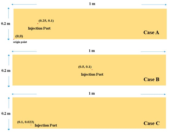
Figure 1. Selected cases with different injection port positions: case A (top picture), case B (middle picture) and case C (bottom picture). The coordinates of the points are given in meters with respect to the origin point.

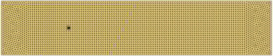
Figure 2. Finite element mesh used for case A in Figure 1.

The resulting fill times and injectability numbers for each inlet position and injection condition are reported in Table 2. It is noticeable that the injectability number is basically independent of the injection condition (slight differences can be ascribed to round-off and numerical errors in simulations and calculations) but varies with the position of the gate and thus, the filling pattern. The lowest injectability number was found in the case of the inlet placed at the center point of the rectangle (case B). In this case, the injectability number is also lower than the obtained value in Table 1. This suggests that a central inlet corresponds to a more favorable configuration for filling the cavity compared to the case of unidirectional line injection. Using Equation (3), the equivalent mold length for the central inlet case is calculated as approximately 0.73 m, which is smaller than the actual length L. Note that also the inlet point in case A returns a lower injectability number than the one for a unidirectional injection and the equivalent length (about 0.92 m) is lower than L as well. On the contrary, in case C, the resulting injectability number is greater than In for a unidirectional injection and the equivalent length (about 1.08 m) is greater than the actual length L.

Table 2. Fill times and injectability numbers for injection cases through a point inlet.

Case	Test	Injection Condition	Fill Time [s]	Injectability Number/109
A	1	Constant injection pressure	421	0.842
	2	Constant flow rate	150	0.838
	3	Time-dependent injection pressure	460	0.840
	4	Time-dependent flow rate	190	0.838
B	1	Constant injection pressure	265	0.531
	2	Constant flow rate	150	0.528
	3	Time-dependent injection pressure	305	0.531
	4	Time-dependent flow rate	190	0.528
C	1	Constant injection pressure	580	1.16
	2	Constant flow rate	150	1.16
	3	Time-dependent injection pressure	620	1.16
	4	Time-dependent flow rate	190	1.16

2.3. Injection through a C-Shaped Inlet

Figure 3 illustrates the injection port geometries for the two investigated cases of injection through a C-shaped inlet. The results are reported in Table 3 and show once again the substantial invariance of the injectability number with respect to the injection conditions. Moreover, taking into account the unidirectional injection case of Section 2.1, it could be concluded that the value of the injectability number decreases with increasing length of the inlet segments, which, in fact, facilitates mold filling.

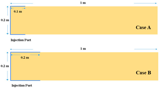
Figure 3. Selected cases of injection through a C-shaped inlet: case A (top picture) and case B (bottom picture).

Table 3. Fill times and injectability numbers for injection cases through a C-shaped inlet.

Case	Test	Injection Condition	Fill Time [s]	Injectability Number/109
A	1	Constant injection pressure	446	0.892
	2	Constant flow rate	151	0.893
	3	Time-dependent injection pressure	486	0.892
	4	Time-dependent flow rate	191	0.893
B	1	Constant injection pressure	360	0.721
	2	Constant flow rate	152	0.722
	3	Time-dependent injection pressure	401	0.722
	4	Time-dependent flow rate	192	0.723

Here, it is worth giving insight into how the C-shaped inlets are modeled in the PAM-RTM software. In order to simulate the reality of the gates accurately, the C-shaped inlets are introduced as 5 mm-wide and highly permeable segments (K_inlet = 2.5 × 10⁻⁶ m² >> K_preform = 2.5 × 10⁻¹⁰ m²) with the injection boundary conditions set on the middle point of the short side (Figure 4). At this middle point, P_inj(t) is computed and used for the calculation of the injectability number through Equation (1). Note that a possible different approach to define the gate in the software would consist in setting the injection boundary conditions directly on the edge elements of the preform. However, the latter approach is virtually equivalent to setting multiple inlet points and returns different results in the case of a flow rate controlled injection because the pressure P_inj(t) is not spatially constant along the inlet edges at any given time t. Figure 5 illustrates that some differences in the flow front shapes are obtained depending on the way the inlet gate is modeled, resulting in different injectability numbers. As shown in Part I, the invariance of the injectability number is preserved when the filling follows the same flow pattern regardless of the injection conditions. Figure 5 also compares the results in the case where the liquid is injected from a corner of the high permeable segments instead of the middle point of the short side: thanks to the fast flow in the inlet channels, the flow fronts show negligible differences and the injectability numbers are nearly the same.

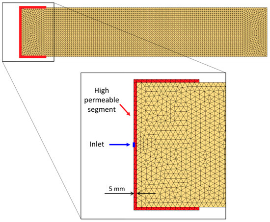
Figure 4. Design of C-shaped inlet used for simulating case A in Figure 3.

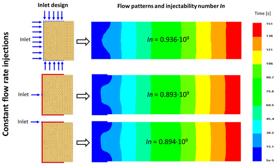
Figure 5. Comparison of flow patterns and injectability numbers obtained in constant flow rate injections for different designs of the C-shaped inlet.

2.4. Peripheral Injection

In the peripheral injection, the inlet gate is set along the whole perimeter of the laminate (Figure 6). This can be seen as the limit case of the C-shaped inlet configuration of Section 2.3. As before, the gate is modeled in the software using high permeable segments (K_inlet >> K_preform) around the preform edges and the resin is injected from the middle point of the short side on the left.

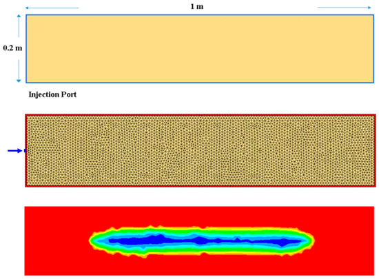
Figure 6. Peripheral injection case: geometry (top picture), mesh with surrounding high permeable segments (middle picture) and filling pattern with air entrapment (bottom picture).

The results, summarized in Table 4, show that such a configuration returns the lowest injectability number compared to all previously analyzed cases. However, as displayed by Figure 6, the peripheral injection strategy leads to air entrapment in the middle of the laminate, which must be avoided for optimal cavity filling. The process engineers should design the mold positioning the outlet vent at last place of cavity reached by the resin at the end of the filling.

Table 4. Fill times and injectability numbers for peripheral injections.

Test	Injection Condition	Fill Time [s]	Injectability Number/109
1	Constant injection pressure	6.23	0.0125
2	Constant flow rate	158	0.0125
3	Time-dependent injection pressure	43.2	0.0125
4	Time-dependent flow rate	198	0.0125

3. Vehicle Hood

This section examines the molding of a composite vehicle hood in order to apply the concept of the injectability number to a part of higher complexity and industrial interest than a rectangular laminate. Two hood geometries are analyzed. In the first case, the analysis aims at verifying that the injectability number does not change if the resin viscosity varies over time. The second case, instead, compares the fabrication methods of RTM and C-RTM by the difference in injectability numbers.

3.1. Injection with Constant and Variable Viscosity

Figure 7 illustrates the investigated cavity geometry and the simulated filling, which reproduces an injection through a central inlet gate by RTM. Thin shell elements are used in the simulations, which, unlike the other tests presented in this article, are carried out using the software COMSOL Multiphysics [9,10,11]. A preform with porosity of 0.5 and anisotropic permeability is considered: the principal permeability values are K₁ = 5 × 10⁻¹⁰ m² and K₂ = 2.5 × 10⁻¹⁰ m², aligned along the x and y axes respectively. Two inputs for the viscosity are examined: a constant viscosity of 0.1 Pa·s and a time-dependent viscosity, as displayed in Figure 8. The input of a variable viscosity is intended to simulate the effects of resin curing and/or temperature changes during the injection. It is worth pointing out that the resin viscosity is assumed to vary uniformly in every place inside the mold cavity, as if temperature or degree of curing change simultaneously in the volume of injected resin (namely, they change in time, but are spatially constant). Two injection conditions are also analyzed: a constant injection pressure of 3 bar and a constant flow rate of 20 cm³/s. Table 5 reports the results for each simulated case. As expected, although the filling time changes depending on the injection condition and viscosity input, the injectability number remains invariant.

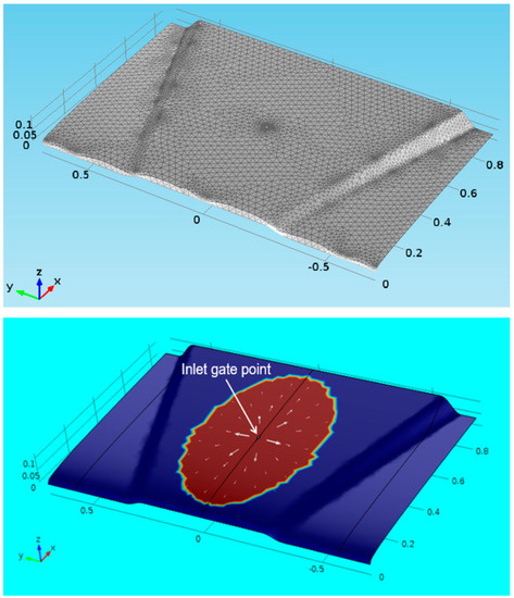
Figure 7. First geometry (top picture) and injection simulation (bottom picture) of composite vehicle hood (distances are given in meters).

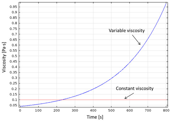
Figure 8. Viscosity curves for the filling simulations of the first hood geometry.

Table 5. Fill times and injectability numbers for filling cases of the first hood geometry.

Viscosity	Test	Injection Condition	Fill Time [s]	Injectability Number/109
Constant	1	Constant injection pressure	450	1.35
	2	Constant flow rate	307	1.35
Variable	1	Constant injection pressure	319	1.35
	2	Constant flow rate	307	1.35

3.2. Comparison of RTM and C-RTM

Figure 9 displays the second investigated example of vehicle hood geometry. This geometry is used as a reference to compare standard RTM and Compression-RTM. For both processes, the resin viscosity is set to 0.1 Pa·s and two injection conditions are considered: constant injection pressure of 4 bar and constant flow rate of 20 cm³/s. In the case of standard RTM simulations, the fiber volume content (v_f = 1 − φ) is fixed to 50% and the chosen permeability values are K₁ = K₂ = 10⁻⁹ m² (through-thickness flow is not simulated). For the C-RTM simulations, the mold cavity has an initial maximum thickness of 9.48 mm (with a maximum mold opening of 5 mm). After enough resin volume is injected [12], the inlet gate is closed and the preform is compressed to reach the final thickness of 4.48 mm with a compression speed of 6 mm/min. The fiber volume content in the cavity increases from about 24% to 50%, and the permeability values vary along with the fiber volume content, as shown in Figure 10 and Figure 11. At the final fiber volume content of 50%, the same as in the RTM simulations, the in-plane and through-thickness permeability values are K₁ = K₂ = 10⁻⁹ m² and K₃ = 0.5 × 10⁻¹¹ m² respectively.

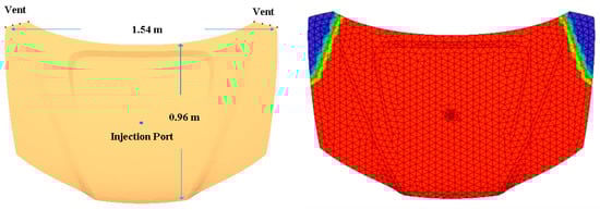
Figure 9. Second geometry (left) and injection simulation (right) of composite vehicle hood.

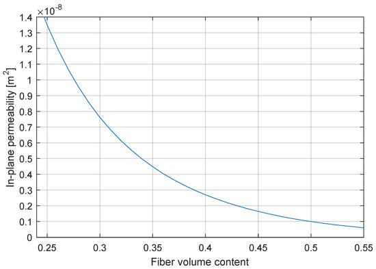
Figure 10. In-plane permeability (K₁, K₂) curve for the C-RTM process simulations for the second hood geometry.

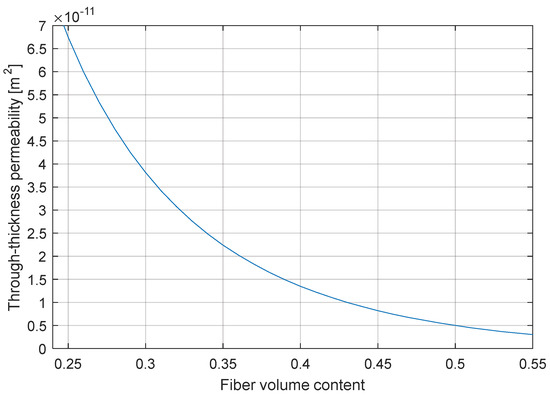
Figure 11. Through-thickness permeability (K₃) curve for the C-RTM process simulations for the second hood geometry.

Table 6 summarizes the resulting filling times and injectability numbers. It is observable that the injectability number of the C-RTM process is an order of magnitude lower than the one obtained for the standard RTM process. This suggests that the through-thickness flow occurring in C-RTM contributes to facilitate the cavity filling, even if the through-thickness permeability is much lower than the in-plane permeability. Table 7 shows the results obtained simulating the C-RTM process with different compression speeds, namely the speeds set to close the mold cavity to the final thickness. Obviously, lower speeds increase the filling times, but apparently, they have a minimal influence on the injectability number (within the considered range of speeds).

Table 6. Fill times and injectability numbers for filling cases of the second hood geometry.

Process	Test	Injection Condition	Fill Time [s]	Injectability Number/109
RTM	1	Constant injection pressure	144	0.573
	2	Constant flow rate	106	0.570
C-RTM	1	Constant injection pressure	53.4	0.0624
	2	Constant flow rate	208	0.0623

Table 7. Fill times and injectability numbers for C-RTM simulations of the second hood geometry at different compaction speeds.

Process	Injection Condition	Speed [mm/min]	Fill Time [s]	Injectability Number/109
C-RTM	Constant injection pressure	6	53.4	0.0624
		4	78.4	0.0625
		2	153	0.0626
		1	303	0.0629

4. Composite Reservoir

In this section, the injectability number is used to compare the standard process of RTM and the VARI, in which the mold is closed by a flexible plastic bag and the resin is infused into the fibrous preform by creating vacuum. A part geometry that resembles the shell of a reservoir, as shown by Figure 12, is taken as a reference example for this comparison. The resin inlet corresponds to the central circle of the shell (its diameter is 10 cm). The outlets correspond to the four corners in the case of RTM and to the whole rectangular perimeter for the VARI. Therefore, in the latter process, there is a partial resin outflow before the preform is fully impregnated. The fill time is computed as soon the filling is completed in all corners (post-filling time must not be considered for the calculation of the injectability number).

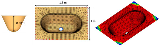
Figure 12. Geometry, mesh and injection simulation of composite reservoir.

Comparison of RTM and VARI

In order to equally compare RTM and VARI processes, the simulations are carried out considering a constant injection pressure of 1 bar. The resin viscosity is taken constant and equal to 0.1 Pa·s and the permeability curves shown in Figure 10 and Figure 11 are used. For the RTM simulation, the fiber volume content is fixed to 50% and the thickness to 3 mm. For the VARI, instead, the fiber volume content (as well as the thickness) is a function of the pressure [12] and the compaction curve shown in Figure 13 is considered for the simulation.

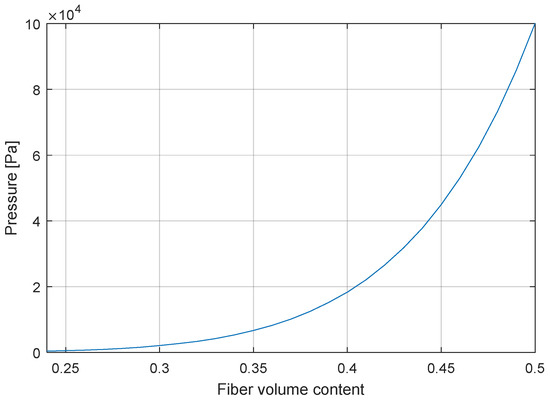
Figure 13. Compaction curve used in VARI simulation.

The results are reported in Table 8. As can be noticed, the VARI process gives a lower injectability number than the standard RTM.

Table 8. Fill times and injectability numbers for filling cases of the reservoir geometry.

Process	Injection Condition	Fill Time [s]	Injectability Number/109
RTM	Constant injection pressure	406	0.406
VARI	Constant injection pressure	317	0.317

5. Aircraft Fuselage Section

The final application example for the injectability number corresponds to the molding of a complex ribbed part, representing a sandwich composite section of an aircraft fuselage. The part geometry is detailed in Figure 14 and Figure 15; it is made up of a curved thick laminate with a hole in the middle for a window and with attached formers and stringers. As depicted by Figure 14, the curved laminate, the two formers and the stringers constitute three distinct preform zones, whose principal permeability values are listed in Table 9.

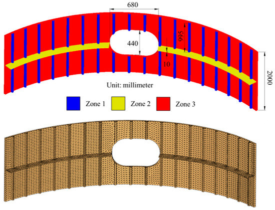
Figure 14. Fuselage section geometry and mesh.

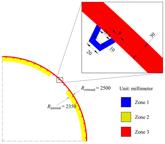
Figure 15. Details of the fuselage section geometry.

Table 9. Preform zones and corresponding principal permeability for the fuselage section (permeability K₁ and K₂ are always the in-plane values, while K₃ the through-thickness value).

Preform Zone	K1 [m2]	K2 [m2]	K3 [m2]
Zone 1	10−14	10−14	10−14
Zone 2	10−12	10−12	10−12
Zone 3	10−10	10−10	5 × 10−11

Four different RTM injection configurations were simulated:

• Case A—Injection from the central hole (Figure 16)
  

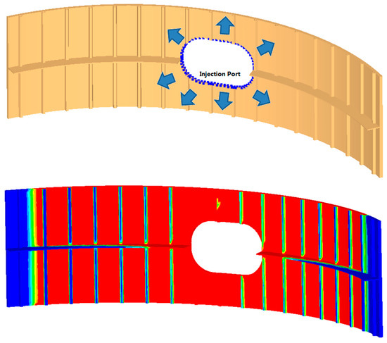  Figure 16. Injection case A for the fuselage section.
• Case B—Injection from the long sides (Figure 17)
  

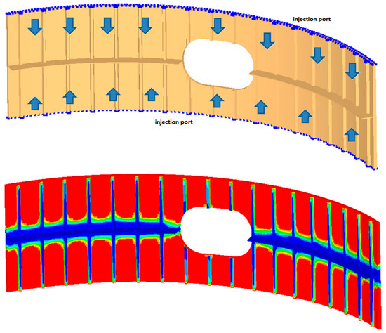  Figure 17. Injection case B for the fuselage section.
• Case C—Injection from the short sides (Figure 18)
  

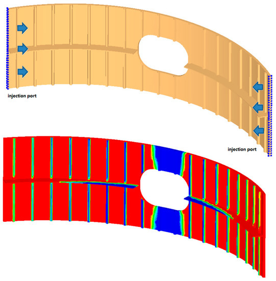  Figure 18. Injection case C for the fuselage section.
• Case D—Through-thickness injection from the back side of the curved laminate (Figure 19)
  

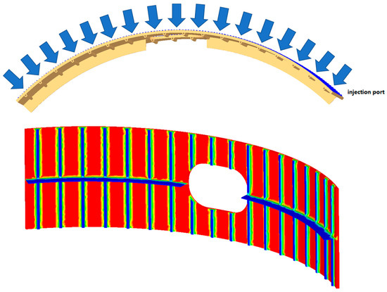  Figure 19. Injection case D for the fuselage section.

All simulations were carried out using the same viscosity of 0.1 Pa·s, a fiber volume content of 50% and two different conditions for resin input: a constant injection pressure of 4 bar and a constant flow rate of 20 cm³/s. The results, summarized in Table 10, show that the lowest injectability number and filling times are given by the injection strategy corresponding to the case C. For each case, the differences in the injectability numbers between pressure and flow rate controlled injections are minimal (less than 1%) and could be attributed to numerical errors in computer simulations and in the integration to calculate In.

Table 10. Fill times and injectability numbers for filling cases of the fuselage section.

Case	Test	Injection Condition	Fill Time [s]	Injectability Number/1011
A	1	Constant injection pressure	6510	0.260
	2	Constant flow rate	3010	0.262
B	1	Constant injection pressure	6445	0.260
	2	Constant flow rate	3010	0.261
C	1	Constant injection pressure	5010	0.203
	2	Constant flow rate	3010	0.204
D	1	Constant injection pressure	5340	0.214
	2	Constant flow rate	3010	0.215

6. Conclusions

The dimensionless parameter called the injectability number enables a quantitative evaluation of molding complexity for liquid injections through porous media. This number is invariant with respect to the inlet conditions. Injections at both constant and time-varying inlet pressure or flow rate provide the same injectability number for identical mold configuration and preform characteristics. The invariance property was mathematically demonstrated in Part I and verified in Part II by means of computer simulations of mold cavity filling. The investigation focused initially on different injection strategies to fill a plain rectangular cavity. In addition to the verification of the invariance of the injectability number, the results show that lower values of this number are associated to more efficient filling strategies according to common practice in LCM.

The analysis was then extended to a series of composite molding cases of growing complexity: two geometric models of a vehicle hood, a perforated reservoir shell and an aircraft fuselage section. In addition to verifying again the invariance of the injectability number (negligible discrepancies of less than 1% fell within the numerical error range), the investigated cases were used to compare different LCM processes, such as RTM, C-RTM and VARI. Lower injectability numbers could be obtained by C-RTM and VARI processes in comparison to standard RTM, suggesting that the latter would lead to more difficult resin injections in the analyzed examples. This result confirms the practical experience of composite manufacturers, who developed alternatives to traditional RTM to overcome process limitations and to increase efficiency.

In summary, the dimensionless injectability number turns out to be a useful tool to measure the LCM complexity of a composite part and to rate different cavity filling strategies. It can help not only to optimize the molding configuration, but also to select a suitable LCM process. Future investigations could focus on setting up experimental procedures to evaluate practical ranges of values for the injectability number. It would also be interesting to extend the scope of application of this new concept to injections with temperature gradients and to include the optimization of the resin cure.

References

- Parnas, R.S. Liquid Composite Molding; Carl Hanser Verlag GmbH: Munich, Germany, 2000. [Google Scholar]
- Strong, A.B. Fundamentals of Composites Manufacturing: Materials, Methods and Applications; Society of Manufacturing Engineers: Southfield, MI, USA, 2008. [Google Scholar]
- Advani, S.G.; Hsiao, K.-T. Manufacturing Techniques for Polymer Matrix Composites (PMCs); Woodhead Publishing Limited: Cambridge, UK, 2012. [Google Scholar]
- Ermanni, P.; Di Fratta, C.; Trochu, F. Molding: Liquid Composite Molding (LCM). In Wiley Encyclopedia of Composites; Nicolais, L., Borzacchiello, A., Eds.; John Wiley & Sons, Inc.: Hoboken, NJ, USA, 2012; pp. 1884–1894. [Google Scholar]
- Controlled Vacuum Infusion (CVI)—Product and Services—Polyworx. Available online: http://www.polyworx.com/pwx/cvi/ (accessed on 28 August 2019).
- Simacek, P.; Advani, S.G. Desirable features in mold filling simulations for liquid composite molding processes. Polym. Compos. 2004, 25, 355–367. [Google Scholar] [CrossRef]
- Arbter, R. Contribution to Robust Resin Transfer Molding. Ph.D. Thesis, ETH Zurich, Zurich, Switzerland, 2008. [Google Scholar]
- PAM-RTM—Composites Molding Simulation Software. Available online: https://www.esi-group.com/software-solutions/virtual-manufacturing/composites/pam-composites/pam-rtm-composites-molding-simulation-software (accessed on 28 August 2019).
- Di Fratta, C.; Klunker, F.; Ermanni, P. A methodology for flow-front estimation in LCM processes based on pressure sensors. Compos. Part A 2013, 47, 1–11. [Google Scholar] [CrossRef]
- Di Fratta, C.; Koutsoukis, G.; Klunker, F.; Ermanni, P. Fast method to monitor the flow front and control injection parameters in resin transfer molding using pressure sensors. J. Compos. Mater. 2016, 50, 2941–2957. [Google Scholar] [CrossRef]
- Di Fratta, C. Combined Experimental–Numerical Methods to Monitor Liquid Composite Molding and Characterize Textile Permeability. Ph.D. Thesis, ETH Zurich, Zurich, Switzerland, 2015. [Google Scholar]
- PAM-RTM 2014 User’s Guide & Tutorials; ESI Group: Paris, France, 2014.
© 2020 by the authors. Licensee MDPI, Basel, Switzerland. This article is an open access article distributed under the terms and conditions of the Creative Commons Attribution (CC BY) license (http://creativecommons.org/licenses/by/4.0/).