Improving Prediction Accuracy and Robustness in Injection Mechanism Based on Simplified Pareto and Updated Training Set Hybrid Metamodel

Abstract

In squeeze casting, the injection parameters including fit clearance, speed, temperature, and their uncertainties significantly impact the forming quality. Robust optimization can improve the design reliability and reduce the influence of uncertainty while using a suitable metamodel is beneficial for prediction accuracy and efficiency. This paper proposes a robust optimization method based on a hybrid metamodel with Simplified Pareto and Updated Training Set (SPUTS) to improve the prediction accuracy along the Pareto front and in the whole design space. After the first round of robust optimization based on a general metamodel, the training set is updated by simplifying the Pareto solution set. A finite element simulation is performed to construct a high-precision metamodel that combines the kriging and radial basis function (RBF) models to run a new robust optimization. The proposed method was validated by application to the robust optimization of an injection mechanism with a large inner diameter. The results indicated that the SPUTS hybrid metamodel greatly reduced the prediction errors in the test set. The optimized design showed better reliability and robustness and had a greater clearance ratio than the initial design.

1. Introduction

In contrast to deterministic optimization, robust optimization considers the uncertainty of parameters, which can reduce the fluctuation of the target response and obtain a more robust design [1]. Manufacturing process parameters are usually characterized by large uncertainties that are difficult to control accurately but require high reliability. Ignoring uncertainty significantly affects the system’s reliability. Robust optimization takes the statistical characteristics of the target response such as the mean and variance as optimization objectives [2,3]. Therefore, even if the parameters fluctuate, the response can be improved, which is more suitable for process parameter optimization. Six Sigma (6σ) uses sigma (σ) levels to characterize the reliability of a design, which can be combined with robust optimization [4,5]. A reliable and robust design can be obtained by 6σ robust optimization of process parameters.

Robust optimization usually uses the Monte Carlo method to calculate the response of a large number of sample points to obtain the statistical characteristics of the target response. Numerical simulations are commonly used to calculate the target response in engineering problems. However, numerical simulations require significant computational resources and time, so metamodels are increasingly being used for robust optimization because of their calculation efficiency. Liu et al. combined a kriging model and the Taguchi method for robust optimization of vehicle stability [6]. Wang et al. built a radial basis function (RBF) model and used the Taguchi method to obtain the combination of parameters that resulted in the most robust suspension to optimize the vertical driving stability of high-speed rail vehicles [7]. Du et al. used a Kriging model with a local surrogate strategy for a high-speed permanent magnet synchronous machine, shortening the optimization time and greatly reducing the prediction error [8]. Xiong et al. applied robust optimization to the aerodynamic performance of a low-resistance airfoil and established a two-stage kriging model to consider the mean and variance [9]. Xue et al. combined reliability-based robust optimization design and surrogate model in aerospace thin-walled components to improve robustness and versatile performance [10].

Metamodels are used to represent the relationship between inputs and outputs, and their accuracy determines the prediction accuracy of the robust optimization. Common metamodels include the response surface model [11,12], kriging model [13,14], and RBF model [15,16,17], all of which have been applied to various engineering modeling problems. Some comparative analyses have facilitated the rational selection of various metamodels. Jin et al. compared the optimization results of three metamodels and found that the response surface model had a large error when applied to high-order nonlinear behavior [18]. In addition, the coefficients of the high-order polynomial regression were difficult to solve, and the accuracy could not be guaranteed. In contrast, the kriging and RBF models accurately approximated various low- and high-order nonlinear behaviors, but the RBF model was more irregular and was prone to overfitting, which easily led to an increase in local errors. Yondo et al. compared the kriging and response surface models and found that, although the high-order response surface is applicable to highly nonlinear problems, it needs a large training set and thus has an unstable performance [19]. In contrast, they found that the kriging model obtained better results from noisy data. In general, the kriging and RBF models construct more accurate interpolation models for various problems. The response surface model can only approximate some simple processes and requires large and high-quality training sets.

However, although the kriging and RBF models are suitable for various problems, their application to realizing high-precision robust optimization for complex problems considering uncertainties is still a challenge. Robust optimization requires high accuracy along the Pareto front to obtain more accurate statistical characteristics and robust solutions. Moreover, the metamodel needs to represent the whole process so that the Pareto front accurately reflects the whole design space.

Some approaches to improving the prediction accuracy of a metamodel are to reduce the modeling space and add sample points in the region of interest. Adding sample points can improve the accuracy without reducing the search area. Liu et al. optimized a permanent magnet linear synchronous motor using a Kriging model, boosting prediction accuracy from 76% to 99.7% via expected improvement-based sampling [20]. However, this criterion depends on Kriging’s predictive variance and is not transferable to other surrogates. Xie et al. combined the extended finite element method with a Kriging surrogate model and Latin hypercube sampling for crack identification, significantly improving prediction accuracy [21]. Li et al. introduced a high-fidelity surrogate modeling approach based on Kriging and a parallel multipoint expected improvement infill strategy, which attains high predictive accuracy for both low-dimensional and high-dimensional complex problems [22]. Gu et al. introduced an adaptive point selection approach for structural reliability analysis, combining a Kriging surrogate model and a learning function to achieve more accurate reliability predictions [23]. Chen et al. proposed a new infill point selection strategy that combines RBF neural networks with a genetic algorithm, achieving faster convergence and better performance than traditional methods [24]. Wang et al. utilized K-means clustering on a Pareto front and obtained three representative points for analysis with a reduced workload [25]. Vural et al. employed a fuzzy c-means clustering algorithm to process a Pareto front and obtain a compromise solution [26]. Zhang and Xu conducted the Taguchi method to obtain an initial optimal solution and then reduced the design space and built a metamodel with higher precision [27]. Their method is suitable for optimization problems with a large design space. However, reducing the design space limits the search area, which decreases the diversity of the Pareto solution set in the case of multi-objective optimization. Fang and Tang proposed a metrics planning-based Pareto equilibrium algorithm to select a single solution from a high-dimensional Pareto set; however, its sensitivity to the reference point, static weights, and assumption of a unique optimum limit its use in uncertain, complex engineering problems [28].

Hybrid metamodels are an effective approach to improving the prediction accuracy for the whole design space. Lee et al. built a hybrid metamodel by combining the kriging and response surface models, which they applied to optimizing the design of a double bar, spring, and drive shaft [29]. Their optimal solution was closer to the exact solution than the optimal solutions of the separate sub-models. Long et al. proposed a hybrid metamodel with adaptive sampling for the lightweight optimization design of car seats [30]. Of the nine models considered, they selected three to construct the hybrid metamodel and obtained a more accurate optimal solution. Lv et al. developed a hybrid surrogate mode using the attention mechanism to automatically decide the weights of the sub models according to the working conditions to ensure its approximation ability under all working conditions, which featured lower error and higher performance [31].

Squeeze-casting is a typical complex engineering problem that requires consideration of uncertainty [32,33] It is widely used in machinery, automobile, household appliances, aerospace, and other industries [34]. The injection mechanism is a core component of the squeeze-casting machine. During the working process, deformation of the injection mechanism can change the clearance between the shot sleeve and punch, which affects the overall machine performance. In our previous work [35,36,37], we proposed a friction model for an injection mechanism with a small inner diameter to improve the simulation accuracy and established a kriging model to optimize the injection parameters. However, the deformation of an injection mechanism with a large inner diameter is more complicated and has greater uncertainty. Thus, the kriging model needs to be replaced with a high-precision metamodel to achieve robust optimization and reduce the influence of parameter uncertainty. Existing Pareto-clustering methods often ignore uncertainty in objective predictions, leading to overconfident front representations. Most adaptive sampling strategies focus on convergence or diversity but lack explicit robustness-aware criteria that account for both mean and variance under input perturbations. Few methods integrate Pareto simplification and uncertainty-aware retraining in a unified loop, which is a core feature of SPUTS.

We propose a robust optimization method based on a hybrid Kriging-RBF (K-R) metamodel with Simplified Pareto and Updated Training Set (SPUTS), aiming to improve prediction accuracy along the Pareto front and across the design space. The Pareto set is simplified by removing points close to previous training data, followed by clustering. The training set is then updated using a finite element (FE) simulation of the simplified Pareto solutions. The hybrid K-R model enhances global prediction accuracy, and orthogonal experiments are used to optimize process parameter weights. The proposed method is applied to the robust optimization of large inner diameter injection mechanisms, which are key components in precision manufacturing and effectively balance the clearance between the injection sleeve and the punch. By combining simulation-driven design with efficient proxy modeling, the proposed method can achieve reliable, economical and high-quality production in the real process.

2. Methodology

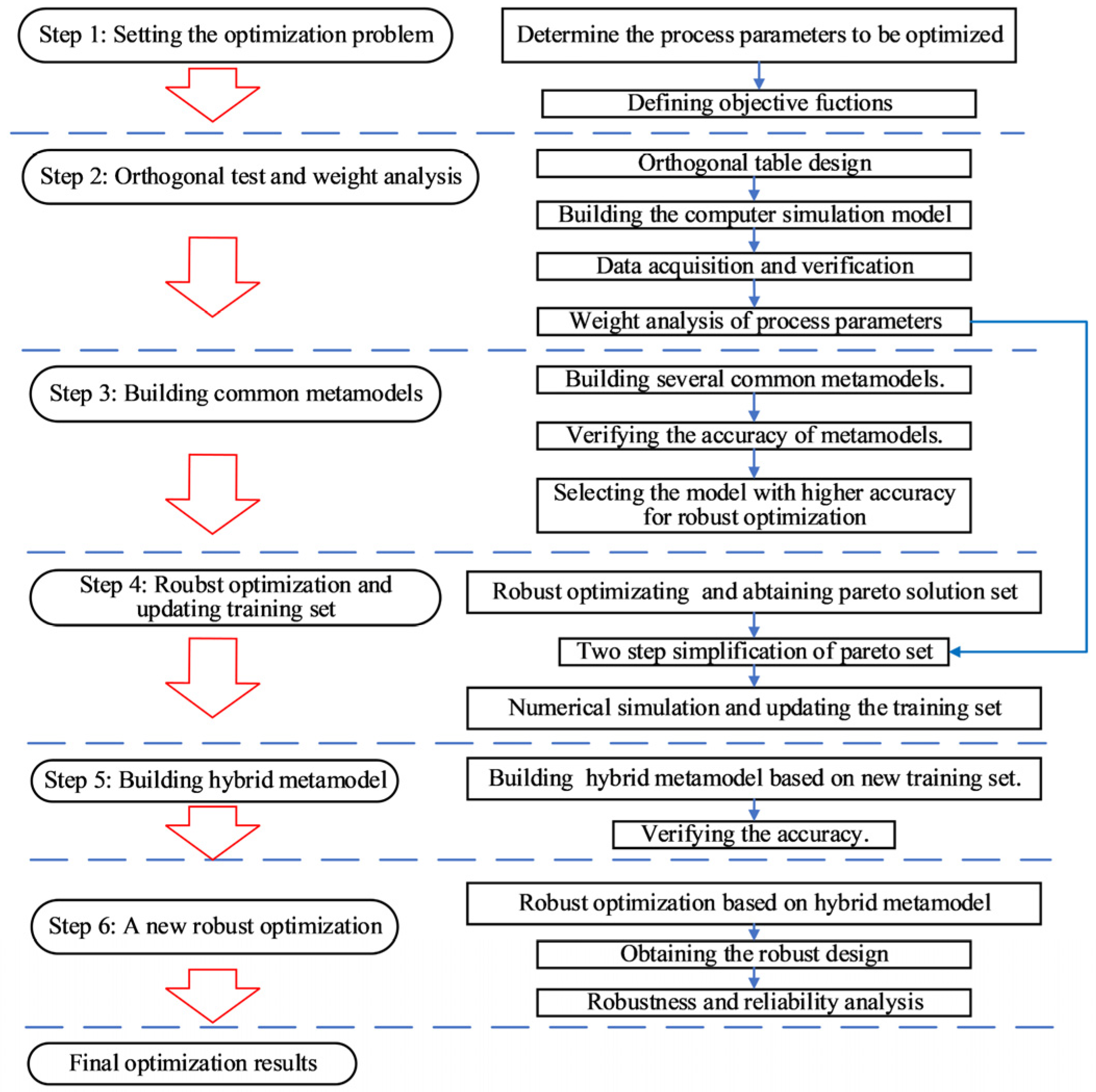
The proposed robust optimization method uses a hybrid K-R metamodel with SPUTS for process parameter optimization to consider both local and global accuracy. Figure 1 shows the flowchart of the proposed method, which includes orthogonal experiments for parameter weight analysis, an initial robust optimization, a two-step simplification of the Pareto solution set and update of the training set, construction of the hybrid metamodel, and a new round of robust optimization.

Figure 1. Flowchart of the proposed method.

2.1. Parameter Weight Analysis and SPUTS

Although Latin hypercube sampling greatly simplifies the number of experiments to obtain data, it is not conducive to parameter analysis. In this study, orthogonal experiments were performed to obtain a small number of uniformly distributed sample points that represent the whole design space, which can then be used to analyze the influence of parameters. These sample points can be used as training sets for subsequent modeling. They are tested in the orthogonal experiment L_n(t^c), where n is the total number of tests, t is the number of levels, and c is the number of parameters. The dispersion degree of the response mean in orthogonal experiments is employed for quantitative analysis of the influence of parameters. A greater dispersion degree indicates that a parameter has a greater influence on the response; in other words, a change in the parameter causes a drastic change in the response. The dispersion degree is expressed by the standard deviation of the response mean to different levels of the influencing parameter:

$$std(F_i)=\sqrt{{\displaystyle \sum _{j=1}^t{(Z_{ij}-\mu )}^2/t}}$$

(1)

where std(F_i) is the standard deviation of the response mean to the i-th parameter and Z_ij is the response mean to the i-th parameter at the j-th level. t is the number of levels, and μ is the mean of all responses, so each parameter has the same μ.

Parameters can be weighted to quantitatively characterize their influence. A parameter with a higher dispersion degree is given a greater weight. The parameter weights can be calculated for Equation (2).

$${\omega }_i={\displaystyle \frac{std(F_i)}{{\displaystyle \sum _{k=1}^{c}std(F_k)}}}{\displaystyle \sum _{i=1}^c{\omega }_i}=1$$

(2)

where ω_i is the weight of the i-th parameter and ${\displaystyle \sum _{k=1}^{c}std(F_k)}$ is the sum of the standard deviations of the response means of all parameters.

Usually, a certain scale of Pareto solution set is obtained after robust optimization. By numerical calculating the responses of these Pareto points and adding them as new sample points to the training set, the accuracy of the model can be improved. To improve the local accuracy around Pareto solutions and avoid excessive FE simulation, some Pareto solutions representing the whole solution set were simplified and retained for building a metamodel. The update process has the following steps: simplify the Pareto solution set, simulate the simplified Pareto solution set, update the training set, and construct the hybrid K-R metamodel for robust optimization.

The Pareto solution set is simplified in two steps:

(1)

Pareto solutions close to the sample points in the training set of the previous step are deleted. The shortest spatial distance is used to determine the closeness between a Pareto solution and sample point and is calculated for Equation (3).

$$\min dis(x_i,X)=\underset{j\widehat{I}\left(1,2\dots \dots ,n\right)}{\min }dis(x_i,x_j)$$

(3)

where x_i is the i-th sample point in the Pareto solution set, X is the training set of the previous step with n sample points, x_j is the j-th sample point in X, and dis(x_i, x_j) is the spatial distance between x_i and x_j. Then, $\min dis(x_i,X)$ is the shortest spatial distance between x_i and X.

(2)

The spatial distance is used as the evaluation criterion for K-means clustering of the Pareto solutions to obtain representative and evenly distributed sample points. The obtained cluster centroids are numerically simulated and are used to update the training set. The K-means clustering includes the following steps: initialize k points in the design space as the centroid of the initial class, assign each solution to the nearest centroid in the space and divide them into k classes, and recalculate the centroids of the k classes. The solution assignment and centroid recalculation are then repeated until the centroids converge or no longer move.

The spatial distance is used in both steps of the Pareto solution set simplification. The spatial distance is commonly represented by the Euclidean distance, which assumes that all dimensions are equal. However, the influence of each parameter on the target response of the optimization process is often different. Thus, the parameter weight analysis in Section 2.1 can be used to develop a more suitable spatial distance for Equation (4).

$$dis(x_i,x_j)=\sqrt{{\displaystyle \sum _{k=1}^c({\omega }_k(x_i^k-x_j^k))}}$$

(4)

where $x_i^k$ and $x_j^k$ are the k-th parameter values of sample points x_i and x_j, respectively, and ${\omega }_k$ is the weight indicating the influence of the k-th parameter.

Parameters with a greater influence on the target response are assigned a greater weight, which significantly affects the spatial distance and simplification results. Compared with low-weight parameters, high-weight parameters need to be closer to each other to be considered similar. This is also consistent with the fact that changes in high-weight parameters lead to greater changes in the target response.

2.2. Hybrid K-R Metamodel

The hybrid metamodel is an approximate model that combines sub-models to improve the prediction accuracy above that which can be obtained by the sub-models on their own. Equation (5) is the prediction formula.

$$y_{pred}={\displaystyle \sum _{i=1}^n{\delta }_i{y}_i}{\displaystyle \sum _{i=1}^n{\delta }_i}=1$$

(5)

where y_pred is the predicted value by the hybrid model, n is the number of sub-models, y_i is the predicted value by the i-th sub-model, and δ_i is the weight of the i-th sub-model. In this study, the kriging and RBF models were used, so n = 2. The weights of the sub-models directly affect the performance of the hybrid metamodel, and they can be optimized to reduce the prediction error. The root mean square error (RMSE) was used to measure the prediction error. Equation (6) is the objective function for minimizing the error.

$$\min \sqrt{{\displaystyle \frac{1}{m}}{\displaystyle \sum _{i=1}^m{\left(y_{pred}^i-y^i\right)}^2}}$$

(6)

where m is the number of samples, $y_{pred}^i$ is the predicted value by the hybrid model at the i-th sample point, and yⁱ is the actual value of the i-th sample point.

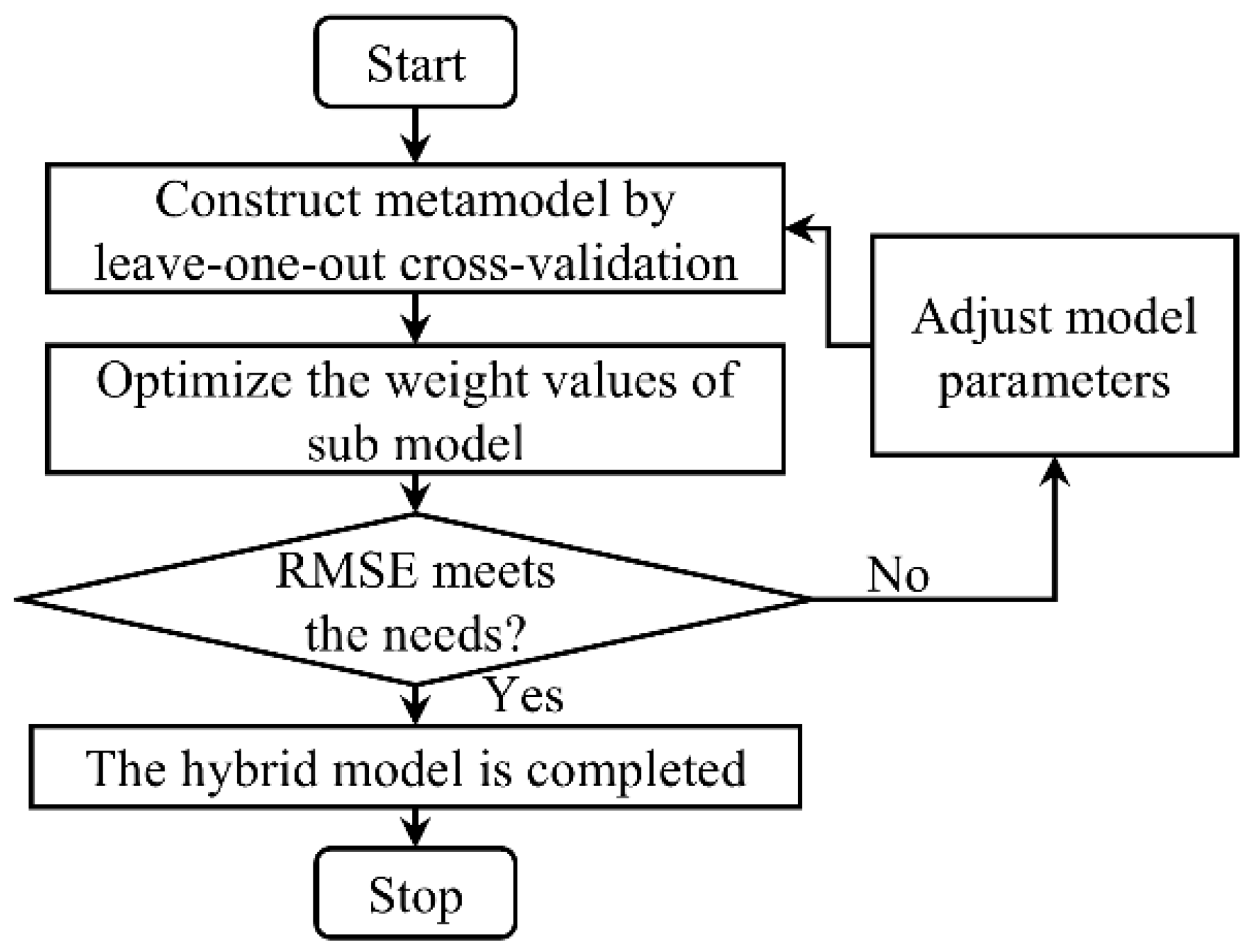
Figure 2 shows the construction process of the hybrid metamodel. The weights ${\delta }_1$ and ${\delta }_2=1-{\delta }_1$ were optimized by minimizing the leave-one-out cross-validation RMSE via an exhaustive grid search over ${\delta }_1\in [0,1]$ with a step size of 0.001. The hybrid prediction is a convex combination of the precomputed leave-one-out predictions from each sub-model. No explicit regularization was used; the convexity constraint and leave-one-out cross-validation inherently prevent overfitting. If the prediction error satisfies design requirements, the model construction is successful.

Figure 2. Construction of the hybrid metamodel.

2.3. 6σ Robust Optimization

In 6σ robust optimization, the σ level represents the design reliability, and the mean and variance of the response represent the robustness. The 6σ robust optimization model is as follows:

$$\begin{array}{l}\min : F_{obj}(u_y,{\sigma }_y)\\ s.t.\hspace{1em}{G}_i(u_y,{\sigma }_y)=u_y+n{\sigma }_y\le y_u, i=1,\dots ,q\\ \hspace{1em}\hspace{1em} G_j(u_y,{\sigma }_y)=u_y-n{\sigma }_y\ge y_l, j=1,\dots ,p\\ \hspace{1em}\hspace{1em} x+n{\sigma }_x\le x_u\\ \hspace{1em}\hspace{1em} x - n{\sigma }_x\ge x_l\end{array}$$

(7)

where the objective function F_obj contains q + p performance constraints: G_i, G_j; y_u and y_l are the highest and lowest required values of the optimization objective, respectively; x_u and x_l are the upper and lower limits, respectively, of the design parameter x; x and σ are the mean and standard deviation, respectively; and n is the σ level. A larger n indicates a more reliable design.

3. Validation and Application

The injection mechanism of a squeeze-casting machine was used for validation. Referring to the flowchart in Figure 1, the proposed method was applied to robust optimization of the process parameters. The effectiveness of the proposed method was evaluated by comparison with the results of the robust optimization method based on the ordinary kriging model.

3.1. Design Variables and Target Response

Four key parameters were selected as design variables: the pouring temperature (T_c), preheating temperature (T_m), injection velocity (V), and initial clearance (C₀). Table 1 presents their interval settings. The pouring temperature is determined by the material properties, the preheating temperature is set according to machine specifications, the injection velocity is calculated to ensure the entire process is completed within 88 s, and the initial clearance is assigned based on standard machine clearance.

Table 1. Interval settings of the selected design variables for the injection mechanism.

	Tc (°C)	Tm (°C)	V (mm/s)	C0 (mm)
Lower limit	700	100	40	0.05
Upper limit	760	400	76	0.17

The clearance rate, which is calculated from the deformations of the shot sleeve and punch, was used to characterize the stability of the injection process. The target response was set as the minimum clearance rate minCr:

$$\min Cr={\displaystyle \frac{\min (C_o-(D_p-D_s))}{C_o}}$$

(8)

where D_p and D_s are the radial deformations of nodes corresponding to the punch and shot sleeve, respectively, during the injection process. Because the shot sleeve generally deforms less than the punch, minCr ranges between 0 and 1. The injection process is more stable as minCr converges to 1.

3.2. Experiment and FE Simulation of Injection Mechanism

Figure 3a shows the experimental device. The main body of the injection mechanism comprised a shot sleeve, punch, base, and pushing rod. The shot sleeve had an inner diameter of 200 mm, wall thickness of 30 mm, height of 340 mm, and initial clearance of 0.15 mm. Measurement points for the temperature and displacement were set up by opening blind holes on the shot sleeve and punch, as shown in Figure 3b. The radial deformations of the shot sleeve and punch were measured by a dial gauge and strain gauge, respectively. Four deformation measurement points D1–D4 were arranged at equal distances of 30 mm apart on the shot sleeve, and one deformation measurement point D5 was on the punch. The temperature was measured by thermocouples at seven measurement points on the shot sleeve and one point on the punch. The punch had a vertical movement speed of 40 mm/s and stroke of 80 mm. The ambient temperature was 25 °C. The preheating temperature was about 220 °C.

Figure 3. Experimental device: (a) injection mechanism and (b) measurement points.

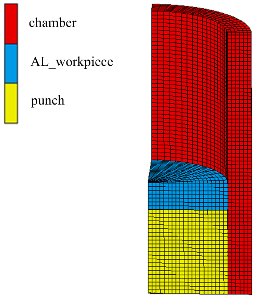
The friction model of the injection mechanism developed was used to establish a thermomechanical coupling transient FE model of the injection mechanism. Owing to the symmetry, only a quarter of the model was selected for numerical simulation. The finite element model was built in MSC Marc using 8-node hexahedral continuum elements (element type 7) with full integration. A global mesh size of 5 mm was employed. Figure 4 shows the 3D mesh of the model, which included 17,242 nodes and 13,960 hexahedral elements. Based on the physical assembly of the die casting system, the shot sleeve is rigidly mounted on the base and thus fully constrained in all translational directions. Accordingly, zero displacements were prescribed in the x, y, and z directions for the sleeve. The plunger is designed to move only axially (along the z-direction) within the sleeve. Therefore, its displacements in the x and y directions were constrained to zero, while motion in the z-direction was left free to simulate the injection process.

Figure 4. Finite element mesh of the experimental device.

The interface heat transfer coefficients were set to 500 W/(m²·K) between the shot sleeve and punch, 850 W/(m²·K) between the casting and shot sleeve, 450 W/(m²·K) between the casting and punch, and 10 W/(m²·K) between each component and the air [38]. The working environment temperature was 25 °C. Table 2 lists the material properties, which were set as consistent with the experimental device [39].

Table 2. Material properties of each component.

Material Properties	Punch	Shot Sleeve	Casting
Density (kg/m3)	7060	7800	2700
Young’s modulus (GPa)	169	210	-
Poisson’s ratio	0.257	0.3	-
Thermal conductivity (W/m·k)	24.5–32.2	25.0–34.2	60–160
Specific heat (J/kg·k)	560–856	460–520	963–1082
Linear expansion coefficient (10−5/K)	1.3	1.15	-

To ensure that the 5 mm mesh provides sufficient accuracy, a mesh independence study was conducted. Simulations were performed using progressively refined mesh sizes of 2.5 mm, 1.25 mm, and 1.0 mm. Taking the results from the 5 mm mesh as the reference, the maximum relative error in deformation at key measurement points was computed for each finer mesh. As summarized in Table 3, the maximum relative error remains below 1.5%, indicating that the 5 mm mesh yields accurate and reliable results. This coarser discretization significantly reduces the total number of elements and nodes, thereby improving computational efficiency without compromising solution fidelity.

Table 3. Comparison results of independence tests.

Mesh Size (mm)	Number of Elements	Maximum Relative Error (%)
5	13,960	0
2.5	111,680	1.21
1.25	893,440	1.45
1	1,745,000	1.53

The validation was focused on the radial deformation, so the experimental and simulation data on the deformation were compared to confirm the accuracy of the FE model. Figure 5 compares the radial deformations at five measurement points, where Sim stands for simulation results and Exp stands for experiment results. The overall trends of the experimental and simulated values were consistent. The maximum relative error was 16.89%, which occurred in the initial stage when deformation was small, and decreased to less than 10% in the rest of the process. Therefore, the FE model was confirmed as reliable and applicable to robust optimization.

Figure 5. Comparison of radial deformations in the experiment and simulation at selected measurement points: (a) D1–D3 and (b) D4 and D5.

4. Results and Discussions

4.1. Parameter Weight Analysis

The design variables and responses described in Section 3.1. And the FE model described in Section 3.2 were used to construct the orthogonal experiment L₉(3⁴) with four parameters and three levels in Table 4. A numerical simulation was carried out to construct the orthogonal dataset. The response means were used to calculate the weight of each parameter as per the procedure described in Section 2.1. The values are presented in Table 5 and show that C₀ has the largest weight value of 0.5897. T_m is assigned the second-largest weight (0.2682) among all factors. Nevertheless, the small weight values assigned to factors T_c and V imply that their contribution to the objective function is comparatively negligible. Owing to their significant impact on the target response, the initial clearance C₀ and preheating temperature T_m were included in the subsequent simplified process.

Table 4. L₉(3⁴) orthogonal table of different factors.

Tc	Tm	V	C0
1	1	1	1
1	2	2	2
1	3	3	3
2	1	2	3
2	2	3	1
2	3	1	2
3	1	3	2
3	2	1	3
3	3	2	1

Table 5. Response means and parameter weights.

Level	Tc	Tm	V	C0
1	0.8813	0.8526	0.8811	0.8102
2	0.8926	0.8905	0.9006	0.9128
3	0.8923	0.9196	0.8846	0.9433
Weight	0.0541	0.2682	0.0880	0.5897

The SPUTS hybrid surrogate model was developed using a total of 31 finite element simulations: 9 from an L₉(3⁴) orthogonal design for initial training, 18 for an independent Latin Hypercube Sampling-based test set, and 4 additional simulations of selected Pareto solutions for model refinement. The first robust optimization yielded 60 non-dominated solutions, which were reduced to 4 representative designs based on parameter influence weights. The updated training set (13 samples) was used to reconstruct the final high-fidelity SPUTS model.

4.2. Original Metamodel and First Robust Optimization

The above orthogonal dataset was used as the training set. The test set was obtained by random sampling and FE simulation in the intervals of the design variables. The kriging and RBF models were constructed based on the training set. The RMSE values of the two models when applied to the test set were 0.0271 and 0.0246, respectively. We constructed a hybrid metamodel using the approach outlined in Section 2.2 and derived the weight coefficients for the sub-models. The final optimized weights are ${\delta }_1=0.6010$ and ${\delta }_2=0.3990$.

The kriging model had a higher prediction accuracy, so it was selected as the metamodel for the first round of robust optimization. The parameters in Section 3.2 were taken as the initial design: a pouring temperature of 720 °C, preheating temperature of 220 °C, initial clearance of 0.15 mm, and injection velocity of 40 mm/s. The objectives of the robust optimization were the mean and variance of minCr. Because minCr converged to 1, a negative sign was added to minCr to conform to the optimization rules, the optimization model is given in Equation (9).

$$\min \left\{\begin{array}{l} u_{-\min C_r}\left(T_c,T_m,V,C_0\right)\\ {\sigma }_{-\min C_r}\left(T_c,T_m,V,C_0\right)\end{array}\right.s.t\left\{\begin{array}{l}700\le T_c\le 760\\ 100\le T_m\le 4000\\ 40\le V\le 76\\ 0.05\le C_{0c}\le 0.17\end{array}\right.$$

(9)

4.3. Robust Optimization of Design

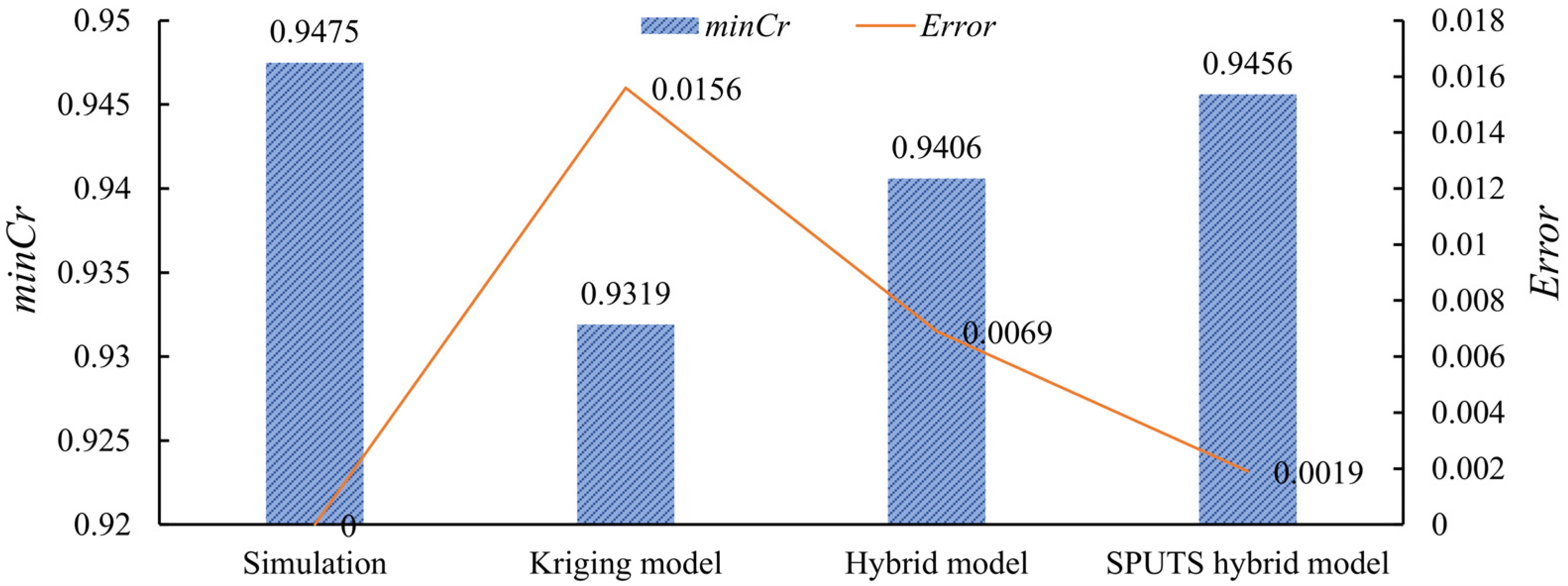
Figure 6 compares the simulation and prediction results of different models for the response of the design to the robust optimization. From the figure, the simulation has the maximum clearance rate 0.9475. The Kriging model exhibits the lowest clearance rate at 0.9319, whereas the SPUTS hybrid metamodel and the hybrid surrogate model demonstrate improved performance with clearance rates of 0.9456 and 0.9406, respectively. The error shown in Figure 6 represents the difference between the metamodel-predicted clearance rates and those obtained from simulations.

Figure 6. Comparison of prediction accuracy in robust design: error refers to the difference between surrogate model predictions and reference simulation results.

Compared with the ordinary kriging model, the SPUTS hybrid metamodel and hybrid surrogate model reduced the prediction errors of the optimized design by 87.82% and 55.77%, respectively. Notably, the SPUTS model exhibits exceptional accuracy in the robust optimization of mechanisms with large inner diameter. These results confirm that SPUTS outperforms traditional surrogates and provides a reliable and high-fidelity modeling tool.

Table 6 presents the 6σ analysis results to compare the reliability of the models. Specifically, for each parameter or system output, the σ level is calculated as Equation (10):

$${\sigma }_{\mathrm{level}}={\displaystyle \frac{\left|u-u_{up}\right|}{\sigma }}$$

(10)

where u is the mean value of the response under uncertainty, σ is the standard deviation of the response, $u_{up}$ is the upper limit, and the absolute value ensures that the result is always positive. The maximum σ level is 8.

Table 6. Comparison of σ levels between initial and robust design.

Parameter	Initial		Optimized
	Value	σ Level	Value	σ Level
Tc	720	8	712	8
Tm	220	8	377.1	8
C0	0.15	1.6954	0.1290	2.9352
V	40	0.6745	43.4	8
System	-	0.6028	-	2.9352

The optimized design of the whole system had a σ level 4.87 times that of the initial design. The optimized design also greatly improved the σ levels of C₀ and V, which indicates that the constraints were not easily violated when the parameters fluctuated. Thus, the results indicate the reliability of the optimized design.

Figure 7 shows the statistical data of minCr obtained by the Monte Carlo method. There are a total of 300 samples. The term “number of overlaps” denotes the number of occurrences in which the initial design and the optimized design are simultaneously satisfied. The term “mean” is computed as the arithmetic average of the samples from the initial design or optimized design. The term “std” is calculated as the standard deviation of the sample of the initial design or optimized design, that is RMSE. The term “minCr_initial” and “minCr_robust” represent the clearance rate of the initial design and optimized design.

Figure 7. Statistical data of minimum critical response minCr by Monte Carlo method: comparison between initial and robust optimized designs.

The overall response of the optimized design was on the right side of the initial design, and the distribution area was smaller and more concentrated. This indicates that the good response was still obtained when the parameters fluctuated. From the Figure, we can see the average “mean” and RMSE “std” of initial design are 0.9316 and 0.009092, and the average “mean” and RMSE “std” of optimized design are 0.9466 and 0.007790. Compared with the initial design, the optimized design decreased the RMSE of the response by 14.32% and increased the response mean by 1.58%, which indicates that the robustness was improved. In conclusion, the optimized design showed improved reliability and robustness compared with the initial design. Thus, the proposed method can realize robust optimization with high accuracy.

4.4. Comparison of Experimental Results

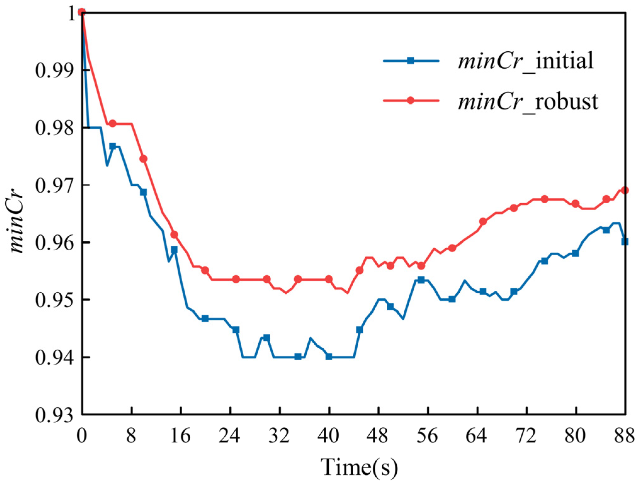
Experiments were performed based on the optimized design to obtain deformation measurement data. A total of 88 consecutive data points were acquired at 1-s intervals over an 88-s experimental period.

Figure 8 shows the curves of the clearance rates for the initial and optimized designs. The figure illustrates that the optimized design exhibits a consistently higher clearance rate than the initial design throughout the injection process. The initial clearance rate is 1. The minimum initial design clearance rate is approximately 0.94. The minimum robust design clearance rate is approximately 0.95. The minimum clearance rate of the optimized design is 1.2% greater than that of the initial design. The optimized design is confirmed to be better than the initial design. Therefore, the proposed method was validated as accurate and effective for optimization of the injection mechanism.

Figure 8. Clearance rate minCr of the initial and robust optimized designs in experiments.

5. Conclusions

This study proposes a 6σ robust optimization method based on a SPUTS hybrid metamodel, which significantly improves the prediction accuracy of optimized designs. Its effectiveness was validated through application to an injection mechanism with a large inner diameter. The main conclusions are as follows:

(1)

The hybrid metamodel, requiring only a small number of additional sample points, reduced the test set prediction error by 33.33% and the optimized design prediction error by 87.82% compared to the ordinary Kriging model.

(2)

The optimized design increased the system’s σ level to 4.87 times that of the initial design, indicating a substantial improvement in reliability. It also reduced the RMSE by 14.32% and increased the response mean by 1.58%, demonstrating enhanced robustness.

(3)

Experimental results showed that the optimized design achieved a higher clearance rate throughout the injection process, with a minimum clearance rate 1.2% greater than the initial design.

Limitations and Future Work: The hybrid Kriging–RBF metamodel was validated for a specific cold-chamber die casting setup and may not generalize to other systems (e.g., hot-chamber or multi-slide molds) without retraining. Training relies on costly finite element simulations, hindering real-time use, and assumes idealized material behavior and boundary conditions, ignoring real-world uncertainties like thermal fluctuations and wear. Future work will explore (1) transfer learning for rapid adaptation to new geometries, (2) multi-fidelity modeling to reduce simulation costs, and (3) robust multi-objective optimization that balances reliability, productivity, and energy efficiency under uncertainty.

References

1. Lelièvre, N.; Beaurepaire, P.; Mattrand, C.; Gayton, N.; Otsmane, A. On the consideration of uncertainty in design: Optimization-reliability-robustness. Struct. Multidiscip. Optim. 2016, 54, 1423–1437. [Google Scholar] [CrossRef]
2. Nie, J.; Zhong, S. Distributionally Robust Optimization with Polynomial Robust Constraints. J. Glob. Optim. 2025, 92, 509–534. [Google Scholar] [CrossRef]
3. Wei, N.; Zhang, P. Adjustability in robust linear optimization. Math. Program. 2024, 208, 581–628. [Google Scholar] [CrossRef]
4. Yu, H.; Yang, J.; Ding, X.; Wang, H.; Wang, S. Six sigma robust optimization method based on a pseudo single-loop strategy and RFR-DBN with insufficient samples. Comput. Struct. 2021, 257, 106653. [Google Scholar] [CrossRef]
5. Nejlaoui, M.; Alghafis, A.; Sadig, H. Six sigma robust multi-objective design optimization of flat plate collector system under uncertain design parameters. Energy 2022, 239, 121883. [Google Scholar] [CrossRef]
6. Liu, W.; Yang, Y.; Zheng, R.; Wang, P. Robust optimization for suspension parameters of suspended monorail vehicle using Taguchi method and kriging surrogate model. J. Chin. Soc. Mech. Eng. 2019, 40, 481–489. [Google Scholar]
7. Wang, P.; Yang, Y.; Yi, B.; Zeng, W.; Wang, T. Robust optimization of high-speed rail vehicle suspension parameters based on vertical running stability. J. Chin. Soc. Mech. Eng. 2019, 40, 583–593. [Google Scholar]
8. Du, Y.; Gu, J.; Zhang, H.; Hua, W. Reliability-based robust optimization of high-speed PM synchronous machine with local surrogate model Strategy. IEEE Trans. Transp. Electrif. 2024, 10, 9679–9690. [Google Scholar] [CrossRef]
9. Xiong, N.; Tao, Y.; Lin, J.; Liu, X.Q. Multi-levels Kriging surrogate model-based robust aerodynamics optimization design method. Int. J. Mod. Phys. B 2020, 34, 2040115. [Google Scholar] [CrossRef]
10. Xue, D.; Li, Y.; Zhang, H.; Tong, X.; Gao, B.; Yu, J. Reliability-based robust optimization design for tolerance of aerospace thin-walled components based on surrogate model. Adv. Eng. Inform. 2024, 62, 102754. [Google Scholar] [CrossRef]
11. Georgakis, C. Dynamic data-driven models for complex pharmaceutical reactions—The dynamic response surface methodology. Curr. Opin. Chem. Eng. 2024, 45, 101045. [Google Scholar] [CrossRef]
12. Haodong, L.I.U.; Jiang, H.; Sujun, D.O.N.G.; Longxian, X.U.E.; Yongji, L.I.U.; Jianjun, W.U. Simulation of an aircraft thermal management system based on vapor cycle response surface model. Chin. J. Aeronaut. 2024, 37, 64–77. [Google Scholar] [CrossRef]
13. He, Y.; Tan, K.; Fu, C.; Luo, J. An efficient gradient-enhanced kriging modeling method assisted by fast kriging for high-dimension problems. Int. J. Numer. Methods Heat Fluid Flow 2023, 33, 3967–3993. [Google Scholar] [CrossRef]
14. Appriou, T.; Rullière, D.; Gaudrie, D. High-dimensional Bayesian Optimization with a Combination of Kriging models. Struct. Multidiscip. Optim. 2024, 67, 196. [Google Scholar] [CrossRef]
15. Yamanaka, Y.; Matsubara, S.; Hirayama, N.; Moriguchi, S.; Terada, K. Surrogate modeling for the homogenization of elastoplastic composites based on RBF interpolation. Comput. Methods Appl. Mech. Eng. 2023, 415, 116282. [Google Scholar] [CrossRef]
16. Yang, X.; Zhang, Y.; Zhao, J.; Jiang, W. A novel active learning method based on matrix-operation RBF model for high-dimensional reliability analysis. Comput. Methods Appl. Mech. Eng. 2024, 432, 117434. [Google Scholar] [CrossRef]
17. Qosja, A.; Georges, D.; Gjika, E.; Nikolla, L.; Cela, A. A novel approach to electricity demand forecasting: An optimized Kalman filter-based RBF model. Int. J. Dyn. Control. 2025, 13, 165. [Google Scholar] [CrossRef]
18. Jin, R.; Du, X.; Chen, W. The use of metamodeling techniques for optimization under uncertainty. Struct. Multidiscip. Optim. 2003, 25, 99–116. [Google Scholar] [CrossRef]
19. Yondo, R.; Andrés, E.; Valero, E. A review on design of experiments and surrogate models in aircraft real-time and many-query aerodynamic analyses. Prog. Aerosp. Sci. 2018, 96, 23–61. [Google Scholar] [CrossRef]
20. Liu, X.; Hu, C.; Li, X.; Gao, J.; Huang, S. An online data-driven multi-objective optimization of a permanent magnet linear synchronous motor. IEEE Trans. Magn. 2021, 57, 8204804. [Google Scholar] [CrossRef]
21. Xie, G.; Zhao, C.; Li, H.; Du, W.; Liu, J.; Wang, Y.; Wang, H. A combination of extended finite element method and the Kriging model based crack identification method. Phys. Scr. 2023, 98, 115109. [Google Scholar] [CrossRef]
22. Li, S.; Wen, J.; Wang, J.; Liu, W.; Yuan, S. A high-precision surrogate modeling method based on parallel multipoint expected improvement point infill criteria for complex simulation problems. Mathematics 2022, 10, 3088. [Google Scholar] [CrossRef]
23. Gu, D.; Han, W.; Guo, J.; Guo, H.; Gao, S.; Liu, X. A Kriging-based adaptive adding point strategy for structural reliability analysis. Probabilistic Eng. Mech. 2023, 74, 103514. [Google Scholar] [CrossRef]
24. Chen, H.; Xu, C.; Li, Y.; Xu, C.; Su, H.; Guo, Y. An adding-points strategy surrogate model for well control optimization based on radial basis function neural network. Can. J. Chem. Eng. 2024, 102, 3514–3531. [Google Scholar] [CrossRef]
25. Wang, J.; Xia, G.; Li, R.; Ma, D.; Zhou, W.; Wang, J. Numerical simulation and microchannels parameters optimization for thermal management of GaN HEMT devices. Int. J. Numer. Methods Heat Fluid Flow 2021, 31, 2841–2861. [Google Scholar] [CrossRef]
26. Vural, N.; Yilmazer Hitit, Z.; Ertunç, S. Multi-objective optimization of drying conditions for the Olea europaea L. Leaves with NSGA-II. J. Food Process. Preserv. 2021, 45, e15625. [Google Scholar] [CrossRef]
27. Zhang, S.; Xu, F. A two-stage hybrid optimization for honeycomb-type cellular structures under out-of-plane dynamic impact. Appl. Math. Model. 2020, 80, 755–770. [Google Scholar] [CrossRef]
28. Fang, Z.; Tang, Z. Pareto equilibrium solution algorithm based on the metrics planning method and its application to multi-objective aerospace optimization. AIP Adv. 2025, 15, 035145. [Google Scholar] [CrossRef]
29. Lee, K.H.; Jeong, G.I.; Lee, S.H. An approximate optimization strategy using refined hybrid metamodel. Comput. Intell. 2020, 36, 35–54. [Google Scholar] [CrossRef]
30. Long, J.; Liao, Y.; Yu, P. Multi-response weighted adaptive sampling approach based on hybrid surrogate model. IEEE Access 2021, 9, 45441–45453. [Google Scholar] [CrossRef]
31. Lv, Y.; Lin, L.; Guo, H.; Tong, C.; Liu, Y.; Zhang, S.; Suo, S. An adaptive hybrid surrogate model for FEA of telescopic boom of rock drilling jumbo. Eng. Appl. Artif. Intell. 2024, 130, 107710. [Google Scholar] [CrossRef]
32. Srivastava, N.; Anas, M. An investigative review of squeeze casting: Processing effects & impact on properties. Mater. Today Proc. 2020, 26, 1914–1920. [Google Scholar]
33. Ghomashchi, M.R.; Vikhrov, A. Squeeze casting: An overview. J. Mater. Process. Technol. 2000, 101, 1–9. [Google Scholar] [CrossRef]
34. Yuanyuan, L.; Weiwen, Z.; Haidong, Z.; Dongdong, Y.; Datong, Z.; Ming, S.; Wen, Z. Research progress on squeeze casting in China. China Foundry 2014, 11, 239–246. [Google Scholar]
35. You, D.; Wang, X.; Cheng, X.; Jiang, X. Friction modeling and analysis of injection process in squeeze casting. J. Mater. Process. Technol. 2017, 239, 42–51. [Google Scholar] [CrossRef]
36. You, D.; Pang, W.; Li, F.; Zhu, Q. Thermohydrodynamic lubrication-based friction mechanism modeling and integrated simulation of dynamic coordination for squeeze casting processes. Int. J. Adv. Manuf. Technol. 2022, 120, 6481–6495. [Google Scholar] [CrossRef]
37. You, D.; Luo, X.; Zhu, Y.; Deng, J. Robust Optimization of Dynamic Fit Parameters for Injection Mechanism in Squeeze Casting Based on Six-sigma Frame and Bayesian Kriging Metamodel. Int. J. Met. 2023, 17, 124–142. [Google Scholar] [CrossRef]
38. Dargusch, M.S.; Hamasaiid, A.; Dour, G. An inverse model to determine the heat transfer coefficient and its evolution with time during solidification of light alloys. Int. J. Nonlinear Sci. Numer. Simul. 2008, 9, 275–282. [Google Scholar] [CrossRef]
39. Javidani, M.; Larouche, D. Application of cast Al–Si alloys in internal combustion engine components. Int. Mater. Rev. 2014, 59, 132–158. [Google Scholar] [CrossRef]
Disclaimer/Publisher’s Note: The statements, opinions and data contained in all publications are solely those of the individual author(s) and contributor(s) and not of MDPI and/or the editor(s). MDPI and/or the editor(s) disclaim responsibility for any injury to people or property resulting from any ideas, methods, instructions or products referred to in the content.
Article Metrics
Citations
Article Access Statistics
Multiple requests from the same IP address are counted as one view.