
Helical Electrodes for Electro-Discharge Drilling: Experimental and CFD-Based Analysis of the Influence of Internal and External Flushing Geometries on the Process Characteristics

 , and
, and
Abstract
1. Introduction
2. State of the Art
3. Materials and Methods
3.1. Experimental Setup for ED Drilling
3.2. Geometry Determination for Sophisticated 3D CFD Model
3.3. Generic Numerical Model and Approaches for Rotating Asymmetric Domains
- NV = 5 volume cells between opposite inflation layers across a gap, amongst others, was a necessary condition for the overset mesh approach;
- The inflation layer volume fraction amounted to about 50% of the working gap;
- The total number of cells NC needed to be as low as possible to enable a transfer of the meshing parameters to the even bigger mesh of the full numerical model;
- The dimensionless wall distance of the first cell should be in the order of y+ = 1.
- Component meshes of an overset interface may overlap arbitrarily, allowing them to be combined into a complex object, provided that physical boundary conditions, such as walls, an inlet or an outlet, do not intersect;
- However, component and background meshes can be placed in such a way that the physical boundary conditions lie on top of each other, and thus, e.g., wall boundary conditions can be coincident with each other;
- Overset boundary conditions, on the other hand, can intersect other overset boundary conditions, as well as physical boundary conditions;
- The calculation has to be performed with double precision;
- The time step selection for dynamic meshes must be based on the relative mesh motion per time step Δt, which should be below the smallest volume cell size lc of the overset interface.
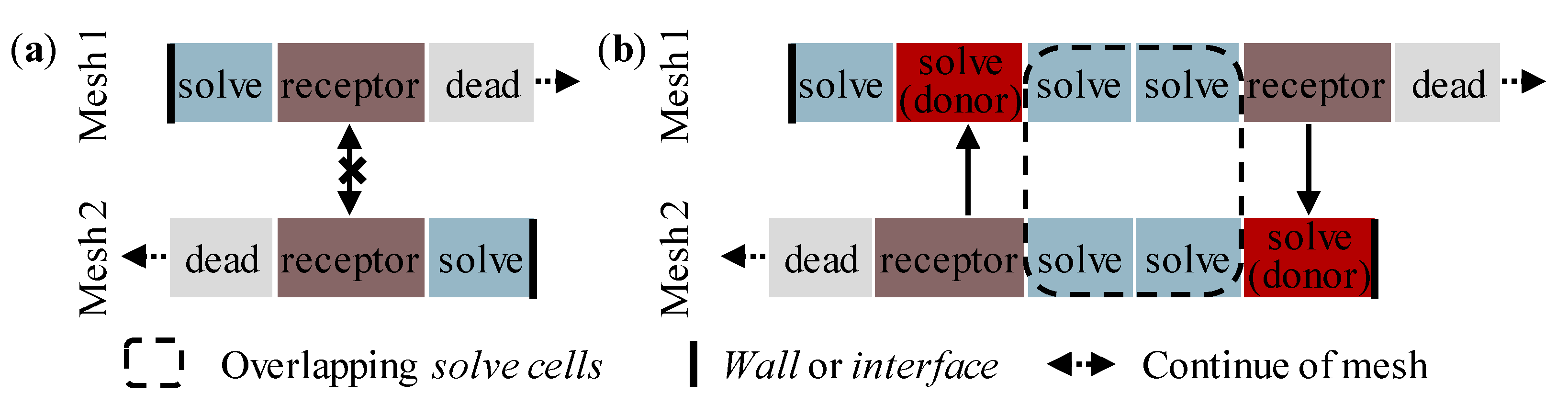
- Hole cutting: The process of marking mesh elements as dead cells that are outside of the fluid domain of interest, e.g., on the inside of bodies. Excessive overlap of component meshes and the background mesh is numerically inefficient. The transition of both meshes ideally occurs in areas with similar resolution. Large deviations between the overlapping meshes influence the interpolation, and thus, impair the quality of the solution.
- Overlap minimization: The process of converting solve cells to receptor cells, as well as unnecessary receptor cells in dead cells, between component meshes and the background mesh. A solve cell is converted into a receptor cell if a suitable donor cell with a higher donor quality can be found for this cell. The specification of a donor priority method influences this cell replacement procedure depending on the local mesh resolution.
- Donor search: A solve cell containing the centroid of a receptor cell of the overlapping mesh is used together with the adjacent solve cells as a donor for the selected receptor. Within the search, each receptor cell must be associated with at least one eligible donor or solve cell. Four or more cells must be present in the overlap zone of both meshes to ensure a successful donor search. Orphan cells are generated during initialization wherever this routine fails.

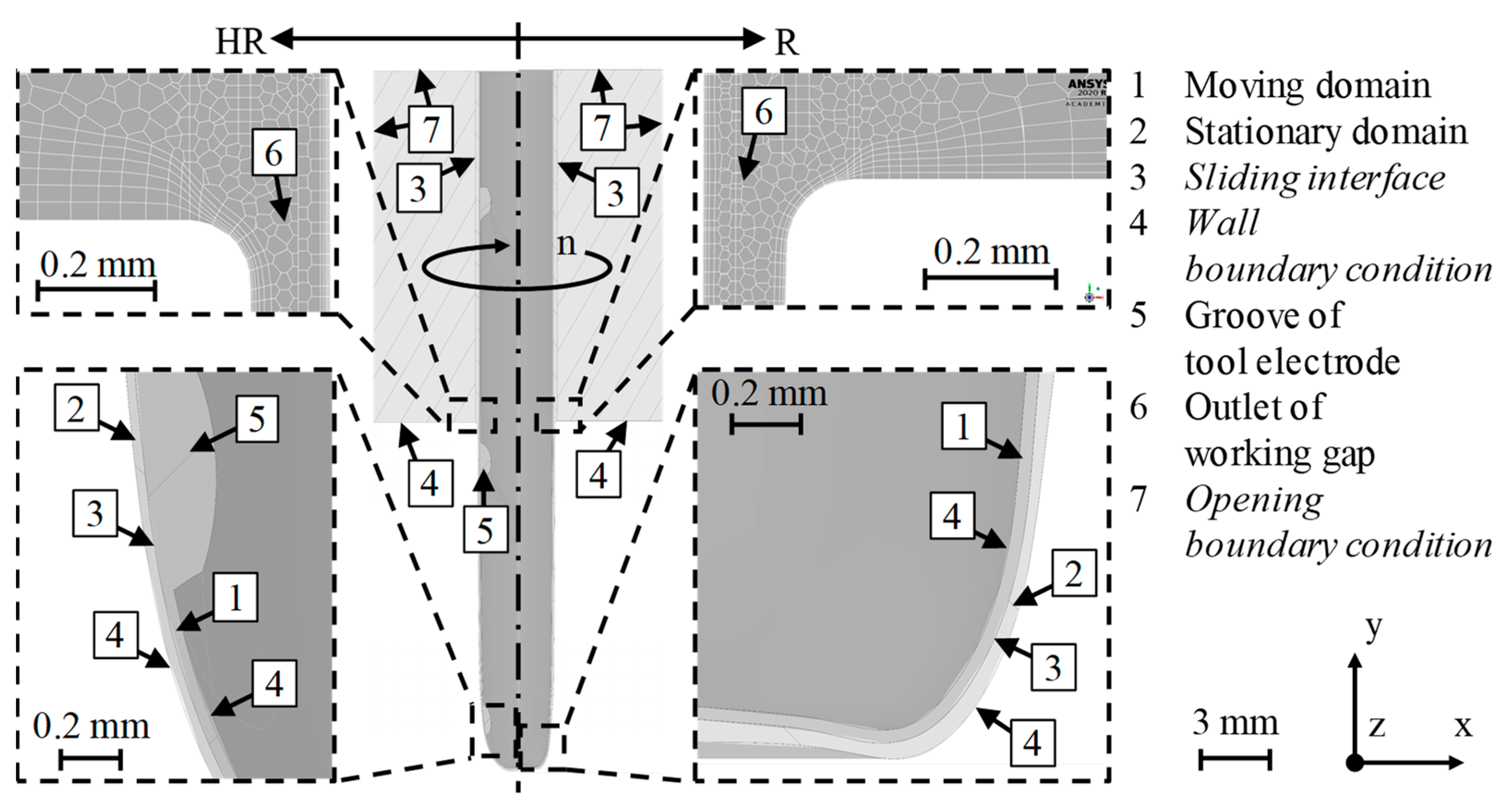
3.4. Sophisticated 3D CFD Model
- 50% of the cells across the working gap were volume cells;
- RANS modeling for the single-phase flow;
- Reference and operating pressure: pref = 0 MPa, pop = 0.1 MPa;
- Inlet pressure equaled the flushing pressure pf = 1.9 MPa;
- Moving domains rotated with rotational speed n = 400 min−1;
- Liquid only: neglected the presence of debris and gas bubbles;
- Steady-state solution after a number of iterations nI = 1000 iterations was followed by nR = 11 transient revolutions being calculated;
- Adaptive time step Δt for the first revolution to ensure CFL ≤ 1 (see Section 4.2);
- Last ten revolutions: fixed time step Δt = 0.00375 s; incremental angle passed: β = 9°; simulation durations tsim = 35 h for HR and tsim = 96 h for H1C.

| Mesh Characteristic | Value or Setting |
| Type of mesh | Poly-hexcore |
| Cell size in working gap | 20 µm ≤ lc ≤ 30 µm |
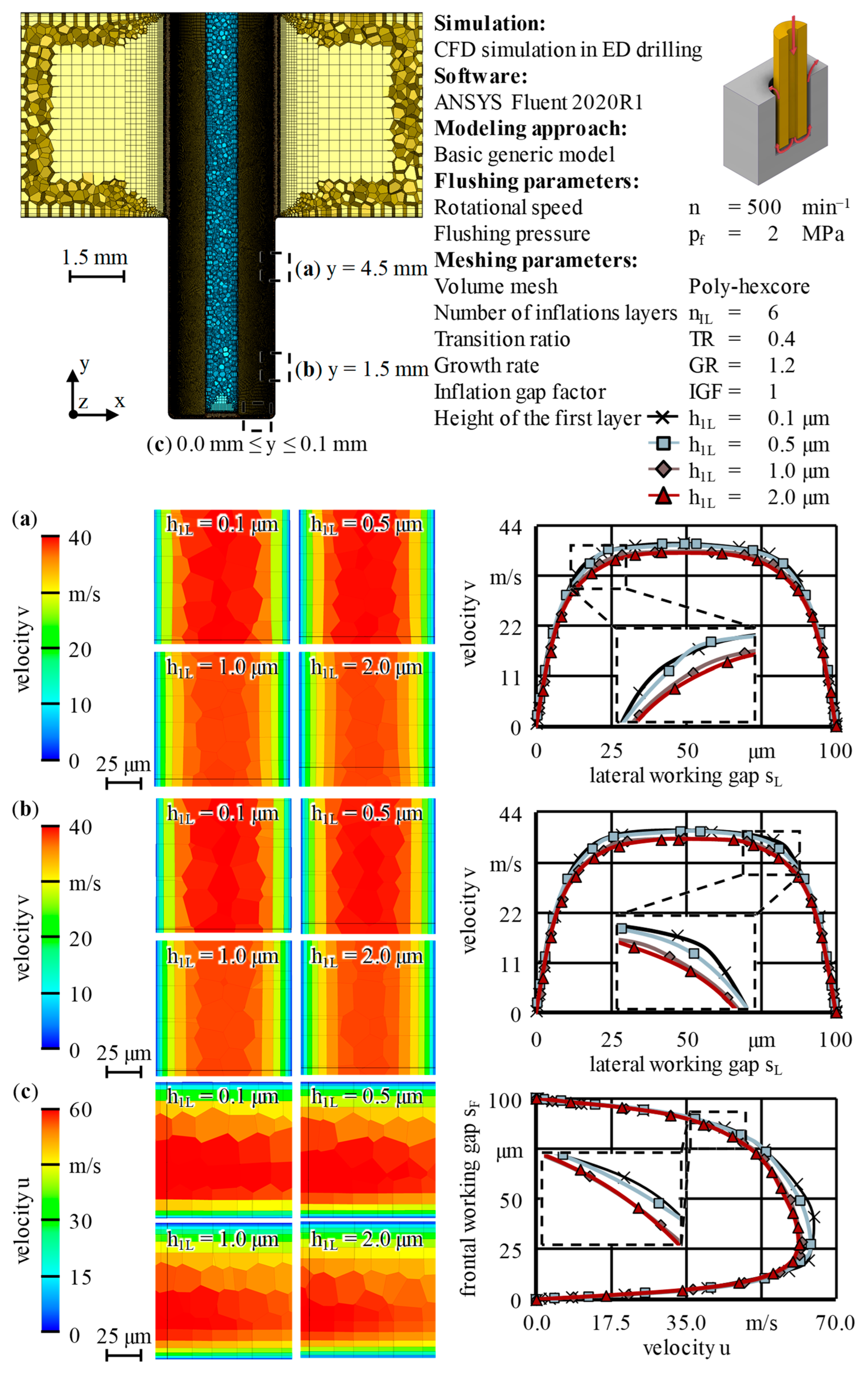
| Number of inflation layers | nIL = 6 |
| Height of the first layer | 0.5 µm ≤ h1L ≤ 10.0 µm |
| Total number of cells | 9.33 mil. ≤ NC ≤ 11.65 mil. |
| Model/Setting | Value or Setting |
| Turbulence | Realizable k-ε model, enhanced wall treatment |
| Pressure–velocity coupling | R, HR: SIMPLE; 1C, H1C, 4C, H4C: coupled |
| Spatial discretization | |
| Gradients | Least squares cell-based with warped-face gradient correction |
| Pressure | Second order |
| Momentum | Second-order upwind |
| Turbulent kinetic energy | First-order upwind |
| Turbulent dissipation rate | First-order upwind |
| Transient formulation | Steady: pseudo-time method global Transient: bounded second-order implicit |
| Time step | Δt = 0.00375 s |
| Iterations per time step | nI/Δt = 20 |
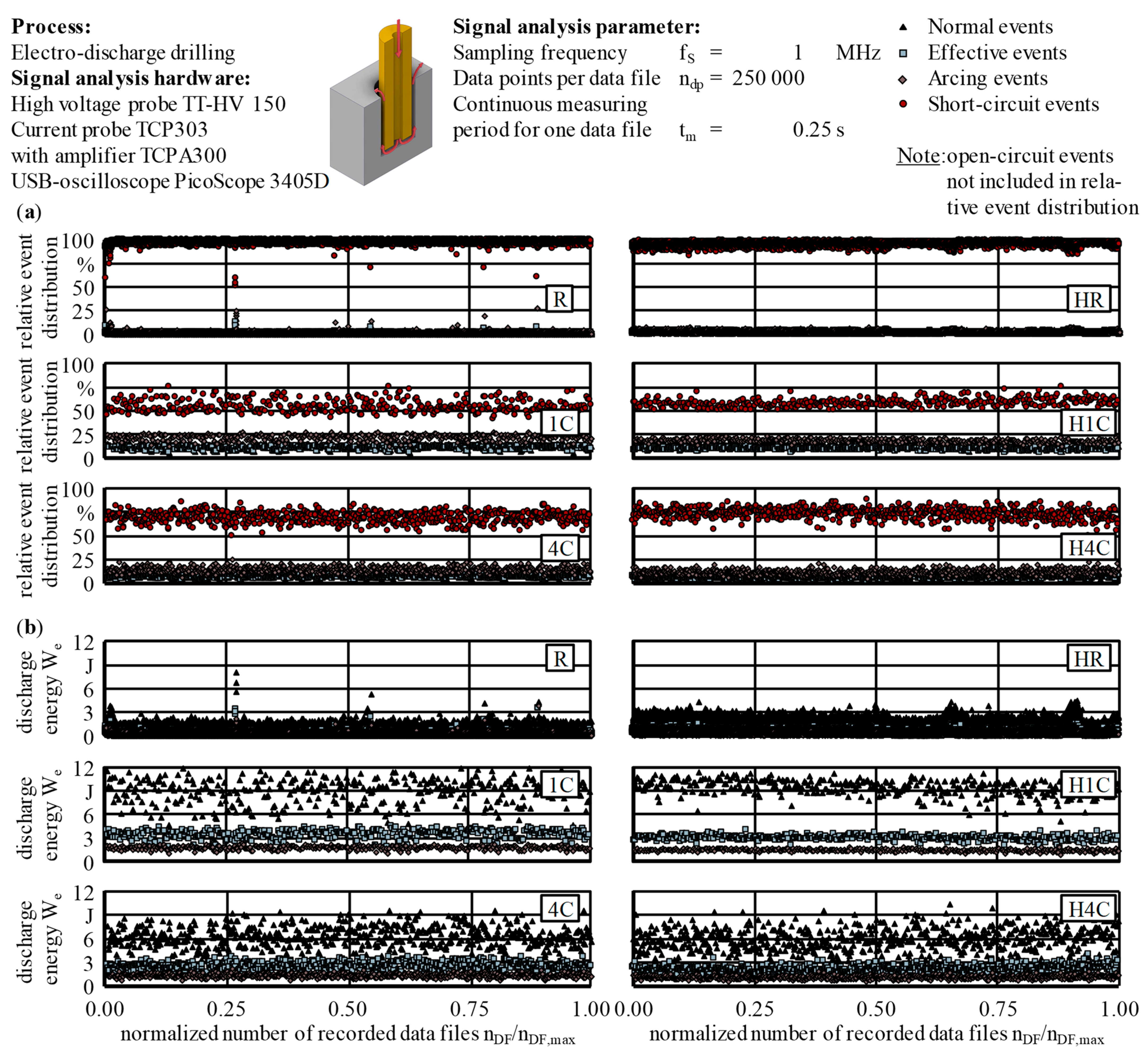
3.5. Signal Analysis
4. Results and Discussion
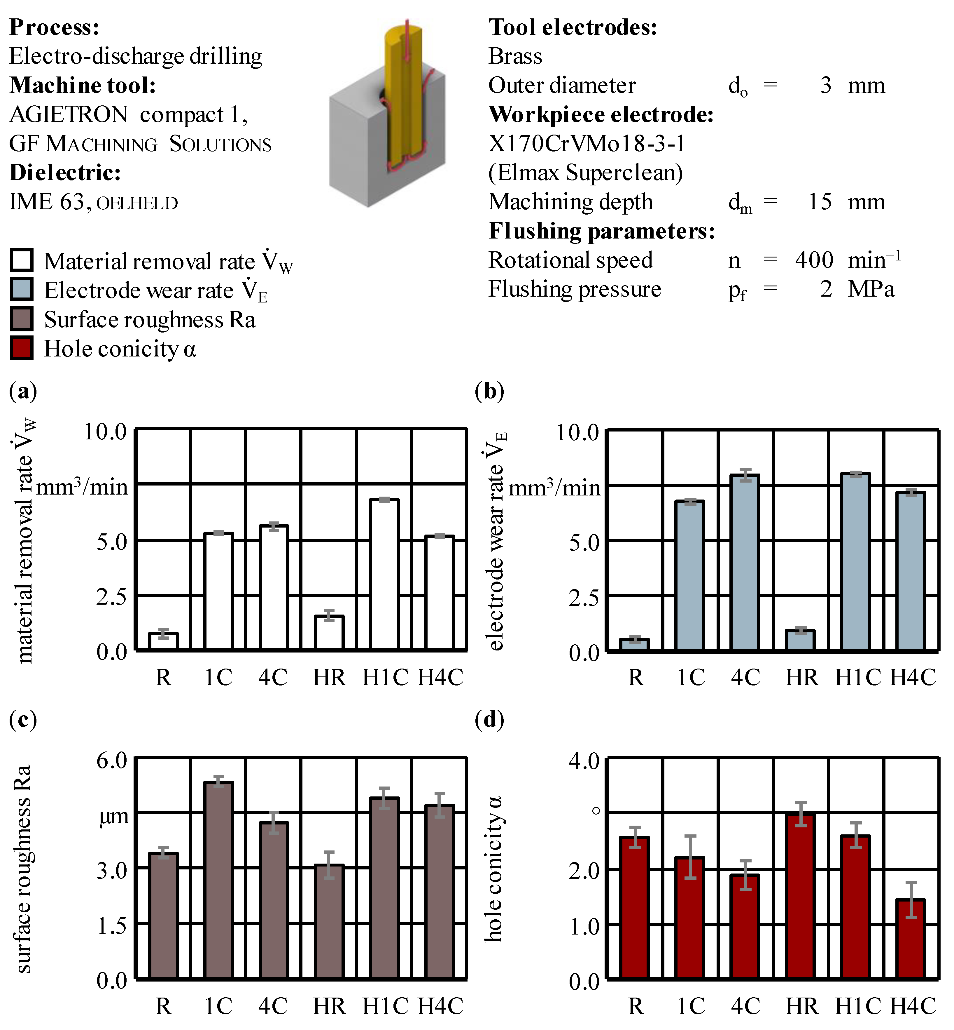
4.1. Experimental Results
- The additional external flushing channel geometry applied favored improvements in terms of MRR and surface roughness, but deteriorations in the EWR and the conicity for the R and 1C types while exhibiting the opposite behavior for the 4C types.
- The MRR increased by 112% when adding an external flushing channel to the R type, by 28% when adding it to the 1C type, but decreased by 8% in the case of the 4C type.
- Due to the relative frontal wear ϑIF, the beginning of the groove, and thus, its beneficial effect, were shifted upward for the HR type. Nevertheless, the bubble-flushing effect most probably generated sufficient additional lift from the tool electrode tip to push and pull removal products in the impact area of the groove.
- A precise comparison of the MRR and EWR between the six tool electrode types necessitated considering geometric differences in the greatest possible detail.
- The resulting pin geometries explained the comparison between 1C and 4C.
- Nevertheless, the effects of the altered frontal areas and flushing cross-sections on the process target parameters were superseded by the effects of cooling and direct ejection of the removal products as a result of the active high-pressure flushing.
4.2. Preliminary Numerical Results with the Generic Models
- Based on a basic 3D generic numerical model, the number of inflation layers and the height of the first layer were identified to be nIL = 6 and h1L = 0.5 µm to assure maximized numerical robustness and physical validity. These findings led to three more generic models to model the rotation of the asymmetric tool electrode geometry.
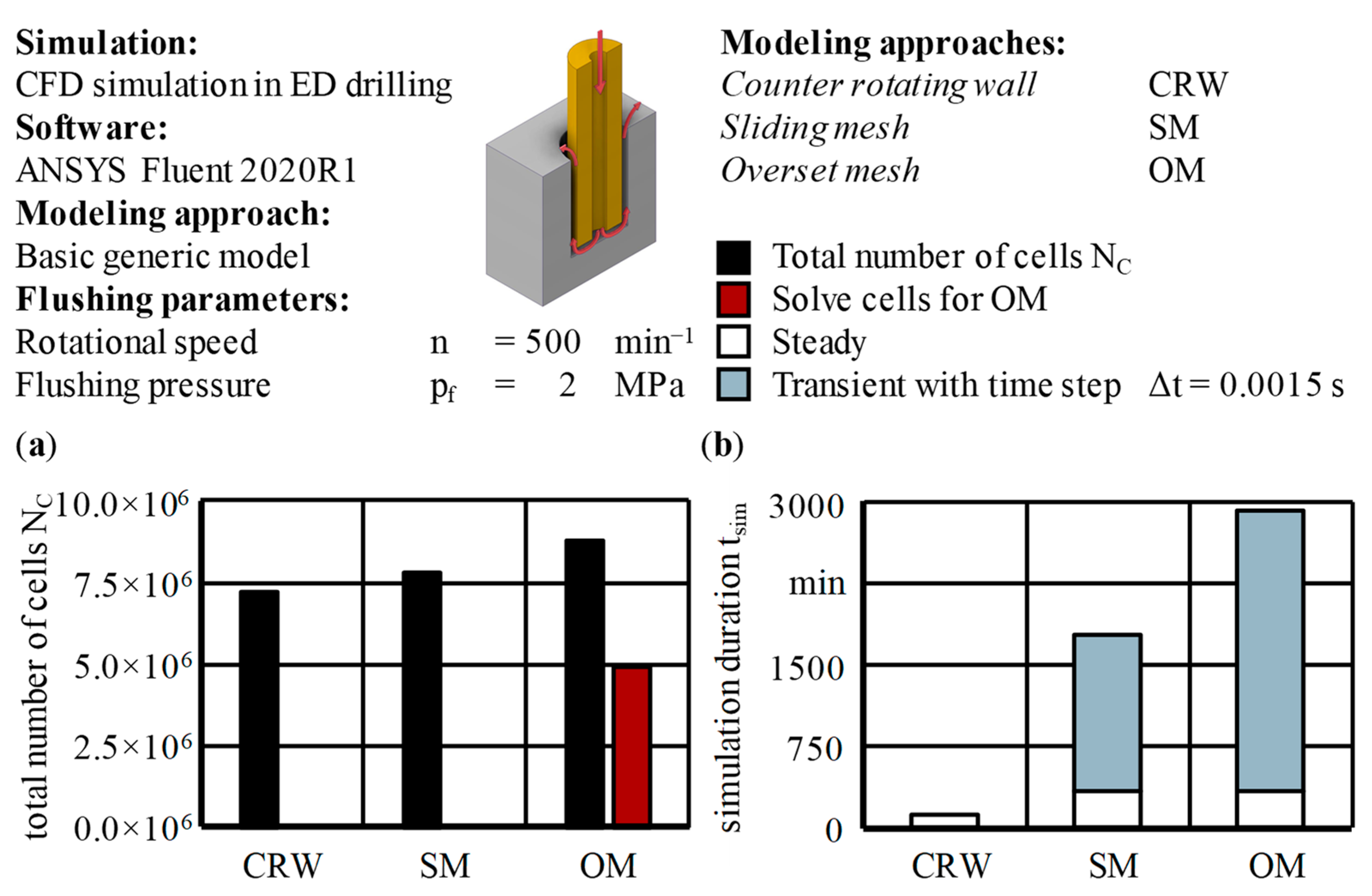
- The sliding mesh (SM) approach is the best trade-off between the mesh resolution and the accuracy of the solution based on generic numerical CFD models and compared against the two other techniques counter-rotating wall and overset mesh (OM). It holds the possibility to perform transient calculations and use greater time steps with less computation time.
4.3. Numerical Investigations of External Flushing Channels
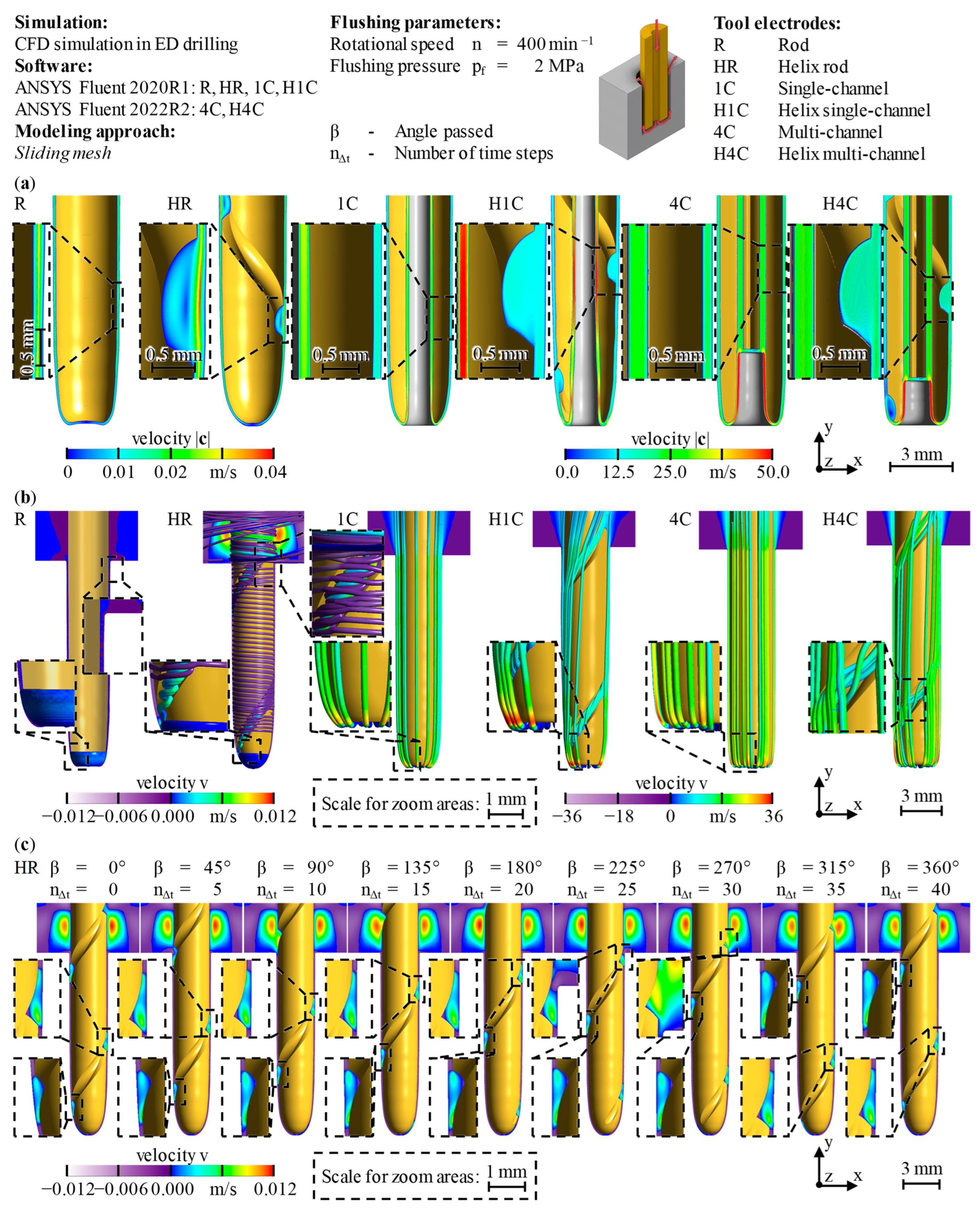
- A complex 3D CFD model using the SM approach ensured detailed numerical investigations of the fluid flow within the working gap in general and evaluations of the external flushing channel’s influence on the flow field for all six types of tool electrodes in particular.
- For the two rod types, the ratio of the axial to the radial velocity components showed the transformation of pure radial to a considerable upward-oriented axial movement of the dielectric as a result of the additional external flushing channel. Inside the groove, a downward-oriented fluid flow allowed fresh dielectric to enter the borehole.
- In the cases of the 1C and 4C types, most of the dielectric was directly and straight flushed out of the borehole with high vertical velocities, showing the dominance of the high flushing pressure over the rotational speed. In contrast, for the H1C and H4C types, the residence time of the dielectric in the working gap was prolonged, increasing the probability of fault discharges but also of the probably positive effect of shearing and scattering of gas bubbles and particle clusters.
- All types with an external flushing channel exhibited increased upward volume flow rates, as well as streamlines that followed the circumferential groove. However, some streamlines of the H1C and H4C types were pulled out of the groove, suggesting continuous spillover of fluid along the whole groove edge. Therefore, the need for adaptions of the fluid mechanical parameters specifically for each combination of groove angle and groove depth became evident. This has to be done in a way that means the ratio of the axial to the radial components of the main flow decreases so that gas bubbles and debris are pulled into the groove while being evacuated upwards.
- This is why the possibility of manipulating the velocity profiles on purpose was shown.
- An additional external flushing channel improved the pull effects in the area where particles and gas bubbles originated. The revealed tendencies coincided very well with the quantified experimental data in terms of the MRR and EWR. Also, the increase in the corresponding velocity ratio for the 4C compared with the 1C type was in good agreement, not only with the quantified upward volume flow rate but also with the experimental data.
4.4. Signal Analysis Results
- The R and HR types led to the lowest frequencies and frequency ratios of beneficials (see figure parts (a), (d) and (f)).
- Open circuits were driven by normals and effectives because of the corresponding charging cycles of fully or nearly full charged capacitors (see figure part (c)).
- The beneficial frequency ratio λben correlated with the MRR and the surface roughness Ra (see figure part (a) and Figure 12).
- The arcing frequency ratio λarc drove the EWR, in addition to the high energetic normal discharges (see figure part (e) and Figure 12).
- The normal frequency ratio λnorm correlated with the use of internal flushing and the flushing cross-section ratio Af/Ae (see figure parts (d) and (i)).
- The short-circuit frequency ratio λshort was slightly favored as a consequence of turbulences or radial velocity components |crad|, which were both primarily induced by multi-channel tool electrodes (1C → H1C, 4C → H4C) (see figure part (g) and Table 9). Furthermore, the streamlines for the H1C and H4C types in Figure 18b suggest continuous spillover of some fluid along the whole grooves edge as another reason for the systematic triggering of short circuits.
- The probability of detrimental events correlated with greater frontal areas Ae or smaller flushing cross-sections Af (see figure parts (b), (h) and (i)).
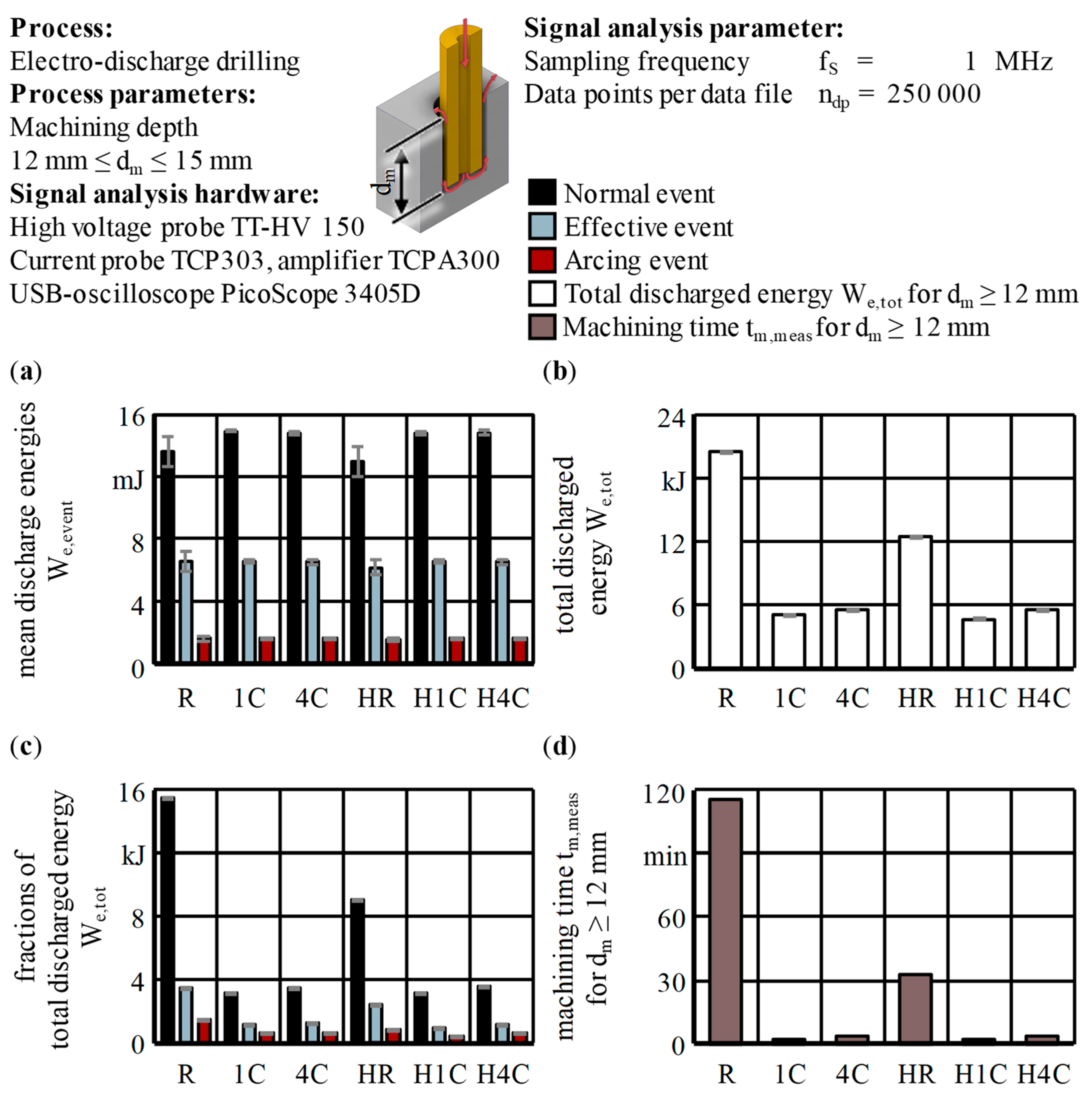
- Signal analyses of the gap voltage and current within the machining depth 12 mm ≤ dm ≤ 15 mm capturing 65% of all events allowed for a detailed event classification based on the edge detection and thresholds.
- Using performance-enhancing algorithms and techniques, the classification runtime could be reduced from 200 times the machining time down to 0.1 times the machining time of the actual drilling process, allowing for real-time signal analyses in principle.
- The R and HR types exhibited frequent early discharges as a result of accumulated particles that were bridging the working gap due to poor flushing conditions.
- Among other things, it was shown that the arcing frequency ratio defined the EWR, and the beneficial frequency ratio correlated with the MRR and the surface roughness.
- The short-circuit frequency ratio was favored as a consequence of turbulences or radial velocity components, like when using 4C or H4C tool electrodes or adding the additional external flushing channel.
- The probability of detrimental events correlated with greater frontal areas or smaller flushing cross-sections.
- The abstinence of active flushing led to numerous long sequences of open-circuit events as a result of frequent retraction movements of the feed axis.
- The frequencies of feed axis retractions as a result of arcing or short circuiting were calculated directly from the data of the signal analysis, revealing excellent agreement with the corresponding machining time over all types of tool electrodes.
- The causalities of an unstable process, and therefore, long machining time or low MRR with high values of the cumulative discharged energy were explained in light of the variable percentage shares of the real energy input being available for material removal, as well as the fact that the removal effects of distinguished discharge event types were influenced by the flow field’s gradients.
5. Conclusions and Outlook
- The additional external flushing channel geometry applied favored improvements in terms of the MRR and surface roughness, but deteriorations in the EWR and the conicity for the R and 1C types while exhibiting opposite behavior for the 4C types.
- The MRR increased by 112% when adding an external flushing channel to the R type and by 28% when adding it to the 1C type, but decreased by 8% in the case of the 4C type.
- The experimental results, especially when compared with the literature, underline the fact that generalized findings on internal flushing channels are difficult to deduce and are very case and geometry dependent. Consequentially, the same applies to external flushing channels and interdependencies with any kind of internal flushing.
- Single-phase simulations were sufficient for basic insights into the already complex flow field inside the working gap.
- Steady-state simulations were also sufficient for most basic analyses, like parameter studies on fluid mechanic parameters. Nevertheless, transient calculations were indispensable for the examination of transient effects, like multi-phase flow and phase interactions. However, transient calculations came with a vastly increased numerical cost, especially when performing parameter studies or two-way coupled two- or even three-phase calculations.
- However, the possibilities to explain any detail of the experimental results were, of course, limited. The major reasons for this were not only the imperfections of real experiments, like pressure fluctuations, spindle run-out errors, and the resulting low-pressure regions or tool electrode vibrations, but also the well-known limits and idealizations of numerical models, namely, perfect symmetry and constant boundary conditions, missing multi-phase considerations or the always limited validity of the models applied at any level, e.g., RANS approaches.
- It was not possible to draw direct, let alone linear, connections from the discharge energies to the process target parameters, such as the MRR, EWR, surface roughness or hole conicity. However, the classification and quantification of the discharge event types allowed for conclusions regarding their frequencies, and thus, the process stability.
- Amongst others, it was verified that the arcing frequency ratio drove the EWR and the beneficial frequency ratio correlated with the MRR and the surface roughness.
- External flushing channels verifiably led to convergence and reduced scattering of the relative event distributions
Supplementary Materials
Author Contributions
Funding
Data Availability Statement
Acknowledgments
Conflicts of Interest
References
- König, W.; Dauw, D.F.; Levy, G.; Panten, U. EDM-Future Steps towards the Machining of Ceramics. CIRP Ann. 1988, 37, 623–631. [Google Scholar] [CrossRef]
- Plaza, S.; Sanchez, J.A.; Perez, E.; Gil, R.; Izquierdo, B.; Ortega, N.; Pombo, I. Experimental study on micro EDM-drilling of Ti6Al4V using helical electrode. Precis. Eng. 2014, 38, 821–827. [Google Scholar] [CrossRef]
- Yu, Z.Y.; Rajurkar, K.P.; Shen, H. High Aspect Ratio and Complex Shaped Blind Micro Holes by Micro EDM. CIRP Ann. 2002, 51, 359–362. [Google Scholar] [CrossRef]
- Yu, Z.; Rajurkar, K.P.; Narasimhan, J. Effect of Machining Parameters on Machining Performance of Micro EDM and Surface Integrity. In Proceedings of the 18th Annual ASPE Meeting, Portland, OR, USA, 26–31 October 2003. [Google Scholar]
- Tsai, Y.-Y.; Masuzawa, T. An index to evaluate the wear resistance of the electrode in micro-EDM. J. Mater. Proc. Technol. 2004, 149, 304–309. [Google Scholar] [CrossRef]
- Cetin, S.; Okada, A.; Uno, Y. Effect of Debris Distribution on Wall Concavity in Deep-Hole EDM. JSME Int. J. Ser. C 2004, 47, 553–559. [Google Scholar] [CrossRef]
- Nastasi, R.; Koshy, P. Analysis and performance of slotted tools in electrical discharge drilling. CIRP Ann. 2014, 63, 205–208. [Google Scholar] [CrossRef]
- Jahan, M.P. Micro-Electrical Discharge Machining. In Nontraditional Machining Processes. Research Advances; Davim, J.P., Ed.; Springer: London, UK, 2013; pp. 111–151. [Google Scholar] [CrossRef]
- Flegel, G.; Birnstiel, K.; Nerreter, W.; Borcherding, H.; Meier, U. Elektrotechnik für Maschinenbau und Mechatronik, 10th ed.; Hanser: München, Germany, 2016. [Google Scholar]
- Klocke, F.; König, W. Fertigungsverfahren 3—Abtragen, Generieren Lasermaterialbearbeitung, 4th ed.; Springer: Berlin/Heidelberg, Germany, 2007. [Google Scholar]
- Uhlmann, E.; Polte, M.; Yabroudi, S. Novel Advances in Machine Tools, Tool Electrodes and Processes for High-Performance and High-Precision EDM. Procedia CIRP 2022, 113, 611–635. [Google Scholar] [CrossRef]
- Uhlmann, E.; Yabroudi, S.; Perfilov, I.; Schweitzer, L.; Polte, M. Helical electrodes for improved flushing conditions in drilling EDM of MAR-M247. In Proceedings of the 18th International Conference & Exhibition, Venice, Italy, 4–8 June 2018; Euspen: Bedford, UK, 2018; pp. 415–417. [Google Scholar]
- Yabroudi, S. Von ultrafein bis makro: Alternative Dielektrika sowie Elektrodenformen und -werkstoffe für das funkenerosive Bohren. In Proceedings of the 12th Fachtagung Funkenerosion, Aachen, Germany, 26–28 November 2019. [Google Scholar] [CrossRef]
- Yabroudi, S. Einsatzbewertung neuartiger Werkzeugelektroden mit außenliegenden Spülkanälen beim funkenerosiven Bohren mittels CFD Simulationen. In Proceedings of the 37th CADFEM ANSYS Simulation Conference, Kassel, Germany, 15–17 October 2019. [Google Scholar] [CrossRef]
- Thißen, K.; Streckenbach, J.; Koref, I.S.; Polte, M. Signal analysis on a single board computer for process characterisation in sinking electrical discharge machining. In Production at the Leading Edge of Technology; Behrens, B.A., Brosius, A., Drossel, W.G., Hintze, W., Ihlenfeldt, S., Nyhuis, P., Eds.; WGP 2021, Lecture Notes in Production Engineering; Springer: Cham, Switzerland, 2021; pp. 169–176. [Google Scholar] [CrossRef]
- Uhlmann, E.; Polte, J.; Streckenbach, J.; Dinh, N.C.; Yabroudi, S.; Polte, M.; Börnstein, J. High-Performance Electro-Discharge Drilling with a Novel Type of Oxidized Tool Electrode. J. Manuf. Mater. Proc. 2022, 6, 113. [Google Scholar] [CrossRef]
- Ferraris, E.; Castiglioni, V.; Ceyssens, F.; Annoni, M.; Lauwers, B.; Reynaerts, D. EDM drilling of ultra-high aspect ratio micro holes with insulated tools. CIRP Ann. 2013, 62, 191–194. [Google Scholar] [CrossRef]
- Takeuchi, H.; Kunieda, M. Relation between Debris Concentration and Discharge Gap Width in EDM Process. J. JSEME 2007, 41–98, 156–162. [Google Scholar] [CrossRef][Green Version]
- Takeuchi, H.; Kunieda, M. Relation between Debris Concentration and Discharge Gap Width in EDM Process. IJEM 2007, 12, 17–22. [Google Scholar]
- Kliuev, M.; Baumgart, C.; Wegener, K. Fluid Dynamics in Electrode Flushing Channel and Electrode-Workpiece Gap During EDM Drilling. Procedia CIRP 2018, 68, 254–259. [Google Scholar] [CrossRef]
- Yilmaz, O.; Okka, M.A. Effect of single and multi-channel electrodes application on EDM fast hole drilling performance. Int. J. Adv. Manuf. Technol. 2010, 51, 185–194. [Google Scholar] [CrossRef]
- Bozdana, A.T.; Ulutas, T. The Effectiveness of Multichannel Electrodes on Drilling Blind Holes on Inconel 718 by EDM Process. Mater. Manuf. Proc. 2016, 31, 504–513. [Google Scholar] [CrossRef]
- Bozdana, A.T.; Al-Kharkhi, N.K. Comparative Experimental and Numerical Investigation on Electrical Discharge Drilling of AISI 304 using Circular and Elliptical Electrodes. J. Mech. Eng. 2018, 64, 269–279. [Google Scholar] [CrossRef]
- Yan, B.H.; Huang, F.Y.; Chow, H.M.; Tsai, J.Y. Micro-hole machining of carbide by electric discharge machining. J. Mater. Proc. Technol. 1999, 87, 139–145. [Google Scholar] [CrossRef]
- Goiogana, M.; Elkaseer, A. Self-Flushing in EDM Drilling of Ti6Al4V Using Rotating Shaped Electrodes. Materials 2019, 12, 989. [Google Scholar] [CrossRef]
- Hirao, A.; Gotoh, H.; Tani, T. Effect of Electrode Shape on High Aspect Ratio Deep Hole Drilling by EDM. Procedia CIRP 2022, 113, 262–266. [Google Scholar] [CrossRef]
- Kumar, R.; Singh, I. Productivity improvement of micro EDM process by improvised tool. Prec Eng. 2018, 51, 529–535. [Google Scholar] [CrossRef]
- Kumar, R.; Singh, I. A modified electrode design for improving process performance of electric discharge drilling. J. Mater. Proc. Technol. 2019, 264, 211–219. [Google Scholar] [CrossRef]
- Manikandaprabu, P.; Kumar Thakur, D.; Sathish Kumar, M.; Sivanesh Prabhu, M.; Ramesh Kumar, A. Study and analysis of various inclination pathway electrode tool in electrical discharge drilling. Mater. Today Proc. 2021, 43, 1215–1219. [Google Scholar] [CrossRef]
- Kumar, R.; Singh, I. Blind Hole Fabrication in Aerospace Material Ti6Al4V Using Electric Discharge Drilling: A Tool Design Approach. J. Mater. Eng. Perform. 2021, 30, 8677–8685. [Google Scholar] [CrossRef]
- Nguyen, D.; Volgin, V.; Lyubimov, V. Modeling Electrical Discharge Machining of Deep Micro-Holes by Rotating Tool-Electrode. In Proceedings of the 6th International Conference on Industrial Engineering (ICIE 2020), Sochi, Russia, 18-22 May 2021; Radionov, A.A., Gasiyarov, V.R., Eds.; Springer International Publishing: Cham, Switzerland, 2021; pp. 171–179. [Google Scholar] [CrossRef]
- Takezawa, H.; Toyoda, H.; Yuasa, K. Effects of Thin Pipe Electrodes with Grooves in Small Deep Hole EDM. IJEM 2021, 26, 46–53. [Google Scholar] [CrossRef]
- Yadav, V.K.; Singh, R.; Kumar, P.; Dvivedi, A. Performance enhancement of rotary tool near-dry EDM process through tool modification. J. Braz. Soc. Mech. Sci. Eng. 2021, 43, 72. [Google Scholar] [CrossRef]
- Natsu, W.; Miyamoto, T.; Li, S. Clarification and Solution of Depth-dependent Tool Wear and Removal Rate in Micro Electrical Discharge Drilling. In Proceedings of the 13th International Conference of the EUSPEN, Berlin, Germany, 27–31 May 2013; EUSPEN: Bedford, UK, 2013; pp. 149–153. [Google Scholar]
- Machida, M.; Natsu, W. Flow analysis of working fluid in micro electrical discharge drilling process. In Proceedings of the 14th euspen International Conference & Exhibition, Dubrovnik, Croatia, 2–6 June 2014; EUSPEN: Bedford, UK, 2014; pp. 107–111. [Google Scholar]
- Risto, M.; Munz, M.; Haas, R.; Abdolahi, A. Securing a robust electrical discharge drilling process by means of flow rate control. In Proceedings of the 20th International ESAFORM Conference on Material Forming, Dublin, Ireland, 26–28 April 2017; p. 050007. [Google Scholar] [CrossRef]
- Wang, Z.; Gong, H.; Fang, F. Micro hole machining using double helix electrodes in electro discharge machining. J. Cent. South Univ. (Sci. Technol.) 2015, 46, 2857–2862. [Google Scholar]
- Wang, K.; Zhang, Q.; Zhu, G.; Liu, Q.; Huang, Y. Experimental study on micro electrical discharge machining with helical electrode. Int. J. Adv. Manuf. Technol. 2017, 93, 2639–2645. [Google Scholar] [CrossRef]
- Hu, Y.; Wang, H.; Wang, Z. Influence of helical electrode and its structure on EDM small hole machining. Int. J. Adv. Manuf. Technol. 2022, 123, 3437–3453. [Google Scholar] [CrossRef]
- Tsui, H.-P.; Hung, J.-C.; You, J.-C.; Yan, B.-H. Improvement of Electrochemical Microdrilling Accuracy Using Helical Tool. Mater. Manuf. Proc. 2008, 23, 499–505. [Google Scholar] [CrossRef]
- Hung, J.; Liu, H.; Chang, Y.; Hung, K.; Liu, S. Development of Helical Electrode Insulation Layer for Electrochemical Microdrilling. Procedia CIRP 2013, 6, 373–377. [Google Scholar] [CrossRef][Green Version]
- Fang, X.; Zhang, P.; Zeng, Y.; Qu, N.; Zhu, D. Enhancement of performance of wire electrochemical micromachining using a rotary helical electrode. J. Mater. Proc. Technol. 2016, 227, 129–137. [Google Scholar] [CrossRef]
- Liu, Y.; Wei, Z.; Wang, M.; Zhang, J. Experimental investigation of micro wire electrochemical discharge machining by using a rotating helical tool. J. Manuf. Proc. 2017, 29, 265–271. [Google Scholar] [CrossRef]
- Hung, J.-C.; Lin, J.-K.; Yan, B.-H.; Liu, H.-S.; Ho, P.-H. Using a helical micro-tool in micro-EDM combined with ultrasonic vibration for micro-hole machining. J. Micromech. Microeng. 2006, 16, 2705–2713. [Google Scholar] [CrossRef]
- Hsue, A.W.-J.; Chang, Y.-F. Toward synchronous hybrid micro-EDM grinding of micro-holes using helical taper tools formed by Ni-Co/diamond Co-deposition. J. Mater. Proc. Technol. 2016, 234, 368–382. [Google Scholar] [CrossRef]
- Hinduja, S.; Kunieda, M. Modelling of ECM and EDM processes. CIRP Ann. 2013, 62, 775–797. [Google Scholar] [CrossRef]
- Uhlmann, E.; Perfilov, I.; Yabroudi, S.; Mevert, R.; Polte, M. Dry-ED milling of micro-scale contours with high-speed rotating tungsten tube electrodes. Procedia CIRP 2020, 95, 533–538. [Google Scholar] [CrossRef]
- Yabroudi, S. CFD-Simulation in Mikrospülkanälen beim funkenerosiven Feinbohren mit flüssigen und gasförmigen Dielektrika. In Proceedings of the 35th CADFEM ANSYS Simulation Conference, Koblenz, Germany, 15–17 November 2017. [Google Scholar] [CrossRef]
- Uhlmann, E.; Frost, T.; Piltz, S.; Szulczynski, H. Strömungssimulation von Bearbeitungsprozessen. Neue Potentiale für die Fertigungstechnik von morgen. Wt Werkstattstech. Online 2001, 91, 320–324. [Google Scholar] [CrossRef]
- Brito Gadeschi, G.; Schneider, S.; Mohammadnejad, M.; Meinke, M.; Klink, A.; Schröder, W.; Klocke, F. Numerical Analysis of Flushing-Induced Thermal Cooling Including Debris Transport in Electrical Discharge Machining (EDM). Procedia CIRP 2017, 58, 116–121. [Google Scholar] [CrossRef]
- Brito Gadeschi, G.; Schneiders, L.; Meinke, M.H.; Schroeder, W. Direct particle-fluid simulation of flushing in die-sink electrical-discharge machining. In Proceedings of the 23rd AIAA Computational Fluid Dynamics Conference, Denver, CO, USA, 5–9 June 2017; American Institute of Aeronautics and Astronautics: Reston, VA, USA, 2017; p. 3619. [Google Scholar] [CrossRef]
- Schneiders, L.; Meinke, M.; Schröder, W. Direct particle–fluid simulation of Kolmogorov-length-scale size particles in decaying isotropic turbulence. J. Fluid. Mech. 2017, 819, 188–227. [Google Scholar] [CrossRef]
- Langmack, M. Laserwendel-und funkenerosives Mikrobohren. Ph.D. Thesis, TU Berlin, Berlin, Germany, 11 July 2014. [Google Scholar]
- Kliuev, M.; Baumgart, C.; Büttner, H.; Wegener, K. Flushing Velocity Observations and Analysis during EDM Drilling. Procedia CIRP 2018, 77, 590–593. [Google Scholar] [CrossRef]
- Wang, Y.Q.; Cao, M.R.; Yang, S.Q.; Li, W.H. Numerical Simulation of Liquid-Solid Two-Phase Flow Field in Discharge Gap of High-Speed Small Hole EDM Drilling. AMR 2008, 53–54, 409–414. [Google Scholar] [CrossRef]
- Pontelandolfo, P.; Haas, P.; Perez, R. Particle Hydrodynamics of the Electrical Discharge Machining Process. Part 2: Die Sinking Process. Procedia CIRP 2013, 6, 47–52. [Google Scholar] [CrossRef][Green Version]
- Wang, D. Simulation of Particles Movement in Powder Mixed EDM. AMR 2010, 97–101, 4150–4153. [Google Scholar] [CrossRef]
- Wang, J.; Han, F. Simulation model of debris and bubble movement in electrode jump of electrical discharge machining. Int. J. Adv. Manuf. Technol. 2014, 74, 591–598. [Google Scholar] [CrossRef]
- Wang, J.; Han, F. Simulation model of debris and bubble movement in consecutive-pulse discharge of electrical discharge machining. Int. J. Mach. Tools Manuf. 2014, 77, 56–65. [Google Scholar] [CrossRef]
- Zhang, S.; Zhang, W.; Liu, Y.; Ma, F.; Su, C.; Sha, Z. Study on the Gap Flow Simulation in EDM Small Hole Machining with Ti Alloy. Adv. Mater. Sci. Eng. 2017, 2017, 8408793. [Google Scholar] [CrossRef]
- Wang, Z.; Tong, H.; Li, Y.; Li, C. Dielectric flushing optimization of fast hole EDM drilling based on debris status analysis. Int. J. Adv. Manuf. Technol. 2018, 97, 2409–2417. [Google Scholar] [CrossRef]
- Klocke, F.; Herrig, T.; Zeis, M.; Klink, A. Modeling and simulation of the fluid flow in wire electrochemical machining with rotating tool (wire ECM). In Proceedings of the 20th International ESAFORM Conference on Material Forming, Dublin, Ireland, 26–28 April 2017; p. 50014. [Google Scholar] [CrossRef]
- Klocke, F.; Zeis, M.; Heidemanns, L. Fluid structure interaction of thin graphite electrodes during flushing movements in sinking electrical discharge machining. CIRP J. Manuf. Sci. Technol. 2018, 20, 23–28. [Google Scholar] [CrossRef]
- Xia, W.; Zhang, Y.; Chen, M.; Zhao, W. Study on Gap Phenomena Before and After the Breakout Event of Fast Electrical Discharge Machining Drilling. J. Manuf. Sci. Eng. 2020, 142, 041004. [Google Scholar] [CrossRef]
- Li, G.; Natsu, W.; Yu, Z. Elucidation of the mechanism of the deteriorating interelectrode environment in micro EDM drilling. Int. J. Mach. Tools Manuf. 2021, 167, 103747. [Google Scholar] [CrossRef]
- Izquierdo, B.; Wang, J.; Sánchez, J.A.; Ayesta, I. Study of particle size and position on debris evacuation during Wire EDM operations. IOP Conf. Ser. Mater. Sci. Eng. 2021, 1193, 12022. [Google Scholar] [CrossRef]
- Dauw, D.F.; Snoeys, R.; Dekeyser, W. Advanced Pulse Discriminating System for EDM Process Analysis and Control. CIRP Ann. 1983, 32, 541–549. [Google Scholar] [CrossRef]
- Uhlmann, E.; Polte, M.; Yabroudi, S.; Thißen, K.; Penske, W. Real-time energy monitoring in electrical discharge machining. Wt Werkstattstech. Online 2023, 113, 304–310. [Google Scholar] [CrossRef]
- Nirala, C.K.; Saha, P. Evaluation of μEDM-drilling and μEDM-dressing performances based on online monitoring of discharge gap conditions. Int. J. Adv. Manuf. Technol. 2016, 85, 1995–2012. [Google Scholar] [CrossRef]
- Nirala, C.K.; Unune, D.R.; Sankhla, H.K. Virtual Signal-Based Pulse Discrimination in Micro-Electro-Discharge Machining. J. Manuf. Sci. Eng. 2017, 139, 094501. [Google Scholar] [CrossRef]
- Janardhan, V.; Samuel, G.L. Pulse train data analysis to investigate the effect of machining parameters on the performance of wire electro discharge turning (WEDT) process. Int. J. Mach. Tools Manuf. 2010, 50, 775–788. [Google Scholar] [CrossRef]
- Zhou, M.; Han, F.; Soichiro, I. A time-varied predictive model for EDM process. Int. J. Mach. Tools Manuf. 2008, 48, 1668–1677. [Google Scholar] [CrossRef]
- Yeo, S.H.; Aligiri, E.; Tan, P.C.; Zarepour, H. A New Pulse Discriminating System for Micro-EDM. Mater. Manuf. Proc. 2009, 24, 1297–1305. [Google Scholar] [CrossRef]
- Bellotti, M.; Qian, J.; Reynaerts, D. Breakthrough phenomena in drilling micro holes by EDM. Int. J. Mach. Tools Manuf. 2019, 146, 103436. [Google Scholar] [CrossRef]
- Petersen, T.; Küpper, U.; Klink, A.; Herrig, T.; Bergs, T. Discharge energy based optimisation of sinking EDM of cemented carbides. Procedia CIRP 2022, 108, 734–739. [Google Scholar] [CrossRef]
- Schneider, S. Modellierung der Energiedissipation in der Funkenerosion. Ph.D. Thesis, RWTH, Aachen, Germany, 7 July 2021. [Google Scholar]
- Küpper, U.; Herrig, T.; Klink, A.; Welling, D.; Bergs, T. Evaluation of the Process Performance in Wire EDM Based on an Online Process Monitoring System. Procedia CIRP 2020, 95, 360–365. [Google Scholar] [CrossRef]
- Chu, H.-Y.; Li, Z.-L.; Xi, X.-C.; Zhao, W.-S. Study on Adaptive Servo Control Strategy of WEDM Based on Discharge State Detector. Procedia CIRP 2020, 95, 354–359. [Google Scholar] [CrossRef]
- Chu, H.-Y.; Zhang, M.; Xi, X.-C.; Li, Z.-L.; Zhao, W.-S. Observation of molten material and recast layer distribution of fast EDM drilling on inclined surface. Procedia CIRP 2022, 113, 250–255. [Google Scholar] [CrossRef]
- Schwade, M. Fundamental Analysis of High Frequent Electrical Process Signals for Advanced Technology Developments in W-EDM. Procedia CIRP 2014, 14, 436–441. [Google Scholar] [CrossRef][Green Version]
- Schwade, M. Automatisierte Analyse hochfrequenter Prozesssignale bei der funkenerosiven Bearbeitung von Magnesium für die Medizintechnik. Ph.D. Thesis, RWTH, Aachen, Germany, 20 April 2017. [Google Scholar]
- Schlichting, H.; Gersten, K. Grenzschicht-Theorie, 10th ed.; Springer: Berlin/Heidelberg, Germany, 2006; pp. 517–524. [Google Scholar]
- Schwarze, R. CFD-Modellierung, 1st ed.; Springer: Berlin/Heidelberg, Germany, 2013; pp. 134–155. [Google Scholar]
- ANSYS Inc. ANSYS Fluent Theory Guide, 2020R1 ed.; Ansys Inc.: Canonsburg, PA, USA, 2020. [Google Scholar]
- ANSYS Inc. ANSYS Fluent User’s Guide, 2020R1 ed.; Ansys Inc.: Canonsburg, PA, USA, 2020. [Google Scholar]
- Thißen, K.; Yabroudi, S.; Uhlmann, E. Localization of discharges in drilling EDM through segmented workpiece electrodes. In Production at the Leading Edge of Technology; Liewald, M., Verl, A., Bauernhansl, T., Möhring, H.C., Eds.; WGP 2022. Lecture Notes in Production Engineering; Springer: Cham, Switzerland, 2022; pp. 209–218. [Google Scholar] [CrossRef]
- Li, X.; Wang, Y.; Liu, Y.; Zhao, F. Research on Shape Changes in Cylinder Electrodes Incident to Micro-EDM. Adv. Mater. Sci. Eng. 2019, 2019, 8087462. [Google Scholar] [CrossRef]
- Tu, J.; Liu, C.; Yeoh, G.H. Computational Fluid Dynamics. A practical Approach, 3rd ed.; Butterworth-Heinemann: Oxford, UK, 2018; pp. 220–222. [Google Scholar] [CrossRef]
- Oßwald, K.; Schneider, S.; Hensgen, L.; Klink, A.; Klocke, F. Experimental investigation of energy distribution in continuous sinking EDM. CIRP J. Man. Sci. Technol. 2017, 19, 36–43. [Google Scholar] [CrossRef]
- Kunieda, M.; Lauwers, B.; Rajurkar, K.P.; Schumacher, B.M. Advancing EDM through Fundamental Insight into the Process. CIRP Ann. 2005, 54, 64–87. [Google Scholar] [CrossRef]
- Li, G.; Natsu, W.; Yu, Z. Observation of phenomena in gap area during micro hole drilling with micro EDM. In Proceedings of the 17th International Conference & Exhibition, Hannover, Germany, 29 May–2 June 2017; EUSPEN: Bedford, UK, 2017; pp. 195–196. [Google Scholar]
- Haas, R.; Munz, M.; Huber, M.; Knabe, R. Adequate Gap Flushing in High Speed EDM Drilling of Deep Small Holes in Moulds and Dies. In Proceedings of the 7th International Conference on High Speed Machining (CIRP), Darmstadt, Germany, 28–29 May 2008; Abele, E., Ed.; Meisenbach Verlag: Bamberg, Germany, 2008. [Google Scholar]


| Parameter | Unit | Value |
|---|---|---|
| Rotational speed n | min−1 | 400.00 |
| Flushing pressure pf | MPa | 2.00 |
| Polarity of tool electrode | - | Negative |
| Open circuit voltage ûi | V | 180.00 |
| Charge current iL | A | 4.00 |
| Discharge capacity Ce | µF | 1.32 |
| Pulse duration ti | µs | 18.00 |
| Pulse interval time t0 | µs | 2.40 |
| Resulting discharge current ie | A | <125.00 |
| Compression | - | 40.00 |
| Gain | - | 15.00 |
| Parameter | Unit | Values | |||||
|---|---|---|---|---|---|---|---|
| Number of inflation layers nIL | - | 3 | 6 | 9 | |||
| Height of the first layer h1L | µm | 0.1 | 0.5 | 1.0 | 2.0 | ||
| Mesh Characteristic | CRW | SM | OM |
| Type of mesh | Poly-hexcore | ||
| Number of inflation layers | nIL = 6 | ||
| Height of the first layer | h1L = 0.5 µm | ||
| Dimensionless wall distance | y+ = 1.39 | ||
| Model/Setting | CRW | SM | OM |
| Turbulence | Realizable k-ε model, enhanced wall treatment | ||
| Pressure–velocity coupling | SIMPEL | PISO | Coupled |
| Spatial discretization | |||
| Gradients | Least squares cell-based, with warped-face gradient correction | ||
| Pressure | Second order | ||
| Momentum | Second-order upwind | ||
| Turbulent kinetic energy | First-order upwind | ||
| Turbulent dissipation rate | First-order upwind | ||
| Transient formulation | - | Bounded second-order implicit | |
| Time step | - | Δt = 0.0015 s | |
| Parameter | Unit | Dielectric IME63 | Air |
|---|---|---|---|
| Density ρ | kg/m3 | 770 | 1.2250 |
| Dynamic viscosity µ × 10−5 | kg/m·s | 138.6 | 1.7894 |
| Surface tension coefficient γ | mN/m | 24.11 | |
| Parameter | Value | Parameter | Value | Parameter | Value |
|---|---|---|---|---|---|
| y(P1) | 0.0 | y(P6) | 12.0 | di | 1.2 |
| y(P2) | 0.4 | y(P7) | 15.0 | sF | 0.1 |
| y(P3) | 3.0 | le | 45.0 | sL | 0.1 |
| y(P4) | 6.0 | dm | 15.0 | ||
| y(P5) | 9.0 | do | 3.0 | All values in mm. | |
| Threshold | Classified as | Comment |
|---|---|---|
| u ≥ 0.72 ûi | Normal | Peak discharge energy We observed at 72% of ûi |
| 0.50 ûi ≤ u < 0.72 ûi | Effective | Capacitor not fully charged due to contamination |
| 0.30 ûi ≤ u < 0.50 ûi | Arcing | Grouped events with low amplitude of ûi |
| u < 0.30 ûi | Short circuit | Electrodes bridged |
| Thresholds | Classified as | Comment | |
|---|---|---|---|
| - | i < ith | Open circuit | No contribution, loading of capacitor |
| u ≥ 0.85 × ûi | i ≥ ith | Normal | Capacitor fully or mostly charged |
| 0.45 × ûi ≤ u < 0.85 × ûi | i ≥ ith | Effective | Early capacitor discharges |
| 0.16 × ûi ≤ u < 0.45 × ûi | i ≥ ith | Arcing | Mostly series of low energetic events |
| u < 0.16 × ûi | i ≥ ith | Short circuiting | Electrodes bridged |
| Assumed | |||||||||
|---|---|---|---|---|---|---|---|---|---|
| Comparison | Ae | Af | tm | MRR | EWR | Ra | α | Reasons | |
| R | → 1C | ↓ 18.2 | - | ↓ 91.0 | ↑ 612.2 | ↑ 1406.6 | ↑ 56.4 | ↓ 13.8 | I, VI |
| R | → 4C | ↓ 12.6 | - | ↓ 90.5 | ↑ 652.3 | ↑ 1704.5 | ↑ 24.0 | ↓ 26.9 | I, V, VI |
| HR | → H1C | ↓ 19.6 | ↑ 255.3 | ↓ 80.1 | ↑ 331.2 | ↑ 934.7 | ↑ 58.2 | ↓ 12.8 | I, VI |
| HR | → H4C | ↓ 13.6 | ↑ 177.3 | ↓ 71.3 | ↑ 228.7 | ↑ 826.6 | ↑ 52.0 | ↓ 52.0 | I, V, VI |
| R | → HR | ↓ 7.1 | - | ↓ 63.8 | ↑ 111.6 | ↑ 75.3 | ↓ 9.4 | ↑ 16.2 | III, IV, V |
| 1C | → H1C | ↓ 8.7 | ↑ 39.2 | ↓ 20.0 | ↑ 28.1 | ↑ 18.8 | ↓ 8.4 | ↑ 17.6 | II, IV |
| 4C | → H4C | ↓ 8.1 | ↑ 56.4 | ↑ 9.4 | ↓ 7.6 | ↓ 10.0 | ↑ 11.0 | ↓ 23.8 | II, IV |
| 1C | → 4C | ↑ 6.8 | ↓ 30.6 | ↑ 5.8 | ↑ 5.6 | ↑ 18.2 | ↓ 20.8 | ↓ 15.1 | IV, V |
| H1C | → H4C | ↑ 7.4 | ↓ 22.0 | ↑ 44.7 | ↓ 23.8 | ↓ 10.4 | ↓ 4.0 | ↓ 45.0 | IV, V |
| I II III IV V VI | Removal of debris by pressure flushing Additional space for debris and gas bubbles Removal of debris and gas bubbles through external flushing channel Change in frontal area Ae and flushing cross-section Af Turbulences or radial velocity components |crad| Improved cooling of the discharge zones | Legend: ↑ Increase ↓ Decrease ↕ Improvement ↕ Deterioration All values in %. | |||||||
| Number of Inflation Layers nIL | Total Number of Cells NC | Height of First Layer h1L | Maximum Value of y+ |
|---|---|---|---|
| 3 | 5 088 770 | 0.1 µm | 0.28 |
| 6 | 6 539 346 | 0.5 µm | 1.39 |
| 9 | 7 976 085 | 1.0 µm | 2.62 |
| 2.0 µm | 5.45 |
| Unit | R | 1C | 4C | HR | H1C | H4C | ||
|---|---|---|---|---|---|---|---|---|
| Total machining time tm | min | 206.49 | 18.59 | 19.66 | 74.81 | 14.87 | 21.51 | |
| Signal analysis | Machining depth dm | mm | 12 mm ≤ dm ≤ 15 mm | |||||
| Recorded data files nDF | - | 17 874 | 356 | 565 | 4834 | 338 | 617 | |
| Machining time tm,meas | min | 115.35 | 2.33 | 3.68 | 33.10 | 2.20 | 4.07 | |
| % | 55.86 | 12.51 | 18.72 | 44.24 | 14.78 | 18.91 | ||
| Measuring duration tmeas | min | 75 735 | 1524 | 2406 | 20 609 | 1442 | 2664 | |
| Measurement ratio rmeas | - | 0.66 | 0.66 | 0.65 | 0.62 | 0.66 | 0.65 | |
| Event distribution | Normals | - | 1 147 217 | 212 941 | 238 003 | 702 313 | 215 513 | 245 836 |
| Effectives | - | 543 280 | 185 396 | 203 171 | 404 750 | 152 392 | 185 874 | |
| Arcing | - | 966 262 | 384 848 | 426 850 | 576 127 | 308 187 | 385 593 | |
| Short circuiting | - | 98 248 159 | 954 695 | 1 910 751 | 25 263 371 | 942 904 | 2 222 987 | |
| Open circuits | - | 118 140 952 | 2 624 900 | 4 145 300 | 32 294 109 | 2 523 194 | 4 521 045 | |
Disclaimer/Publisher’s Note: The statements, opinions and data contained in all publications are solely those of the individual author(s) and contributor(s) and not of MDPI and/or the editor(s). MDPI and/or the editor(s) disclaim responsibility for any injury to people or property resulting from any ideas, methods, instructions or products referred to in the content. |
© 2023 by the authors. Licensee MDPI, Basel, Switzerland. This article is an open access article distributed under the terms and conditions of the Creative Commons Attribution (CC BY) license (https://creativecommons.org/licenses/by/4.0/).
Share and Cite
Uhlmann, E.; Polte, M.; Yabroudi, S.; Gerhard, N.; Sakharova, E.; Thißen, K.; Penske, W. Helical Electrodes for Electro-Discharge Drilling: Experimental and CFD-Based Analysis of the Influence of Internal and External Flushing Geometries on the Process Characteristics. J. Manuf. Mater. Process. 2023, 7, 217. https://doi.org/10.3390/jmmp7060217
Uhlmann E, Polte M, Yabroudi S, Gerhard N, Sakharova E, Thißen K, Penske W. Helical Electrodes for Electro-Discharge Drilling: Experimental and CFD-Based Analysis of the Influence of Internal and External Flushing Geometries on the Process Characteristics. Journal of Manufacturing and Materials Processing. 2023; 7(6):217. https://doi.org/10.3390/jmmp7060217
Chicago/Turabian StyleUhlmann, Eckart, Mitchel Polte, Sami Yabroudi, Nicklas Gerhard, Ekaterina Sakharova, Kai Thißen, and Wilhelm Penske. 2023. "Helical Electrodes for Electro-Discharge Drilling: Experimental and CFD-Based Analysis of the Influence of Internal and External Flushing Geometries on the Process Characteristics" Journal of Manufacturing and Materials Processing 7, no. 6: 217. https://doi.org/10.3390/jmmp7060217
APA StyleUhlmann, E., Polte, M., Yabroudi, S., Gerhard, N., Sakharova, E., Thißen, K., & Penske, W. (2023). Helical Electrodes for Electro-Discharge Drilling: Experimental and CFD-Based Analysis of the Influence of Internal and External Flushing Geometries on the Process Characteristics. Journal of Manufacturing and Materials Processing, 7(6), 217. https://doi.org/10.3390/jmmp7060217