Abstract
In conventional forming processes, quasi-static conditions are a good approximation and numerical process optimization is the state of the art in industrial practice. Nevertheless, there is still a substantial need for research in the field of identification of material parameters. In production technologies with high forming velocities, it is no longer acceptable to neglect the dependency of the hardening on the forming speed. Therefore, a method for determining material characteristics in processes with high forming speeds was developed by designing and implementing a test setup and an inverse parameter identification. Two acceleration concepts were realized: a pneumatically driven one and an electromagnetically driven one. The method was verified for a mild steel and an aluminum alloy proving that the identified material parameters allow numerical modeling of high-speed processes with good accuracy. The determined material parameters for steel show significant differences for different stress states. For specimen geometries with predominantly uniaxial tensile strain at forming speeds in the order of 104–105/s the determined yield stress was nearly twice as high compared to shear samples; an effect which does not occur under quasi-static loading. This trend suggests a triaxiality-dependent rate dependence, which might be attributed to shear band induced strain localization and adiabatic heating.
1. Introduction
1.1. Motivation
High forming velocities can provide significant technological advantages in manufacturing processes such as increased formability, improved quality of cutting edges, reduced springback, etc. [1]. Therefore, realizing challenging manufacturing tasks and processing complex materials including modern lightweight materials such as aluminum or magnesium becomes possible via special techniques using these velocity effects. This allows for new products with improved quality and reduced product weight. Thus, it is possible to save resources and reduce emissions, especially in the transport sector, but also in other applications including moving masses such as the manufacturing sector, energy generation sector and many more.
Despite these advantages, the corresponding technologies, which are often referred to as high-speed forming, impulse forming or high-energy-rate-forming (HERF) [2] have not yet achieved a great industrial breakthrough. Reasons for this are lacking process knowledge and reliable process design strategies. When considering conventional forming processes, it is possible to assume a close approximation of quasi-static conditions, and numerical process design and optimization as state of the art. By contrast, the analysis and design of manufacturing processes with high forming speeds has hitherto been strongly experimental. Numerical considerations are helpful to investigate fundamental relationships, but often only qualitative interpretation is possible. One reason for this is that material parameters are hardly available at the process-specific high strain rates in the range of 10 s−1 up to 105 s−1 or even more. The identification of these parameters is complicated, because in addition to the influencing factors known from quasi-static conditions such as temperature and strain, the plastic flow and failure behavior of many materials strongly depends on the strain rate. Therefore, neglecting forming heat, as well as a strain rate-dependent hardening is no longer acceptable. Providing a method for determining reliable material and failure characteristics for the simulation of high-velocity forming, cutting, and joining processes will therefore contribute to making technological, economic, and ecological advantages of these processes exploitable in industrial production.
1.2. State of the Art
1.2.1. High-Speed Technologies
In the literature, there is no unique and clear-cut definition of high-speed technologies. Lange classifies all processes that use stored energy to shape a workpiece in a very short time as high-speed forming processes [3]. Schüßler considers processes with cutting speeds of 0.8 m/s or more as high-speed cutting [4], while Bruno speaks of high-speed forming at a speed of 15 m/s or more [5]. According to Wielage and Vollertsen, strain rates in high-speed processes typically reach values of 102 to 107 s−1, while the process time is in the order of micro or milliseconds [6]. In principle, the specification of the strain rate is important in these processes, but a single scalar value is insufficient for the description because strains and strain rates vary temporally and locally. Specifically, electrically stored energy [7], chemically stored energy [8] and mechanically stored energy [9] can be used for realizing high-speed manufacturing processes (i.e., forming, joining, and cutting operations). The industry is currently taking strong interest especially in shaping, cutting, and joining by means of electromagnetic forming (EMF) and in cutting with accelerated tools.
In EMF, the workpiece must be in direct vicinity to a so-called tool coil (inductor). When discharging a capacitor via the inductor, a damped sinusoidal current flows that induces a corresponding magnetic field and a countercurrent in the workpiece. Due to the interactions between current and magnetic field, Lorentz forces cause acceleration and plastic deformation of workpiece areas when the resulting stresses in the material reach the yield stress. The major process variants of electromagnetic compression and expansion of pipes and hollow profiles as well as the electromagnetic deformation of plane or preformed sheets differ with regard to the geometry and arrangement of inductor and workpiece [7].
Shaping by EMF usually uses a form-defining die on the side of the workpiece facing away from the inductor. During the process, the workpiece aligns to the die cavity if machine parameters, workpiece parameters and tool–i.e., coil and die–parameters are appropriate [10]. Strain rates in shaping by EMF can reach values in the range of 103/s up to 104/s. Cutting by EMF requires a cutting tool on the side of the workpiece facing away from the inductor. The interaction with this cutting tool causes the desired material separation when the plastic strain reaches the material-specific elongation at break. In contrast to conventional cutting, where shearing occurs followed by shear fracture, the material separation in cutting by EMF can be attributed to bending followed by cracking [11]. For joining by EMF, three principle mechanisms are available based on interference-fit, form-fit, and magnetic pulse welding. In interference-fit joining, the acting force causes plastic deformation of the first and elastic deformation of the second joining partner. When the forces have decayed, the remaining plastic deformation of the first joining partner prevents complete reversal of the elastic deformation of the second one [12]. For form-fit joining, one joining partner features geometrical elements such as grooves or beads. During deformation, the other joining partner flows into these geometry elements and forms an undercut [13]. In magnetic pulse welding, the deformation causes a high-speed impact of the two joining partners. If collision parameters are appropriate, a so-called jet effect removes potential oxide layers and other surface contaminations from the collision zone. Supported by the contact pressure, the resulting clean and highly reactive surfaces form a metallically bonded joint [14]. Strain rates in this process variant can locally reach values in the range of 105/s up to 106/s. Combining EMF with conventional forming processes such as deep drawing [15], extrusion [16], bending [17] and hydroforming [18] frequently allows exploiting the complementary advantages of different production processes.
To achieve high process efficiency in EMF, workpieces must provide high electrical conductivity. EMF of insulating or poorly conductive materials requires a so-called driver, i.e., an additional element of highly electrically conductive material positioned between the inductor and the workpiece. This driver mechanically transmits the Lorentz force induced therein to the workpiece. Economically, however, this is hardly acceptable, so alternative drives, e.g., accelerated tools, are used [7]. For forming and cutting with accelerated tools, the following drive types exist:
- mechanical: high-speed presses (punch speed approx. 1.5 m/s [19])
- pneumatic: e.g., Dynapak (punch speed up to 16 m/s [20])
- hydraulic: e.g., Adiapress (punch speed up to 15 m/s [21])
- electromagnetic (punch speed up to 35 m/s [22])
- chemical or explosive: e.g., Petroforge (punch speed up to 32 m/s [23])
Advantages compared to conventional presses are that presses for forming and cutting with accelerated tools are compact, require relatively low investment costs, do not require elaborate foundations, and enable high production rates [9]. As an alternative to special high-speed machines, Yaldiz et al. developed an accelerator unit that can be used to adapt conventional presses to high-speed forming and separation processes [24]. In addition to forming and cutting processes, using electromagnetically driven tools is also possible for powder compaction [25].
1.2.2. Material Characterization at High Strain Rates
Industrial use of the described high-speed manufacturing methods requires reliable calculation tools and material data for feasibility assessments and process design. Different high-speed testing methods and machines serve for determining material data at high strain rates, which is necessary input data for these calculation tools. High-speed tensile and compression tests usually use fast servo-hydraulic testing machines to characterize material behavior under uniaxial tensile or compressive loading at speeds of up to 20 m/s [26] and forming speeds up to 102/s [27]. Abouridane uses them for the characterization of flow and fracture behavior of light alloys [28].
Drop weight impact testers use the kinetic energy of a falling weight for suddenly loading the specimen. Usually, the weight falls on a stationary sample, thus accelerating it. By contrast, in [29], the weight and the sample drop until they hit an anvil leading to abrupt deceleration. Drop-body-based setups enable speeds of up to 4 m/s [27] and strain rates of up to 103/s [30]. They are most suitable for pressure and bending tests, but also enable compression shear and biaxial tensile tests with strain rates of up to 103/s [31]. However, oscillations in the order of the magnitude of the measurement signal often complicate the interpretation of the measurement data if the drop weight directly carries the accelerometers.
Pendulum impact testers use the kinetic energy of a pendulum hammer for the impact loading of test specimens at speeds of up to 6 m/s. In addition to the usual applications for the determination of dynamic fracture toughness or notched impact work, modified structures are suitable for dynamic tensile and compression tests [27].
In rotational wheel impact testers, the sample’s movable chucking area is located near a flywheel, which accelerates to circumferential speeds of up to approx. 40 m/s. When it reaches the target speed, a claw loads the sample abruptly. Such structures are suitable for tensile tests, notched tensile tests and bending tests [32]. Halle uses a modified impact tester for hot tensile and torsion tests at high forming speeds [33].
The idea of using Hopkinson Bar setups goes back to 1914 [34]. Modern structures use the modification of the structure according to [35]. These setups usually consist of two long bars (incident bar and transmission bar) followed by a damping element, which clamp the specimen. Compressed air accelerates a so-called striker, which impacts with the incident bar. The resulting pulse travels through the specimen to the transmission bar. Strain gauges record the differences between the input and output pulses. This is the basis for calculating the corresponding characteristic material parameters for strain rates of up to 105/s for miniaturized structures [36].
In ring expansion and cylinder expansion tests, detonating explosives or EMF accelerate the ring- or tube-shaped specimens in radial outward direction. Strain rates of up to 104/s and large expansions are possible with a simple setup, but the test is limited to analyzing tensile loads [37].
In the plate impact test, an explosively driven projectile accelerates a so-called flyer plate to speeds of up to several kilometers per second. Measurements of the impact speed of the flyer plate and the particle velocity at the back (e.g., via laser interferometry) and the state of stress in the plate (e.g., via piezoelectric sensors) provide the basis for characterizing the material behavior for typically one-dimensional strain states and strain rates of up to 106/s [36]. Similarly, in the Taylor impact test, a high-speed bar collides with a plate or a second bar, resulting in dynamic deformation of bars or plates. The final geometry, which depends on the impact velocity and the material behavior, provides the basis for determining the material parameters via inverse parameter identification [36]. Table 1 gives an overview about existing high-speed testing methods and machines, comparing their advantages and limits.

Table 1.
Comparison of advantages and limits of different high-speed testing methods.
Due to the established use of the finite element analysis FEA, the inverse determination of process and material parameters has become very important. Especially in the field of manufacturing technology, a lot of work has been dedicated to such developments [38,39,40,41]. In the inverse approach, the relationship between effective loads (cause) and deformation behavior (effect) is determined using a deterministic numerical calculation method. However, in contrast to conventional simulation methods, the effect is available as temporally or locally measured parameters and deterministic calculation methods serve for identifying the associated cause via targeted variation of the input data. This input data can include the geometry, the effective loads but also the material parameters or the constitutive equation itself. A stable solution requires high sensitivity to slight variation of the parameters. At the same time, the change of the result must be small for minor changes of the input data [38]. Inverse methods always use an optimization algorithm that does not necessarily detect the global minimum and may provide a different solution if the starting values are changed. Thus, it is necessary to pay attention to the uniqueness of the obtained solution.
Nevertheless, there are many successful examples of inverse parameter identification in the fields of production engineering, mechanics, and materials science. Brunet et al. e.g., use the inverse method for determining the parameters for describing the kinematic hardening by means of a cyclic bending test [39]. Moments and deformations measured during cyclic bending of a narrow sheet metal strip serve for calculating the material parameters with a commercial optimization program.
Brosius uses a downhill simplex algorithm for flow curve determination in the inverse analysis of a tube tensile test. Here, the flow curve cannot be determined directly from the force-displacement curve, because the current cross section, which is necessary for determining the true stress, is unknown. Thus, a simple FE model serves for adapting the numerically determined force-displacement curve to the measurement by adjusting a hardening law with six parameters [42].
As mentioned above, the choice of a suitable material law is a major difficulty of the inverse parameter identification. The assumptions strongly influence its identification and an optimization algorithm is required in order to vary the free parameters purposefully. Gradient-based methods, also known as hill climbing methods, improve the target function value continuously and quickly, but a deterioration of the target function value is not possible, which is a disadvantage if the objective function has several local optima. Further improvement is possible only by restarting the algorithm with modified starting values since the convergence behavior depends on the starting vectors. Gradient-based methods converge very close to the optimum, since the objective function can be approximated by a quadratic curve. However, starting vectors far from the optimum, cause problems in the calculation of the gradients and lead to slowly converging problems [43]. In contrast, stochastic methods “scan” the parameter space within specified limits and determine the next solution vector. The convergence process is neither reproducible nor predictable. The essential advantage of these methods is the high probability of detecting the global minimum despite of unknown target function topology. The disadvantage is the required frequent evaluation of the objective function [44]. The gradient-based methods developed in [45] and [46] are recommended as standard methods to be used for solving non-linear least-squares problems because of their outstanding suitability and robustness e.g., in [47].
Altogether, analysis and design of manufacturing processes with high forming speeds has hitherto been strongly experimental. Numerical considerations serve for investigating fundamental relationships, but their interpretation is often possible in a qualitative manner only. One reason for this is that material characteristics are not available at the process-specific high forming speeds with sufficient accuracy. Existing machines and methods for material characterization are applicable only for a limited range of strain rates. Especially at high strain rates, the interpretation of the test result is extremely complex. Therefore, there is a need for a new method for determining material and failure characteristics for processes with high strain rates. The application of these characteristics allows accurate numerical modeling of high-speed forming and cutting processes, so that the numerical simulation becomes applicable for the process and tool design. This contributes significantly to the use of the known process-specific advantages in industrial production, and specifically in sheet metal forming.
2. Materials and Methods
To achieve this goal, a new test setup with accelerated tools and the corresponding evaluation strategy is developed, implemented, and tested for the steel material DC06 and the aluminum alloy EN-AW5754 H111 with a nominal thickness of 1.0 mm. Both materials are highly relevant for industrial applications. DC06 is a material with significant strain rate dependency whereas the strain rate sensitivity of EN-AW5754 H111 is usually is less distinctive. Different driving mechanisms serve for accelerating the tool in order to be able to set a range of strain rates from 101/s to 105/s and different sample geometries allow the realization of different stress states. Due to the high process speed and small sample size, it is not possible to detect the data relevant for the determination of the material and failure parameters directly. Therefore, auxiliary quantities are measured in order to characterize the acting loads and the resulting deformation. Numerical modeling supports the analysis and interpretation of test results. Inverse strategies help to identify material and failure parameters by adjusting the numerically determined load and displacement with the corresponding measured results. Finally, experiments verify the determined data. For this purpose, an electromagnetic sheet metal forming process is considered. Displacement over time curves are calculated for the identified material parameters at high strain rates and comparison to corresponding measured curves demonstrates the improvement of the simulation accuracy in relation to material parameters determined at quasi-static strain rates.
2.1. Specimen Design
To determine the material and failure characteristics under different load conditions, different sample geometries were designed and evaluated with regard to manufacturing feasibility and the expected stress states. With regard to the stress state it is important that
- the stress distribution in the considered specimen area is relatively homogeneous, although real homogeneity is not possible due to the dynamic character of any high-speed test, which results in stress waves in the specimen, and
- the desired loading direction, characterized by the value of the stress triaxiality, dominates in the considered specimen area.
Numerical parameter studies presented in [48] served for analyzing the stress state in the relevant test area of the specimen. They demonstrated that the considered geometries could cover a large area of stress from uniaxial pressure to the biaxial tension. This corresponds to triaxialities in the range of approx. −1/3 to approx. 2/3. The stress and strain paths are approximately linear over time.
Moreover, it is essential that the specimens can transfer a load up to the failure without significant buckling or bending. As laminated packages consisting of several sheet specimens offer increased buckling stability, the presented investigations regarded packages of four parallel sheets. In practical experiments, spot tests verified the applicability of the numerically designed specimens. Figure 1 compares exemplary specimen geometries with the respective test results and demonstrates that tensile specimens with higher widths s in the test area can transmit larger forces, which lead to stronger bending of the specimen. The numerical model in the inverse parameter identification considers this bending, and therefore it is not a limitation for the evaluation of the test. However, in extreme cases the maximum possible displacement dzmax (3.0 mm here) is achieved at significantly lower elongation in the test area, thus no failure of the sample occurs.
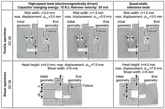
Figure 1.
Deformation of exemplary specimen geometries.
Particularly the head height h, the shear area b and the maximum possible displacement dzmax are decisive when considering specimen geometries for shear tests. When loading at high speed, a maximum possible displacement of 7 mm, a head height of 4 mm and a shear width of 5 mm are suitable to achieve failure in the test area for the regarded specimens. Comparative tests with quasi-static loading show that a stronger, unwanted bending occurs here, so that a larger head height is required in order to be able to make a direct comparison. By contrast, the regarded tensile specimen geometry with a web width of 1.5 mm and a maximum possible displacement of 3.0 mm is suitable for both dynamic tests and quasi-static reference experiments. Figure 2 shows the specimen geometries selected for the inverse characteristic determination within this study based on the numerical and experimental investigations.
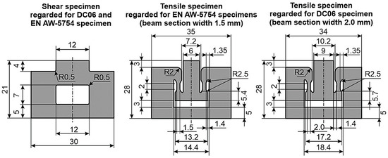
Figure 2.
Specimen geometries regarded in inverse parameter identification.
2.2. Experimental Setup and Measurement Technology
Two devices have been implemented which allow material parameters to be recorded at forming speeds of the order of 102/s to 105/s. Specifically, a pneumatically driven hammer was implemented for speeds of 102/s to 103/s and an electromagnetically driven hammer was implemented for forming speeds of 103/s to 105/s. The fine adjustment of the strain rates is possible by varying the active media pressure in case of the pneumatically driven tool, and by varying the capacitor charging voltage in case of the electromagnetically driven tool, on the one hand, and by modifying the mass of the accelerated tool, on the other hand.
2.2.1. Experimental Setup Using Pneumatically Driven Tools
The pneumatically driven device bases on a high-speed cutting device, first mentioned in [49] and enables material characterization in a conventional press at hammer speeds of 3 to 8 m/s. Depending on the geometry of the sample, strain rates of 0.5 × 10² to 1.2 × 10³ s−1 occur. The press stroke compresses air in the acceleration device until the hammer is triggered, and accelerates at high speed in the direction of the specimen. Figure 3 shows the principle setup of the device at significant process stages.
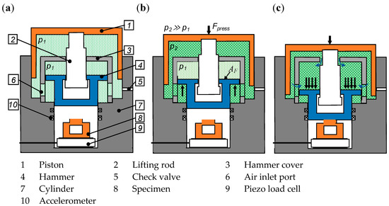
Figure 3.
Principle of the pneumatically driven acceleration unit according to [48]: (a) neutral position, (b) pressurization, (c) impact.
At the beginning of the process before the start of the stroke the air pressure in the acceleration unit is p1 (Figure 3a). During the press stroke, the piston and the lifting rod move downwards and compress the air to a pressure p2 in the piston chamber (Figure 3b) until the shoulder of the lifting rod sweeps over the hammer cover and opens the passage between piston chamber and hammer chamber. At that moment, the compressed air flows from the piston chamber into the hammer chamber. As a result, the high air pressure acts on the hammer flange AF and the hammer moves downwards. As soon as it passes the air inlet port, the highly compressed air flows abruptly into the hammer chamber, the counterforce, which presses against the hammer flange from below, drops to zero and the hammer is accelerated out of the hammer chamber and hits the specimen (Figure 3c). Finally, the press opens up and the remaining pressure lifts piston and hammer back into the initial position.
The design of the device bases on the assumption of an adiabatic change of state of the system. The adiabatic exponent is κ = 1.4 (air as medium). Figure 4 shows the dimensions for calculating the achievable hammer speed. For the change of state from Figure 3a to Figure 3c, Equation (1) results in the change of state in the piston.
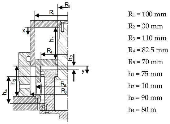
Figure 4.
Necessary measurements for calculating the hammer velocity.
At a filling pressure pini = 0.7 MPa, a piston pressure ppiston = 2.54 MPa results in the hammer chamber before the hammer passes through the air inlet port in the hammer cover. As soon as the hammer passes the air inlet port, the volumes of the piston chamber Vpiston depending on the displacement x of the piston and hammer chamber Vhammer combine to form a total volume Vtotal with a uniform pressure ptotal. Here Equation (2) applies.
Immediately after passing through the air intake ports, h2 = 40 mm and h4 = 50 mm, so that Equation (2) results in Equation (3).
Equation (4) calculates the reaction force Ftotal accelerating the hammer, taking into consideration the friction force Ffriction caused e.g., by the necessary sealing in the setup.
The hammer acceleration ahammer and velocity vhammer finally result from the hammer mass mhammer and the distance s of the hammer to the sample according to Equations (5) and (6).
To be able to characterize the acting loads and the deformation of the specimen during the testing procedure an acceleration sensor and a piezo-based load cell were implemented in the experimental setup. The acceleration sensor serves for recording the movement of the hammer, which works as an auxiliary variable for determining the displacement in the specimen. For this purpose, the acceleration signal is integrated twice over time to obtain the hammer displacement. Due to the complex kinematics of the pneumatically driven hammer, the force signal is essential, when detecting the stages of the hammer movement, precisely the acceleration and the deformation of the specimen as described in [50]. Figure 5 shows the experimental setup. For verification of the displacement measurement, the acceleration sensor, a laser shadowing method, and a digital image correlation (DIC) simultaneously recorded the process. The measurement results of DIC and shadowing method are very similar. The deviation of the measurement curve determined by the accelerometer is due to the low stiffness of the sensor mounting, which results in a flat increase of the measurement curve.
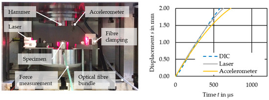
Figure 5.
Measurement of the hammer displacement.
For the shadowing method, a light beam shines orthogonal to the displacement direction of the observed object and received by a photoelectric element. During the measurement, the observed object moves into the light beam causing a partial shading effect, which leads to changes in the electrical measurement signal. This method was successfully applied to analyze high-speed forming processes in [51] and more recently in [52]. Here, a laser (wavelength 650 nm, power 16 mW) with line optics and a photoelectric receiver circuit consisting of a position sensitive device (PSD) as a photoelectric receiver element and an electronic amplifier were used together with a suitable current source. Static tests of the system have proved good accuracy with a mean deviation of 0.05 mm and 2.1%, respectively, and a maximum deviation of 0.15 mm or 10% for a measuring range of 4 mm. To determine the hammer displacement by means of DIC, the process was recorded with a high-speed camera (FASTCAM SA4, Photron), and then the displacement of the hammer or the specimen was digitally evaluated with ARAMIS Professional 2017 (facet size = 11 pixels, dot pitch = 5 pixels).
Figure 6 shows 4 of about 30 images of an exemplary image sequence taken during a shear test with a frame rate of 30.000 fps and a resolution of 384 × 288 pixels. Here, the shift of marked facet point 1 corresponds to the displacement of the hammer shown in Figure 5. A facet outside the deformation range of the shear tensile test (facet point 2) serves as a comparison point.
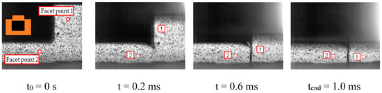
Figure 6.
Image sequence for DIC taken during a shear test.
Table 2 compares calculated and measured process variables for the setup with a pneumatically driven hammer for an initial filling pressure of 0.7 MPa. While the measured pressures agree very well with the calculated values, correcting the analytically determined acceleration is necessary because frictional forces due to sealing elements reduce the acceleration (see Equation (4)).
Table 2.
Calculated and measured parameter values for the setup with a pneumatically driven hammer.
2.2.2. Experimental Setup Using Electromagnetically Driven Tools
Numerical simulation assisted the design of the electromagnetically driven acceleration unit in order to make sure that forming speeds of the order of magnitude up to105/s are achievable in the specimen. As shown in Figure 7, the test setup consists of the electromagnetically driven acceleration unit, the actual hammer, the specimen holder, the measuring body for measuring the effective loads and the housing.
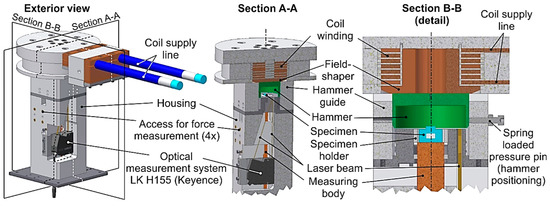
Figure 7.
Design of the experimental setup with electromagnetically driven tools.
The acceleration unit consists of a cylindrical coil with a fieldshaper, which is suitable for converting the predominantly radially directed force in a cylindrical coil into a force acting predominantly axially on the hammer. For the experiment, the coil is connected to a pulsed power generator; the capacitor of the pulsed power generator is charged to a defined voltage and then discharged through the tool coil to provide a damped sinusoidal current. This time-dependent current induces a magnetic field, which in turn causes an oppositely directed current in the fieldshaper, as shown in Figure 8. Due to the special fieldshaper geometry, the arrangement of coil winding, fieldshaper and hammer and the skin effect, a current flowing at the surface facing the hammer closes the current loop in the field shaper. This induces a magnetic field in the gap between field shaper and hammer and an oppositely directed current in the hammer at the surface facing the fieldshaper. The interactions between the magnetic fields and the currents cause Lorentz forces in fieldshaper, coil winding and hammer, which can be converted into a so-called magnetic pressure. Finally, the forces between field shaper and hammer cause the acceleration of the hammer in the direction away from the field shaper (i.e., downwards in Figure 8).
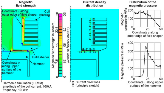
Figure 8.
Magnetic field strength, current density, and magnetic pressure in the electromagnetically driven acceleration unit.
Compared to conventional (i.e., usually spiral) flat coils, the setup with cylindrical coil and fieldshaper offers the possibility of using more coil turns with the same diameter of the pressurized circular area, resulting in a higher inductance of the inductor unit (consisting of coil and fieldshaper) thus leading to a longer power pulse. Consequently, the transformation of the capacitor charging energy into kinetic energy of the hammer is more effective. In addition, the coil load is less critical compared to a spiral coil. Since the latter is usually used directly (that is, without field shaper) the deformation of the workpiece in case of electromagnetic sheet metal forming or the displacement of the hammer in case of processes with electromagnetically accelerated tools leads to significant changes in the direction of loading. Frequently unfavorable load conditions for the coil, especially in case of slow current and force pulses accompany these changes [52]. This may significantly reduce coil life. In addition, the force distribution acting on the hammer is more homogeneous than in case of spiral coils and there are fewer transverse forces, which can cause tilting of the hammer in the guide.
The hammer design aims at obtaining high dynamics via consistent weight reduction and avoiding a deformation of the hammer due to the impulsive and inhomogeneous Lorentz force distribution at the same time. In addition, an adequately long guide length is necessary in order to avoid tilting of the hammer in the guidance during the flight. Due to the complex set of requirements, numerical investigations assisted the design process. First, the movement and deformation of cylindrical hammers were calculated as a function of the material (aluminum and steel), the geometry parameters diameter and height, and the process parameter capacitor charging energy. The coupled electromagnetic and mechanical simulation considered the characteristics of the pulsed power generator PS 103-25 Blue Wave by PSTproducts available at the Fraunhofer IWU as input data (see Table 3).
Table 3.
Characteristics of the pulsed power generator PS 103-25 Blue Wave available at Fraunhofer IWU.
Simulations proved that, as expected, the hammer speed increases with increasing capacitor charging energy (see Figure 9). At the same time, a more pronounced oscillation of the hammer occurs. With increasing hammer mass, the conversion of capacitor charging energy into kinetic energy of the hammer is less efficient, while the vibrational behavior tends to be unaffected by this parameter. As a result, aluminum hammers achieve higher kinetic energies and much higher speeds than steel hammers with the same parameters.
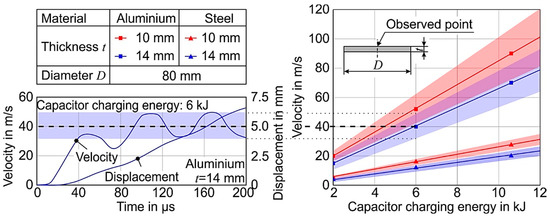
Figure 9.
Velocities of electromagnetically accelerated hammers.
Therefore, an aluminum hammer with a diameter of 100 mm was used in the final design of the test rig. To realize a sufficient guide length (35 mm) at low mass the hammer was designed as a solid cylinder with a length of 15 mm followed by a hollow cylinder with 3.5 mm wall thickness and a length of 20 mm (see Figure 7 and Figure 8). To avoid lateral forces and moments due to the weight, the direction of movement of the hammer is oriented vertically downwards. At the beginning of the process, spring-loaded pressure pins hold the hammer in position and ensure a small gap between field shaper and hammer. During the process, the measurement system Keyence LK-H155, which bases on laser triangulation with a maximum sampling rate of 392 kHz, records the displacement of the hammer.
The sample holder serves for the exact positioning of the specimen in the test setup and prevents buckling of the laminated sheet specimens during the test. To reduce the frictional forces between the specimen and the specimen holder and to avoid that they distort the force measurement, the specimen holder is made of polyoxymethylene (POM). Numerical sensitivity analyses supported the estimation of the influence of the gap between the specimen and the specimen holder on the force measured on the measuring body. They show no noteworthy change of the measuring signal for gap widths of 0.05 mm to 0.2 mm, whereas for a theoretical zero gap, the force signal is significantly higher. Thus, a gap of 0.1 mm was chosen for the experimental realization.
Strain gage-based force measurement quantified the acting loads during the process. Application of the strain gage to the specimen itself is hardly possible because of its small size. Therefore, a suitable measuring body was implemented in the test setup. Two symmetric half bridges were applied 30 mm from the top and 8 mm from the side of the measurement body. This brings the additional advantage that after installing and calibrating the system once, it is available for numerous tests, while strain measurement directly on the specimen necessitates preparation of each single specimen. However, the design of the measuring body must provide for different requirements. Specifically, it must guarantee that the detected strains are high enough to produce a clearly measurable signal (high sensitivity), but still avoid any plastic deformation. Moreover, due to the highly dynamic process, neither the specimen nor the measuring body is loaded homogeneously, but the transient force and the corresponding strain travel as a wave through the setup. Interferences of the original signal and the reflected signal complicate the interpretation of the measurement signal to impossibility. Even using inverse simulation strategies for the interpretation of the test results cannot solve this problem, because the solution is not unique. Therefore, the design of the measuring body must guarantee that interference occurs only after detection of the complete load signal. Therefore, bar-shaped measuring bodies of sufficient length are most suitable. The minimum distance x between the measurement point and the end of the measuring body depends on the duration of the test Δt (from the moment of force initiation tini until the moment of failure tfail of the specimen) and the sonic velocity csonic in the material (here steel). The latter in turn depends on the Young’s modulus E and the density ρ of the material (see Equation (7)).
To estimate the duration of the experiment, exemplary shear tests were numerically simulated using a flow curve determined for DC06 under quasistatic loading. Additional simulations using strain rate dependent flow curves from high-velocity tensile tests and different strains at failure served for the verification of the sensitivity of the measurement result against the material and failure characteristics. Figure 10 shows that the strain-time curve clearly reflects differences in both the yield stress and the failure strain. Furthermore, a duration of the test of up to approx. 60 μs results for the shear sample from DC06. This corresponds to a minimum distance of at least 175 mm between the measuring point and measuring body end.
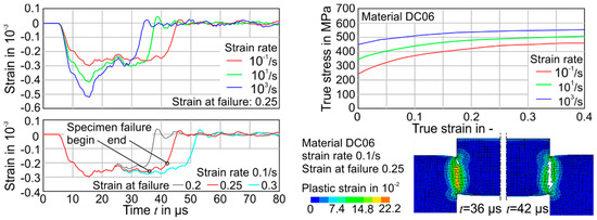
Figure 10.
Sensitivity of the strain signal to yield stress and failure strain.
With the aim of eliminating the reflection of the measuring signal at the end of the measuring body by sophisticated use of interferences, thus reducing the measuring body length, different measuring body geometries and the corresponding influences on the resulting strain signal were analyzed numerically.
The calculations show that an accumulation of mass at the end of the measuring body and a sophisticated geometry is indeed suitable for significantly reducing the amplitude of the resulting measuring signal, but complete extinction was not possible for the investigated geometries (see Figure 11).
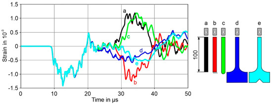
Figure 11.
Influence of different measuring body geometries and boundary conditions on the resulting strain signal (mid, 10 mm from the upper end) for an impact test to the steel measurement body.
To allow reliable measurement of other specimen shapes and materials, too, a measuring body with a length of 720 mm and a cross section of 6 mm × 35 mm was implemented in the test setup. This is suitable for test periods up to approx. 200 μs. Quasi-static tests of the measuring system demonstrated its principal functionality. For this purpose, the test setup including the measuring system was subject to mechanical loading in a manual press. Figure 12 shows that the force-displacement curves detected via the strain gauge-based system are in good agreement with similar curves detected by a commercial piezo-based force-measuring ring during the same experiment. The reason for the small drops in force, clearly detectable in the curves belonging to the shear tests, is the manual operation of the press.
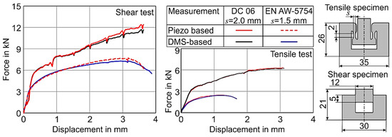
Figure 12.
Quasi-static testing of the load measurement system, which also serves for calibration of the Youngs-modulus of the measurement body made of C45E.
The housing of the setup is mostly made of plastic. It serves for the relative positioning of the specimen, displacement-measuring system, and the described essential components of the experimental setup.
2.3. Inverse Identification of Material Parameters
Figure 13 shows the procedure for determining the hardening and damage parameters for material modeling in numerical simulations. It starts with the conventional quasi-static tests for different stress states (box I in Figure 13). These provide input data for the selected material model (box II in Figure 13) and serve for the full identification of the plasticity at quasi-static loading (box III in Figure 13). This is the starting point for the optimization that aims at the determination of strain rate dependence and failure strain at high speeds. For the latter, high-speed experiments are carried out using the experimental test setups developed above (box IV in Figure 13), and separate non-coupled optimizations for the different specimen geometries are performed using LS-OPT by LSTC (box V in Figure 13). On this basis, the strain rate dependent parameter c and the strains at failure are identified for the respective stress states (box VI in Figure 13).
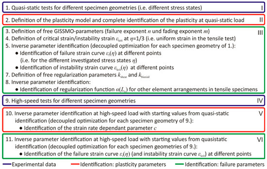
Figure 13.
Procedure for identification of the material model.
The design variable in the optimization with LS-OPT is the distance of characteristic points on the simulated curves to the experimental data. In contrast to target function variables based on the mean square error or a curve mapping, these target variables are relatively simple and allow disregarding potential curve artifacts. However, the application requires that the simulated curves are in good agreement with the experiment and the influence of design variables is limited to shifts of curve areas in x- or y- direction. The regarded case complies with these requirements.
For the material modeling, the quasi-static yield stress is multiplied by a factor , which describes the strain rate dependence, and by a factor describing the damage (see Equation (8)). Equation (10) approximates the deformation rate dependency of the materials logarithmically and Equation (11) using an exponential approach, both with limitations for low strain rates. The factor c is the multiplier of the logarithm pattern known from the Johnson-Cook-Model. Typically, this leads to a linear curve of the flow stress scaling in a logarithmic plotting over the strain rate. In contrast, the exponential approach of the flow stress scaling valuates higher strain rates with a higher scaling. The damage description bases on the GISSMO model (see Equation (9)) using the typical Lemaitre approach for stress reduction in the yield locus. Here, the stress triaxiality η plays a key role [53].
3. Results
3.1. Quasi-Static Material Characterization and Modeling
Following the described strategy for the identification of material parameters, an extensive quasi-static characterization of the material was carried out first, considering tensile specimens, notched tensile specimens and two different shear tensile specimens. Due to the limitation of the Barlat 2000 model [54] to shell models with a plane stress state, von Mises plasticity was assumed. The modeling assumes isotropic hardening and uses the phenomenological GISSMO damage model [53] for describing the failure. The latter requires the definition of the failure strain curve εf(η), the instability strain curve εkrit(η), the free GISSMO parameters damage exponent n and the fading exponent m, the regularization function α(Le) and the free regularization parameters kshear and kbiax. Figure 14 shows the identified quasi-static characteristics and curves for DC06.
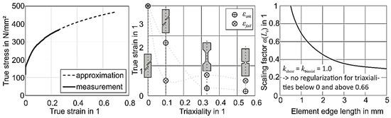
Figure 14.
Results of the quasistatic analysis of DC06. Left: Flow curve. Middle: Failure strain and critical strain (starting of damage) of the GISSMO model. Right: Determined regularization curve.
Internal investigations have shown that the damage exponent and the fading exponent are equally sensitive to the identified sizes of failure strain and critical strain. According to commonly accepted assumptions, the development law of damage D follows a quadratic development so that the damage exponent and the fading exponent were fixed as 2.0. An inverse characteristic determination with LS-OPT provided the four points of the failure strain curve (from four specimen geometries with different stress states) and the three unknown points of the critical strain curve (the value of εcrit of the flat tensile specimen corresponds to the uniform elongation and was available directly from the experimental data). Considering the tensile test as an example, inverse parameter identifications with different element sizes served for determining the regularization function α (see Figure 14, right).
3.2. Material Characterization and Modeling at High Strain Rates
3.2.1. Experimental Tests
In the next step, load and resulting deformation of the specimen were recorded in high-speed experiments. Measurement curves of multiple tests were averaged and the resulting curves were smoothed and filtered in order to serve as input data for the optimization calculation. Figure 15 shows exemplary results for the pneumatically driven setup and DC06 specimens, and Figure 16 illustrates corresponding curves for the electromagnetically driven setup with a hammer velocity of approximately 30 m/s.
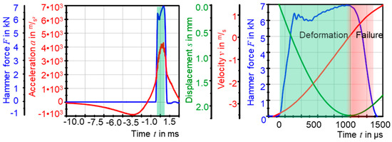
Figure 15.
Deformation and load course measured on the pneumatically driven setup.
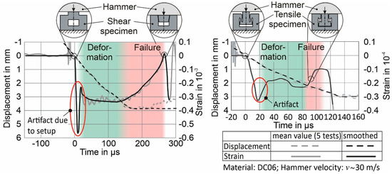
Figure 16.
Hammer displacement and load course (elastic strain of the measurement body) measured on the electromagnetically driven setup for a hammer velocity of approximately 30 m/s. The curves shown here have been measured with a 6 mm thick measurement body.
It is obvious that the strong increase of load characterizing signal—i.e., the force measurement in case of the pneumatically accelerated system and the force-equivalent strain signal in case of the electromagnetically driven setup—indicates the impact of the hammer on the specimen. The characteristic peak at the impact, which is more distinct in case of the electromagnetically driven hammer, is an artifact due to the setup and therefore it is disregarded in the inverse parameter identification. After the impact, the signal remains relatively constant between 6 kN and 7 kN for the exemplary curves recorded for the pneumatically driven setup, and at force-equivalent strain levels of approximately 3.3 × 10⁻³ for the exemplary shear test and approximately 2.0 × 10⁻³ for the exemplary tensile test performed using the electromagnetically driven setup. This section of the curve describes the deformation of the specimen and serves as input data for the inverse identification of the Johnson Cook parameters describing the plastic material flow. The subsequent decrease in the force signal and the force-equivalent strain signal, respectively characterize the failure of the specimen. This section of the curve serves as input data for the inverse identification of the failure parameters. In the force-equivalent strain curves measured for the electromagnetically driven setup, the hammer finally bounces on the shoulder, which causes a significant increase in force. This serves to control the measurements, but it is irrelevant for the optimization calculations leading to the material parameters.
3.2.2. Inverse Parameter Identification
Figure 17 compares measured force-equivalent strain curves for specimens made of DC06 and EN-AW5754 H111 with corresponding numerically determined ones. The deformation rate parameter c and the failure strain εfail were identified. The diagram areas that characterize the specimen deformation (highlighted in green) were used to determine the strain rate dependence and areas that characterize the failure (highlighted in red) were used to identify the damage parameters. Neglecting the artifact pulse generated after the impact of the flyer results in a good agreement of the numerically and experimentally determined curves.
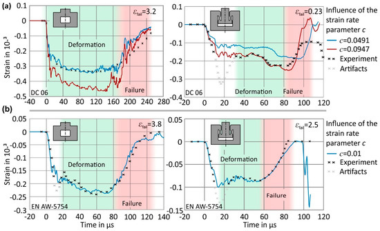
Figure 17.
Comparison of experimentally and numerically determined elastic strain-time curves on the measuring body for shear and tensile specimens of DC06 (a) and EN-AW5754 H111 (b) at a hammer velocity of approximately 30 m/s.
As expected, the elongation at failure differs significantly depending on the dominant stress state in the sample. In the example shown, the value determined for the tensile test specimen (DC06 εfail = 0.23, AW5754 εfail = 2.5) is significantly lower than the one determined for the shear test (DC06 εfail = 3.2, AW5754 εfail = 3.8). Similarly, for DC06, the determined strain rate dependency differs as a function of the dominant stress state in the specimen. The deformation rate parameter for the DC06 determined in the shear test (identified c = 0.0491 or m = 0.038) is significantly lower than for the tensile test (identified c = 0.0947 or m = 0.063). To illustrate the deviation, Figure 17 also shows the curves that result from the deformation rate parameter identified in the respectively other test (shear vs. tension). As expected, the material AW5754 H111 feature significantly lower strain rate sensitivity and in contrast to DC06 there is no difference in the identified rate parameter (c = 0.01 or m = 0.016) depending on the stress state.
A critical comparison of numerically and experimentally determined curves (Figure 17) shows that especially for the material DC06 the decrease of the force-equivalent strain on the measuring body due to specimen failure or damage occurring in the experiment is flatter than in the simulation. There are several possible causes for this, which in combination lead to the extent shown in Figure 17. The presented curves contain information from five experiments each with four tested specimens and two test areas per specimen (40 test areas). Even slight time deviations at the time of failure of the individual test areas blur the steep drop in the course of the curve. In addition, the shearing samples do not completely fail in the middle of the shear zone (see Figure 1). However, a drop in the strain signal is clearly visible due to the significantly reduced cross section in the test area. The model is not fully capable of simulating this shear failure, and an additional influence exists caused by the friction in the failed shear zone, the element size in the simulation (in the test area about 0.15 mm), and the assumed yield stress at large plastic strains. The latter is available from the uniaxial tensile test only up to 0.26 and was extrapolated to strains of three, resulting in possible deviation in the extrapolated range.
The determined material and failure characteristics can be assigned directly to a hammer speed, but the same hammer speed produces significantly different deformation rates and distributions for different specimen geometries. Figure 18 exemplarily shows a typical distribution of the strain rates resulting from a hammer velocity of approx. 30 m/s for shear specimens and tensile specimens made of DC06.
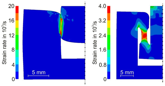
Figure 18.
Distribution of the strain rate in DC06 shear and tensile specimens at the moment of maximum strain rate for a hammer velocity of 30 m/s.
The maximum strain rates in the test area of the shear test range from approx. 15 × 103/s up to 30 × 103/s, while in the test area of the tensile specimens’ strain rates of approx. 3.5 × 10³/s up to 5.5 × 10³/s occur. In addition, there is a strong time dependency of the strain rate. Therefore, a defined assignment of the flow curves to a single strain rate is meaningless, as with all high-speed operations. However, in the context of the inverse parameter identification considering all relevant parts of the test setup, time- and position dependent inhomogeneities of strain or strain rate are completely taken into account.
Figure 19 shows the identified GISSMO parameters describing the failure and damage of the material, the flow stress scaling for both discussed strain rate sensitivity approaches, and finally the flow curves, which could be, generates for arbitrary strain rates from the identified model. However, these generated flow curves are solely robust and reliable for the investigated range of strain rates (i.e., 4 × 10³/s up to 25 × 103/s for the electromagnetic accelerated test setup).
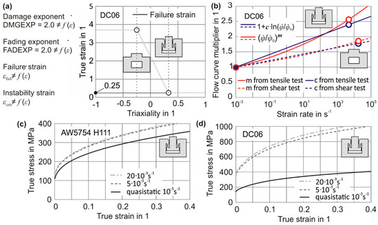
Figure 19.
(a) Identified GISSMO parameters for DC06. (b) Identified strain rate sensitivity of DC06 for the two investigated models. (c) Flow curves of AW5754 H111 generated from the identified model for different strain rates show no significant forming velocity dependency. (d) Flow curves of DC06 generated from the identified model for different strain rates show a high strain rate dependency.
In fact, the flow curve multiplier, i.e., the over stress due to strain rate sensitivity, was identified slightly different for the two approaches (see Figure 19b) at the tested strain rate working points. The reason for this is the nonhomogeneous strain rate distribution inside the specimen. The GISSMO model allows the input of failure strain and critical strain curves for different strain rates, which is necessary for a practical application because of the significant differences between high-speed and quasi-static investigations. It is obvious that in the high extrapolation range the strain rate dependency is underestimated if the logarithmic approach is applied compared to the exponential approach (Figure 19b). Hence, for high-speed applications a double logarithmic approach or the exponential approach is recommended as experiments for different strain rates indicate [33].
4. Discussion
4.1. Sensitivity Study
A sensitivity analysis served for assessing the suitability of the test setup and the accuracy of the identified material and failure parameters. Figure 20 shows that even slight changes of the rate parameter c and the failure strain εfail lead to significantly changed courses of the time-dependent force-equivalent strain curves. This high sensitivity of the measurement curves to the relevant material parameters suggests that the characteristic of the test setup is applicable for a sufficiently accurate and trustworthy inverse parameter identification. In particular, the flow stress increase, i.e., a high strain rate sensitivity, is obvious for the material DC06 as the curve for a disregarded strain rate dependency (c = 0.0) in Figure 20 reveals due to a quite different strain level at the measurement body. High strain rate sensitivities of the DC steel grades have been also found e.g., in [55,56].
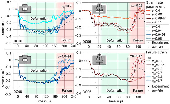
Figure 20.
Sensitivity of the simulated strain-time curves at the measurement body of the electromagnetically accelerated test setup. Investigated material DC06 regarding the rate parameter c and the strain at failure at a nominal hammer speed of approximately 30 m/s.
4.2. Verification of the Identified Material Parameters
To evaluate the determined material parameters further, reference tests according to the principle of free electromagnetic sheet metal forming were carried out for verification purposes. This means that the coil housing and a drawing ring clamp the sheet metal between each other, but there is no additional die restricting the forming process or influencing the resulting shape of the part. This eliminates disturbances such as friction, which add unnecessary uncertainties to the simulation model, and allows focusing on material related parameters identified above. This process variant successfully served for verifying and evaluating the numerical simulation e.g., in [57].
The same coil system serving for the electromagnetic acceleration in the high-speed material testing device described in Section 2.2.2 was used in these verification experiments. The used drawing ring has a diameter of 100 mm and a drawing radius of 5 mm. During the deformation process, the measurement system Keyence LK-H155 records the workpiece deformation in the center of the component. Only at this point does the laser beam of the optical measuring technology hit the workpiece surface perpendicularly during the entire forming process, which is a boundary condition required for the measuring principle. Literature proves that the deformation of the component is purely inertia-driven (no Lorentz forces act on the workpiece) and starts relatively late in the process in this area, while the areas in the immediate vicinity of the field shaper, and in particular in the area of the middle radius, are accelerated earlier [52]. However, this is no obstacle for the basic verification of the material characteristics. This region can even be considered particularly suitable since the highest velocities occur in this area and the strain rate dependence of the material behavior should therefore be particularly pronounced here. In addition to the displacement measurement, a probe based on the principle of voltage induction in a Rogowski coil (precisely a CWT 1500/4/1000 by Power Electronic Measurement—PEM) recorded the time course of the coil current [58]. For the experiments, a test stand was designed and implemented, which allows reproducible positioning of the tool coil including the fieldshaper, the workpiece, the drawing ring and the position measuring system (see Figure 21a).
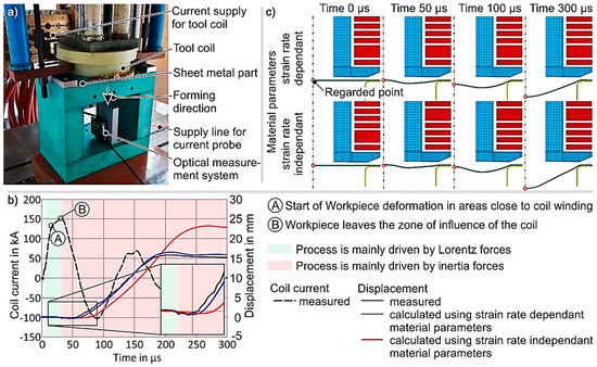
Figure 21.
Verification of the identified material parameters of DC06: (a) test setup, (b) current course and comparison of experimentally and numerically determined displacement courses, (c) numerically determined forming stages.
Using this test stand and applying different capacitor charging energies, components were formed from the same sheet metal material considered in the material characterization presented above. Figure 21b exemplarily shows measurement results of a forming operation at a capacitor charging energy of 5 kJ. As expected, the coil current features a damped sinusoidal profile. The bending of the curve at point A is due to an inductance change, which indicates the beginning of the workpiece deformation. From point B on, the curve is sinusoidal again. Thus, it can be assumed that the workpiece left the area of influence by the coil and the further deformation no longer has a significant effect on the total inductance of the unit consisting of coil, fieldshaper and workpiece. From then on, the process is purely inertia-driven [52].
The measured current profile served as input data set to characterize the effective loads in the process simulation, which was carried out as a coupled electromagnetic and structural mechanical simulation in LS-Dyna. In addition to the mechanical characteristics identified in AP4, material modeling also requires knowledge of electrical conductivity. For this reason, the conductivity of sheet metal strips (width: 10 mm, thickness: 1 mm, length: 1000 mm, distance between measuring points: 800 mm) was determined via the four-wire sensing. For DC06 a conductivity of 8.5 MS/m was determined, which corresponds to typical values.
To verify the material characteristics, Figure 21b compares numerically calculated displacement-time curves to the measured one. The numerical results include both material parameters identified via inverse simulation of the high-speed material test as well as material parameters determined for quasi-static loads. In addition to the displacement-time curves Figure 21c shows forming stages at significant times during the process in order to give an overview of the deformation behavior of the entire component.
As the coil current increases a half toroidal deformation of the component occurs when the yield stress is reached, while the center of the component still shows no significant displacement. After 25 μs, the component surface in the center of the specimen is first slightly deflected in the negative direction of measurement (that is, toward the coil). The higher-resolution detail section of the diagram in Figure 21b shows this deflection for the measurement curve as well as for both simulation curves. The effect is due to a bending deformation in this area caused by the deformation of the component in the areas close to the fieldshaper. From approx. 55 μs, the displacement increases significantly, reaches its maximum value (15.6 mm) within approx. 145 μs and then oscillates at approx. 15.1 mm. The simulation with strain rate dependent material parameters agrees very well with the experiment. The deviation in the increase of up to 4 μs lies within the repetition accuracy of the measurement. The deviation of approx. 0.9 mm in the achieved displacement corresponds to less than 6% of the value. In addition, considering the slope of the curve, i.e., regarding the displacement speeds, the deviation lies within the measurement accuracy. The result of the simulation with quasistatic material parameters diverges much more from the experiment. Although the curve in Figure 21b still looks quite similar, the deviation considering the displacement velocity is more than 11%. The increase in the displacement-time curve occurs with a delay of approximately 20 μs compared to the experiment, since for a softer material the toroidal forming stages are more pronounced before the center region of the specimen follows (see Figure 21c). The simulation overestimates the displacement by approx. 50% at 22.7 mm. This clearly shows that the strain rate-dependent material properties lead to significantly better accuracy of the numerical process simulation. The strong influence of strain rate sensitivity on forming was also numerically proven by Figueiredo et al. [59]. The remaining small deviations may be due to inaccuracies in the modeling. For example, errors of the order of magnitude of a few tenths of a millimeter cannot be ruled out in the modeling of the gap width between workpiece and field shaper. Furthermore, the temperature was neglected in the simulation, although at least for a short time a warming is to be expected due to the resistive losses and the deformation. The increased temperature can lead to the formation of so-called adiabatic shear bands, which locally influence the material behavior [60]. Winter et al. [61] were able to show in finite element simulations without thermal coupling that the occurring microstructural effects could nevertheless be well described.
5. Conclusions and Outlook
A method for the determining material characteristics in processes with high forming speeds was successfully developed. Then it was demonstrated by verification tests based on the principle of free electromagnetic forming that the application of this method allows numerical modeling of high-speed processes with good accuracy. The material parameters determined for steel DC06 show clear differences for different stress states. It is remarkable that not only the strain at failure but also the strain rate dependency seems to be a function of the stress state. Precisely, nearly twice as high yield stresses were determined for specimen geometries with predominantly uniaxial tensile load at forming speeds of the order of 105 s−1 as compared to shear tests for DC06. This effect does not occur under quasi-static loading and contradicts - at first sight - the widespread continuum mechanical assumption of an isotropic widening of the yield surface for the strain rate dependency. However, it coincides with findings on the anisotropy of the strain rate dependency for different stress states of Lenzen et al. [62]. By contrast, for the aluminum alloy EN-AW5754-H111 the rate hardening behavior is less significant and independent of the stress state.
One possible explanation for the apparently triaxiality-dependent strain rate dependency of the DC06 material is that simulation disregarded the heating. At high strain rates and correspondingly short process times forming processes can be considered quasi-adiabatic, because the heat generated during forming cannot dissipate fast enough. Consequently, the temperature in the forming zone rises and thus, thermal softening effects superpose the strain hardening. Especially in case of small deformation zones and for materials with limited thermal conductivity this can lead to an autocatalytic localization of the forming area [63]. In high-speed cutting processes, so-called shear bands indicate this effect in the microstructure of the material. First micrographic investigations have revealed a distinct shear band in the DC06 shear specimen. In case of the tensile specimen forming is not as localized as in the shear specimen and therefore the temperatures in the specimen can be expected to be lower leading to less significant thermal softening. For the EN-AW 5754 H111 however, the strength is lower and the thermal conductivity is higher than for DC06. Therefore, there are fewer heat results for both specimen geometries, so that the mentioned autocatalytic localization does not occur.
Taking into account adiabatic warming in the inverse simulation might help to investigate these results in more detail and to develop the determination of material parameters further. Separating the effects will fundamentally explore whether the stress state actually influences the strain rate dependent velocity dependence of DC06 or whether it is a fictitious dependence, which is entirely due to a superimposed temperature effect, caused by different adiabatic warming due to different strain distributions.
Author Contributions
Conceptualization, V.P., C.S. and A.B.; Formal analysis, V.P., C.S. and M.T.; Funding acquisition, V.P., C.S. and A.B.; Investigation, C.S., M.T. and S.W.; Methodology, C.S. and M.T.; Project administration, V.P., C.G. and A.B.; Resources, A.B.; Software, C.S. and M.T.; Supervision, V.P. and A.B.; Validation, V.P. and C.S.; Visualization, V.P., C.S. and M.T.; Writing—original draft, V.P., C.S., M.T. and S.W.; Writing—review & editing, V.P., C.G. and A.B. All authors have read and agreed to the published version of the manuscript.
Funding
This research was funded by the Deutsche Forschungsgemeinschaft (DFG, German Research Foundation), grant number PS 68/2-1 and BR 3500/18-1.
Conflicts of Interest
The authors declare no conflict of interest. The funders had no role in the design of the study; in the collection, analyses, or interpretation of data; in the writing of the manuscript, or in the decision to publish the results.
References
- Neugebauer, R.; Bouzakis, K.D.; Denkena, B.; Klocke, F.; Sterzing, A.; Tekkaya und, A.E.; Wertheim, R. Velocity effects in metal forming and machining processes. CIRP-Ann. Manuf. Technol. 2011, 60, 627–650. [Google Scholar] [CrossRef]
- Psyk, V.; Linnemann, M.; Sebastiani, G. Electromagnetic pulse forming. In Mechanics of Materials in Modern Manufacturing Methods and Processing Techniques; Elsevier: Amsterdam, The Netherlands, 2020. [Google Scholar]
- Lange, K.; Müller, H.; Zeller, R.; Herlan, T.H.; Schmidt, V. Hochleistungs-, Hochenergie-, Hochgeschwindigkeitsumformen. In Umformtechnik—Sonderverfahren, Band 4; Springer: Berlin, Germany, 1993; pp. 7–46. [Google Scholar]
- Schüßler, M. Hochgeschwindigkeits-Scherschneiden im Geschlossenen Schnitt zur Verbesserung der Schnitteilequalität. Ph.D. Thesis, Technische Hochschule, Darmstadt, Germany, 1990. [Google Scholar]
- Bruno, E.J. High-Velocity Forming of Metals; American Society of Tool and Manufacturing Engineers: Daerborn, MI, USA, 1968. [Google Scholar]
- Wielage und, H.; Vollertsen, F. Classification of Laser Shock Forming within the Field of High Speed Forming Processes. J. Mater. Proc. Technol. 2011, 211, 953–957. [Google Scholar] [CrossRef]
- Psyk, V.; Risch, D.; Kinsey, B.L.; Tekkaya, A.E. Electromagnetic Forming—A Review. J. Mater. Proc. Technol. 2011, 211, 787–829. [Google Scholar] [CrossRef]
- Neugebauer, R.; Bräunlich, H.; Kräusel, V. Umformen und Schneiden mit Hochgeschwindigkeit—Impuls für die ressourceneffiziente Karosserieteilbearbeitung. In 5. Chemnitzer Karosseriekolloquium—Karosseriefertigung im Spannungsfeld von Globalisierung, Kosteneffizienz und Emissionsschutz; Fraunhofer-Institut für Werkzeugmaschinen und Umformtechnik: Chemnitz, Germany, 2008. [Google Scholar]
- Tobias, S.A. Survey of the development of petro-forge forming machines. Int. J. Mach. Tool Design Res. 1985, 25, 105–197. [Google Scholar] [CrossRef]
- Risch, D. Energietransfer und Analysse der Einflussparameter der Formgebundenen Elektromagnetischen Umformung; Shaker: Aachen, Germany, 2009. [Google Scholar]
- Uhlmann und, E.; Scholz, M. Zerteilen von Aluminiumblechen durch Impulsmagnetfelder. In 2. Kolloquium Elektromagnetische Umformung; Technische Universität Dortmund: Dortmund, Germany, 2003. [Google Scholar]
- Marré, M.; Beerwald, C.; Psyk, V. Einfluss der Geschwindigkeit beim kraftschlüssigen Fügen rohrförmiger Werkstücke durch elektromagnetische Kompression. In 11. Paderborner Fügesymposium, Mechanisches Fügen und Kleben; Universität Paderborn: Paderborn, Germany, 2004. [Google Scholar]
- Weddeling, C.; Woodward, S.; Marré, M.; Nellesen, J.; Psyk, V.; Tekkaya, A.E. Influence of groove characteristics on strength of form-fit joints. J. Mat. Proc. Technol. 2011, 211, 925–935. [Google Scholar] [CrossRef]
- Psyk, V.; Scheffler, C.; Linnemann, M.; Landgrebe, D. Process analysis for magnetic pulse welding of similar and dissimilar material sheet metal joints. Pro. Eng. 2017, 207, 353–358. [Google Scholar] [CrossRef]
- Vohnout, V. A Hybrid Quasi-Static/Dynamic Process for Forming Large Sheet Metal Parts from Aluminum Alloys; Ohio State University: Columbus, OH, USA, 1998. [Google Scholar]
- Jäger, A.; Risch und, D.; Tekkaya, A.E. Verfahren und Vorrichtung zum Strangpressen und nachfolgender elektromagnetischer Umformung. Patent DE 10 2009 039 759.0, 30 April 2009. [Google Scholar]
- Golovashchenko, S.F. Springback Calibration Using Pulsed Electromagnetic Field. AIP Conf. Proc. 2005, 778, 284–285. [Google Scholar]
- Psyk, V. Prozesskette Krümmen—Elektromagnetisch Komprimieren—Innenhochdruckumformen für Rohre und Profilförmige Bauteile; Shaker: Aachen, Germany, 2009. [Google Scholar]
- Breitling, J. The Challenges and Benefits of High-Speed-Blanking; DGM Informationsgesellschaft mbH: Frankfurt, Germany, 1998. [Google Scholar]
- Chanin, M.; Koskoris, J. Dynapak 1-1/2 Million Foot Pound Forging Machine; Defense Technical Information Center: Alexandria, VA, USA, 1969. [Google Scholar]
- Neugebauer, R.; Kräusel, V.; Weigel, P. Effekte des adiabatischen Trennens im Vergleich zum konventionellen Scherschneiden. Stahl und Eisen 2010, 130, 39–42. [Google Scholar]
- Uhlmann, E.; König, C.; Ziefle, A.; Prasol, L. Coining of Micro Structures with an Electromagnetically Driven Tool. In Proceedings of the 5th International Conference on High Speed Forming—ICHSF, Dortmund, Germany, 24–26 April 2012. [Google Scholar]
- Vitvaz und, P.A.; Davies, R. Uses of the Petro-Forge high-speed machines in powder metallurgy. Powder Metall Met. Ceram. 1975, 14, 343–345. [Google Scholar]
- Yaldiz, S.; Saglam, H.; Ünsacar, F.; Isik, H. Design and application of a pneumatic accelerator for high speed punching. Mater. Desig 2007, 28, 889–896. [Google Scholar] [CrossRef]
- Taber, G.; Kabert, B.A.; Washburn, A.T.; Windholtz, T.N.; Slone, C.E.; Boos, K.N.; Daehn, G.S. An Electromagnetically Driven Metalworking Press. In Proceedings of the 5th International Conference on High Speed Forming—ICHSF, Dortmund, Germany, 24–26 April 2012. [Google Scholar]
- High-Speed Testing Machines from 25 to 160 kN. Available online: https://www.zwickroell.com/en/servohydraulic-testing-machines/high-speed-testing-machine (accessed on 19 June 2019).
- Biermann, H.; Krüger, L. Moderne Methoden der Werkstoffprüfung; WILEY-VCH: Weinheim, Germany, 2015. [Google Scholar]
- Abouridane, M. Bruchverhalten von Leichtmetallen unter Impact Beanspruchung; Technische Hochschule Aachen: Aachen, Germany, 2005. [Google Scholar]
- Kleiner, M.; Tekkaya, A.E.; Demir, K.; Risch, D.; Psyk, V. A drop-weight high-speed tensile testing instrument. Prod. Eng. 2009, 3, 75–180. [Google Scholar] [CrossRef]
- Walley, S.M.; Field, J.E.; Proud, W.G. A review of the Techniques available of Obtaining the Mechanical Properties of Materials at High Rates of Strain. In Proceedings of the 1st International Conference of High Speed Forming—ICHSF, Dortmund, Germany, March 31–April 1 2004. [Google Scholar]
- Homayun, M. Verhalten Mechanischer Werkstoffe im Bereich hoher Verformungsgeschwindigkeiten; Technische Hochschule Aachen: Aachen, Germany, 1987. [Google Scholar]
- Rotationsschlagwerke. Available online: https://www.nordmetall.net/de/rotationsschlagwerke/ (accessed on 19 June 2019).
- Halle, T. Zusammenhänge Zwischen Spanvorgängen und dem mechanischen Werkstoffverhalten bei hohen Dehnungsgeschwindigkeiten. Ph.D. Thesis, Technische Universität Chemnitz, Chemnitz, Germany, 2005. [Google Scholar]
- Hopkinson, B. Method of Measuring the Pressure Produced in the Detonation of High Explosives or by the Impact of Bullets. Philos. Trans. Royal Soc. London Ser. A 1914, 213, 37–456. [Google Scholar]
- Kolsky, H. An Investigation of the Mechanical Properties of Materials at very High Rates of Loading. Proc. Phys. Soc. Sect. B 1949, 62, 676–700. [Google Scholar] [CrossRef]
- Ramesh, K.T. High Strain Rate and Impact Experiments. In Handbook of Experimental Solid Mechanics; Springer: Berlin, Germany, 2008; pp. 929–958. [Google Scholar]
- Balanethiram, V.S.; Hu, X.; Altynova, M.; Daehn, G.S. Hyperplasticity: Enhanced Formability at High Rates. J. Mater. Process. Technol. 1994, 45, 595–600. [Google Scholar] [CrossRef]
- Bariani, P.F.; Negro, T.D.; Bruschi, S. Testing and Modelling of Material Response to Deformation in Bulk Metal Forming. Ann. CIRP 2004, 53, 573–595. [Google Scholar] [CrossRef]
- Brunet, M.; Morestin, F.; Godereaux, S. Nonlinear kinematic hardening identification for anisotropic sheet metals with bending-unbending tests. J. Eng. Mater. Technol. 2001, 123, 378–383. [Google Scholar] [CrossRef]
- Kraska, M.; Herdy, M.; Domhardt, J.; Roll, K. Material Parameters for Stamping Simulations Based on Tensile and Tension-Compression Test. In Proceedings of the 8th ESAFORM Conference on Material Forming, Cluj-Napoca, Romania, 27–29 April 2005. [Google Scholar]
- Jeunechamps, P.-P.; Walmag, J.; Mathonet, V.; Delhez, E.; Habraken, A.; Ponthot, J.-P.; Tossings, P.; Duysinx, P. Identification of Elastoplastic Model Parameters in Large Deformation Problems using Gamma Methods; Structural and Multidisziplinary Optimization: Lido di Jesolo, Italy, 2003. [Google Scholar]
- Brosius, A. Verfahren zur Ermittlung dehnratenabhängiger Fließkurven Mittels Elektromagnetischer Rohrumformung und Iterativer Finite-Element-Analysen; Shaker: Aachen, Germany, 2006. [Google Scholar]
- Press, W.-H.; Teukolsky, S.-A.; Vetterling, W.-T. Numerical Recipes in FORTRAN: The Art of Scientific Computing (Vol. 1 of Fortran Numerical Recipes); Cambridge University Press: Cambridge, UK, 1992. [Google Scholar]
- Kreißig, R.; Naumann, J. Parameter Identification of Inelastic Deformation Laws Analysing In-homogeneous Stress-Strain States. In Plasticity of Metals; Wiley—VCH: Weinheim, Germany, 2001. [Google Scholar]
- Levenberg, K. A Method for the Solution of Certain Problems in Least Squares. Quart. Appl. Math. 1944, 2, 164–168. [Google Scholar] [CrossRef]
- Marquardt, D.W. An Algorithm for Least-squares Estimation of Nonlinear Parameters. J. Soc. Ind. Appl. Math. 1963, 11, 431–441. [Google Scholar] [CrossRef]
- Dennis, J.E.; Schnabel, R.B. Numerical Methods for Unconstrained Optimization and Non-Linear Equations, Englewood Cliffs; Prentice-Hall Inc.: Upper Saddle River, NJ, USA, 1983. [Google Scholar]
- Tulke, M.; Scheffler, C.; Psyk, V.; Landgrebe, D.; Brosius, A. Principle and setup for characterization of material parameters for high speed forming and cutting. Procedia Eng. 2017, 207, 2000–2005. [Google Scholar] [CrossRef]
- Yanagihara, N.; Saito, H.; Nakagawa, T. A pneumatic accelrating device installed on press machine and its application to high speed cropping. In Proceedings of the 21st International Machine Tool Design and Research Conference, Swansea, UK, 10–12 September 1980. [Google Scholar]
- Tulke, M.; Scheffler, C.; Linnemann, M.; Psyk, V.; Landgrebe, D.; Brosius, A. Characterisation of high strain rate material behariour for high-speed forming and cutting applications. IOP Conf. Ser. J. Phys. Conf. Ser. 2018, 1063, 012166. [Google Scholar] [CrossRef]
- Bauer, D. Ein neuartiges Messverfahren zur Bestimmung der Kräfte, Arbeiten, Formänderungen, Formänderungsgeschwindigkeiten und Formänderungsfestigkeiten beim Aufweiten zylindrischer Werkstücke durch schnellveränderliche magnetische Felder. Ph.D. Thesis, Technische Hochschule Hannover, Hannover, Germany, 1967. [Google Scholar]
- Beerwald, C. Grundlagen der Prozessauslegung und -gestaltung bei der elektromagnetischen Umformung; Shaker: Aachen, Germany, 2005. [Google Scholar]
- LS-DYNA Keyword User’s Manual, Bde. %1 von %2II—Material Models; LSTC: Livermore, CA, USA, 2019.
- Barlat, F. Plane stress yield function for aluminum alloy sheets—Part 1: Theory. Int. J. Plast. 2003, 19, 1297–1319. [Google Scholar] [CrossRef]
- Verleysen, P.; Peirsaan, J.; van Slyck, J. Effect of strain rate on the forming behaviour of sheet metals. J. Mater. Proc. Technol. 2011, 211, 1457–1464. [Google Scholar] [CrossRef]
- Herzig, N.; Abdel-Malek, S.; Meyer, L.W. Experimentelle Ermittlung und Modellierung dynamischer Fließortkurven an Blechwerkstoffen. In Proceedings of the 9th LS-DYNA forum, Bamberg, Germany, 12–13 October 2010. [Google Scholar]
- Kleiner, M.; Brosius, A.; Blum, H.; Suttmeier, F.-T.; Stiemer, M.; Svendsen, B.; Unger, J.; Reese, S. Benchmark simulation for coupled electromagnetic-mechanical metal forming processes. Prod. Eng. 2004, 177, 85–90. [Google Scholar]
- Rogowski, W.; Steinhaus, W. Die Messung der magnetischen Spannung. Archiv für Elektrotechnik 1912, 1, 141–150. [Google Scholar] [CrossRef]
- Figueiredo, R.B.; Cetlin, P.R. Stable and Unstable Flow in Materials Processed by Equal-Channel Angular Pressing with an Emphasis on Magnesium Alloys. Metall. Mater. Trans. A 2010, 41, 778–786. [Google Scholar] [CrossRef]
- Schmitz, F.; Winter, S.; Clausmeyer, T.; Wagner, M.F.-X.; Tekkaya, A.E. Adiabatic Blanking of Advanced High-Strength Steels. CIRP-Ann.—Manuf. Technol. 2020, in press. [Google Scholar]
- Winter, S.; Pfeiffer, S.; Bergelt, T.; Wagner, M.F.-X. Finite element simulations on the relation of microstructural characteristics and the formation of different types of adiabatic shear bands in a β-titanium alloy. IOP Conf. Ser. 2019, 480, 012022. [Google Scholar] [CrossRef]
- Lenzen, M.; Affronti, E.; Rosenschon, M.; Merklein, M. Investigation of the Anisotropic Strain Rate Dependency of AA5754-O and DC04 for Different Stress States. Acv. Mater. Res. 2016, 1114, 35–42. [Google Scholar]
- Zenerund, C.; Hollomon, J.H. Effect of Strain Rate Upon Plastic Flow of Steel. J. Appl. Phys. 1944, 15, 22–32. [Google Scholar]
© 2020 by the authors. Licensee MDPI, Basel, Switzerland. This article is an open access article distributed under the terms and conditions of the Creative Commons Attribution (CC BY) license (http://creativecommons.org/licenses/by/4.0/).