Estimation of Cotton LAI and Yield Through Assimilation of the DSSAT Model and Unmanned Aerial System Images

Highlights

What are the main findings?

• The NDVI exhibited higher estimation accuracy for cotton LAI during the early growth stage (R² = 0.56, p < 0.05), whereas the MTVI and EVI demonstrated higher and more stable accuracy in cotton LAI estimation during the late growth stages (R² = 0.64 and R² = 0.76, p < 0.05).
• By integrating LAI data retrieved from a UAS, the simulation bias of cotton yield in the DSSAT model can be dynamically corrected, reducing the yield prediction error from 40–52% to approximately 5%.

What are the implications of the main findings?

• UAS-based remote sensing enables the quantitative monitoring of key cotton growth traits (e.g., LAI) across different growth stages.
• The combination of UAS and DSSAT models can improve the prediction accuracy of cotton yield under different drought stress conditions, providing a theoretical and practical basis for precision water management in cotton production.

Abstract

Cotton (Gossypium hirsutum L.) is a primary global commercial crop, and accurate monitoring of its growth and yield prediction are essential for optimizing water management. This study integrates leaf area index (LAI) data derived from unmanned aerial system (UAS) imagery into the Decision Support System for Agrotechnology Transfer (DSSAT) model to improve cotton growth simulation and yield estimation. The results show that the normalized difference vegetation index (NDVI) exhibited higher estimation accuracy for the cotton LAI during the squaring stage (R² = 0.56, p < 0.05), whereas the modified triangle vegetation index (MTVI) and enhanced vegetation index (EVI) demonstrated higher and more stable accuracy in the flowering and boll-setting stages (R² = 0.64 and R² = 0.76, p < 0.05). After assimilating LAI data, the optimized DSSAT model accurately represented canopy development and yield variation under different irrigation levels. Compared with the DSSAT, the assimilated model reduced yield prediction error from 40–52% to 3.6–6.3% under 30%, 60%, and 90% irrigation. These findings demonstrate that integrating UAS-derived LAI data with the DSSAT substantially enhances model accuracy and robustness, providing an effective approach for precision irrigation and sustainable cotton management.

1. Introduction

Cotton (Gossypium hirsutum L.) is an important global economic crop [1]. The real-time monitoring of cotton growth and accurate estimation of yield during the growth season play a vital role in guiding field fertilization, water management, and growth observation [2,3]. The monitoring accuracy of cotton growth is often affected by various environmental, climatic, and management factors—soil background and within-field variability such as texture and salinity; pest and disease pressure; changing illumination conditions (cloud cover and solar zenith angle); and management differences, including cultivar choice, planting density, and irrigation regimes [4].

LAI is an important indicator for assessing plant growth, as it can effectively reflect photosynthetic capacity and growth dynamics [5,6,7]. The primary methods of monitoring LAI include field measurement, remote sensing technologies, and crop modeling. Traditional ground sampling methods have limitations in spatial coverage and time lag, making it difficult to meet the modern agricultural demand for real-time, comprehensive monitoring [8]. Remote sensing technologies, especially unmanned aerial systems (UASs), enable rapid and high-resolution data acquisition at the field scale, providing multi-temporal information for plant growth monitoring [9,10,11]. In recent years, researchers have combined UAS remote sensing technology with ground-measured LAI data to construct a comprehensive growth index (CGI), achieving an accuracy of up to R² = 0.895 [12]. This showed that after integrating multi-period LAI and relative chlorophyll content (SPAD) data, the CGI model significantly improved cotton growth monitoring accuracy [13]. Therefore, UAS remote sensing has been increasingly used to obtain plot-scale, multi-temporal crop growth variables [14,15].

A crop growth model is a type of mathematical model used to simulate and predict the growth and development process of crops under different environmental conditions [16,17]. It supports crop monitoring, management optimization, yield prediction, and scenario assessment under changing climate conditions [18,19]. Among crop models, the Decision Support System for Agrotechnology Transfer (DSSAT) is a process-based model that represents crop development and yield formation through mechanistic responses to weather, soil water–nutrient conditions, cultivar parameters, and management inputs [20]. It has been widely applied to simulate crop growth and yield under diverse environments and management scenarios [21]. The DSSAT is not restricted to annual crops; applications to perennial cropping systems depend on the availability of appropriate modules and parameterization. However, the DSSAT model requires detailed field management data and crop genetic coefficients, which can constrain its transferability under complex field conditions [22,23]. In addition, DSSAT performance under water-limited conditions can be affected by uncertainties in stress-related parameters and their calibration, which may introduce errors when irrigation regimes differ markedly. Moreover, near-surface spatial heterogeneity in field conditions complicates parameterization in crop population and multi-scale simulations, thereby increasing uncertainty in model outputs [24,25]. Furthermore, when it is impossible to obtain high-frequency plot-scale observational data as the key parameters for calibration, the model usually relies on default or general parameter settings, which will increase the uncertainty of the simulated LAI dynamics and its results. Therefore, the scientific problem faced by this study is how to use timely LAI observational data to constrain the calibration process of DSSAT and reduce the uncertainty of leaf area index dynamics and simulation results.

The integration of remote sensing data can significantly help crop growth models overcome existing limitations [26,27,28]. UAS-based remote sensing provides high temporal and spatial resolution canopy phenotype information (such as the LAI, canopy height, and leaf nitrogen content), which compensates for the model’s dependence on key parameters and reduces the uncertainty in simulation results [29,30,31]. Previous studies have demonstrated that assimilating remote sensing data into crop models can significantly improve the accuracy of crop growth and yield simulations. For instance, Guo et al. [32] utilized the ensemble Kalman filter (EnKF) method to assimilate UAS-LAI data into the WOFOST model, reducing the root mean square error (RMSE) of maize yield prediction from 413 kg/ha to 132 kg/ha. Similarly, Ge et al. [33] assimilated UAS-LAI data on plant nitrogen concentration (PNC) into the DSSAT-CSM-Rice model, significantly enhancing yield prediction accuracy (R² = 0.83, NRMSE = 13.7%). Furthermore, studies applying UAS-LAI data to the DSSAT model have shown that canola yield prediction errors decreased from 452 kg/ha to 234 kg/ha, demonstrating that high-resolution phenotype parameters can effectively correct model input biases and improve yield simulation performance [34].

Previous research has validated the effectiveness of remote sensing–crop model coupling [35,36,37]. However, studies focusing on the assimilation of high-resolution UAS-LAI data into the DSSAT model are still limited, particularly in terms of dynamic simulation and evaluation of cotton growth and yield prediction under different water conditions. We hypothesize that (i) the multispectral vegetation indices obtained through UASs can provide reliable multi-period LAI estimates at the plot scale; (ii) incorporating the obtained time series of the LAI into the DSSAT can correct the model and improve the simulation results of leaf area index and yield under different irrigation treatments. The objectives of this study are (1) to quantitatively analyze the optimal relationship between multispectral vegetation indices and observed LAI; (2) to assimilate UAS-LAI into the DSSAT model for key parameter calibration and growth process optimization; and (3) to combine UAS-LAI data with the DSSAT model for high-precision dynamic simulation of cotton growth and yield under different irrigation conditions.

2. Materials and Methods

2.1. Study Site

The field experiment was conducted in 2024 in a cotton field located in Manas County, Xinjiang, China (44.5° N, 86.2° E, Figure 1). The study area has a temperate continental arid climate, characterized by abundant sunshine and significant diurnal temperature variation. The region’s mean annual temperature is about 6.8 °C, with annual precipitation ranging from 150 to 200 mm, and potential evapotranspiration between 1500 and 2100 mm, indicating a dry climate with abundant thermal and solar resources. The dominant soil type is sandy loam, with a flat topography (slope < 1%). Due to its ample light and heat resources, Manas County has become one of the major cotton-producing areas in northern Xinjiang.

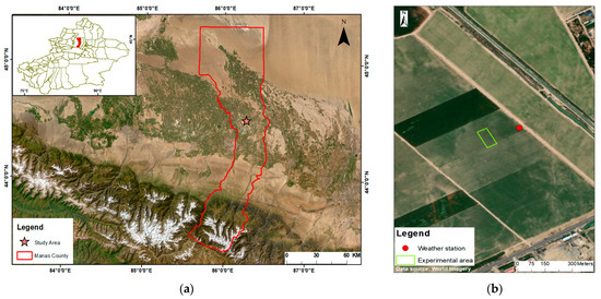
Figure 1. Location of the study area and field experimental area. (a) The geographical location of Manas County, Xinjiang, China, with the study area outlined in red and the star marking the location of the experimental site. (b) The experimental area is approximately 3 ha and is outlined in green, and the red dots indicate the locations of weather stations.

2.2. Experimental Design

A randomized complete block design was employed with four irrigation levels, 0% (T1), 30% (T2), 60% (T3), and 90% (T4) of the local irrigation amount (Table 1), each replicated three times. Cotton was sown following the “one-film six-row three-belt” pattern, with a film width of 2.05 m, row spacing of 10 cm, and inter-film spacing of 66 cm. One drip line was installed on each side of the planting belt to ensure precise irrigation. Field management followed local agronomic practices. The planting density was 270,000 plants per hectare. Irrigation treatments began at 59 days after planting (DAP) in 2024. After treatment initiation, the 0% treatment (T1) received no further irrigation. This treatment served as the rain-fed reference (no irrigation) and marked the lower end of the irrigation gradient.

Table 1. The irrigation schedule of different treatments in the study field.

Day After Planting (DAP)	Irrigation Treatment (m3/ha)
	30%	60%	90%
6	300	300	300
59	81	162	243
71	82.5	165	247.5
79	126	252	378
90	123	246	369
97	127.5	255	382.5
106	124.5	249	373.5
114	93	186	279
120	90	180	270
127	91.5	183	274.5

2.3. Data Acquisition

2.3.1. UAS Image Data Acquisition

High-resolution multispectral images were acquired at three key crop growth stages using a Pegasus D2000S UAS (Feima, Beijing China) equipped with a D-MSPC2000 multispectral sensor (Feima, Beijing, China) (Figure 2). The sensor captures reflectance across six spectral bands: blue (450 nm), green (555 nm), red (660 nm), red-edge 1 (720 nm), red-edge 2 (750 nm), and NIR (840 nm). Flight missions were planned and executed in Pix4D (v4.5.6, Prilly, Switzerland). Image acquisition was carried out within ~1 h around local solar noon (13:00–14:00). Flights were conducted at 60 m altitude and 7.2 m/s, using 75% front and side overlap, yielding an approximate ground sampling distance of 10 cm. Radiometric calibration was performed prior to each flight using a standard reflectance panel to ensure image consistency. During the 2024 growing season, multispectral imagery and ground-based LAI data were collected simultaneously (Table 2). Field experiments and drone observations were conducted on days 63, 80, and 101 DAP, with 36 sampling points set up each time, resulting in a total of 108 sampling points.

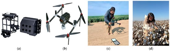
Figure 2. UAS-based multispectral imaging system and field measurements. (a) D-MSPC2000 multispectral sensor; (b) Pegasus D2000S UAS system; (c) reflectance calibration with reference panels; (d) yield measurement.

Table 2. UAS image acquisition during different stages of cotton growth in 2024.

Year	Day After Planting (DAP)	UAS Sensor	Cotton Growth Stage
2024	63	Multispectral	Squaring (early-mid-season)
	80	Multispectral	Flowering (mid-season)
	101	Multispectral	Boll-setting (mid-late-season)

2.3.2. Field Data Collection

The ground measurement of the LAI was conducted 63, 80, and 101 days after planting. On each sampling date, three uniform cotton plants were randomly selected within each plot, covering an area of approximately 3 m². Individual leaf areas of each plant were measured using a Leaf-1000 sensor (Shangsheng Instrument Co., Ltd., Hangzhou, China) and summed to obtain total leaf area per plant. The measured leaf area was then divided by the corresponding ground projection area to calculate the plot-level LAI, which served as ground reference data.

Plant density was determined by counting all plants within each plot. In each plot, 10 plants were randomly selected for yield measurement. The bolls per plant were counted and weighed. Yield of each plot (kg/ha) was calculated based on boll weight and plant density

2.4. Data Processing

Multispectral images were stitched using Pix4D to generate orthorectified reflectance maps through mosaicking [38,39], geometric correction, and radiometric calibration. In the processed images, RED, GREEN, BLUE, NIR, and RedEdge denote the surface reflectance in the red, green, blue, near-infrared, and red-edge bands, respectively. For each sampling site, a 300 × 300-pixel region (10 cm × 10 cm resolution) was extracted to calculate mean reflectance, matched to the corresponding measured LAI. Eleven vegetation indices were derived from the reflectance data (Table 3) [40,41].

Pearson correlation analysis was performed to assess relationships between vegetation indices and measured LAI [42,43]. The index showing the strongest correlation with LAI was then chosen as the predictor. Using this predictor, three inversion models—linear regression (LR), random forest (RF), and support vector machine (SVR)—were developed [44]. The dataset was divided into 70% for training and 30% for validation. Model performance was assessed using the coefficient of determination (R²) and the root mean square error (RMSE). Finally, the model with the highest accuracy was selected to generate UAS-LAI, which was then used as input data for the calibration and assimilation of the DSSAT model.

Table 3. Vegetation indices and their calculation formulas for cotton derived from multispectral imagery.

VIs	Value Range	Description	Calculation Formula	Refs
NDVI	[−1, 1]	Higher values indicating denser vegetation	$\mathrm{N}\mathrm{D}\mathrm{V}\mathrm{I}={\displaystyle \frac{\mathrm{N}\mathrm{I}\mathrm{R}-\mathrm{R}\mathrm{E}\mathrm{D}}{\mathrm{N}\mathrm{I}\mathrm{R}+\mathrm{R}\mathrm{E}\mathrm{D}}}$	[45]
EVI	[−1, 1]	Less saturation in dense canopy	$\mathrm{E}\mathrm{V}\mathrm{I}=2.5\times {\displaystyle \frac{\mathrm{N}\mathrm{I}\mathrm{R}-\mathrm{R}\mathrm{E}\mathrm{D}}{\mathrm{N}\mathrm{I}\mathrm{R}+6\times \mathrm{R}\mathrm{E}\mathrm{D}-7.5\times \mathrm{B}\mathrm{L}\mathrm{U}\mathrm{E}+1}}$	[46]
NDRE	[−1, 1]	Higher values indicate higher chlorophyll	$\mathrm{N}\mathrm{D}\mathrm{R}\mathrm{E}={\displaystyle \frac{\mathrm{N}\mathrm{I}\mathrm{R}-\mathrm{R}\mathrm{e}\mathrm{d}\mathrm{E}\mathrm{d}\mathrm{g}\mathrm{e}}{\mathrm{N}\mathrm{I}\mathrm{R}+\mathrm{R}\mathrm{e}\mathrm{d}\mathrm{E}\mathrm{d}\mathrm{g}\mathrm{e}}}$	[47]
GNDVI	[−1, 1]	Estimate the moisture and nitrogen conditions within the tree canopy	$\mathrm{G}\mathrm{N}\mathrm{D}\mathrm{V}\mathrm{I}={\displaystyle \frac{\mathrm{N}\mathrm{I}\mathrm{R}-\mathrm{G}\mathrm{R}\mathrm{E}\mathrm{E}\mathrm{N}}{\mathrm{N}\mathrm{I}\mathrm{R}+\mathrm{G}\mathrm{R}\mathrm{E}\mathrm{E}\mathrm{N}}}$	[48]
TVI	[>0]	Vegetation vigor index	$\mathrm{T}\mathrm{V}\mathrm{I}=\sqrt{120\times (\mathrm{N}\mathrm{I}\mathrm{R}-\mathrm{R}\mathrm{E}\mathrm{D})-200\times (\mathrm{G}\mathrm{R}\mathrm{E}\mathrm{E}\mathrm{N}-\mathrm{R}\mathrm{E}\mathrm{D})}$	[49]
MSAVI	[−1, 1]	Higher values mean denser vegetation and less soil effect	$\mathrm{M}\mathrm{S}\mathrm{A}\mathrm{V}\mathrm{I}=(2\mathrm{N}\mathrm{I}\mathrm{R}+1-\mathrm{s}\mathrm{q}\mathrm{r}\mathrm{t}((2\mathrm{N}\mathrm{I}\mathrm{R}+1{)}^2-8\times (\mathrm{N}\mathrm{I}\mathrm{R}-\mathrm{R}\mathrm{e}\mathrm{d}\left)\right))/2$	[50]
OSAVI	[−1, 1]	Reduces soil background effects and is suitable for early canopy growth	$\mathrm{O}\mathrm{S}\mathrm{A}\mathrm{V}\mathrm{I}={\displaystyle \frac{\mathrm{N}\mathrm{I}\mathrm{R}-\mathrm{R}\mathrm{E}\mathrm{D}}{\mathrm{N}\mathrm{I}\mathrm{R}+\mathrm{R}\mathrm{E}\mathrm{D}+0.16}}$	[51]
GCI	[≥0]	Related to leaf chlorophyll/nitrogen	$\mathrm{G}\mathrm{C}\mathrm{I}={\displaystyle \frac{\mathrm{N}\mathrm{I}\mathrm{R}}{\mathrm{G}\mathrm{R}\mathrm{E}\mathrm{E}\mathrm{N}}}$	[52]
CCI	[≥0]	Canopy chlorophyll index; red-edge is more sensitive	$\mathrm{C}\mathrm{C}\mathrm{I}={\displaystyle \frac{\mathrm{N}\mathrm{I}\mathrm{R}-\mathrm{R}\mathrm{e}\mathrm{d}\mathrm{E}\mathrm{d}\mathrm{g}\mathrm{e}}{\mathrm{N}\mathrm{I}\mathrm{R}-\mathrm{R}\mathrm{E}\mathrm{D}}}$	[53]
DVI	Depends on reflectance scale	Reflects the changes in vegetation coverage	$\mathrm{D}\mathrm{V}\mathrm{I}=\mathrm{N}\mathrm{I}\mathrm{R}-\mathrm{R}\mathrm{E}\mathrm{D}$	[54]
MTVI	No fixed range	Reduced saturation under dense vegetation	$\mathrm{M}\mathrm{T}\mathrm{V}\mathrm{I}=1.2\times [1.2\times (\mathrm{N}\mathrm{I}\mathrm{R}-\mathrm{G}\mathrm{R}\mathrm{E}\mathrm{E}\mathrm{N})-2.5\times (\mathrm{R}\mathrm{E}\mathrm{D}-\mathrm{G}\mathrm{R}\mathrm{E}\mathrm{E}\mathrm{N}\left)\right]$	[55]

Table 3. Vegetation indices and their calculation formulas for cotton derived from multispectral imagery.

VIs	Value Range	Description	Calculation Formula	Refs
NDVI	[−1, 1]	Higher values indicating denser vegetation	$\mathrm{N}\mathrm{D}\mathrm{V}\mathrm{I}={\displaystyle \frac{\mathrm{N}\mathrm{I}\mathrm{R}-\mathrm{R}\mathrm{E}\mathrm{D}}{\mathrm{N}\mathrm{I}\mathrm{R}+\mathrm{R}\mathrm{E}\mathrm{D}}}$	[45]
EVI	[−1, 1]	Less saturation in dense canopy	$\mathrm{E}\mathrm{V}\mathrm{I}=2.5\times {\displaystyle \frac{\mathrm{N}\mathrm{I}\mathrm{R}-\mathrm{R}\mathrm{E}\mathrm{D}}{\mathrm{N}\mathrm{I}\mathrm{R}+6\times \mathrm{R}\mathrm{E}\mathrm{D}-7.5\times \mathrm{B}\mathrm{L}\mathrm{U}\mathrm{E}+1}}$	[46]
NDRE	[−1, 1]	Higher values indicate higher chlorophyll	$\mathrm{N}\mathrm{D}\mathrm{R}\mathrm{E}={\displaystyle \frac{\mathrm{N}\mathrm{I}\mathrm{R}-\mathrm{R}\mathrm{e}\mathrm{d}\mathrm{E}\mathrm{d}\mathrm{g}\mathrm{e}}{\mathrm{N}\mathrm{I}\mathrm{R}+\mathrm{R}\mathrm{e}\mathrm{d}\mathrm{E}\mathrm{d}\mathrm{g}\mathrm{e}}}$	[47]
GNDVI	[−1, 1]	Estimate the moisture and nitrogen conditions within the tree canopy	$\mathrm{G}\mathrm{N}\mathrm{D}\mathrm{V}\mathrm{I}={\displaystyle \frac{\mathrm{N}\mathrm{I}\mathrm{R}-\mathrm{G}\mathrm{R}\mathrm{E}\mathrm{E}\mathrm{N}}{\mathrm{N}\mathrm{I}\mathrm{R}+\mathrm{G}\mathrm{R}\mathrm{E}\mathrm{E}\mathrm{N}}}$	[48]
TVI	[>0]	Vegetation vigor index	$\mathrm{T}\mathrm{V}\mathrm{I}=\sqrt{120\times (\mathrm{N}\mathrm{I}\mathrm{R}-\mathrm{R}\mathrm{E}\mathrm{D})-200\times (\mathrm{G}\mathrm{R}\mathrm{E}\mathrm{E}\mathrm{N}-\mathrm{R}\mathrm{E}\mathrm{D})}$	[49]
MSAVI	[−1, 1]	Higher values mean denser vegetation and less soil effect	$\mathrm{M}\mathrm{S}\mathrm{A}\mathrm{V}\mathrm{I}=(2\mathrm{N}\mathrm{I}\mathrm{R}+1-\mathrm{s}\mathrm{q}\mathrm{r}\mathrm{t}((2\mathrm{N}\mathrm{I}\mathrm{R}+1{)}^2-8\times (\mathrm{N}\mathrm{I}\mathrm{R}-\mathrm{R}\mathrm{e}\mathrm{d}\left)\right))/2$	[50]
OSAVI	[−1, 1]	Reduces soil background effects and is suitable for early canopy growth	$\mathrm{O}\mathrm{S}\mathrm{A}\mathrm{V}\mathrm{I}={\displaystyle \frac{\mathrm{N}\mathrm{I}\mathrm{R}-\mathrm{R}\mathrm{E}\mathrm{D}}{\mathrm{N}\mathrm{I}\mathrm{R}+\mathrm{R}\mathrm{E}\mathrm{D}+0.16}}$	[51]
GCI	[≥0]	Related to leaf chlorophyll/nitrogen	$\mathrm{G}\mathrm{C}\mathrm{I}={\displaystyle \frac{\mathrm{N}\mathrm{I}\mathrm{R}}{\mathrm{G}\mathrm{R}\mathrm{E}\mathrm{E}\mathrm{N}}}$	[52]
CCI	[≥0]	Canopy chlorophyll index; red-edge is more sensitive	$\mathrm{C}\mathrm{C}\mathrm{I}={\displaystyle \frac{\mathrm{N}\mathrm{I}\mathrm{R}-\mathrm{R}\mathrm{e}\mathrm{d}\mathrm{E}\mathrm{d}\mathrm{g}\mathrm{e}}{\mathrm{N}\mathrm{I}\mathrm{R}-\mathrm{R}\mathrm{E}\mathrm{D}}}$	[53]
DVI	Depends on reflectance scale	Reflects the changes in vegetation coverage	$\mathrm{D}\mathrm{V}\mathrm{I}=\mathrm{N}\mathrm{I}\mathrm{R}-\mathrm{R}\mathrm{E}\mathrm{D}$	[54]
MTVI	No fixed range	Reduced saturation under dense vegetation	$\mathrm{M}\mathrm{T}\mathrm{V}\mathrm{I}=1.2\times [1.2\times (\mathrm{N}\mathrm{I}\mathrm{R}-\mathrm{G}\mathrm{R}\mathrm{E}\mathrm{E}\mathrm{N})-2.5\times (\mathrm{R}\mathrm{E}\mathrm{D}-\mathrm{G}\mathrm{R}\mathrm{E}\mathrm{E}\mathrm{N}\left)\right]$	[55]

2.5. Basic Data for DSSAT Modeling

The DSSAT is a process-based cropping system modeling framework composed of interacting modules for crop growth, soil, weather, and management, which simulate daily soil–plant–atmosphere dynamics [56]. In this study, the DSSAT-CSM cotton module (CSM-CROPGRO-Cotton) was used to simulate crop development, canopy growth, and yield formation under different irrigation conditions. These inputs were compiled by integrating field measurements with publicly available data to generate model input files for parameter calibration and simulation (Table 4). The meteorological data are organized into daily records. Among them, solar radiation is calculated using the Ångström–Prescott (sunshine duration) method based on the sunshine duration:

$$R_s=(a_s+b_s{\displaystyle \frac{n}{N}})R_a$$

(1)

Table 4. DSSAT simulations utilized meteorological, soil, and crop management data.

Data Type	Specific Variables	Source	DSSAT Files/Parameters
Weather	Max/min temperature, precipitation, sunshine hours, solar radiation, etc.	Weather station	Weather file (*. WTH), solar radiation estimated from sunshine hours.
Soil	Texture, water content, organic carbon, pH, layer depth, soil bulk density, saturation moisture content, etc.	Field sampling and lab analysis (0–40 cm)	Soil file (*. SOL) for water and nutrient simulation.
Management	Sowing date, planting distance, irrigation date, irrigation method, crop variety parameters, etc.	Field records	Management file (*. X) for scenario definition.

“*” denotes the DSSAT file-type wildcard (e.g., *. WTH weather file, *. SOL soil file, *. X management file).

Here, n is the measured sunshine duration, $N$ is the maximum possible sunshine duration, and $R_a$ is the extraterrestrial radiation ($\mathrm{M}\mathrm{J}{\mathrm{m}}^{-2}{\mathrm{d}}^{-1}$), calculated from latitude and day of year. In the absence of local calibration, $a_s$ and $b_s$ were set to 0.25 and 0.50, respectively [57].

Soil samples were collected in the experimental field and analyzed for soil properties in the laboratory, including texture, moisture content, organic carbon, pH value, soil bulk density, saturated moisture content, etc. Detailed field management data was recorded, including planting density, row spacing, irrigation plan, harvest date, etc. The genetic parameters of the cultivated cotton varieties were obtained from publicly available sources and incorporated into the model. These parameters were used for calibration to ensure that the simulated growth and yield accurately reflected field conditions.

2.6. PSO-Based Parameter Calibration and LAI Assimilation

Based on the input datasets, the DSSAT-CROPGRO-Cotton model was calibrated using field-measured and UAS-derived LAI data (Figure 3). The Particle Swarm Optimization (PSO) algorithm is a population-based optimizer that updates candidate solutions (“particles”) using both personal-best and global-best information [58]. It was used to automatically calibrate key genetic parameters to improve yield simulation accuracy under different irrigation conditions. In each iteration, a set of parameters generated by PSO was input into the DSSAT to simulate the LAI. The mean squared error (MSE) between the simulated and observed LAI was used as the objective function. PSO was implemented with a swarm size of 50; the inertia weight (w) was linearly decreased from 0.9 to 0.4; and the acceleration coefficients were set to c1 = 2.0 and c2 = 2.0, with a maximum of 500 iterations [59]. The optimization continued until MSE reached its minimum, yielding the optimal parameter set capable of accurately reproducing LAI dynamics:

$$\mathrm{M}\mathrm{S}\mathrm{E}={\displaystyle \frac{1}{n}}{\sum }_{i=1}^n{\left(\mathrm{L}\mathrm{A}{\mathrm{I}}_{\mathrm{sim},\mathrm{i}}-\mathrm{L}\mathrm{A}{\mathrm{I}}_{\mathrm{obs},\mathrm{i}}\right)}^2,$$

(2)

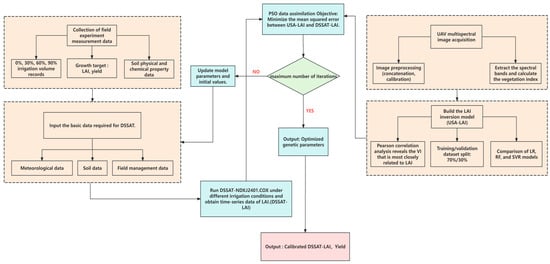
Figure 3. Research technology flowchart.

In Equation (2), $\mathrm{L}\mathrm{A}{\mathrm{I}}_{\mathrm{sim},\mathrm{i}}$ and $\mathrm{L}\mathrm{A}{\mathrm{I}}_{\mathrm{obs},\mathrm{i}}$ represent simulated and observed LAI on the i DAP. The evaluation was performed at 63, 80, and 101 DAP, corresponding to the blooming, flowering, and boll-filling stages.

The objective function aims to minimize UAS-LAI simulation errors at critical growth stages, thereby ensuring greater physiological consistency in the optimized model. On this basis, the UAS-LAI data were further assimilated into the DSSAT model as observational constraints to improve the accuracy of simulated LAI temporal dynamics. Data assimilation was implemented only under the 30%, 60%, and 90% irrigation treatments, with observations introduced at three key phenological stages to adjust the simulated LAI trajectory. The optimal parameter set obtained through PSO calibration (EM-FL, FL-SH, LFMAX, SLAVR, SIZLF, XFRT) was then used to construct the calibrated model (Table 5), in which the assimilated LAI time series served as an additional input driving crop growth and yield formation throughout the growing season [60].

Table 5. Initial value and tuning range of model parameters to be optimized.

Parameters	Description	Initial Value	Range
EM-FL	Time from emergence to flowering.	45	29~45
FL-SH	Time from flowering to shoot harvest.	11	10~13
LFMAX	Maximum leaf area.	1.2	0.7~1.2
SLAVR	Specific leaf area (leaf area per unit dry mass).	180	90~250
SIZLF	Leaf size.	230	170~230
XFRT	Fruit set or fruiting period.	0.69	0.5~0.9

To ensure the stability and reliability of the simulations, simulated seed cotton yield was compared with field observations. The model performance was evaluated using RMSE and R², as defined by the following equations, and statistical significance was assessed for the linear regression model using p-values at the 95% confidence level (α = 0.05):

$$\mathrm{R}\mathrm{M}\mathrm{S}\mathrm{E}=\sqrt{{\displaystyle \frac{1}{\mathrm{n}}}{\sum }_{\mathrm{i}=1}^{\mathrm{n}}{\left(\mathrm{L}\mathrm{A}{\mathrm{I}}_{\mathrm{s}\mathrm{i}\mathrm{m},\mathrm{i}}-\mathrm{L}\mathrm{A}{\mathrm{I}}_{\mathrm{o}\mathrm{b}\mathrm{s},\mathrm{i}}\right)}^2},$$

(3)

$${\mathrm{R}}^2={\left({\displaystyle \frac{\sum _{\mathrm{i}=1}^{\mathrm{n}}\left(\mathrm{L}\mathrm{A}{\mathrm{I}}_{\mathrm{s}\mathrm{i}\mathrm{m},\mathrm{i}}-{\overline{\mathrm{L}\mathrm{A}\mathrm{I}}}_{\mathrm{s}\mathrm{i}\mathrm{m}}\right)\left(\mathrm{L}\mathrm{A}{\mathrm{I}}_{\mathrm{o}\mathrm{b}\mathrm{s},\mathrm{i}}-{\overline{\mathrm{L}\mathrm{A}\mathrm{I}}}_{\mathrm{o}\mathrm{b}\mathrm{s}}\right)}{\sqrt{\sum _{\mathrm{i}=1}^{\mathrm{n}}{\left(\mathrm{L}\mathrm{A}{\mathrm{I}}_{\mathrm{s}\mathrm{i}\mathrm{m},\mathrm{i}}-{\overline{\mathrm{L}\mathrm{A}\mathrm{I}}}_{\mathrm{s}\mathrm{i}\mathrm{m}}\right)}^2}\sqrt{\sum _{\mathrm{i}=1}^{\mathrm{n}}{\left(\mathrm{L}\mathrm{A}{\mathrm{I}}_{\mathrm{o}\mathrm{b}\mathrm{s},\mathrm{i}}-{\overline{\mathrm{L}\mathrm{A}\mathrm{I}}}_{\mathrm{o}\mathrm{b}\mathrm{s}}\right)}^2}}}\right) }^2,$$

(4)

where $\mathrm{L}\mathrm{A}{\mathrm{I}}_{\mathrm{sim},\mathrm{i} }\mathrm{a}\mathrm{n}\mathrm{d} \mathrm{L}\mathrm{A}{\mathrm{I}}_{\mathrm{obs},\mathrm{i}}$ represent the simulated and observed values on the i day, and ${\overline{\mathrm{L}\mathrm{A}\mathrm{I}}}_{\mathrm{s}\mathrm{i}\mathrm{m}}$ and ${\overline{\mathrm{L}\mathrm{A}\mathrm{I}}}_{\mathrm{o}\mathrm{b}\mathrm{s}}$ are their corresponding mean values. Lower RMSE and higher R² indicate closer agreement between simulated and observed values.

2.7. Data Analysis

Pearson’s correlation coefficient (r) and a two-tailed p-value were computed to quantify associations between the LAI and the vegetation indices. These statistics were computed in Python (Anaconda; v3.12.4) using NumPy (v1.26.4), Pandas (v2.2.3), and SciPy (v1.14.1). The results were organized into a correlation matrix and visualized as a heatmap with Matplotlib (v3.7.1) and Seaborn (v0.13.2). Three regression models (LR, SVR, and RF) were applied to model VIs–LAI relationships. LR provided a linear baseline. SVR accounted for potential nonlinear responses, with key hyperparameters including $C$,$ϵ$, and kernel configuration (e.g., RBF kernel with $\gamma$) [61]. RF was configured using the number of trees $(n\_estimators)$ and tree-structure constraints (e.g., maximum depth). All models were implemented in Python with scikit-learn (v1.5.2). Given the limited sample size, model generalization was assessed using 5-fold cross-validation (k = 5), and performance was summarized by the mean metrics across folds [62]. Model accuracy was evaluated using R², RMSE, and MAE, which were used to compare LR, SVR, and RF in terms of predictive stability.

The overall workflow of the data processing, analysis, and modeling procedure is summarized in Figure 3.

3. Results

3.1. The Relationship Between VIs and Cotton LAI over the Growing Season

The relationship between vegetation indices (VIs) and cotton LAI was examined at different growth stages (Figure 4). At the square stage (63 DAP), there was no significant correlation between the NDRE, CCI, and LAI. The other VIs were significantly correlated with the LAI (p < 0.05), with the NDVI showing the highest correlation (r = 0.65), followed by the OSAVI and MTVI (r = 0.61). At the flowering stage (80 DAP), the MTVI showed the highest correlation with the LAI. In the boll-opening stage (101 DAP), the canopy was nearly closed, and the NDRE, GNDVI, GCI, and CCI remained uncorrelated with the LAI, while the EVI, TVI, and MTVI exhibited the highest correlations (r > 0.77). This result indicated that VIs have great potential for estimating cotton LAIs in different growth stages. However, due to differences in surface coverage and band characteristics, the correlation between VIs and the LAI varies in different growth stages. A scatter plot of VIs and the LAI is shown in Figure 5. In this study, the NDVI showed higher accuracy in estimating the LAI during the early growth stage, while the MTVI and EVI showed higher and more stable accuracy in estimating the LAI during the late growth stages. The main reason for this difference is that in the later stage of the dense cotton plant community, when the LAI is greater than 3, NDVI often reaches a saturation state, which leads to a decrease in its sensitivity and makes it difficult to capture the further increase in the LAI in the subsequent stages. This phenomenon is widely regarded as a typical spectral feature in the middle and late stages of plant canopy growth.

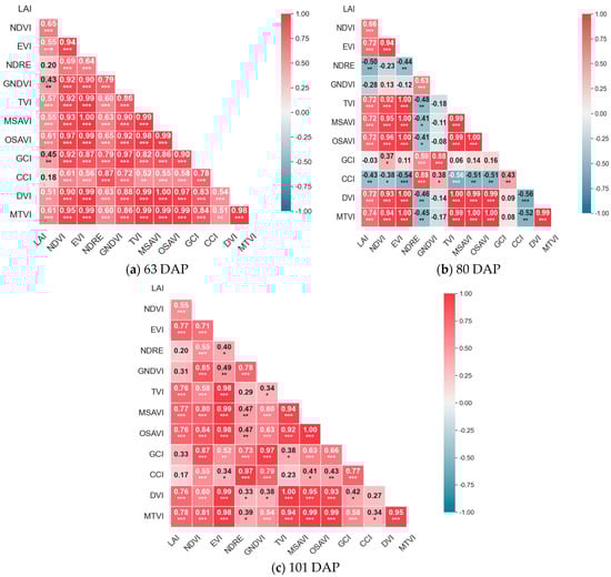
Figure 4. Pearson correlation between vegetation indices and LAI at different stages: (a) squaring (63 DAP, early-mid-season); (b) flowering (80 DAP, mid-season); (c) boll-setting (101 DAP, mid-late-season). Red/blue indicates positive/negative correlation; color intensity reflects strength. *, **, and *** indicate p < 0.05, 0.01, and 0.001; no asterisk means non-significant (p ≥ 0.05).

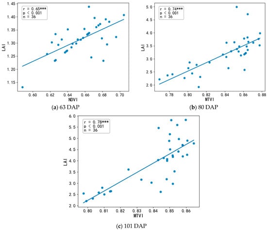
Figure 5. Scatter plots showing the correlations between vegetation indices and measured LAI at three phenological stages: (a) NDVI–LAI (63 DAP), (b) MTVI–LAI (80 DAP), and (c) MTVI–LAI (101 DAP). The legend shows the Pearson correlation coefficient, p-value, and sample size; lines indicate linear fits. *** Indicates p < 0.001.

3.2. The Performance of Different Models in LAI Estimation

The performance of different regression algorithms for UAS-LAI retrieval was evaluated by comparing the LR, SVR, and RF models across three critical growth stages of cotton (Table 6). The results indicate that the LR model outperformed the other algorithms across all growth stages, with the values of R² ranging from 0.56 to 0.76 (Figure 6). Specifically, at the 63 DAP stage, the LR model based on the NDVI achieved the highest accuracy (R² = 0.56); at the 80 DAP stage, the LR model based on the MTVI showed the best fitting performance (R² = 0.64); and at 101 DAP, the LR model maintained its superior performance (R² = 0.76). In contrast, the performance of the SVR and RF models exhibited greater variability, with their overall predictive accuracy being lower than that of the LR model. Based on these results, the LR model was selected as the optimal algorithm for UAS-LAI retrieval.

Table 6. Performance of LR, SVR, and RF models for LAI estimation at different DAP using the selected vegetation indices. Evaluation results are presented as mean ± standard deviation from 5-fold cross-validation (k = 5), root mean square error (RMSE), and mean absolute error (MAE).

DAP	Vegetation Index	LR			SRV			RF
		R2	RESE	MAE	R2	RESE	MAE	R2	RESE	MAE
63	NDVI	0.30 ± 0.21	0.05 ± 0.01	0.04 ± 0.01	−0.20 ± 0.46	0.06 ± 0.02	0.05 ± 0.02	−0.32 ± 0.57	0.07 ± 0.03	0.05 ± 0.02
80	MTVI	0.56 ± 0.36	0.42 ± 0.25	0.34 ± 0.19	0.55 ± 0.36	0.42 ± 0.25	0.34 ± 0.19	0.21 ± 0.50	0.52 ± 0.22	0.41 ± 0.18
101	MTVI	0.68 ± 0.23	0.52 ± 0.14	0.43 ± 0.14	0.59 ± 0.17	0.62 ± 0.16	0.48 ± 0.16	0.67 ± 0.10	0.57 ± 0.14	0.45 ± 0.14

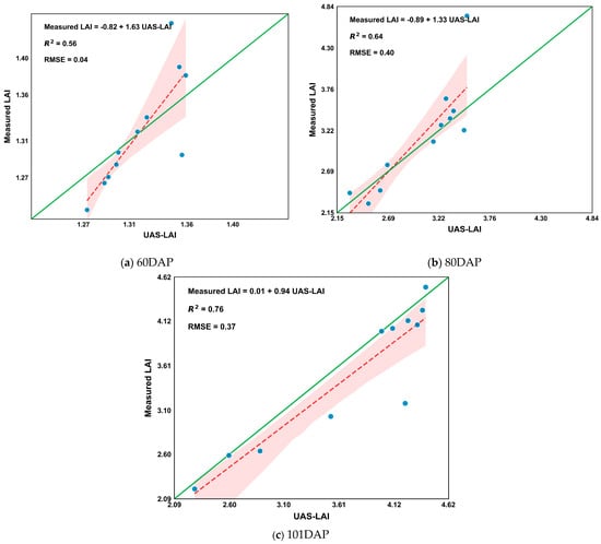
Figure 6. The relationship between measured LAI and UAS-LAI at three growth stages (63, 80, and 101 DAP): (a) squaring; (b) flowering; (c) boll-setting. This shows the scatter plot obtained based on the 7:3 training set and test set division. The green line represents the 1:1 line, and the red dashed line represents the regression line. The shaded area indicates the 95% confidence interval of the regression model.

3.3. Cotton Growth Simulation Based on UAS Assimilation DSSAT Model

The optimization of key genetic parameters in the DSSAT model using the Particle Swarm Optimization (PSO) algorithm was followed through the assimilation of UAS-LAI data under different irrigation treatments as state variables to dynamically correct the simulation process. Figure 7 presents DSSAT simulations for the irrigated treatments (30%, 60%, and 90%). Before assimilation, the model consistently underestimated LAI across all irrigation conditions, particularly during the rapid growth phase between 60 and 100 days after sowing. During this period, both the growth rate and peak magnitude of the LAI were significantly lower than the observed values, indicating low simulation accuracy in the absence of assimilation data.

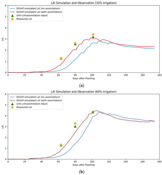
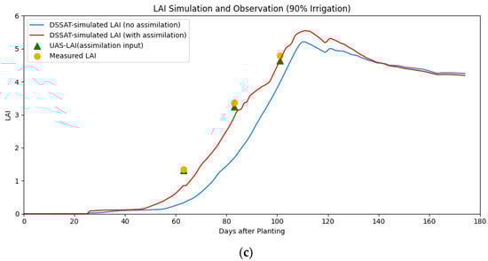
Figure 7. Comparison of DSSAT-simulated LAI with and without assimilation and remote sensing-derived LAI under 30%, 60%, and 90% irrigation treatments. Blue lines: DSSAT-simulated LAI without assimilation; red lines: with assimilation; green triangles: remote sensing-derived LAI used for assimilation; yellow points: measured LAI. Subplots (a), (b), and (c) show results for 30%, 60%, and 90% irrigation, respectively.

After assimilation, the simulated LAI values became much closer to the measured LAI. For example, under 30% irrigation, the simulated LAI on day 101 (green triangle) matched well with the measured LAI, validating the effectiveness of the assimilation process. Under 60% irrigation, the model successfully captured the cotton growth acceleration phase between days 80 and 101, with simulated values aligning well with both UAS-LAI and the measured data. Under 90% irrigation, the assimilated model (red line) successfully captured the LAI peak on day 101, and the predicted growth rate was consistent with the observed data (orange circles).

Overall, the assimilation of the UAS-LAI data significantly enhanced the DSSAT model’s ability to simulate LAI dynamics under different irrigation conditions, particularly during critical growth stages. The data assimilation effectively corrected model biases, providing a more stable and reliable input for cotton simulation and subsequent yield prediction.

3.4. Yield Prediction Using Assimilated DSSAT Model

Figure 8 shows the cotton yield difference under different irrigation treatments of measurement (red bars), simulation before calibration (blue bars), and simulation after calibration (green bars). Across the three irrigation treatments, the pre-calibration DSSAT-simulated yields showed no significant difference between the 90% and 60% treatments, whereas both were significantly higher than that of the 30% treatment (p < 0.05). In contrast, the measured yield of the 90% treatment was significantly greater than that of the 60% treatment (p < 0.05), while no significant difference was detected between the 30% and 60% treatments. For the post-calibration DSSAT-simulated yields, significant differences existed among all three irrigation treatments (p < 0.05).

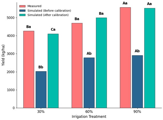
Figure 8. Comparison of measured yield and DSSAT model simulations under different irrigation treatments (30%, 60%, and 90%). Red bars represent observed yield, blue bars represent simulated yield before calibration, and green bars represent simulated yield after calibration. Capital letters indicate the significant differences resulting from different irrigation treatment methods (analyzed using one-way analysis of variance and combined with the Tukey-HSD method for testing, with p < 0.05). The lowercase letters indicate significant differences among the measured yiled, simulated yield (before calibration), and simulated yield (after calibration) within each irrigation treatment.

Under three irrigation treatment conditions, the errors in cotton yield between the simulated (before calibration) results and the measured values are 52.4% (30% irrigation), 40.8% (60% irrigation), and 47.6% (90% irrigation). After calibration, there was no significant difference between the simulated results of the model and the field measurement, with an error of 3.6–6.3%. The simulated accuracy has been improved by 93.1%, 84.6%, and 98.4%. This indicates that errors in LAI simulation weakened the model’s sensitivity to water stress. The assimilation of the LAI effectively corrected the systematic biases of the DSSAT model under water stress conditions, significantly improving the accuracy and stability of yield predictions. This process enhanced the reliability of key physiological variables, strengthening the model’s applicability under varying water conditions.

4. Discussion

The LAI, as a key indicator of plant photosynthetic capacity, directly influences the assessment of crop growth stages and yield simulations [63,64]. Studies have shown that VI–LAI relationships can shift across growth stages [65]. Such shifts are expected as canopy architecture and leaf optical traits evolve through the season, altering spectral sensitivity and increasing the likelihood of saturation at higher LAI [66]. This saturation effect, and its resulting limitation on LAI retrieval under closed-canopy conditions, has been widely documented and is comprehensively summarized in Yan et al.’s review of vegetation indices [67]. During early growth stages with sparse canopies, structure-sensitive indices such as the NDVI and MTVI effectively capture leaf area expansion, whereas these indices tend to saturate as the canopy closes, reducing inversion accuracy. In later growth stages, red-edge indices (e.g., NDRE and CCI) are more sensitive to variations in leaf nitrogen and chlorophyll content, which can weaken their linkage to the LAI when leaves senesce and chlorophyll declines; under such conditions, red-edge signals increasingly reflect pigment changes rather than canopy leaf area. Sun et al. and Li et al. highlighted that reducing chlorophyll-driven variability is critical for robust LAI estimation, particularly when pigment dynamics are not synchronized with structural LAI changes during late-season senescence [68,69]. Their stability declines under closed-canopy conditions and environmental interference [70]. In this study, the MTVI tended to outperform the red-edge indices (NDRE and CCI) because it is more responsive to canopy structure and fractional cover, whereas the NDRE and CCI are more strongly influenced by chlorophyll-driven red-edge signals. During the late growth stages, cotton leaves gradually senesced, and chlorophyll content declined; consequently, NDRE and CCI increasingly captured pigment dynamics rather than changes in canopy leaf area, weakening their relationship with the LAI. Moreover, under relatively dense canopies, red-edge indices can exhibit reduced sensitivity (partial saturation) to further LAI variations. These findings indicate that the effectiveness of LAI inversion depends not only on the intrinsic performance of vegetation indices but also on their alignment with canopy photosynthetic and growth dynamics at different developmental stages. Beyond the choice of vegetation indices, the regression model used to translate spectral features into LAI can further influence the stability of inversion across growth stages. In this study, more complex models (SVR and RF) did not outperform linear regression (LR) for LAI retrieval. This is likely because the dataset contained a limited number of samples and only a few observation dates, and the VI features already captured most of the LAI-related variation; therefore, introducing additional nonlinear flexibility provided little extra gain. In addition, SVR and RF are more dependent on hyperparameter settings and can be more sensitive to sampling variability and measurement noise, which may weaken generalization when the dataset is small. Accordingly, LR was selected as a stable and interpretable model for LAI estimation in this study.

Assimilating UAS-LAI as a single-variable input, combined with PSO-optimized key genetic parameters, can substantially enhance the simulation accuracy of the DSSAT model [71,72,73]. As a critical state variable, LAI precision directly affects the model’s ability to simulate growth stages and predict yield [74]. Unassimilated models rely on fixed genetic parameters and lack responsiveness to real-time environmental changes, resulting in pronounced biases in canopy development and water stress simulation [75]. Specifically, during early canopy stages, unassimilated models underestimate leaf area expansion and potential photosynthetic rates, leading to slower LAI growth and lower peak values [76]. Between 60 and 100 days, a key developmental window, water stress effects on canopy structure are inadequately captured, increasing discrepancies between simulated and observed LAI values. In addition, multivariable assimilation may introduce redundant information when observational data are insufficient or noisy, potentially destabilizing model performance. Although the PSO algorithm provides robust global search capabilities, its effectiveness is constrained by the initial parameter range settings [77]. Moreover, under extreme water stress or closed-canopy conditions, the model’s ability to simulate nonlinear responses is limited, which may result in flattened or failed LAI simulations and compromise yield predictions [78]. In this study, although there are still uncertainties due to data resolution, observation frequency, and extreme environmental conditions, the use of PSO and LAI assimilation significantly improved model performance [79,80]. The LAI estimation based on vegetation indices and the DSSAT calibration framework performed well in the experimental area. However, the evaluation was limited to one site and one growing season, and no independent datasets from other locations or years were available for external validation. Further research will be conducted in different regions, under different cultivation management conditions and varieties, to verify the method and enhance its robustness and applicability.

In future research, multi-source remote sensing data, including hyperspectral and thermal infrared images, should be integrated to further improve the accuracy of LAI inversion. The fusion of multiple datasets can reduce inversion errors and improve the model’s ability to respond to canopy dynamics in complex and extreme environments. In addition, the application of advanced algorithms also has great potential in improving LAI and yield simulation accuracy. For example, based on big data, deep learning methods can process heterogeneous data from multiple platforms, identify crop growth differences caused by environmental changes, and thus improve the accuracy and stability of the model assimilation process.

5. Conclusions

This study proposed a stage-specific LAI inversion and assimilation framework by combining UAS-derived vegetation indices with a PSO-optimized DSSAT model to improve the accuracy of cotton yield prediction under various irrigation inputs. The findings revealed that the NDVI showed the highest correlation with the LAI in the early stages, and the MTVI achieved the highest correlation with the LAI during the flowering stage (R² = 0.76). Incorporating a UAS-derived LAI significantly improved the model’s representation of canopy development and yield dynamics, reduced systematic underestimation of the LAI, and strengthened the model’s responsiveness to water stress. Prior to calibration, the model underestimated yields by 40–52%, whereas after assimilation, relative errors decreased to 3.6–6.3%, corresponding to an improvement in simulation accuracy of 85–98%. The enhanced model successfully predicted yield variations across irrigation gradients. These results confirm that the integration of UAS-based LAI and the DSSAT model provides a reliable strategy for improving crop growth simulation under water-limited conditions, contributing to precision irrigation and sustainable water management. Future work should explore the integration of multi-source remote sensing data—such as hyperspectral and thermal imagery—with advanced machine learning algorithms to further enhance LAI estimation and model adaptability in complex environments.

References

- Ma, Y.; Zhang, Q.; Yi, X.; Ma, L.; Zhang, L.; Huang, C.; Zhang, Z.; Lv, X. Estimation of Cotton Leaf Area Index (LAI) Based on Spectral Transformation and Vegetation Index. Remote Sens. 2022, 14, 136. [Google Scholar] [CrossRef]
- Yan, P.; Han, Q.; Feng, Y.; Kang, S. Estimating LAI for Cotton Using Multisource UAV Data and a Modified Universal Model. Remote Sens. 2022, 14, 4272. [Google Scholar] [CrossRef]
- Feng, A.; Zhou, J.; Vories, E.D.; Sudduth, K.A.; Zhang, M. Yield Estimation in Cotton Using UAV-Based Multi-Sensor Imagery. Biosyst. Eng. 2020, 194, 182–192. [Google Scholar] [CrossRef]
- Morgan, G.R.; Stevenson, L. Unoccupied-Aerial-Systems-Based Biophysical Analysis of Montmorency Cherry Orchards: A Comparative Study. Drones 2024, 8, 494. [Google Scholar] [CrossRef]
- Shi, G.; Du, X.; Du, M.; Li, Q.; Tian, X.; Ren, Y.; Zhang, Y.; Wang, H. Cotton Yield Estimation Using the Remotely Sensed Cotton Boll Index from UAV Images. Drones 2022, 6, 254. [Google Scholar] [CrossRef]
- Cheng, Q.; Xu, H.; Fei, S.; Li, Z.; Chen, Z. Estimation of Maize LAI Using Ensemble Learning and UAV Multispectral Imagery under Different Water and Fertilizer Treatments. Agriculture 2022, 12, 1267. [Google Scholar] [CrossRef]
- Sun, X.; Yang, Z.; Su, P.; Wei, K.; Wang, Z.; Yang, C.; Song, X.; Feng, M. Non-Destructive Monitoring of Maize LAI by Fusing UAV Spectral and Textural Features. Front. Plant Sci. 2023, 14, 1158837. [Google Scholar] [CrossRef]
- Maimaitijiang, M.; Sagan, V.; Sidike, P.; Daloye, A.M.; Erkbol, H.; Fritschi, F.B. Crop Monitoring Using Satellite/UAV Data Fusion and Machine Learning. Remote Sens. 2020, 12, 1357. [Google Scholar] [CrossRef]
- Gu, H.; Xue, C.; Wang, G.; Lan, Y.; Wang, H.; Song, C. UAV-Based Multispectral Inversion of Integrated Cotton Growth. Agronomy 2024, 14, 2903. [Google Scholar] [CrossRef]
- Parida, P.K.; Somasundaram, E.; Krishnan, R.; Radhamani, S.; Sivakumar, U.; Parameswari, E.; Raja, R.; Rangasami, S.R.S.; Sangeetha, S.P.; Selvi, R.G. Unmanned Aerial Vehicle-Measured Multispectral Vegetation Indices for Predicting LAI, SPAD Chlorophyll, and Yield of Maize. Agriculture 2024, 14, 1110. [Google Scholar] [CrossRef]
- Tang, Y.; Zhou, Y.; Cheng, M.; Sun, C. Comprehensive Growth Index (CGI): A Comprehensive Indicator from UAV-Observed Data for Winter Wheat Growth Status Monitoring. Agronomy 2023, 13, 2883. [Google Scholar] [CrossRef]
- Zhang, L.; Wang, X.; Zhang, H.; Zhang, B.; Zhang, J.; Hu, X.; Du, X.; Cai, J.; Jia, W.; Wu, C. UAV-Based Multispectral Winter Wheat Growth Monitoring with Adaptive Weight Allocation. Agriculture 2024, 14, 1900. [Google Scholar] [CrossRef]
- Simic Milas, A.; Romanko, M.; Reil, P.; Abeysinghe, T.; Marambe, A. The Importance of Leaf Area Index in Mapping Chlorophyll Content of Corn under Different Agricultural Treatments Using UAV Images. Int. J. Remote. Sens. 2018, 39, 5415–5431. [Google Scholar] [CrossRef]
- Ghansah, B.; Landivar Scott, J.L.; Zhao, L.; Starek, M.J.; Foster, J.; Landivar, J.; Bhandari, M. Satellite vs Uncrewed Aircraft Systems (UAS): Combining High-Resolution SkySat and UAS Images for Cotton Yield Estimation. Comput. Electron. Agric. 2025, 234, 110280. [Google Scholar] [CrossRef]
- Yu, X.; Huo, X.; Qian, L.; Du, Y.; Liu, D.; Cao, Q.; Wang, W.; Hu, X.; Yang, X.; Fan, S. Combining UAV Multispectral and Thermal Infrared Data for Maize Growth Parameter Estimation. Agriculture 2024, 14, 2004. [Google Scholar] [CrossRef]
- Akumaga, U.; Gao, F.; Anderson, M.; Dulaney, W.P.; Houborg, R.; Russ, A.; Hively, W.D. Integration of Remote Sensing and Field Observations in Evaluating DSSAT Model for Estimating Maize and Soybean Growth and Yield in Maryland, USA. Agronomy 2023, 13, 1540. [Google Scholar] [CrossRef]
- Pazhanivelan, S.; Geethalakshmi, V.; Tamilmounika, R.; Sudarmanian, N.S.; Kaliaperumal, R.; Ramalingam, K.; Sivamurugan, A.P.; Mrunalini, K.; Yadav, M.K.; Quicho, E.D. Spatial Rice Yield Estimation Using Multiple Linear Regression Analysis, Semi-Physical Approach and Assimilating SAR Satellite Derived Products with DSSAT Crop Simulation Model. Agronomy 2022, 12, 2008. [Google Scholar] [CrossRef]
- Ajilogba, C.F.; Walker, S. Modeling Climate Change Impact on Dryland Wheat Production for Increased Crop Yield in the Free State, South Africa, Using GCM Projections and the DSSAT Model. Front. Environ. Sci. Eng. 2023, 11, 1067008. [Google Scholar] [CrossRef]
- Kumar, K.; Parihar, C.M.; Nayak, H.S.; Sena, D.R.; Godara, S.; Dhakar, R.; Patra, K.; Sarkar, A.; Bharadwaj, S.; Ghasal, P.C.; et al. Modeling Maize Growth and Nitrogen Dynamics Using CERES-Maize (DSSAT) under Diverse Nitrogen Management Options in a Conservation Agriculture-Based Maize-Wheat System. Sci. Rep. 2024, 14, 11743. [Google Scholar] [CrossRef] [PubMed]
- Ma, X.; Wang, X.; He, Y.; Zha, Y.; Chen, H.; Han, S. Variability in Estimating Crop Model Genotypic Parameters: The Impact of Different Sampling Methods and Sizes. Agriculture 2023, 13, 2207. [Google Scholar] [CrossRef]
- Chen, Y.; Wang, S.; Xue, Z.; Hu, J.; Chen, S.; Lv, Z. Rice Growth Estimation and Yield Prediction by Combining the DSSAT Model and Remote Sensing Data Using the Monte Carlo Markov Chain Technique. Plants 2025, 14, 1206. [Google Scholar] [CrossRef]
- Ma, H.; Malone, R.W.; Jiang, T.; Yao, N.; Chen, S.; Song, L.; Feng, H.; Yu, Q.; He, J. Estimating Crop Genetic Parameters for DSSAT with Modified PEST Software. Eur. J. Agron. 2020, 115, 126017. [Google Scholar] [CrossRef]
- Wang, Y.; Jiang, K.; Shen, H.; Wang, N.; Liu, R.; Wu, J.; Ma, X. Decision-Making Method for Maize Irrigation in Supplementary Irrigation Areas Based on the DSSAT Model and a Genetic Algorithm. Agric. Water Manag. 2023, 280, 108231. [Google Scholar] [CrossRef]
- Hernandez-Ochoa, I.M.; Gaiser, T.; Grahmann, K.; Engels, A.M.; Ewert, F. Within-Field Temporal and Spatial Variability in Crop Productivity for Diverse Crops—A 30-Year Model-Based Assessment. Agron. J. 2025, 15, 661. [Google Scholar] [CrossRef]
- Nouri, M.; Hoogenboom, G.; Veysi, S. Input Uncertainty in CSM-CERES-Wheat Modeling: Dry Farming and Irrigated Conditions Using Alternative Weather and Soil Data. Eur. J. Agron. 2025, 162, 127401. [Google Scholar] [CrossRef]
- Mena, F.; Pathak, D.; Najjar, H.; Sanchez, C.; Helber, P.; Bischke, B.; Habelitz, P.; Miranda, M.; Siddamsetty, J.; Nuske, M.; et al. Adaptive Fusion of Multi-Modal Remote Sensing Data for Optimal Sub-Field Crop Yield Prediction. Remote Sens. Environ. 2025, 318, 114547. [Google Scholar] [CrossRef]
- Son, N.-T.; Chen, C.-F.; Cheng, Y.-S.; Chen, C.-R.; Syu, C.-H.; Zhang, Y.-T.; Chen, S.-L.; Chen, S.-H. Combining Satellite Data and Artificial Intelligence with a Crop Growth Model to Enhance Rice Yield Estimation and Crop Management Practices. Appl. Geomat. 2024, 16, 639–654. [Google Scholar] [CrossRef]
- Lu, J.; Li, J.; Fu, H.; Zou, W.; Kang, J.; Yu, H.; Lin, X. Estimation of Rice Yield Using Multi-Source Remote Sensing Data Combined with Crop Growth Model and Deep Learning Algorithm. Agric. For. Meteorol. 2025, 370, 110600. [Google Scholar] [CrossRef]
- Zhu, B.; Chen, S.; Xu, Z.; Ye, Y.; Han, C.; Lu, P.; Song, K. The Estimation of Maize Grain Protein Content and Yield by Assimilating LAI and LNA, Retrieved from Canopy Remote Sensing Data, into the DSSAT Model. Remote Sens. 2023, 15, 2576. [Google Scholar] [CrossRef]
- Zhang, F.; Hassanzadeh, A.; Letendre, P.; Kikkert, J.; Pethybridge, S.; Van Aardt, J. Enhancing Snap Bean Yield Prediction through Synergistic Integration of UAS-Based LiDAR and Multispectral Imagery. Comput. Electron. Agric. 2025, 230, 109923. [Google Scholar] [CrossRef]
- Yokoyama, Y.; De Wit, A.; Matsui, T.; Tanaka, T.S.T. Accuracy and Robustness of a Plant-Level Cabbage Yield Prediction System Generated by Assimilating UAV-Based Remote Sensing Data into a Crop Simulation Model. Precis. Agric. 2024, 25, 2685–2702. [Google Scholar] [CrossRef]
- Guo, Y.; Hao, F.; Zhang, X.; He, Y.; Fu, Y.H. Improving Maize Yield Estimation by Assimilating UAV-Based LAI into WOFOST Model. Field Crops Res. 2024, 315, 109477. [Google Scholar] [CrossRef]
- Ge, H.; Ma, F.; Li, Z.; Du, C. Estimating Rice Yield by Assimilating UAV-Derived Plant Nitrogen Concentration into the DSSAT Model: Evaluation at Different Assimilation Time Windows. Field Crops Res. 2022, 288, 108705. [Google Scholar] [CrossRef]
- Wang, C.; Ling, L.; Kuai, J.; Xie, J.; Ma, N.; You, L.; Batchelor, W.D.; Zhang, J. Integrating UAV and Satellite LAI Data into a Modified DSSAT-Rapeseed Model to Improve Yield Predictions. Field Crops Res. 2025, 327, 109883. [Google Scholar] [CrossRef]
- Ntakos, G.; Prikaziuk, E.; Ten Den, T.; Reidsma, P.; Vilfan, N.; Van Der Wal, T.; Van Der Tol, C. Coupled WOFOST and SCOPE Model for Remote Sensing-Based Crop Growth Simulations. Comput. Electron. Agric. 2024, 225, 109238. [Google Scholar] [CrossRef]
- Kheir, A.M.S.; Govind, A.; Nangia, V.; El-Maghraby, M.A.; Elnashar, A.; Ahmed, M.; Aboelsoud, H.; Gamal, R.; Feike, T. Hybridization of Process-Based Models, Remote Sensing, and Machine Learning for Enhanced Spatial Predictions of Wheat Yield and Quality. Comput. Electron. Agric. 2025, 234, 110317. [Google Scholar] [CrossRef]
- Weinman, A.; Malachy, N.; Linker, R.; Rozenstein, O. Assimilation of UAV Multispectral Imagery into a Coupled DSSAT-CROPGRO − SCOPE Model for Processing Tomatoes. Comput. Electron. Agric. 2025, 236, 110460. [Google Scholar] [CrossRef]
- Jeong, S.; Ko, J.; Ban, J.; Shin, T.; Yeom, J. Deep Learning-Enhanced Remote Sensing-Integrated Crop Modeling for Rice Yield Prediction. Ecol. Inform. 2024, 84, 102886. [Google Scholar] [CrossRef]
- Yan, N.; Qin, Y.; Wang, H.; Wang, Q.; Hu, F.; Wu, Y.; Zhang, X.; Li, X. The Inversion of SPAD Value in Pear Tree Leaves by Integrating Unmanned Aerial Vehicle Spectral Information and Textural Features. Sensors 2025, 25, 618. [Google Scholar] [CrossRef] [PubMed]
- Barbosa, H.A.; Huete, A.R.; Baethgen, W.E. A 20-Year Study of NDVI Variability over the Northeast Region of Brazil. J. Arid Environ. 2006, 67, 288–307. [Google Scholar] [CrossRef]
- Din, M.; Zheng, W.; Rashid, M.; Wang, S.; Shi, Z. Evaluating Hyperspectral Vegetation Indices for Leaf Area Index Estimation of Oryza Sativa L. at Diverse Phenological Stages. Front. Plant Sci. 2017, 8, 820. [Google Scholar] [CrossRef]
- Fan, X.; Gao, P.; Zhang, M.; Cang, H.; Zhang, L.; Zhang, Z.; Wang, J.; Lv, X.; Zhang, Q.; Ma, L. The Fusion of Vegetation Indices Increases the Accuracy of Cotton Leaf Area Prediction. Front. Plant Sci. 2024, 15, 1357193. [Google Scholar] [CrossRef]
- Ma, J.; Chen, P.; Wang, L. A Comparison of Different Data Fusion Strategies’ Effects on Maize Leaf Area Index Prediction Using Multisource Data from Unmanned Aerial Vehicles (UAVs). Drones 2023, 7, 605. [Google Scholar] [CrossRef]
- Qiao, D.; Yang, J.; Bai, B.; Li, G.; Wang, J.; Li, Z.; Liu, J.; Liu, J. Non-Destructive Monitoring of Peanut Leaf Area Index by Combing UAV Spectral and Textural Characteristics. Remote Sens. 2024, 16, 2182. [Google Scholar] [CrossRef]
- Miller, J.R.; Hare, E.W.; Wu, J. Quantitative Characterization of the Vegetation Red Edge Reflectance 1. An Inverted-Gaussian Reflectance Model. Int. J. Remote Sens. 1990, 11, 1755–1773. [Google Scholar] [CrossRef]
- Huete, A.; Didan, K.; Miura, T.; Rodriguez, E.P.; Gao, X.; Ferreira, L.G. Overview of the Radiometric and Biophysical Performance of the MODIS Vegetation Indices. Remote Sens. Environ. 2002, 83, 195–213. [Google Scholar] [CrossRef]
- Thompson, C.N.; Mills, C.; Pabuayon, I.L.B.; Ritchie, G.L. Time-based Remote Sensing Yield Estimates of Cotton in Water-limiting Environments. Agron. J. 2020, 112, 975–984. [Google Scholar] [CrossRef]
- Huete, A.; Justice, C.; Liu, H. Development of Vegetation and Soil Indices for MODIS-EOS. Remote Sens. Environ. 1994, 49, 224–234. [Google Scholar] [CrossRef]
- Broge, N.H.; Leblanc, E. Comparing Prediction Power and Stability of Broadband and Hyperspectral Vegetation Indices for Estimation of Green Leaf Area Index and Canopy Chlorophyll Density. Remote Sens. Environ. 2001, 76, 156–172. [Google Scholar] [CrossRef]
- Qi, J.; Chehbouni, A.; Huete, A.R.; Kerr, Y.H.; Sorooshian, S. A Modified Soil Adjusted Vegetation Index. Remote Sens. Environ. 1994, 48, 119–126. [Google Scholar] [CrossRef]
- Rondeaux, G.; Steven, M.; Baret, F. Optimization of Soil-Adjusted Vegetation Indices. Remote Sens. Environ. 1996, 55, 95–107. [Google Scholar] [CrossRef]
- Gitelson, A.A.; Gritz, Y.; Merzlyak, M.N. Relationships between Leaf Chlorophyll Content and Spectral Reflectance and Algorithms for Non-Destructive Chlorophyll Assessment in Higher Plant Leaves. J. Plant Physiol. 2003, 160, 271–282. [Google Scholar] [CrossRef]
- Sims, D.A.; Gamon, J.A. Relationships between Leaf Pigment Content and Spectral Reflectance across a Wide Range of Species, Leaf Structures and Developmental Stages. Remote Sens. Environ. 2002, 81, 337–354. [Google Scholar] [CrossRef]
- Tucker, C.J. Red and Photographic Infrared Linear Combinations for Monitoring Vegetation. Remote Sens. Environ. 1979, 8, 127–150. [Google Scholar] [CrossRef]
- Haboudane, D. Hyperspectral Vegetation Indices and Novel Algorithms for Predicting Green LAI of Crop Canopies: Modeling and Validation in the Context of Precision Agriculture. Remote Sens. Environ. 2004, 90, 337–352. [Google Scholar] [CrossRef]
- Jones, J.W.; Hoogenboom, G.; Porter, C.H.; Boote, K.J.; Batchelor, W.D.; Hunt, L.A.; Wilkens, P.W.; Singh, U.; Gijsman, A.J.; Ritchie, J.T. The DSSAT Cropping System Model. Eur. J. Agron. 2003, 18, 235–265. [Google Scholar] [CrossRef]
- Hong, S.-Y.; Pan, H.-L. Nonlocal Boundary Layer Vertical Diffusion in a Medium-Range Forecast Model. Mon. Weather Rev. 1996, 124, 2322–2339. [Google Scholar] [CrossRef]
- Li, Z.; Wang, J.; Xu, X.; Zhao, C.; Jin, X.; Yang, G.; Feng, H. Assimilation of Two Variables Derived from Hyperspectral Data into the DSSAT-CERES Model for Grain Yield and Quality Estimation. Remote Sens. 2015, 7, 12400–12418. [Google Scholar] [CrossRef]
- Madvar, H.R.; Dehghani, M.; Memarzadeh, R.; Salwana, E.; Mosavi, A.; S, S. Derivation of Optimized Equations for Estimation of Dispersion Coefficient in Natural Streams Using Hybridized ANN With PSO and CSO Algorithms. IEEE Access 2020, 8, 156582–156599. [Google Scholar] [CrossRef]
- Lifeng, W.; Fucang, Z.; Junliang, F.; Hanmi, Z.; Yingying, X.; Shengcai, Q. Sensitivity and Uncertainty Analysis for CROPGRO-Cotton Model at Different Irrigation Levels. Trans. Chin. Soc. Agric. Eng. 2015, 31, 55–64. [Google Scholar] [CrossRef]
- Abdulsalam, G.; Ahmad, I. Comparative Investigation of Quantum and Classical Kernel Functions Applied in Support Vector Machine Algorithms. Quantum Inf. Process. 2025, 24, 109. [Google Scholar] [CrossRef]
- Fushiki, T. Estimation of Prediction Error by Using K-Fold Cross-Validation. Stat. Comput. 2011, 21, 137–146. [Google Scholar] [CrossRef]
- Jin, Z.; Liu, H.; Cao, H.; Li, S.; Yu, F.; Xu, T. Hyperspectral Remote Sensing Estimation of Rice Canopy LAI and LCC by UAV Coupled RTM and Machine Learning. Agriculture 2024, 15, 11. [Google Scholar] [CrossRef]
- Yang, J.; Xing, M.; Tan, Q.; Shang, J.; Song, Y.; Ni, X.; Wang, J.; Xu, M. Estimating Effective Leaf Area Index of Winter Wheat Based on UAV Point Cloud Data. Drones 2023, 7, 299. [Google Scholar] [CrossRef]
- Lv, F.; Sun, K.; Li, W.; Miao, S.; Hu, X. Estimation of Leaf Area Index across Biomes and Growth Stages Combining Multiple Vegetation Indices. Sensors 2024, 24, 6106. [Google Scholar] [CrossRef] [PubMed]
- Li, W.; Wang, J.; Zhang, Y.; Yin, Q.; Wang, W.; Zhou, G.; Huo, Z. Combining Texture, Color, and Vegetation Index from Unmanned Aerial Vehicle Multispectral Images to Estimate Winter Wheat Leaf Area Index during the Vegetative Growth Stage. Remote Sens. 2023, 15, 5715. [Google Scholar] [CrossRef]
- Yan, K.; Gao, S.; Yan, G.; Ma, X.; Chen, X.; Zhu, P.; Li, J.; Gao, S.; Gastellu-Etchegorry, J.-P.; Myneni, R.B.; et al. A Global Systematic Review of the Remote Sensing Vegetation Indices. Int. J. Appl. Earth Obs. Geoinf. 2025, 139, 104560. [Google Scholar] [CrossRef]
- Li, W.; Li, D.; Warner, T.A.; Liu, S.; Baret, F.; Yang, P.; Jiang, J.; Dong, M.; Cheng, T.; Zhu, Y.; et al. Improved Generality of Wheat Green LAI Models through Mitigation of the Effect of Leaf Chlorophyll Content Variation with Red Edge Vegetation Indices. Remote Sens. Environ. 2025, 318, 114589. [Google Scholar] [CrossRef]
- Sun, Y.; Wang, B.; Zhang, Z. Improving Leaf Area Index Estimation With Chlorophyll Insensitive Multispectral Red-Edge Vegetation Indices. IEEE J. Sel. Top. Appl. Earth Obs. Remote. Sens. 2023, 16, 3568–3582. [Google Scholar] [CrossRef]
- Zheng, H.; Ma, J.; Zhou, M.; Li, D.; Yao, X.; Cao, W.; Zhu, Y.; Cheng, T. Enhancing the Nitrogen Signals of Rice Canopies across Critical Growth Stages through the Integration of Textural and Spectral Information from Unmanned Aerial Vehicle (UAV) Multispectral Imagery. Remote Sens. 2020, 12, 957. [Google Scholar] [CrossRef]
- Peng, X.; Han, W.; Ao, J.; Wang, Y. Assimilation of LAI Derived from UAV Multispectral Data into the SAFY Model to Estimate Maize Yield. Remote Sens. 2021, 13, 1094. [Google Scholar] [CrossRef]
- Wang, F.; Fu, Q.; Hong, M.; Tang, W.; Su, L.; Zhu, D.; Wang, Q. Optimization of Cotton Field Irrigation Scheduling Using the AquaCrop Model Assimilated with UAV Remote Sensing and Particle Swarm Optimization. Agriculture 2025, 15, 1815. [Google Scholar] [CrossRef]
- Li, Z.; Jin, X.; Zhao, C.; Wang, J.; Xu, X.; Yang, G.; Li, C.; Shen, J. Estimating Wheat Yield and Quality by Coupling the DSSAT-CERES Model and Proximal Remote Sensing. Eur. J. Agron. 2015, 71, 53–62. [Google Scholar] [CrossRef]
- Chiu, M.S.; Wang, J. Evaluation of Machine Learning Regression Techniques for Estimating Winter Wheat Biomass Using Biophysical, Biochemical, and UAV Multispectral Data. Drones 2024, 8, 287. [Google Scholar] [CrossRef]
- Gu, H.; Mills, C.; Ritchie, G.L.; Guo, W. Water Stress Assessment of Cotton Cultivars Using Unmanned Aerial System Images. Remote Sens. 2024, 16, 2609. [Google Scholar] [CrossRef]
- Anda, A.; Simon, B.; Soós, G.; Teixeira Da Silva, J.A.; Menyhárt, L. Water Stress Modifies Canopy Light Environment and Qualitative and Quantitative Yield Components in Two Soybean Varieties. Irrig. Sci. 2021, 39, 549–566. [Google Scholar] [CrossRef]
- Sun, B.; Wang, C.; Yang, C.; Xu, B.; Zhou, G.; Li, X.; Xie, J.; Xu, S.; Liu, B.; Xie, T.; et al. Retrieval of Rapeseed Leaf Area Index Using the PROSAIL Model with Canopy Coverage Derived from UAV Images as a Correction Parameter. Int. J. Appl. Earth Obs. 2021, 102, 102373. [Google Scholar] [CrossRef]
- Li, Y.; Zhou, Q.; Zhou, J.; Zhang, G.; Chen, C.; Wang, J. Assimilating Remote Sensing Information into a Coupled Hydrology-Crop Growth Model to Estimate Regional Maize Yield in Arid Regions. Ecol. Model. 2014, 291, 15–27. [Google Scholar] [CrossRef]
- Guo, X.; Wang, W.; Meng, F.; Li, M.; Xu, Z.; Zheng, X. LAI Mapping of Winter Moso Bamboo Forests Using Zhuhai-1 Hyperspectral Images and a PSO-SVM Model. Forests 2025, 16, 464. [Google Scholar] [CrossRef]
- Jin, N.; Tao, B.; Ren, W.; He, L.; Zhang, D.; Wang, D.; Yu, Q. Assimilating Remote Sensing Data into a Crop Model Improves Winter Wheat Yield Estimation Based on Regional Irrigation Data. Agric. Water Manag. 2022, 266, 107583. [Google Scholar] [CrossRef]
Disclaimer/Publisher’s Note: The statements, opinions and data contained in all publications are solely those of the individual author(s) and contributor(s) and not of MDPI and/or the editor(s). MDPI and/or the editor(s) disclaim responsibility for any injury to people or property resulting from any ideas, methods, instructions or products referred to in the content. |
© 2026 by the authors. Licensee MDPI, Basel, Switzerland. This article is an open access article distributed under the terms and conditions of the Creative Commons Attribution (CC BY) license.