A Gaussian Process-Based Funnel MPC for Docking Control of Unmanned Underwater Vehicles by Learning Residual Dynamics

Highlights

What are the main findings?

• A Gaussian Process regression is employed to learn residual dynamics in this work.
• A distance-adaptive performance funnel is designed to satisfy the field of view (FOV) constraints of sensors during the terminal guidance phase.

What are the implications of the main findings?

• The GP model learns and compensates for residual dynamics to enhance control accuracy.
• The funnel constraint is integrated into the cost function of the MPC, which systematically enforces safety without the computational complexity of traditional invariant sets.

Abstract

This paper presents a Gaussian Process (GP)-based Funnel Model Predictive Control (MPC) for docking control of unmanned underwater vehicles (UUVs). The control method employs a Gaussian Process regression to learn the residual dynamics, which compensates for the unmodeled dynamics to improve prediction accuracy. Furthermore, a distance-adaptive performance funnel is designed to satisfy the field of view (FOV) constraints of sensors during the terminal guidance phase. The funnel imposes time-varying constraints on the UUV to ensure that the docking station remains observable. This funnel constraint is integrated into the cost function of the MPC, which systematically enforces safety without the computational complexity of traditional invariant sets. Comparative simulations validate the framework’s reliability under external disturbances, demonstrating superior tracking precision against conventional MPC benchmarks.

1. Introduction

Unmanned Underwater Vehicles (UUVs) have become vital autonomous assets for diverse marine applications, ranging from oceanographic research and deep-sea exploration to maritime defense operations [1,2,3], owing to their inherent advantages of high autonomy, cost-effectiveness, and the capacity to operate in hazardous environments.

However, the operational range and endurance of a single UUV are severely constrained by its finite onboard energy and data storage capacities. This limitation precludes their application for long-term and large-scale oceanic missions [4]. Underwater docking technology has been developed to address this critical challenge. By autonomously interfacing with a submerged docking station, a UUV can facilitate energy recharging, data offloading, and mission re-tasking, thereby enabling the creation of persistent ocean observation networks [5]. Consequently, the development of highly precise and robust control strategies for autonomous UUV docking is essential to unlocking their operational potential.

Several physical docking mechanisms have been proposed for UUVs. The most common implementation is the funnel-type docking system [6,7,8]. This architecture consists of a conical guide mounted on the station, into which the UUV pilots its forward probe. This method is widely utilized owing to its simple design and robust performance. Another prominent design is the pole-and-drogue system [9,10], which inspired by aerial refueling technology. This method requires higher UUV maneuverability but provides greater tolerance to adverse sea states. Furthermore, systems employing an underwater manipulator for grasping and recovery have also been developed [11]. Although this strategy offers maximum flexibility and accommodates large initial pose errors, it significantly increases both system and control complexity.

While docking mechanisms provide the physical interface, mission success critically depends on the control algorithm’s performance in guiding the UUV into the capture region during the terminal guidance phase. Visual servoing [12,13,14] is a prevalent approach for close-range docking. This technique utilizes an onboard camera to capture images of a cooperative target on the docking station, generating control commands from image feature feedback to enable high-precision relative positioning and guidance. However, this approach is highly susceptible to the underwater optical environment, and its performance degrades significantly in turbid waters or under poor illumination conditions.

To address unmodeled dynamics and unknown time-varying environmental disturbances, intelligent control approaches such as Neural Networks (NNs) and Fuzzy Logic have been employed [15,16]. While these methods enhance system robustness, a notable limitation is the difficulty in explicitly incorporating system constraints, coupled with the complexity of performing a rigorous stability analysis. Sliding Mode Control (SMC) has also been widely applied to the docking control problem [17,18,19]. Nevertheless, conventional SMC is prone to the chattering phenomenon, which can adversely affect actuator lifespan and control precision.

To address the multifaceted challenges in UUV docking, model predictive control (MPC) is a powerful framework well-suited to address these challenges. MPC’s primary advantage lies in its ability to explicitly handle state and input constraints within its optimization problem, ensuring operational safety [20,21]. In addition, its receding horizon principle allows for the prediction of future system behavior, facilitating the generation of smooth and energy-efficient trajectories [22,23]. The theoretical framework and core concepts of MPC were initially proposed and systematically developed in [24,25]. For instance, to enhance tracking robustness for a single UUV, researchers have employed Lyapunov-based [26,27] and tube-based [28] MPC formulations to mitigate the effects of unknown disturbances. The scope of MPC has also been extended to multi-agent systems, with distributed model predictive contouring control (MPCC) being developed for cooperative path-following and formation control [29].

While conventional MPC has demonstrated success, its control performance is dependent on the accuracy of the model. However, the dynamic model of a UUV is highly nonlinear with uncertainties [30]. This discrepancy, collectively termed model mismatch and unmodeled dynamics, can severely degrade the predictive accuracy of MPC, leading to suboptimal performance or even instability [31]. Consequently, integrating machine learning methods with MPC to compensate for these model uncertainties has become an active area of research [32,33,34]. GP regression is a non-parametric Bayesian method particularly well-suited for this task, as it not only learns unknown nonlinear functions from data but also quantifies the associated prediction uncertainty [35,36]. It is recognized that UUVs constitute a critical class of underwater robots operating in unstructured environments. Beyond the aforementioned methods, recent advancements in underwater robotics have introduced other advanced control strategies. Deep Reinforcement Learning (DRL) has gained traction for its ability to learn complex docking policies directly from raw sensor data through trial and error. However, DRL-based approaches often suffer from poor interpretability and the difficulty of guaranteeing safety constraints during the training phase, which is risky for expensive underwater hardware. Adaptive Control techniques have also been extensively applied to handle parametric uncertainties. While effective for parameter estimation, they may struggle with transient performance and explicitly handling state and actuator constraints simultaneously. Consequently, there is a compelling need for a control framework that combines the learning capability of data-driven methods with the rigorous constraint satisfaction capability of control-theoretic approaches. This motivates the adoption of the proposed GP-based Funnel MPC.

Motivated by the aforementioned challenges, this paper proposes a novel GP-based Funnel MPC framework for the autonomous docking of a UUV. The framework leverages a GP to learn residual dynamics, compensating for model–plant mismatch and thereby enhancing prediction accuracy. A core contribution of this work is the design of a distance-adaptive performance funnel to enforce critical operational constraints, such as the sensor’s field of view (FOV), during the terminal guidance phase. This funnel imposes time-varying bounds on the state error to ensure the docking target remains observable. By integrating this funnel constraint into the cost function, our terminal-constraint-free MPC formulation systematically enforces safety while circumventing the high computational cost associated with traditional terminal invariant sets. The key innovations presented in this study, which address the dual challenges of model uncertainty and safety constraints, are summarized below:

(1)

A GP-based Funnel MPC framework for robust UUV docking, which realizes precise autonomous docking while effectively mitigating the effects of model–plant mismatches and environmental perturbations. We propose an integrated control framework that synergistically combines a GP-based model with a Funnel MPC. The enhanced predictions from the GP enable the MPC to more reliably satisfy the time-varying constraints imposed by the performance funnel despite dynamic uncertainties.

(2)

A Gaussian Process is employed to learn the residual dynamics from motion data, effectively compensating for the model–plant mismatch caused by unmodeled hydrodynamics and environmental disturbances. By capturing unmodeled hydrodynamics and environmental disturbances from motion datasets, this method improves the predictive accuracy of the MPC, directly enhancing the controller’s robustness and tracking performance.

(3)

A Funnel MPC strategy is proposed to address the sensor’s FOV constraints during terminal docking. A distance-adaptive performance funnel is designed to impose prescribed and time-varying bounds on the vehicle’s state error, ensuring the docking target remains observable. By integrating this funnel into the MPC cost function, we provide a computationally efficient alternative to traditional terminal invariant sets, enabling safe operation without their associated complexity and computational burden.

The remainder of this paper is structured as follows. Section 2 establishes the kinematic and dynamic equations of the UUV. Section 3 details the formulation of the proposed GP-based Funnel MPC framework. In Section 4, comprehensive numerical simulations and results are analyzed to validate the method. Finally, Section 5 concludes the work.

Notation: $\mathrm{E}\left[·\right]$ denotes the expected value. $\mathbb{R}$ is the set of all real numbers; ${\mathbb{R}}_{+}$ and ${\mathbb{R}}_{-}$ are the set of positive and negative real numbers. $\mathbb{N}$ denotes the set of all integers and represents a continuous set of integers from i to j. The distance between a point $x\in {\mathbb{R}}^p$ and a set $\mathcal{Y}\subset {\mathbb{R}}^p$ is defined as $\mathcal{Y}\subset {\mathbb{R}}^p$, where $\parallel ·\parallel$ is the normalized Euclidean norm. $f\in W^{1,\infty }$ denotes that the function f itself and its first derivative must be bounded.

2. System Description

This section establishes the mathematical model of the UUV that serves as the foundation for the subsequent controller design. We first establish the UUV model that includes kinematic and dynamic model as shown in Figure 1. Adopting the standard notation and reference frames from [37], this model provides the basis for controller design. However, to capture the residual between this nominal model and the true vehicle dynamics, a GP is employed. The GP model is initialized using the nominal model as a prior mean function and is trained on a dataset of system inputs and measured outputs. Finally, the research objective of this study is outlined based on the preceding discussions.

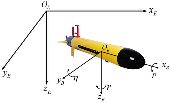
Figure 1. Coordinate system of UUV.

2.1. UUV Model

The earth-fixed frame $O_E-x_E{y}_E{z}_E$ and the body-fixed reference frame $O_B-x_B{y}_B{z}_B$ are employed to describe the motion of UUVs. The position and attitude of the UUV are defined as $\mathit{\eta }=[x,y,z,\phi ,\theta ,\psi {]}^{\mathrm{T}}\in {\mathbb{R}}^6$. $\mathit{v}=[u,v,w,p,q,r{]}^{\mathrm{T}}\in {\mathbb{R}}^6$ is the linear velocity and angular velocity of the UUV.

The kinematic transformation matrix from $O_B-x_B{y}_B{z}_B$ to $O_E-x_E{y}_E{z}_E$ coordinate system is represented as

$$\mathit{J}\left(\mathit{\eta }\right)=\left[\begin{array}{cc}{\mathit{J}}_1& 0_{3\times 3}\\ 0_{3\times 3}& {\mathit{J}}_2\end{array}\right]$$

(1)

where ${\mathit{J}}_1$ and ${\mathit{J}}_2$ are given by

$${\mathit{J}}_1=\left[\begin{array}{ccc}{c}_{\psi }{c}_{\theta }& -s_{\psi }{c}_{\phi }+c_{\psi }{s}_{\theta }{s}_{\phi }& s_{\psi }{s}_{\phi }+c_{\psi }{s}_{\theta }{c}_{\phi }\\ s_{\psi }{c}_{\theta }& c_{\psi }{c}_{\phi }+s_{\psi }{s}_{\theta }{s}_{\phi }& -c_{\psi }{s}_{\phi }+s_{\psi }{s}_{\theta }{c}_{\phi }\\ -s_{\theta }& s_{\phi }{c}_{\theta }& c_{\phi }{c}_{\theta }\end{array}\right]$$

(2)

and

$${\mathit{J}}_2\left({\mathit{\eta }}_2\right)={\displaystyle \frac{1}{c_{\theta }}}\left[\begin{array}{ccc}{c}_{\theta }& s_{\phi }{s}_{\theta }& c_{\phi }{s}_{\theta }\\ 0& c_{\phi }{c}_{\theta }& -s_{\phi }{c}_{\theta }\\ 0& s_{\phi }& c_{\phi }\end{array}\right].$$

(3)

Here $s_{(·)}$ and $c_{(·)}$ are short for $\sin (·)$ and $\cos (·)$.

Then the kinematic model is written as:

$$\dot{\mathit{\eta }}=\mathit{J}\left(\mathit{\eta }\right)\mathit{v}.$$

(4)

It is noteworthy that the kinematic model exhibits a singularity when the pitch angle $\theta =\pm {\displaystyle \frac{\pi }{2}}$. Therefore, $\theta$ is constrained within $(-\pi /2,+\pi /2)$.

The dynamic model is developed in a body-fixed frame $O_B-x_B{y}_B{z}_B$, with its origin $O_B$ coinciding with the center of buoyancy (CB). The origin $O_B$, is located at the vehicle’s CB. The dynamic equation of UUV can be expressed as

$$\mathit{M}\dot{\mathit{v}}+\mathit{C}\left(\mathit{v}\right)\mathit{v}+\mathit{D}\left(\mathit{v}\right)\mathit{v}+\mathit{g}\left(\mathit{\eta }\right)=\mathit{\tau }+{\mathit{\tau }}_d$$

(5)

where $\mathit{M}$, $\mathit{C}\left(\mathit{v}\right)$ and $\mathit{D}\left(\mathit{v}\right)$ are the inertia matrix, the Coriolis-centripetal matrix and the damping matrix, respectively. $\mathit{g}\left(\mathit{\eta }\right)$ represents the force/moment vector due to gravity and buoyancy in body-fixed frame. $\mathit{\tau }=[{\tau }_u,{\tau }_v,{\tau }_w,{\tau }_p,{\tau }_q,{\tau }_r{]}^{\mathrm{T}}$ denotes the control force and control torque vector. ${\mathit{\tau }}_d={\mathit{\tau }}_{\gamma }+{\mathit{\tau }}_{\delta }+{\mathit{\tau }}_{\varsigma }$ is the bounded external disturbance including the bounded external disturbance ${\mathit{\tau }}_{\gamma }$ with $\parallel {\mathit{\tau }}_{\gamma }\parallel \le \gamma$, the model uncertainties with $\parallel {\mathit{\tau }}_{\delta }\parallel \le \delta$ and the unmodeled dynamics and sensor noise ${\mathit{\tau }}_{\varsigma }$ with $\parallel {\mathit{\tau }}_{\varsigma }\parallel \le \varsigma$, where $\gamma$, $\delta$ and $\varsigma$ are positive constants.

According to the kinematic model (4) and the dynamic model (5), the motion model for UUV docking is expressed as

$$\dot{\mathit{x}}=\left[\begin{array}{c}\mathit{J}\left(\mathit{\eta }\right)\mathit{v}\\ {\mathit{M}}^{-1}\left(\mathit{\tau }+{\mathit{\tau }}_d-\mathit{C}\left(\mathit{v}\right)\mathit{v}-\mathit{D}\left(\mathit{v}\right)\mathit{v}-\mathit{g}\left(\mathit{\eta }\right)\right)\end{array}\right]=f\left({\mathit{x},\mathit{\tau },\mathit{\tau }}_d\right)$$

(6)

where $\mathit{x}={\left[{\mathit{\eta }}^{\mathrm{T}},{\mathit{v}}^{\mathrm{T}}\right]}^{\mathrm{T}}$ is the model state vector.

2.2. Gaussian Process-Based Model

Consider the UUV as a nonlinear discrete-time system, the significant model uncertainties and external disturbances lead to complex residual dynamics. In this work, GP regression is employed to capture these effects. As a non-parametric Bayesian method, GP excels at learning such unknown functions directly from data, providing a probabilistic estimate of the discrepancy between the nominal model and the true system behavior.

Discretize the complex nonlinear dynamic model (6) and the following form of discrete-time state space expression is obtained

$${\mathit{x}}_{k+1}=f\left({\mathit{x}}_k,{\mathit{\tau }}_k\right)+{\mathit{w}}_k$$

(7)

where k denotes the discrete index. ${\mathit{x}}_k\in {\mathbb{R}}^{12}$ is the state vector of the system and ${\mathit{\tau }}_k\in {\mathbb{R}}^6$ is the control input at discrete time k. The unknown function $f:{\mathbb{R}}^{12}\times {\mathbb{R}}^6\to {\mathbb{R}}^{12}$ represents the real but partially unknown nonlinear dynamic characteristics of the system. ${\mathit{w}}_k\sim \mathcal{N}\left(0,{\sigma }_w^2\right)$ is used to describe measurement noise and small random disturbances.

The state-input tuple ${\mathit{z}}_k={\left[\begin{array}{cc}{\mathit{x}}_k^{\mathrm{T}}& {\mathit{\tau }}_k^{\mathrm{T}}\end{array}\right]}^{\mathrm{T}}$ is defined as the input for the GP model. The system function $f\left({\mathit{z}}_k\right)$ is decomposed into a known nominal model $m\left({\mathit{z}}_k\right)$ and an unknown residual dynamic $d\left({\mathit{z}}_k\right)$, that is

$$f\left({\mathit{z}}_k\right)=m\left({\mathit{z}}_k\right)+d\left({\mathit{z}}_k\right).$$

(8)

We assume that the residual function follows a Gaussian process prior distribution as follows

$$d\left(\mathit{z}\right)\sim \mathcal{G}\mathcal{P}\left(0,k\left(\mathit{z},{\mathit{z}}^{\prime }\right)\right)$$

(9)

where the zero function is taken as its prior mean, and $k\left(\mathit{z},{\mathit{z}}^{\prime }\right)$ is the covariance function, which defines the correlation between different input points $\mathit{z}$ and ${\mathit{z}}^{\prime }$ their corresponding outputs. We choose the Square Exponential (SE) kernel function with infinite differentiability because it can effectively model smooth dynamic processes:

$$k\left(\mathit{z},{\mathit{z}}^{\prime }\right)={\sigma }_f^{2}exp\left(-{\displaystyle \frac{1}{2}}{\left(\mathit{z}-{\mathit{z}}^{\prime }\right)}^{\mathrm{T}}{\Lambda }^{-1}\left(\mathit{z}-{\mathit{z}}^{\prime }\right)\right)$$

(10)

where $\Lambda =\mathrm{diag}(l_1^2,\dots ,l_{18}^2)$ denotes a diagonal matrix containing feature length scales and ${\sigma }_f$ is GP signal variances. The selection of the SE kernel in (10) is driven by the physical characteristics of the UUV. The hydrodynamic forces and moments acting on the vehicle are physically smooth and continuous functions of the state and input. The SE kernel, with its infinite differentiability, effectively captures this underlying smoothness prior.

However, standard GP regression suffers from a significant computational burden. Define a dataset $\mathcal{D}=\left\{Z,Y\right\}$ containing sets of actual measurement data, where $Z={\left[{\mathit{z}}_1,\dots ,{\mathit{z}}_n\right]}^{\mathrm{T}}$ is the input vector and $Y={\left[y_1,\dots ,y_n\right]}^{\mathrm{T}}$ is the corresponding output vector. For the dataset $\mathcal{D}$, predictions require the inversion of an $n\times n$ covariance matrix, leading to a computational complexity of $\mathcal{O}\left(n^3\right)$ for training and $\mathcal{O}\left(n\right)$ for prediction. This complexity makes it prohibitive for real-time applications like MPC, where the model must be evaluated rapidly and the dataset may grow large.

To ensure computational tractability, we employ a sparse GP approximation. Sparse methods reduce complexity by summarizing the entire dataset using a smaller, representative set of $n_s$ inducing points, where $n_s\ll n$. We adopt the Subset of Regressors (SoR) approximation, which forms the basis for predictions on the selected active set of $n_s$ data points $\left\{Z_{n_s},Y_{n_s}\right\}\subseteq \mathcal{D}$. This approach reduces the training and prediction complexity to $\mathcal{O}\left(n{n}_s^2\right)$ and $\mathcal{O}\left(n_s\right)$, respectively, making it suitable for online implementation.

${\mathit{y}}_i={\mathit{x}}_{i+1}-m\left({\mathit{x}}_i,{\mathit{\tau }}_i\right)$ is calculated based on the difference between the actual measured state changes and the nominal model predictions. The hyperparameters $\theta =\left\{{\sigma }_f,\Lambda ,{\sigma }_w\right\}$ will be determined by maximizing the log marginal likelihood

$${\theta }^{\ast }=\underset{\theta }{\arg max}log\left(p\left(Y_{n_s}\left|Z_{n_s},\theta \right.\right)\right)$$

(11)

The training process involves determining the optimal hyperparameters $\theta =\{{\sigma }_f,\Lambda ,{\sigma }_w\}$ by maximizing the log marginal likelihood (11). We employ the Limited-memory Broyden–Fletcher–Goldfarb–Shanno optimization algorithm to solve this non-convex optimization problem efficiently. For the Sparse GP approximations, the locations of the inducing points $Z_{n_s}$ are initialized using K-means clustering on the training dataset to ensure a representative coverage of the input space.

Under the SoR framework, the predictive distribution for a new test input ${\mathit{z}}^{\ast }$ is conditioned only on this active set, rather than the full dataset. The joint distribution is approximated as

$$\left[\begin{array}{c}{Y}_{n_s}\\ d\left({\mathit{z}}^{\ast }\right)\end{array}\right]\sim \mathcal{N}\left(0,\left[\begin{array}{cc}K\left(Z_{n_s},Z_{n_s}\right)+{\sigma }_w^{2}I& K{\left({\mathit{z}}^{\ast },Z_{n_s}\right)}^{\mathrm{T}}\\ K\left({\mathit{z}}^{\ast },Z_{n_s}\right)& K\left({\mathit{z}}^{\ast },{\mathit{z}}^{\ast }\right)\end{array}\right]\right)$$

(12)

where $K\left(Z_{n_s},Z_{n_s}\right)=\left[k\left({\mathit{z}}_i,{\mathit{z}}_j\right)\right]\in {\mathbb{R}}^{n_s\times n_s}$ is the covariance matrix, where $i,j\in {\mathbb{N}}_1^{n_s}$. The covariance vector is $K\left({\mathit{z}}^{\ast },Z_{n_s}\right)={\left[k\left({\mathit{z}}^{\ast },{\mathit{z}}_1\right),\dots ,k\left({\mathit{z}}^{\ast },{\mathit{z}}_{n_s}\right)\right]}^{\mathrm{T}}$. By conditioning the joint distribution, given the dataset and a test input ${\mathit{z}}^{\ast }$, the resulting posterior distribution of the residual term follows a Gaussian distribution:

$$d\left({\mathit{z}}^{\ast }\right)\left|\mathcal{D},\theta \right.\approx d\left({\mathit{z}}^{\ast }\right)\left|\left\{Z_{n_s},Y_{n_s}\right\},\theta \right.\sim \mathcal{N}\left({\mu }_d\left({\mathit{z}}^{\ast }\right),{\sigma }_d^2\left({\mathit{z}}^{\ast }\right)\right)$$

(13)

The posterior mean and posterior variance are updated through

$${\mu }_d\left({\mathit{z}}^{\ast }\right)=K\left({\mathit{z}}^{\ast },Z_{n_s}\right){\left[K\left(Z_{n_s},Z_{n_s}\right)+{\sigma }_w^{2}I\right]}^{-1}{Y}_{n_s}$$

(14)

and

$${\sigma }_d^2\left({\mathit{z}}^{\ast }\right)=K\left({\mathit{z}}^{\ast },{\mathit{z}}^{\ast }\right)-K\left({\mathit{z}}^{\ast },Z_{n_s}\right){\left[K\left(Z_{n_s},Z_{n_s}\right)+{\sigma }_w^{2}I\right]}^{-1}K{\left({\mathit{z}}^{\ast },Z_{n_s}\right)}^{\mathrm{T}}.$$

(15)

The term $\alpha ={\left[K\left(Z_{n_s},Z_{n_s}\right)+{\sigma }_w^{2}I\right]}^{-1}{Y}_{n_s}$ can be pre-computed after training, making online prediction of the mean extremely fast, requiring only the computation of the covariance vector $K\left({\mathit{z}}^{\ast },Z_{n_s}\right)$. The final GP enhanced model for UUV, which is embedded into the MPC framework, is thus formulated as

$${\widehat{\mathit{x}}}_{k+1}=f\left({\widehat{\mathit{x}}}_k,{\mathit{\tau }}_k\right)=m\left({\widehat{\mathit{x}}}_k,{\mathit{\tau }}_k\right)+{\mu }_d\left({\widehat{\mathit{x}}}_k,{\mathit{\tau }}_k\right)$$

(16)

This model not only provides accurate estimation of the next state, but also quantifies the uncertainty predicted at that point through posterior variance ${\sigma }_d^2\left({\mathit{z}}^{\ast }\right)$.

It is important to acknowledge the sensitivity of the controller’s performance to the quality and scope of this training data. The GP regression provides accurate mean predictions and low variance estimates primarily within the support of the training distribution. When the UUV operates in regions significantly distinct from the training data, the GP posterior variance ${\sigma }_d^2\left(z^{\ast }\right)$ increases, reflecting higher uncertainty. While the MPC optimizes conservatively against this uncertainty, extreme extrapolation can lead to substantial prediction errors that exceed the controller’s compensatory capacity, resulting in performance degradation. Therefore, the adopted Mixed Excitation Strategy is critical, as it maximizes the coverage of the state space to minimize the risks associated with operating outside the training distribution.

To ensure the GP model generalizes well across the operational envelope, a Mixed Excitation Strategy is adopted for data collection. The training dataset $\mathcal{D}$ is constructed using two types of trajectories:

• Nominal Operation Data (75%): Generated from closed-loop control simulations using the nominal model. This data ensures high prediction accuracy in the regions where the UUV operates most frequently.
• Random Excitation Data (25%): Generated by applying random amplitude and frequency inputs (Generalized Binary Noise or Chirp signals) to the open-loop system. This data enhances the exploration of the state space and captures the system response at the boundaries of the dynamics, satisfying the persistent excitation condition.

Remark 1.

The relative order of the actual UUV system is $r=2$. GP directly provides an affine approximation of $\mathit{x}$ over $\mathit{\tau }$, so the input-output relationship can be regarded as a relative order $r=1$. This approach reduces controller complexity and avoids redundant terminal structure design.

2.3. Problem Statement

The docking process of UUV is demonstrated in Figure 2. During the terminal guidance phase of UUV docking, ensuring that the position and posture of the UUV always remain within a safety corridor that tightens with distance reduction is the key to ensuring successful docking. The goal of this work is to guide the UUV through a constrained safety corridor to successfully achieve autonomous docking.

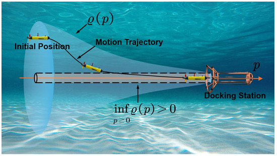
Figure 2. UUV docking diagram.

The ultimate control objective is to drive the UUV to accomplish autonomous docking with high precision. In the context of this study, high precision is characterized by achieving sub-meter position accuracy and sub-degree heading alignment relative to the docking station, ensuring the vehicle can be reliably captured by the mechanical interface.

3. Docking Control Based on GP-Based Funnel MPC

This section details a GP-based Funnel MPC for precise UUV docking, which frames the task as a constrained optimization problem using a GP relative error dynamics model as shown in Figure 3. By transforming state constraints into a cost function penalty, the method enforces a strict funnel boundary on the error, thereby circumventing the numerical issues of hard constraints.

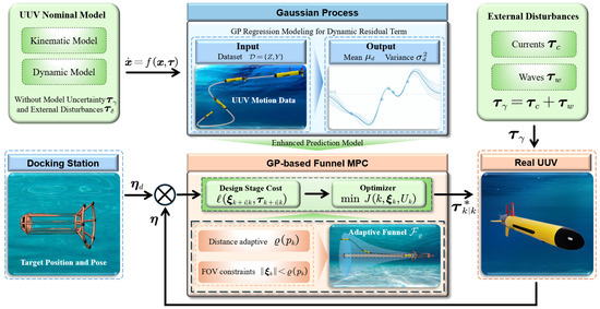
Figure 3. MPC control framework.

Firstly, a Docking Funnel that adapts to contraction with distance is designed to ensure that pose errors during the docking process always remain within a predetermined, time-varying safety boundary. Furthermore, embedding this funnel constraint into the cost function, an MPC problem without terminal constraints is constructed to calculate the optimal control input online [38].

3.1. Adaptive Funnel Design Considering FOV Constraints

The dynamics of the system can be predicted using the GP model established in Section 2.2. The position of the docking station is measured by using an acoustic or optical positioning system, which is defined as ${\mathit{\eta }}_d$. Let the output error be ${\mathit{\xi }}_k={\mathit{\eta }}_k-{\mathit{\eta }}_{d,k}\in \mathbb{Z}$, where $\mathbb{Z}$ is the state error constraint and ${\mathit{\eta }}_{d,k}$ is the reference state at time k. Due to the direct learning of GP from input ${\mathit{\tau }}_k$ to state ${\mathit{x}}_{k+1}$, resulting in a relative order $r=1$, we adopt a Funnel MPC design to predict nonlinear dynamics around a reference trajectory at each sampling time k:

$$\begin{array}{cc}{\mathit{\xi }}_{k+i\left|k\right.}={\mathit{C}\widehat{\mathit{x}}}_{k+i\left|k\right.}-{\mathit{\eta }}_{d,k+i\left|k\right.}& i\in {\mathbb{N}}_0^{N-1}\end{array}$$

(17)

where $\mathit{C}=\left[{\mathit{I}}_{5\times 5},0_{5\times 5}\right]$ is the output matrix. ${\mathit{\xi }}_{k+i|k}$ is the predicted value of the state error at the current time k for the future time $k+i$. The future state error of the system in the predicted horizon N is predicted by the following equation:

$${\widehat{\mathit{x}}}_{k+i+1\left|k\right.}=m\left({\widehat{\mathit{x}}}_{k+i\left|k\right.},{\mathit{\tau }}_{k+i\left|k\right.}\right)+{\mu }_d\left({\widehat{\mathit{x}}}_{k+i\left|k\right.},{\mathit{\tau }}_{k+i\left|k\right.}\right)$$

(18)

where ${\widehat{\mathit{x}}}_{k\left|k\right.}={\mathit{x}}_k$ and ${\mathit{\tau }}_{k+i|k}\in \mathbb{U}$ is the control input with the predicted horizon for $i\in {\mathbb{N}}_0^{N-1}$, where $\mathbb{U}$ is the control constraint.

To satisfy the FOV constraints during terminal docking maneuvers, a docking funnel framework was developed. This approach guides the UUV by placing predefined bounds on its relative pose. It serves as a prescribed performance boundary where the allowable error margin is dynamically scaled based on the UUV’s proximity to the dock. Let the path deviation error at the initial time be $p_0$. And at the $k_{th}$ moment, the path deviation error is defined as

$$p_k=∥\left[\begin{array}{c}{x}_k\\ y_k\\ z_k\end{array}\right]-\left[\begin{array}{c}{x}_{d,k}\\ y_{d,k}\\ z_{d,k}\end{array}\right]∥.$$

(19)

Define function category $\mathcal{G}$ as [39]:

$$\mathcal{G}:=\left\{\varrho \in W^{1,\infty }\left({\mathbb{R}}_{\ge 0},\mathbb{R}\right)\left|\begin{array}{c}\underset{p\ge 0}{\inf }\varrho \left(p\right)>0\\ \exists \alpha ,\beta >0\forall k\in {\mathbb{R}}_{\ge 0}:\\ \dot{\varrho }\left(p_k\right)\ge -\alpha \varrho \left(p_k\right)+\beta \end{array}\right.\right\}$$

(20)

A monotonically decreasing function $\varrho \left(p_k\right)\in \mathcal{G}$ is used as the funnel boundary to ensure that the allowable error boundary tightens as the path deviation error decreases. Therefore, an Exponential Funnel is selected as

$$\varrho \left(p_k\right)=\left({\varrho }_0-{\varrho }_f\right)exp\left(-ϵ\left(p_0-p_k\right)\right)+{\varrho }_f$$

(21)

where ${\varrho }_0$ and ${\varrho }_f$ denote maximum error norm allowed at initial distance and final docking moment, respectively. $ϵ$ is the adjustment parameter that controls the contraction rate of the funnel. The design of the performance funnel $\varrho \left(p_k\right)$ is physically motivated by the Field of View (FOV) constraints of the onboard sensors. Mathematically, the path deviation $p_k$ serves as a scalar indicator of the docking progress, derived directly from the system state $x_k$ via the relative position vector. The exponential decay form in (21) is selected to strictly envelope the sensor’s conical visible region. As the UUV approaches the station (i.e., $p_k\to 0$), the allowable lateral error $\varrho \left(p_k\right)$ must shrink continuously to ensure the docking station remains observable. The specific relationship is constructed such that if the state error $\parallel {\xi }_k\parallel$ satisfies $\parallel {\xi }_k\parallel <\varrho \left(p_k\right)$, the target is guaranteed to be within the sensor’s FOV.

The error should satisfy $\parallel {\mathit{\xi }}_k\parallel <\varrho \left(p_k\right)$, that is, they should be ensured within the performance funnel as follows

$${\mathcal{F}}_{\varrho }=\left\{\left(p,\mathit{\xi }\right)\in {\mathbb{R}}_{\ge 0}\times {\mathbb{R}}^n\left|\parallel {\mathit{\xi }}_k\parallel <\varrho \left(p_k\right),\forall k\ge 0\right.\right\}.$$

(22)

To ensure that the state error ${\mathit{\xi }}_k$ remains within set ${\mathcal{F}}_{\varrho }$, the state of system (6) should be guaranteed to satisfy

$${\mathit{x}}_k\in {\mathcal{H}}_k^{\varrho }=\left\{{\mathit{x}}_k\in {\mathbb{R}}^{12}\left|\parallel {\mathit{Cx}}_k-{\mathit{\eta }}_{d,k}\parallel <\varrho \left(p_k\right)\right.\right\}.$$

(23)

Assumption 1.

At the initial time $k=0$, the initial state ${\mathit{x}}_0$ of the UUV strictly lies within a contraction region of the performance funnel as follows

$${\mathit{x}}_0\in {\mathcal{H}}_0^{\varrho }$$

(24)

Remark 2.

In practical engineering applications, Assumption 1 serves a dual purpose. First, it defines the entry condition for the terminal docking phase within a hierarchical control architecture. A long-range navigation controller guides the UUV to the rendezvous point, and the proposed GP-based Funnel MPC activates only when the UUV enters the capture region defined by $\varrho \left(p_0\right)$. Second, it establishes the trigger for recovery protocols. If this assumption is violated during operation, the barrier cost function becomes undefined. To ensure robustness, a hybrid recovery strategy is required: the system temporarily switches to a fallback controller to steer the UUV back into the safe envelope. The high-precision Funnel MPC is then re-activated only once the state error re-enters the funnel defined by $\varrho \left(p_k\right)$, ensuring continuous and safe operation.

3.2. The Design of MPC Controller

In Section 3.1, we defined a distance-adaptive funnel. However, directly incorporating the time-varying error constraint as hard constraints into the optimization problem will greatly increase the difficulty of solving. Inspired by Funnel MPC [40], we incorporate the constraint into the optimization objective by designing a stage cost function similar to the Barrier Function.

Considering the tracking error weight matrix $\mathit{Q}$ and the control input weight matrix $\mathit{R}$, the stage cost is defined as

$$\ell ({\mathit{\xi }}_{k+i|k},{\mathit{\tau }}_{k+i|k})={\displaystyle \frac{{\parallel {\mathit{\xi }}_{k+i|k}\parallel }_{\mathit{Q}}^2}{{\varrho }^2\left(p_k\right)-{\parallel {\mathit{\xi }}_{k+i|k}\parallel }_{\mathit{Q}}^2}}+{\parallel {\mathit{\tau }}_{k+i|k}\parallel }_{\mathit{R}}^2$$

(25)

The stage cost function (25) employs a barrier-type formulation. The term ${\varrho }^2\left(p_k\right)-{\parallel {\xi }_{k+i|k}\parallel }_Q^2$ in the denominator acts as a virtual potential field. As the weighted error approaches the funnel boundary $\varrho \left(p_k\right)$, the denominator tends to zero, causing the cost to approach infinity. This mechanism forces the optimizer to find control actions that strictly keep the predicted trajectory within the interior of the funnel, thereby enforcing the safety constraint without using hard numerical constraints that might cause feasibility issues.

The selection of the weighting matrices $\mathit{Q}$ and $\mathit{R}$ follows a two-step tuning procedure. First, we apply Bryson’s rule for initialization, where the diagonal elements are set inversely proportional to the square of the maximum acceptable values for each state and input component. Second, these weights are fine-tuned iteratively through simulation. The error weight $\mathit{Q}$ is increased to prioritize tracking accuracy closer to the dock, while $\mathit{R}$ is adjusted to prevent actuator saturation and ensure smooth control signals, avoiding high-frequency chattering.

At each sampling time k, the controller obtains the (sub)optimal control input sequence $U_k^{\ast }=\{{\mathit{\tau }}_{k|k}^{\ast },\dots ,{\mathit{\tau }}_{k+N-1|k}^{\ast }\}$ by solving a finite horizon optimal control problem. Considering the prediction horizon N of the controller, the cost function of the MPC controller is defined as

$$J(k,{\mathit{\xi }}_k,U_k)=\sum _{i=0}^{N-1}\ell ({\mathit{\xi }}_{k+i|k},{\mathit{\tau }}_{k+i|k})$$

(26)

In addition to the funnel-based error constraints, the MPC formulation must explicitly incorporate input constraints to ensure feasibility and safety of the docking maneuver. The terminal cost is defined as a control Lyapunov function $V_f\left(\mathit{\xi }\right)={\mathit{\xi }}^{\mathrm{T}}\mathit{P}\mathit{\xi }$ to ensure stability, where $\mathit{P}$ is a positive definite matrix. Correspondingly, the terminal region $\Omega =\{\mathit{\xi }\in {\mathbb{R}}^{12}|V_f\left(\mathit{\xi }\right)\le \varpi \}$ is a compact set containing the origin, where $\varpi$ is a sufficiently small positive constant.

The control input ${\mathit{\tau }}_k$, which corresponds to the control forces and torques, is restricted by actuator limitations. Specifically, the input control constraint $\mathbb{U}$ is expressed as $\mathbb{U}=\{\mathit{\tau }\in {\mathbb{R}}^6|{\mathit{\tau }}_{min}\le \mathit{\tau }\le {\mathit{\tau }}_{max}\}$, where ${\mathit{\tau }}_{min}$ and ${\mathit{\tau }}_{max}$ are determined by the saturation bounds of the UUV thrusters and control surfaces. These constraints prevent infeasible control efforts and protect the actuators from overloading. The input control constraint $\mathbb{U}$ are defined by a convex polyhedron, which can be expressed as a set of linear inequalities, i.e.,

$$\mathbb{U}=\left\{\mathit{\tau }\in {\mathbb{R}}^6|{\mathit{C}}_{\tau }\mathit{\tau }\le \Delta \right\}$$

(27)

where ${\mathit{C}}_{\tau }$ and $\Delta$ are constraint matrix and vector describing the constraint region. This property guarantees the existence of a local state feedback gain matrix $\mathit{K}$ that renders a terminal set $\Omega$ and an invariant region for the closed-loop system, while satisfying all constraints for any state within $\Omega$.

In contrast, the proposed GP-based Funnel MPC framework sidesteps this requirement for terminal terms. The feasibility of the controller is inherently guaranteed by the construction of the funnel itself, without resorting to an explicit terminal cost or terminal constraint. The optimization problem is formulated to find a control sequence that keeps the state trajectory within the predefined, time-varying funnel boundary. Therefore, the optimization problem is constructed as follows:

At each time k, given the system state ${\mathit{x}}_k$ and the state of the docking station ${\mathit{\eta }}_{d,k}$, the GP-based Funnel MPC problem is described as:

$$\mathcal{P}:\begin{array}{cc}{\displaystyle \underset{U_k^{\ast }}{min}}& J(k,{\mathit{\xi }}_k,U_k)\end{array}$$

(28)

s.t.

$${\mathit{\xi }}_{k|k}={\mathit{\xi }}_k$$

(29)

$$\begin{array}{cc}{\widehat{\mathit{x}}}_{k+i+1|k}=f({\widehat{\mathit{x}}}_{k+i|k},{\mathit{\tau }}_{k+i|k}),& i\in {\mathbb{N}}_0^{N-1}\end{array}$$

(30)

$$\begin{array}{cc}{\mathit{\xi }}_{k+i|k}\in \mathbb{Z},& i\in {\mathbb{N}}_0^{N-1}\end{array}$$

(31)

$$\begin{array}{cc}{\mathit{\tau }}_{k+i|k}\in \mathbb{U},& i\in {\mathbb{N}}_0^{N-1}\end{array}$$

(32)

By solving $\mathcal{P}$ above, the control efforts for the docking control are obtained and the first element ${\mathit{\tau }}_{k|k}^{\ast }$ of the optimization sequence $U_k^{\ast }$ is applied to the UUV system.

Remark 3.

If an explicit $r=2$ design is desired, the auxiliary error needs to be constructed, and the form of the stage cost in (25) needs to be improved. The feasibility of the problem is still guaranteed without terminal conditions. We do not adopt this here to keep the controller minimal for the UUV case.

3.3. Theoretical Analysis of Synergy and Robustness

In this subsection, we analyze the synergistic mechanism between the GP regression and the Funnel MPC, and theoretically demonstrate how this integration enhances the system’s robustness and safety compared to traditional methods.

The core challenge in UUV docking is satisfying the stringent state constraints imposed by the funnel ${\mathcal{F}}_{\varrho }$ in the presence of significant model uncertainties. For a standard Funnel MPC without learning, the prediction model relies solely on the nominal dynamics $m(x_k,{\tau }_k)$. The prediction error grows rapidly with the horizon steps due to the unmodeled residual dynamics $d(x_k,{\tau }_k)$. Mathematically, if the magnitude of the unmodeled dynamics is bounded, the worst-case prediction error accumulates. In the terminal guidance phase, the funnel boundary $\varrho \left(p_k\right)$ shrinks towards a small value ${\varrho }_f$. If the accumulated prediction uncertainty exceeds the available safety margin, i.e., the width of the funnel, the optimization problem $\mathcal{P}$ in (28) becomes infeasible, leading to control failure.

The incorporation of GP establishes a synergistic loop that restores feasibility. By utilizing the posterior mean ${\mu }_d\left(z_k\right)$ to compensate for the nominal model in (16), the significant deterministic component of the model mismatch is removed. The dynamics perceived by the MPC controller shifts from

$$\begin{array}{c}{x}_{k+1}=m(x_k,{\tau }_k)+d\left(z_k\right)\end{array}$$

(33)

to

$$\begin{array}{c}{x}_{k+1}=m(x_k,{\tau }_k)+{\mu }_d\left(z_k\right)+w_k^{\prime }\end{array}$$

(34)

where $w_k^{\prime }$ represents the residual aleatoric uncertainty, which follows a zero-mean Gaussian distribution with a variance of ${\sigma }_d^2\left(z_k\right)$. This transformation significantly narrows the spread of predicted state trajectories, ensuring that they can feasibly fit within the tightening funnel constraint ${\mathcal{H}}_k^{\varrho }$ defined in (23), thus guaranteeing the solvability of the optimization problem during close-range maneuvers.

Traditional robust control strategies, such as Tube-based MPC, typically address uncertainties by defining a robust positively invariant set around the nominal trajectory. This relies on a fixed, worst-case assumption of the disturbance, i.e., $d\left(z\right)\in \mathbb{W}$, where $\mathbb{W}=\{w\mid \parallel w\parallel \le \overline{w}\}$. In the complex underwater environment, determining a tight bound $\overline{w}$ is difficult. To ensure safety, one must choose a conservative $\overline{w}$ that covers all possible currents and hydrodynamic effects. However, a large $\overline{w}$ results in a "fat" tube. In the docking scenario, as the UUV approaches the station, the allowable error corridor (the funnel) becomes extremely narrow. If the width of the invariant tube defined by the worst-case robust MPC is larger than the terminal funnel width ${\varrho }_f$, the controller will fail to find a solution.

In contrast, our proposed method leverages the state-dependent nature of the GP uncertainty. The GP provides a local confidence ellipsoid based on the variance ${\sigma }_d^2\left(z_k\right)$, which adapts to the current state and data density. In regions where the model is well-known or the disturbances are locally smooth, the uncertainty bound provided by GP is significantly smaller than the global worst-case bound $\overline{w}$ used in Tube MPC. This adaptability allows the “effective tube” of our controller to shrink dynamically, enabling the UUV to navigate through the narrow bottleneck of the docking funnel without violating constraints, a performance level that traditional fixed-tube robust MPC cannot achieve.

While deterministic safety is challenging to prove with stochastic learning models, the proposed framework offers a probabilistic safety guarantee. Based on the GP posterior distribution, the residual dynamics fall within the confidence interval ${\mu }_d\left(z_k\right)\pm 2{\sigma }_d\left(z_k\right)$ with a probability of approximately 95%. By integrating the funnel constraint into the cost function via the barrier-like term in (25), the controller is penalized heavily as the state approaches the boundary $\varrho \left(p_k\right)$. Given that the GP-compensated prediction error is small, there exists a control input $\tau \in \mathbb{U}$ such that the predicted state plus the confidence bound remains within the funnel:

$$\begin{array}{c}\parallel {\xi }_{k+1}\parallel +2{\sigma }_d({\widehat{x}}_k,{\tau }_k)<\varrho \left(p_{k+1}\right)\end{array}$$

(35)

This condition implies that the system states are recursively feasible with high probability.

4. Numerical Simulation

Comparative numerical simulation is implemented in this section to evaluate the effectiveness of the proposed MPC scheme. The simulation is conducted by Matlab/Simulink on a Ryzen 7 7840HS/32 GB DDR5. To provide a benchmark for performance evaluation, a conventional MPC is introduced for comparative analysis. The nonlinear programming problem is solved using the IPOPT solver. Parametric model mismatches and external environmental perturbations are incorporated into the simulation to verify the resilience of the control scheme.

4.1. Parameter Selection

The parameters of the UUV nominal model are adopted from [41]. The sampling time is set to $T=0.02$ s (50 Hz) to sufficiently capture the fast dynamics of the UUV thrusters and hydrodynamic responses. The prediction horizon is selected as $N=20$. This provides a sufficient look-ahead window (0.4 s) to anticipate dynamic changes while keeping the optimization problem computationally tractable for real-time solving.

The initial state of UUV is ${\mathit{x}}_0={\left[{\mathit{\eta }}_0^{\mathrm{T}},{\mathit{v}}_0^{\mathrm{T}}\right]}^{\mathrm{T}}$, where the initial position and velocity are ${\mathit{\eta }}_0={\left[-50,-6,6,0,0,0\right]}^{\mathrm{T}}$ and ${\mathit{v}}_0=0_{6\times 1}$. The docking station position is ${\mathit{\eta }}_d=0_{6\times 1}$. The state error and the control input weight matrix of the controller are designed as

$$\mathit{Q}=\mathrm{diag}\left([1.5e4,1.5e4,1.5e4,1e4,1e4,1e4,1e5,1e6,8e5,8e4,8e4,8e4]\right)$$

(36)

and

$$\mathit{R}=\mathrm{diag}\left([5,10,10,10,10,10]\right).$$

(37)

The weighting matrices Q and R are tuned based on Bryson’s rule to normalize the different scales of state variables (positions in meters vs. angles in radians). Specifically, larger weights are assigned to position errors ($x,y,z$) to prioritize collision avoidance and docking accuracy, while the input weights R are set to penalize excessive energy consumption and prevent actuator saturation.

The control input is constrained by ${\mathit{\tau }}_{min}\le \mathit{\tau }\le {\mathit{\tau }}_{max}$, where ${\mathit{\tau }}_{max}$ and ${\mathit{\tau }}_{min}$ are upper and lower bounds, defined as

$$\left\{\begin{array}{cc}\hfill {\mathit{\tau }}_{max}& ={\left[100,30,30,30,30,30\right]}^{\mathrm{T}}\hfill \\ \hfill {\mathit{\tau }}_{min}& ={\left[0,-30,-30,-30,-30,-30\right]}^{\mathrm{T}}\hfill \end{array}\right.$$

(38)

Considering the weight matrix and a certain safety margin, the maximum error norms allowed at the initial distance and final docking time in (21) are designed as ${\varrho }_0=19516$ and ${\varrho }_f=1$. The funnel contraction rate is defined as $ϵ=0.04$. Under the above parameters, Assumption 1 is satisfied, and the funnel function is represented as

$$\varrho \left(p_k\right)=19506e^{-0.04\left(p_0-p_k\right)}+1.$$

(39)

The funnel parameters are derived from the physical mission constraints. ${\varrho }_0$ is set to enclose the initial maximum deviation. Crucially, the terminal radius ${\varrho }_f=1m$ is determined by the physical aperture size of the docking station to ensure safe entry. The contraction rate $ϵ=0.04$ is empirically selected to define a convergence profile that is dynamically feasible given the UUV’s maximum velocity and acceleration limits.

The training dataset $\mathcal{D}$ for GP consists of a mixed dataset. 75% of the dataset consists of closed-loop trajectories of NMPC controllers under various random initial conditions. In addition, to enhance the exploratory nature of the model, an additional 25% of the dataset consists of randomly controlled inputs and their corresponding system outputs, ensuring a more comprehensive coverage of the state space.

The external disturbances ${\mathit{\tau }}_{\gamma }$ comprised a constant ocean current disturbance ${\mathit{\tau }}_c$ and persistent wind/wave disturbance ${\mathit{\tau }}_w$, represented as

$${\mathit{\tau }}_{\gamma }={\mathit{\tau }}_c+{\mathit{\tau }}_w$$

(40)

To emulate persistent environmental loads disturbance ${\mathit{\tau }}_w$, the constant forces and moments are applied. A constant disturbance force vector ${\mathit{F}}_d={\left[10,5,5\right]}^{\mathrm{T}}$ N is defined in the earth-fixed frame and a constant disturbance moment vector ${\mathit{M}}_d={\left[3,3,3\right]}^{\mathrm{T}}$ Nm is applied directly in the body-fixed frame. The current disturbance ${\mathit{\tau }}_c$ is modeled as a constant, irrotational flow field acting exclusively in the horizontal plane of the earth-fixed frame. The velocity vector of the current is defined with a constant magnitude of 0.3 m/s and a fixed direction of $\pi /3$ rad. The current hydrodynamic effect is calculated based on the relative velocity between the UUV and the water.

To evaluate the controller’s robustness against modeling inaccuracies, a 15% mismatch is introduced between the nominal model used for MPC prediction and the plant model used for simulating the UUV’s dynamics. This is achieved by perturbing the hydrodynamic coefficients of the plant model. A zero-mean Gaussian white noise vector is employed to characterize both sensor noise and high-frequency unmodeled dynamics. The standard deviations for the force and moment components are set to $\varsigma ={\left[0.5,0.5,0.5,0.2,0.2,0.2\right]}^{\mathrm{T}}$. Finally, the external disturbances are caused by the external disturbances and model uncertainties as follows

$${\mathit{\tau }}_d={\mathit{\tau }}_{\gamma }+{\mathit{\tau }}_{\delta }+\varsigma$$

(41)

4.2. Performance of GP Model

The performance of the trained GP in modeling the system dynamics, and the resulting improvement over the nominal model, are presented in Figure 4, Figure 5 and Figure 6.

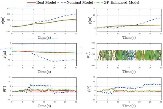
Figure 4. Comparison of Pose Components.

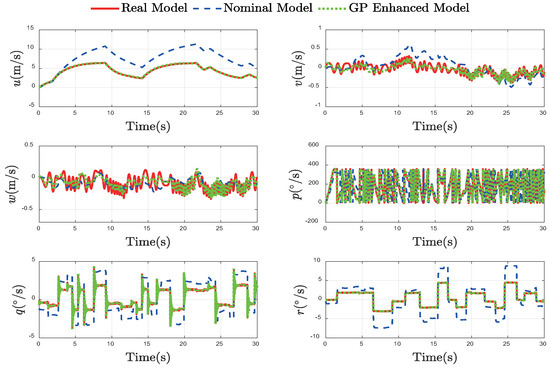
Figure 5. Comparison of Velocity Components.

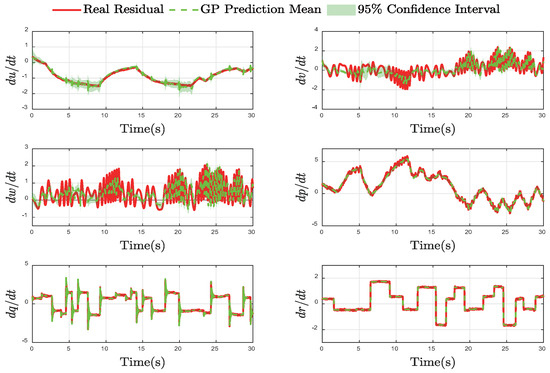
Figure 6. GP Residual with 95% Confidence Interval.

The benefits of this accurate residual modeling are demonstrated in the prediction of the system’s velocity and pose states, presented in Figure 4 and Figure 5, respectively. This velocity tracking is critical as it directly prevents the accumulation of integration errors over time. Consequently, at the pose level, the GP-enhanced model’s predicted trajectory remains closely aligned with the vehicle’s true path and orientation. This stands in sharp contrast to the nominal model’s pose prediction, which diverges dramatically, validating our method’s reliability for robust state estimation.

Figure 6 presents the core validation of the learning component, illustrating the GP’s ability to approximate the true residual dynamics. It is evident that the GP prediction mean tracks the true residual across all six degrees of freedom, including both low-frequency drifts and high-frequency variations. Furthermore, the true residual consistently lies within the 95% confidence bounds, indicating that the GP not only learns the system’s unmodeled dynamics but also provides a measure of its own predictive uncertainty. This result confirms that the GP has captured the underlying structure of the model–plant mismatch.

4.3. Comparative Docking Results

The comparative results of the docking task under the conventional MPC without disturbance, the conventional MPC with disturbance and the proposed method are presented in Figure 7, Figure 8, Figure 9, Figure 10, Figure 11 and Figure 12.

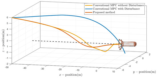
Figure 7. Docking Trajectories.

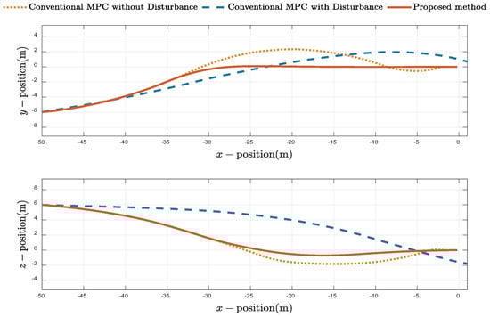
Figure 8. 2D projections of the UUV docking trajectories.

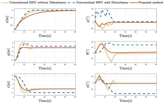
Figure 9. Comparison of Position and Attitude States.

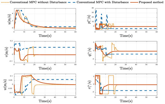
Figure 10. Comparison of Velocity States.

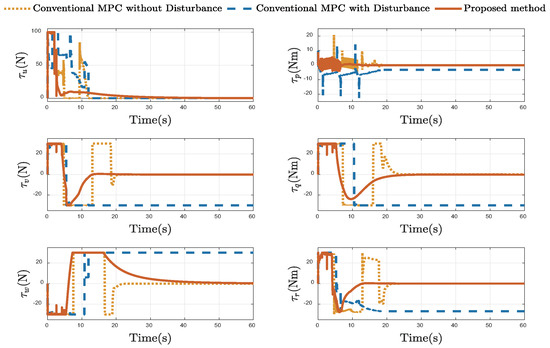
Figure 11. Comparison of Control Inputs.

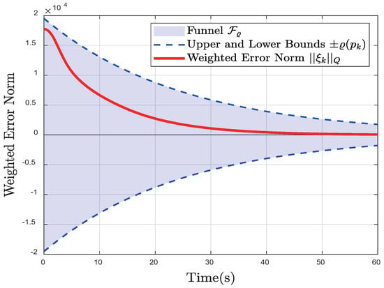
Figure 12. Funnel Visualization of Path Deviation Error.

Figure 7 and Figure 8 illustrate the 3D docking trajectories to compare the performance of the proposed method against a conventional MPC. Under ideal disturbance-free conditions, the conventional MPC successfully reaches the station, establishing a performance baseline. However, when external disturbances are introduced, the same conventional controller fails, exhibiting significant deviation and completely missing the docking station. This demonstrates its lack of robustness. Under the same disturbance conditions, the proposed MPC effectively compensates for the disturbances, guiding the UUV to a precise and successful docking.

Figure 9 provides a detailed comparison of the UUV’s position and attitude states with different control method. The conventional MPC, while effective in the disturbance-free baseline scenario, fails when disturbances are introduced. In contrast, the proposed method demonstrates exceptional performance. Its response curves for both position and attitude closely track the ideal values, highlighting its effective disturbance rejection capabilities.

Figure 10 displays the time evolution of the UUV’s linear and angular velocities. The results highlight the robustness of the proposed method. The conventional MPC under disturbance generates oscillatory control actions, particularly visible in the chattering-like behavior of the angular rates, and its linear velocities fail to settle at zero. The proposed method produces smooth velocity profiles that converge to zero, closely mimicking the ideal baseline. This demonstrates the controller’s ability to maintain stability and execute the maneuver efficiently despite external disturbances.

The control input profiles in Figure 11 provide a clear distinction between the two methods’ practical viability. The conventional MPC’s unstable and chattering inputs highlight its failure to handle disturbances robustly. The proposed method generates smooth and continuous control inputs. It effectively calculates the necessary actuation to reject disturbances without inducing oscillations, demonstrating robustness and control efficiency suitable for practical implementation.

The evolution of the weighted path deviation error norm is shown in Figure 12. As depicted, the system’s weighted error norm is strictly maintained within the predefined performance funnel. The error norm exhibits a smooth and monotonic convergence towards zero, indicating the good stability and tracking precision of the closed-loop system. This result validates the effectiveness of the control framework, which systematically guarantees safety and task performance by integrating the funnel constraint into the cost function without relying on terminal constraints.

The quantitative performance metrics are summarized in Table 1. Under external disturbances, the Conventional MPC exhibits large deviations ($2.85$ m position error) and fails to dock. Conversely, the proposed method effectively rejects disturbances, achieving a high terminal precision of $0.08$ m and $0.{26}^{\circ }$. Furthermore, the average computational time is reduced to $28.34$ ms, validating the method’s superior robustness and computational efficiency for real-time implementation.

Table 1. Quantitative performance comparison.

Metric	Conv. MPC (No Dist.)	Conv. MPC (With Dist.)	Proposed Method
Docking Status	Success	Failure	Success
Terminal Pos. Error (m)	0.05	2.85	0.08
Terminal Heading Error (°)	0.35	15.20	0.26
Avg. Computational Time (ms)	57.23	51.47	28.34

5. Conclusions

In this paper, a GP-based Funnel MPC strategy is introduced for UUV docking under conditions of parametric uncertainty and environmental loads. The integration of a GP model allows for the learning of residual dynamics, which effectively compensates for unmodeled components and significantly boosts prediction accuracy. Furthermore, a distance-adaptive performance funnel is designed and integrated into the MPC cost function to enforce prescribed, time-varying constraints on the state error. This approach systematically guarantees that the docking target remains observable without the computational complexity associated with terminal constraints.

Numerical simulations validated the effectiveness of the proposed framework. The results demonstrated that the controller successfully maintains the system error within the predefined funnel boundaries while ensuring smooth convergence. In comparative analyses under disturbance conditions, the proposed method achieved precise and robust docking, whereas conventional MPC failed, thus confirming the performance and viability of the proposed control strategy.

Despite these promising results, certain limitations remain. The current validation relies on numerical simulations which, although incorporating disturbances, model them primarily as steady currents and persistent forces. Consequently, the system’s performance under highly dynamic, time-varying, and turbulent sea states remains an open question. Furthermore, the simulation cannot fully replicate real-world complexities such as acoustic multipath effects and non-Gaussian sensor noise. Additionally, the framework currently focuses on open-water docking without dynamic obstacle avoidance. Finally, deploying the learning algorithm on resource-constrained embedded hardware for long-duration missions may require further optimization of the online data update strategy.

Future research will focus on validating the proposed control framework through hardware-in-the-loop simulations and real-world experiments on an autonomous underwater vehicle. Furthermore, the exploration of online learning mechanisms for the GP model could enhance the system’s adaptability to dynamically changing underwater environments. Investigating the integration of energy consumption optimization into the MPC cost function also presents a valuable direction for extending mission endurance.

References

- Wynn, R.B.; Huvenne, V.A.; Le Bas, T.P.; Murton, B.J.; Connelly, D.P.; Bett, B.J.; Ruhl, H.A.; Morris, K.J.; Peakall, J.; Parsons, D.R.; et al. Autonomous Underwater Vehicles (AUVs): Their past, present and future contributions to the advancement of marine geoscience. Mar. Geol. 2014, 352, 451–468. [Google Scholar] [CrossRef]
- Petillot, Y.R.; Antonelli, G.; Casalino, G.; Ferreira, F. Underwater robots: From remotely operated vehicles to intervention-autonomous underwater vehicles. IEEE Robot. Autom. Mag. 2019, 26, 94–101. [Google Scholar] [CrossRef]
- Tijjani, A.S.; Chemori, A.; Creuze, V. A survey on tracking control of unmanned underwater vehicles: Experiments-based approach. Annu. Rev. Control 2022, 54, 125–147. [Google Scholar] [CrossRef]
- Sahoo, A.; Dwivedy, S.K.; Robi, P. Advancements in the field of autonomous underwater vehicle. Ocean Eng. 2019, 181, 145–160. [Google Scholar] [CrossRef]
- Dhanak, M.R.; Xiros, N.I. Springer Handbook of Ocean Engineering; Springer: Cham, Switzerland, 2016. [Google Scholar]
- Wu, L.; Li, Y.; Su, S.; Yan, P.; Qin, Y. Hydrodynamic analysis of AUV underwater docking with a cone-shaped dock under ocean currents. Ocean Eng. 2014, 85, 110–126. [Google Scholar] [CrossRef]
- Li, D.J.; Chen, Y.H.; Shi, J.G.; Yang, C.J. Autonomous underwater vehicle docking system for cabled ocean observatory network. Ocean Eng. 2015, 109, 127–134. [Google Scholar] [CrossRef]
- Zhang, T.; Li, D.; Yang, C. Study on impact process of AUV underwater docking with a cone-shaped dock. Ocean Eng. 2017, 130, 176–187. [Google Scholar] [CrossRef]
- Singh, H.; Bowen, M.; Hover, F.; LeBas, P.; Yoerger, D. Intelligent docking for an autonomous ocean sampling network. In Proceedings of the Oceans’ 97. MTS/IEEE Conference Proceedings, Halifax, NS, Canada, 6–9 October 1997; Volume 2, pp. 1126–1131. [Google Scholar]
- Singh, H.; Catipovic, J.; Eastwood, R.; Freitag, L.; Henriksen, H.; Hover, F.; Yoerger, D.; Bellingham, J.G.; Moran, B.A. An integrated approach to multiple AUV communications, navigation and docking. In Proceedings of the OCEANS 96 MTS/IEEE Conference Proceedings. The Coastal Ocean-Prospects for the 21st Century, Fort Lauderdale, FL, USA, 23–26 September 1996; Volume 1, pp. 59–64. [Google Scholar]
- Chen, X.; Zhang, X.; Huang, Y.; Cao, L.; Liu, J. A review of soft manipulator research, applications, and opportunities. J. Field Robot. 2022, 39, 281–311. [Google Scholar] [CrossRef]
- Hua, M.D.; Allibert, G.; Krupínski, S.; Hamel, T. Homography-based visual servoing for autonomous underwater vehicles. IFAC Proc. Vol. 2014, 47, 5726–5733. [Google Scholar] [CrossRef]
- Gao, J.; Liang, X.; Chen, Y.; Zhang, L.; Jia, S. Hierarchical image-based visual serving of underwater vehicle manipulator systems based on model predictive control and active disturbance rejection control. Ocean Eng. 2021, 229, 108814. [Google Scholar] [CrossRef]
- Wang, Z.; Xiang, X.; Xiong, X.; Yang, S. Position-based acoustic visual servo control for docking of autonomous underwater vehicle using deep reinforcement learning. Robot. Auton. Syst. 2025, 186, 104914. [Google Scholar] [CrossRef]
- Sans-Muntadas, A.; Kelasidi, E.; Pettersen, K.Y.; Brekke, E. Learning an AUV docking maneuver with a convolutional neural network. IFAC J. Syst. Control 2019, 8, 100049. [Google Scholar] [CrossRef]
- Liu, J.; Du, J. Composite learning tracking control for underactuated autonomous underwater vehicle with unknown dynamics and disturbances in three-dimension space. Appl. Ocean Res. 2021, 112, 102686. [Google Scholar] [CrossRef]
- Precup, R.E.; Preitl, S.; Tar, J.K.; Tomescu, M.L.; Takács, M.; Korondi, P.; Baranyi, P. Fuzzy control system performance enhancement by iterative learning control. IEEE Trans. Ind. Electron. 2008, 55, 3461–3475. [Google Scholar] [CrossRef]
- Xie, T.; Li, Y.; Jiang, Y.; Pang, S.; Xu, X. Three-dimensional mobile docking control method of an underactuated autonomous underwater vehicle. Ocean Eng. 2022, 265, 112634. [Google Scholar] [CrossRef]
- Zhang, W.; Han, P.; Liu, Y.; Zhang, Y.; Wu, W.; Wang, Q. Design of an improved adaptive slide controller in UUV dynamic base recovery. Ocean Eng. 2023, 285, 115266. [Google Scholar] [CrossRef]
- Cui, Y.; Peng, L.; Li, H. Filtered probabilistic model predictive control-based reinforcement learning for unmanned surface vehicles. IEEE Trans. Ind. Inform. 2022, 18, 6950–6961. [Google Scholar] [CrossRef]
- Shi, K.; Wang, X.; Xu, H.; Chen, Z.; Zhao, H. Integrated approach to AUV docking based on nonlinear offset-free model predictive control. Meas. Control 2023, 56, 733–750. [Google Scholar] [CrossRef]
- Wu, W.; Zhang, W.; Du, X.; Li, Z.; Wang, Q. Homing tracking control of autonomous underwater vehicle based on adaptive integral event-triggered nonlinear model predictive control. Ocean Eng. 2023, 277, 114243. [Google Scholar] [CrossRef]
- Ping, X.; Hu, J.; Lin, T.; Ding, B.; Wang, P.; Li, Z. A survey of output feedback robust MPC for linear parameter varying systems. IEEE/CAA J. Autom. Sin. 2022, 9, 1717–1751. [Google Scholar] [CrossRef]
- Michalska, H.; Mayne, D.Q. Robust receding horizon control of constrained nonlinear systems. IEEE Trans. Autom. Control 2002, 38, 1623–1633. [Google Scholar] [CrossRef]
- Mayne, D.Q.; Seron, M.M.; Raković, S.V. Robust model predictive control of constrained linear systems with bounded disturbances. Automatica 2005, 41, 219–224. [Google Scholar] [CrossRef]
- Shen, C.; Shi, Y.; Buckham, B. Trajectory tracking control of an autonomous underwater vehicle using Lyapunov-based model predictive control. IEEE Trans. Ind. Electron. 2017, 65, 5796–5805. [Google Scholar] [CrossRef]
- Liu, J.; Gao, J.; Yan, W. Lyapunov-based model predictive visual servo control of an underwater vehicle-manipulator system. IEEE Trans. Intell. Veh. 2024, 10, 2414–2426. [Google Scholar] [CrossRef]
- Jimoh, I.A.; Yue, H.; Grimble, M.J. Tube-based model predictive control of an autonomous underwater vehicle using line-of-sight re-planning. Ocean Eng. 2024, 314, 119688. [Google Scholar] [CrossRef]
- Zhao, M.; Li, H. Distributed model predictive contouring control of unmanned surface vessels. IEEE Trans. Ind. Electron. 2024, 71, 13012–13019. [Google Scholar] [CrossRef]
- Yan, Z.; Gong, P.; Zhang, W.; Wu, W. Model predictive control of autonomous underwater vehicles for trajectory tracking with external disturbances. Ocean Eng. 2020, 217, 107884. [Google Scholar] [CrossRef]
- Gibson, S.B.; Stilwell, D.J. Hydrodynamic parameter estimation for autonomous underwater vehicles. IEEE J. Ocean. Eng. 2018, 45, 385–394. [Google Scholar] [CrossRef]
- Maciejowski, J.M.; Yang, X. Fault tolerant control using Gaussian processes and model predictive control. In Proceedings of the 2013 Conference on Control and Fault-Tolerant Systems (SysTol), Nice, France, 9–11 October 2013; pp. 1–12. [Google Scholar]
- Cao, G.; Lai, E.M.K.; Alam, F. Gaussian process model predictive control of unknown non-linear systems. IET Control Theory Appl. 2017, 11, 703–713. [Google Scholar] [CrossRef]
- Berberich, J.; Köhler, J.; Müller, M.A.; Allgöwer, F. Data-driven model predictive control with stability and robustness guarantees. IEEE Trans. Autom. Control 2020, 66, 1702–1717. [Google Scholar] [CrossRef]
- Rasmussen, C.E.; Williams, C.K. Gaussian processes for machine learning, 3. print. In Adaptive Computation and Machine Learning; MIT Press: Cambridge, MA, USA, 2008. [Google Scholar]
- Gregorčič, G.; Lightbody, G. Gaussian process approach for modelling of nonlinear systems. Eng. Appl. Artif. Intell. 2009, 22, 522–533. [Google Scholar] [CrossRef]
- Fossen, T.I. Handbook of Marine Craft Hydrodynamics and Motion Control; John Wiley & Sons: Hoboken, NJ, USA, 2011. [Google Scholar]
- Limón, D.; Alamo, T.; Salas, F.; Camacho, E.F. On the stability of constrained MPC without terminal constraint. IEEE Trans. Autom. Control 2006, 51, 832–836. [Google Scholar] [CrossRef]
- Berger, T.; Dennstädt, D.; Ilchmann, A.; Worthmann, K. Funnel MPC for nonlinear systems with relative degree one. arXiv 2021, arXiv:2107.03284. [Google Scholar]
- Berger, T.; Kästner, C.; Worthmann, K. Learning-based Funnel-MPC for output-constrained nonlinear systems. IFAC-PapersOnLine 2020, 53, 5177–5182. [Google Scholar] [CrossRef]
- Prestero, T.T.J. Verification of a Six-degree of Freedom Simulation Model for the REMUS Autonomous Underwater Vehicle. Ph.D. Thesis, Massachusetts Institute of Technology, Cambridge, MA, USA, 2001. [Google Scholar]
Disclaimer/Publisher’s Note: The statements, opinions and data contained in all publications are solely those of the individual author(s) and contributor(s) and not of MDPI and/or the editor(s). MDPI and/or the editor(s) disclaim responsibility for any injury to people or property resulting from any ideas, methods, instructions or products referred to in the content. |
© 2025 by the authors. Licensee MDPI, Basel, Switzerland. This article is an open access article distributed under the terms and conditions of the Creative Commons Attribution (CC BY) license (https://creativecommons.org/licenses/by/4.0/).