Yield Estimation of Longline Aquaculture by the Shadows of Buoys Based on UAV Orthophoto Image

Highlights

What are the main findings?

• Developed a physically interpretable Shadow Geometry Inversion for Aquaculture (SGIA) model that estimates yield in longline aquaculture through the geometric relationship between buoy shadows and solar altitude using UAV imagery.
• Applied the Segment Anything Model (SAM) for automatic buoy and shadow boundary extraction, achieving precise segmentation across variable lighting and water-surface conditions without retraining or manual labeling.

What are the implications of the main findings?

• Provides a physically interpretable and non-contact method for high-precision yield estimation in suspended longline aquaculture, offering a scalable alternative to labor-intensive field measurements.
• Explores the potential of foundation models such as SAM for extracting water-surface shadows and fine geometric features from UAV imagery, paving the way for broader remote-sensing applications in aquatic environments.

Abstract

Yield prediction in longline aquaculture is essential for evaluating environmental impacts, facilitating risk assessment, and promoting sustainable management in fisheries. However, since cultured organisms in longline aquaculture are submerged and cannot be directly observed, existing yield prediction approaches are mostly based on indirect environmental proxies, which often lead to unsatisfactory accuracy. The Shadow Geometry Inversion for Aquaculture (SGIA) method enables direct and accurate yield estimation in longline aquaculture by utilizing the submergence state of buoys to infer load, which is determined by the weight of the cultured organisms and estimated by shadow lengths combined with solar altitude angles and buoy physical parameters in high-resolution unmanned aerial vehicle (UAV) imagery. Experiments have been conducted in a water body located in Shanghai and Fuding to validate the effectiveness of the SGIA method. The best results were achieved under solar altitudes of 10–25° and calm water conditions. Under these conditions, the SGIA-predicted yields closely matched the measured loads in the Shanghai controlled experiment (R² = 0.985, MAPE = 9.19%). In the Fuding field application, the model effectively captured spatial variations in buoy loads across the farming area, demonstrating its practicality and scalability for large-scale yield mapping in real aquaculture environments.

1. Introduction

Yield estimation is a fundamental task in longline aquaculture, as it provides essential information for assessing environmental impacts, supporting risk management, guiding sustainable practices, and regulating market supply [1]. Accurate prediction of cultured biomass in longline systems is particularly important because it directly affects harvest planning, resource allocation, and the economic efficiency of farming operations [2]. Among various farming methods, longline aquaculture has been widely adopted and has become an important cultivation technique for oysters, mussels, and scallops because of its simple structure, flexible deployment, and high space utilization [3,4,5]. A typical longline aquaculture system comprises surface buoys or floats to provide flotation, a central backbone or main rope, and suspended dropper lines or culture baskets beneath that rope [6,7]. The buoys provide buoyancy and stability to keep the system afloat at the water surface while bearing the load of cultured organisms, whereas the droppers or baskets enable the suspended cultivation of bivalves beneath the surface. Longline aquaculture has attracted growing global attention for its combination of high productivity and environmental compatibility. As a suspended farming system, it reduces seabed disturbance [8] and supports efficient use of the water column, offering a low-impact and sustainable approach to shellfish cultivation [9]. Longline aquaculture has been shown to influence the oxygen and nitrogen cycles in coastal sediments, altering the microbial and benthic communities through the deposition of organic matter and the subsequent changes in nutrient dynamics [10,11]. Across regions such as New Zealand and Europe, longline mussel and oyster farms increase structural habitat complexity and promote the abundance of benthic and pelagic organisms beneath culture lines [12]. When appropriately spaced and managed, oyster longline facilities maintain stable sediment composition and water quality while allowing the coexistence of adjacent seagrass meadows and providing refuge for small fish and crustaceans [13,14]. In tropical regions, longline culture also delivers socioeconomic benefits. For instance, longline green mussel (Perna viridis) farming in Indonesia achieved 1.7-fold higher biomass and greater economic returns than traditional stake culture, demonstrating both environmental and financial advantages [15]. The role of longline aquaculture as an environmentally sustainable and economically viable farming strategy is highlighted, supporting ecosystem services and enhancing the resilience of coastal and offshore environments.

Unmanned aerial vehicle (UAV) data have emerged as a powerful resource for aquaculture monitoring. UAVs offer high-resolution imagery, flexible deployment, and cost-effective coverage of large farming areas [16,17,18,19]. However, the complexity and massive volume of high-resolution UAV data also pose significant challenges to traditional image processing methods, which are often unable to achieve robust feature extraction under varying illumination, water surface conditions, or background interference [20,21,22]. Deep learning–based image segmentation methods have shown remarkable potential for overcoming the limitations of conventional image processing in aquaculture applications. Convolutional neural network (CNN) architectures and their task-specific variants—such as U-Net [23] and Mask R-CNN [24]—enable end-to-end learning of spatial features and have been successfully applied to segment aquaculture facilities and culture units from UAV imagery [25,26,27]. These models rely on supervised training with labeled datasets, achieving high accuracy under controlled imaging conditions but often requiring retraining or fine-tuning when applied to new environments [28,29]. In contrast, the Segment Anything Model (SAM) [30] represents a new generation of foundation models for image segmentation. Trained on an unprecedentedly large and diverse dataset, it has been increasingly applied in remote sensing, demonstrating strong cross-scale generalization across aerial and satellite datasets [31], enabling accurate delineation of coastal aquaculture areas without additional tuning [32], and achieving segmentation accuracy exceeding 97% across multi-source imagery [33], thereby confirming its high adaptability to different spatial resolutions and data modalities.

Yield prediction methods in aquaculture have traditionally relied on environmental proxies, using statistical or mechanistic models to fit relationships between environmental variables and culture yields [34,35]. Such proxy-based approaches are inherently indirect because they estimate yields based on the correlations between environmental factors and the growth of cultured organisms, rather than on direct measurements of yield. The existing yield prediction methods for longline systems are primarily focused on seaweed as the cultivated organism. UAV remote sensing has been applied to yield estimation in longline systems by establishing relationships between biomass and optical features such as color, coverage, or texture in aerial imagery. Previous studies have demonstrated that multi-temporal UAV imagery can be used to monitor the seasonal distribution of macroalgae and to develop growth stage–based yield prediction models [36]. Additionally, underwater image analysis methods that combine underwater cameras and computer vision techniques have been applied to estimate kelp yield [37], which methods use image segmentation techniques to estimate kelp attachment density and biomass. Overall, these yield prediction methods for seaweed are primarily based on the relationship between the growth condition of the seaweed and its area. However, in longline aquaculture, these methods may not be applicable in cases where water quality is turbid or when the growth state of the cultivated organism is difficult to observe, as they rely on clear imagery to estimate yield, which may not provide sufficient accuracy under poor water quality conditions.

High-resolution UAV imagery has been employed to develop an effective method for yield estimation in longline aquaculture, referred to as the Shadow Geometry Inversion for Aquaculture (SGIA). SGIA is based on the mechanical characteristics of longline farming systems, where the weight of cultured units is transferred through the main rope and borne by the buoys. Accordingly, buoy submergence depth has been employed as an objective indicator of culture load. Buoy shadow lengths extracted from UAV imagery are combined with solar altitude angles and buoy physical parameters to construct a geometric inversion model for indirectly estimating culture yields. Advanced image segmentation techniques were used to automatically extract buoys and their corresponding shadows. This resulted in an efficient, non-destructive, and scalable approach to yield estimation in longline aquaculture. The method also provides a robust technical foundation for precision management and sustainable development.

2. Materials and Methods

2.1. Yield Estimation Model

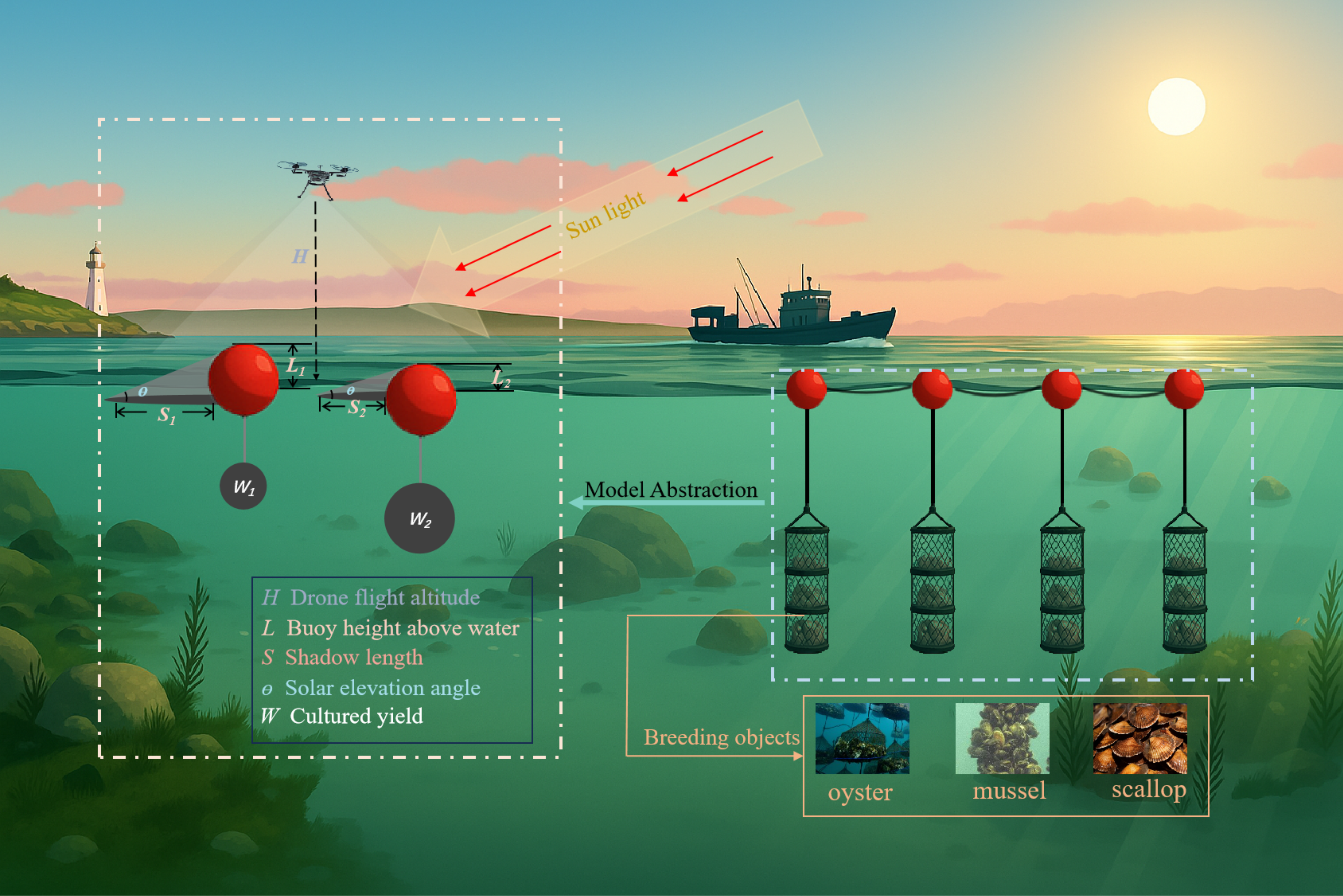
The yield estimation model uses the buoy as the central analytical unit in longline aquaculture systems. The balance between buoyancy and load establishes a stable physical relationship, which serves as the theoretical foundation for quantifying aquaculture yield. In suspended aquaculture operations, each buoy maintains the vertical orientation of the main ropes and functions as a mechanical indicator reflecting the total yield it supports. The mechanical equilibrium of the buoy-supported longline system is governed by the interaction between the upward buoyant force and the total downward force. The downward force is generated by the weight of the buoy and the attached culture units. As the yield increases during the growth process, the additional load leads to a deeper submersion of the buoy, thereby altering its visible geometry at the water surface and quantitatively linking the submersion depth to aquaculture yield. The geometric variation in the buoy represents a direct and observable manifestation of yield accumulation, providing a measurable remote-sensing signal that bridges physical equilibrium and production growth. When the buoy–rope system reaches equilibrium, the buoy can be regarded as being in static balance, forming a physically stable relationship between submersion depth and supported load that underpins the yield estimation model. The degree of buoy submersion provides an indirect but physically consistent indicator of the yield of suspended culture units and can be assessed without direct measurement. Because the submersion depth cannot be directly observed from UAV imagery, the estimation is achieved through the geometric projection of the shadow of the buoy. Under solar illumination, the shadow length varies systematically with the solar elevation angle, offering a measurable proxy for submersion depth. The integration of shadow geometry with solar position parameters enables quantitative reconstruction of the physical state of the buoy, allowing aquaculture yield to be estimated remotely with high precision and scalability across large farming areas. SGIA integrates the physical relationship between buoyancy and load with buoy shadow information from remote sensing imagery, combining the relationship between solar elevation angle and buoy geometry to provide a non-contact, scalable method for aquaculture yield assessment, as shown in Figure 1.

Figure 1. Conceptual illustration of UAV remote sensing-based yield estimation in longline aquaculture systems.

The yield of the cultured units can be determined based on the principle of Archimedes, which relates the buoyant force to the volume of water displaced by the submerged portion of the buoy. For a float of radius (R) and submersion depth (L), the displaced volume is given by the spherical cap geometry. Combining these relationships yields the buoyancy-based load model:

$$W_{\mathrm{l}\mathrm{o}\mathrm{a}\mathrm{d}}=\rho \cdot V_{\mathrm{d}\mathrm{i}\mathrm{s}\mathrm{p}\mathrm{l}\mathrm{a}\mathrm{c}\mathrm{e}\mathrm{d}}-W_{\mathrm{b}\mathrm{u}\mathrm{o}\mathrm{y}}$$

(1)

$$V_{\mathrm{d}\mathrm{i}\mathrm{s}\mathrm{p}\mathrm{l}\mathrm{a}\mathrm{c}\mathrm{e}\mathrm{d}}={\displaystyle \frac{\pi L^2(3R-L)}{3}}$$

(2)

$$W_{\mathrm{l}\mathrm{o}\mathrm{a}\mathrm{d}}=\rho {\displaystyle \frac{\pi L^2(3R-L)}{3}}-W_{\mathrm{b}\mathrm{u}\mathrm{o}\mathrm{y}}$$

(3)

where W_load represents the estimated yield of the suspended bivalves (kg), ρ is the water density (kg/m³), V_displaced is the displaced water volume (m³), and W_buoy is the self-weight of the float (kg).

Since the submersion depth (L) cannot be directly obtained from UAV imagery, it is inferred from the shadow length (S) and solar elevation angle (θ) using geometric projection. The solar elevation angle is determined from the geographic latitude (ϕ), solar declination (δ), and hour angle (h) at the time of image capture:

$$sin\left(\theta \right)=sin\left(\varphi \right)\cdot sin\left(\delta \right)+cos\left(\varphi \right)\cdot cos\left(\delta \right)\cdot cos\left(h\right)$$

(4)

$$L=S\cdot tan\left(\theta \right)$$

(5)

By integrating the buoyancy model (Equations (1)–(3)) with the geometric inversion model (Equations (4) and (5)), the final analytical expression for yield estimation is obtained:

$$W_{\mathrm{load}}=\rho \cdot {\displaystyle \frac{\pi (S\cdot \mathrm{t}\mathrm{a}\mathrm{n}(\theta \left){)}^2\right[3R-(S\cdot \mathrm{t}\mathrm{a}\mathrm{n}(\theta \left)\right)]}{3}}-W_{\mathrm{buoy}}$$

(6)

The derived analytical expression provides a complete transformation from UAV-derived shadow measurements to yield estimation for suspended longline bivalve aquaculture, enabling a physically interpretable, non-contact, and scalable method for spatial yield assessment.

2.2. SAM-Based Automatic Segmentation of Buoy Shadows

High-precision extraction of buoy shadows from UAV imagery is a prerequisite for accurately estimating buoy submersion depth and, consequently, for achieving reliable yield inversion results. The challenge lies in effectively separating the buoy and its shadow from the surrounding water surface under diverse lighting and environmental conditions. To overcome this challenge, SAM, developed by Meta AI, is adopted as the core framework for automated buoy and shadow segmentation [30]. SAM is a vision foundation model built upon a Transformer architecture, featuring powerful generalization and zero-shot segmentation capabilities. Unlike traditional convolutional neural network (CNN)–based approaches that rely on large-scale manually annotated datasets, SAM can perform segmentation directly from prompt information without task-specific retraining. The ability is particularly valuable in aquaculture applications, where labeled datasets are scarce and manual annotation is costly and time-consuming. SAM’s prompt-based design enables flexible adaptation to different imagery conditions, making the model well-suited for diverse aquaculture monitoring scenarios.

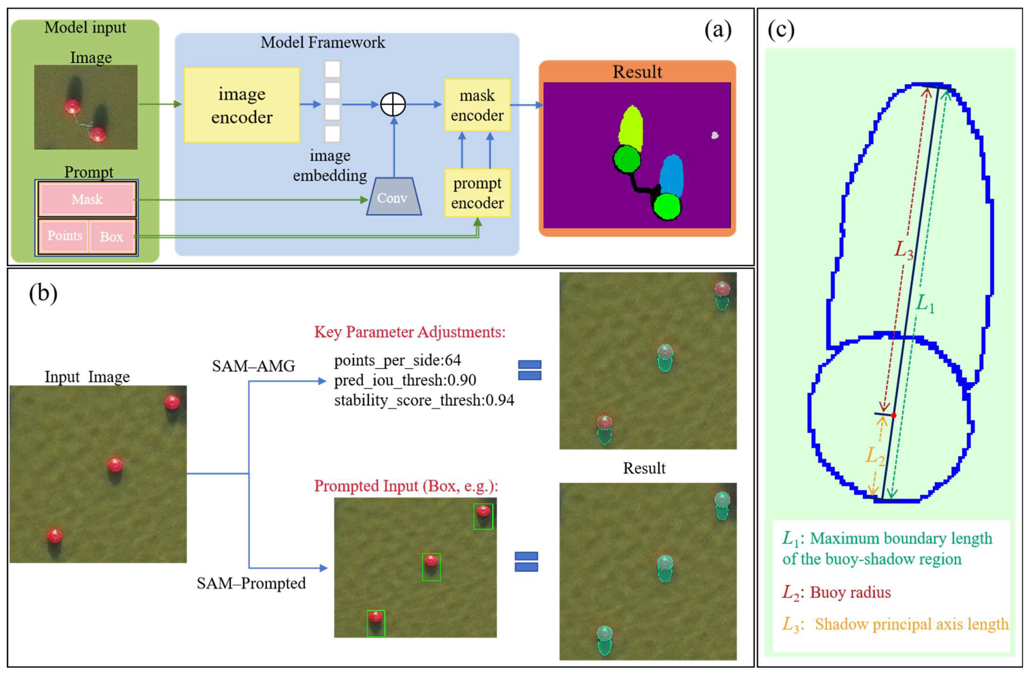
As illustrated in Figure 2, the SAM architecture consists of three primary components: the Image Encoder, Prompt Encoder, and Mask Decoder. The Image Encoder transforms the entire UAV image into high-dimensional feature embeddings, capturing both spatial and semantic information. The Prompt Encoder processes user-specified or automatically generated prompts—such as points, bounding boxes, or masks—while the Mask Decoder integrates the two feature streams to generate the final segmentation results.

Figure 2. Workflow of the Segment Anything Model (SAM) for buoy and shadow segmentation. (a) SAM architecture. (b) Example results of buoy shadow extraction. (c) Extracting Shadow Principal Axis Length.

SAM is primarily operated in the Automatic Mask Generation (AMG) mode for large-scale batch extraction of buoys and their shadows. In typical longline aquaculture environments, the water surface surrounding the buoys is relatively homogeneous, with minimal background clutter, which allows AMG to efficiently isolate the buoy–shadow pairs. To enhance segmentation performance for small targets and faint boundary contrasts, several key hyperparameters have been optimized. Specifically, points_per_side is increased to 64 to improve sampling density, pred_iou_thresh is set to 0.90 to exclude low-confidence masks, and stability_score_thresh is adjusted to 0.94 to ensure boundary consistency and mask reliability, thereby substantially improving the delineation of fine shadow contours, especially under variable solar elevation angles. After the shadow region is extracted, the buoy and shadow boundaries are treated as a single connected region. In the direction of the solar azimuth, the maximum boundary length of this region is identified. The radius of the buoy is then subtracted from this length to obtain the principal axis length of the shadow, as illustrated in Figure 2c.

When sunlight intensity is low or the contrast between the shadow and the surrounding water is weak—such as under overcast conditions or during high solar altitude periods—the AMG mode occasionally fails to recognize shadow regions, leading to incomplete or missing boundaries. To mitigate this issue, Prompted Segmentation is employed as a supplementary approach. By providing simple user prompts (e.g., bounding boxes or key points around the buoy), the model performs localized segmentation restricted to the prompted region. Such manually provided prompts significantly improve segmentation quality under challenging illumination conditions, effectively reducing false negatives and preserving the measurable geometry of shadow features.

By integrating the automation of AMG mode with the flexibility of Prompted Segmentation, SAM enables robust and adaptive extraction of buoy–shadow features across a wide range of environmental scenarios. Its ability to perform high-quality segmentation without task-specific retraining substantially reduces annotation costs while maintaining reliable accuracy. The resulting segmentation masks provide essential geometric information for the subsequent computation of shadow length and solar projection, ensuring that the derived inputs for yield inversion are both consistent and precise.

3. Experiments

3.1. Experimental Design

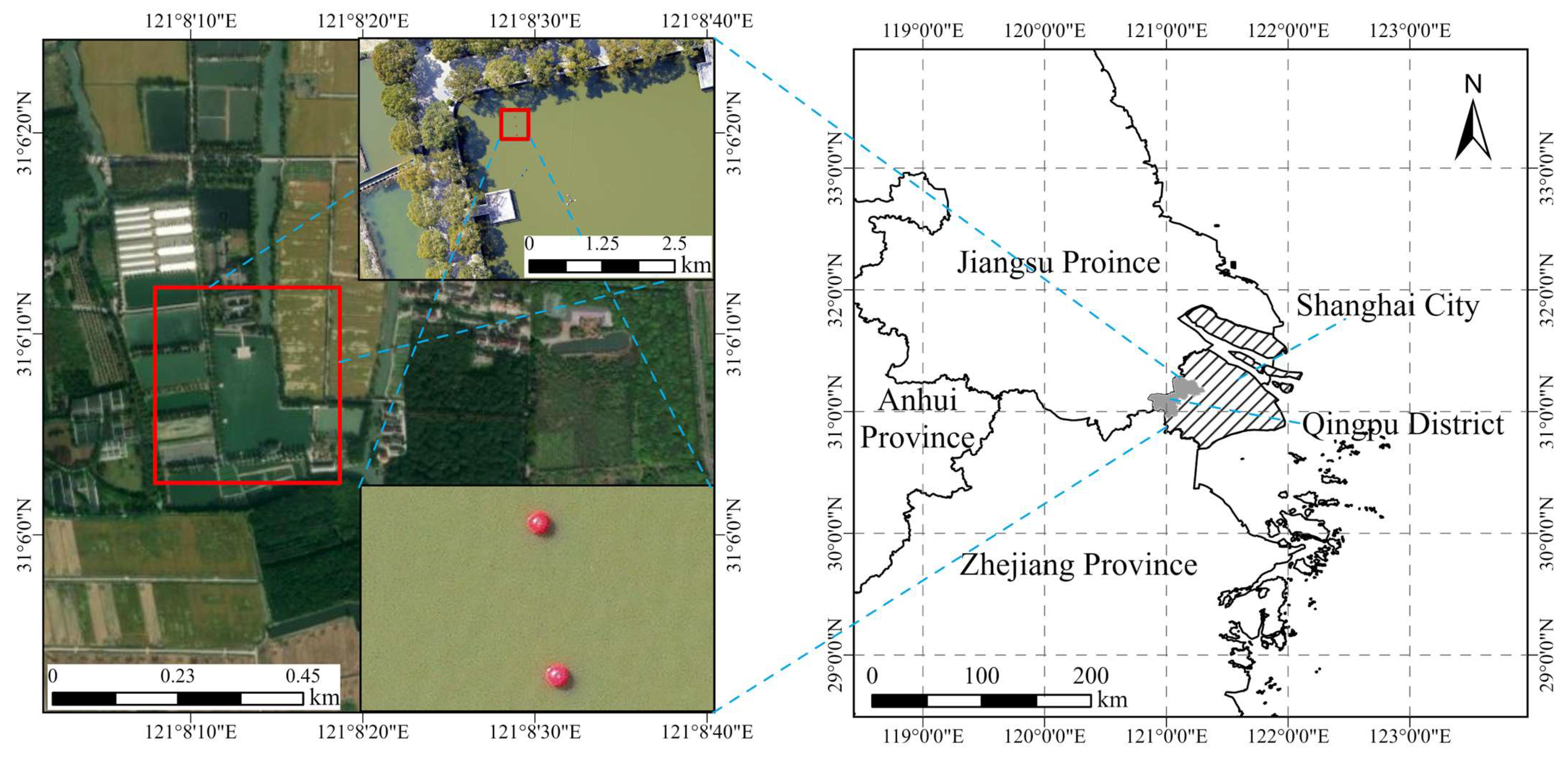
The controlled simulation experiment, conducted from March 18 to 19, 2025, in an enclosed freshwater pond in Qingpu District, Shanghai, China (31.10° N, 121.13° E), aimed to verify the feasibility and accuracy of the proposed UAV-based aquaculture yield estimation method grounded in shadow geometry analysis. The site provided a relatively stable aquatic environment with minimal wind disturbance, clear water, and uniform illumination, making it ideal for reconstructing simplified longline aquaculture structures under controlled conditions (Figure 3). The pond measured approximately 30 m in length, 15 m in width, and had an average water depth exceeding 2 m near the banks, meeting the requirements for buoy submersion and shadow projection observation during UAV imaging.

Figure 3. Experimental area in Qingpu District, Shanghai.

Three sets of buoy systems were designed to simulate varying loading conditions representative of longline aquaculture units. Each system consisted of a standard polyethylene spherical buoy with a diameter of approximately 0.3 m. The diameter of the buoys was measured using a ruler, with an accuracy of ±1 cm. The self-weight of each buoy was approximately 1.9 kg, measured using an electronic scale, with a measurement precision of ±100 g. At the lower end of each rope, weights of varying magnitudes were attached to replicate the increasing biomass loads encountered during different stages of culture growth. This configuration produced three distinct buoy submersion states, leading to corresponding variations in the length and geometry of their projected shadows on the water surface, which collectively provided the empirical foundation for establishing a quantitative relationship between buoy shadow characteristics and yield.

The experimental design involved UAV flights conducted under varying solar elevation angles. The UAV missions were carried out on two days: 17 March and 18 March 2025. On 17 March, flights were conducted at 15:35 and 16:30, with flight altitudes ranging from 80 to 130 m, capturing a total of 5 images in each batch. On 18 March, the flights were carried out at 16:15 and 16:21, with flight altitudes also ranging from 60 to 130 m, capturing 7 images for each batch. The flight altitude varied from 60 m to 120 m, corresponding to a ground sampling distance (GSD) of approximately 0.8–1.5 cm/pixel, ensuring sufficient spatial resolution for accurate identification of buoys and their shadows. The UAV used was the DJI Matrice 300 (M300), manufactured by DJI Innovations, headquartered in Shenzhen, China, with a maximum flight time of up to 50 min, making it suitable for the small-scale survey flights conducted during the study. The total area covered by the UAV during the missions was approximately 1.5 square kilometers, with the stability of the UAV flight performance ensuring consistent data capture across varying solar elevation angles.

Although eleven flight missions were completed in total, only four batches corresponding to the lowest solar elevation angles (approximately 10–30°) were selected for data analysis. The low-angle conditions provided the clearest and most stable shadow geometry, thereby minimizing measurement uncertainty and enhancing the reliability of geometric inversion and yield estimation. All acquired images were timestamped and georeferenced, with detailed metadata recorded to support subsequent solar position calculations and shadow-based geometric modeling.

3.2. Experimental Equipment

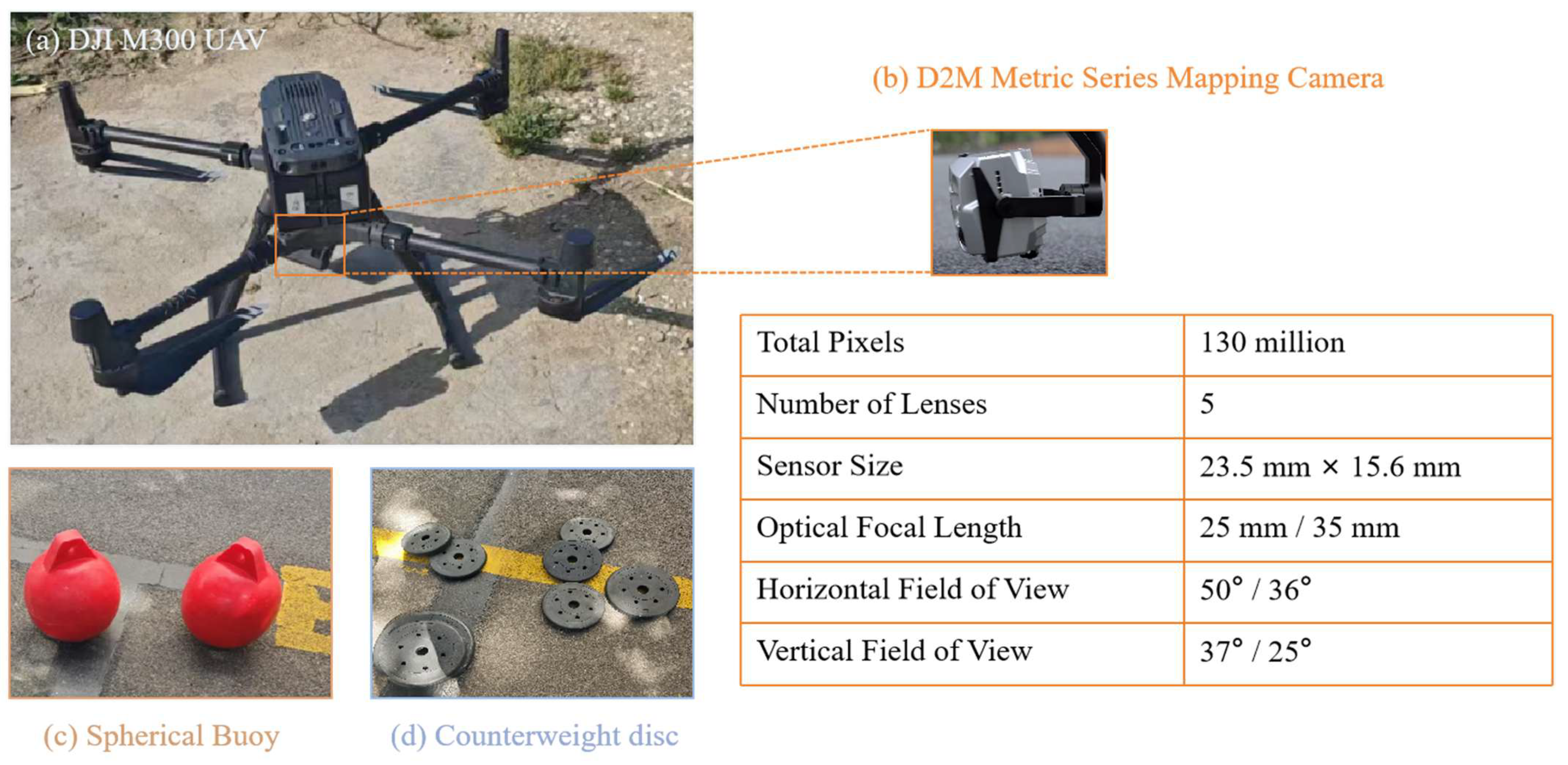
A DJI Matrice 300 (M300) multi-rotor UAV was used as the aerial imaging platform (Figure 4a). The M300 was a professional industrial-grade UAV characterized by excellent flight stability, strong payload capacity, and precise autonomous navigation performance, making it well-suited for high-resolution data acquisition tasks in complex environmental conditions. The UAV provided centimeter-level positioning accuracy through its built-in Real-Time Kinematic (RTK) system, which ensured consistent flight trajectories and minimized spatial distortion in the captured imagery. The stable operation and precise waypoint control of the M300 made it particularly suitable for repeated small-scale surveys requiring geometric consistency.

Figure 4. Experimental equipment.

The UAV was equipped with a D2M series photogrammetric camera (Figure 4b), featuring a 1.3-billion-pixel CMOS sensor and a 25 mm or 35 mm fixed-focus lens. This camera is capable of capturing high-quality RGB imagery with sub-centimeter ground resolution. This combination of the M300 platform and the D2M camera formed a highly stable remote sensing system integrating both multi-angle observation and geometric precision, meeting the requirements for accurate shadow delineation and buoy geometry reconstruction. The high radiometric fidelity and sharp optical performance of the camera ensured clear visualization of buoy boundaries and shadow contours, which were essential for the segmentation and geometric inversion modeling stages.

3.3. Experimental Validation

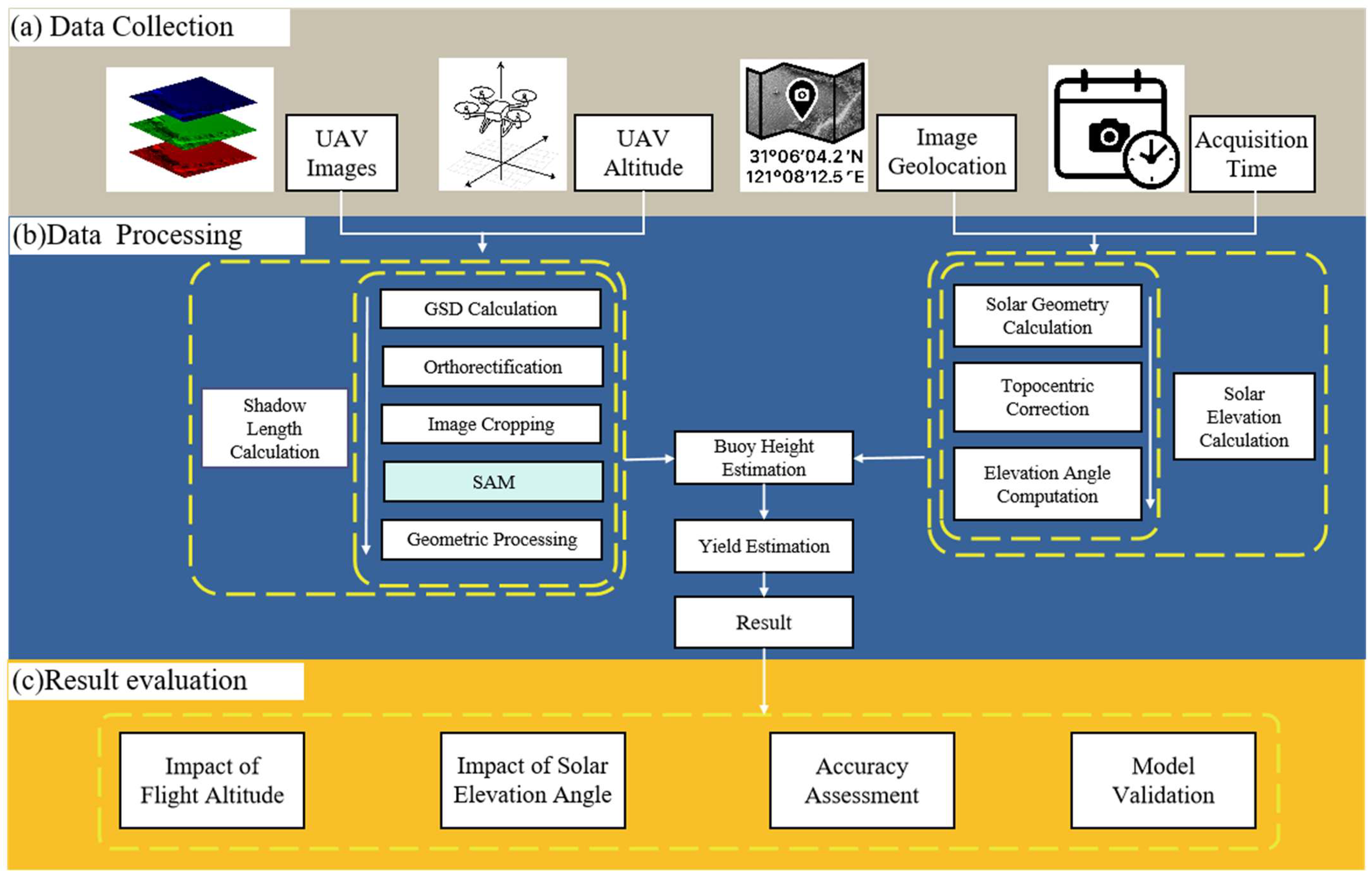
As illustrated in Figure 5, the validation workflow consisted of three main stages. In the data collection stage, a DJI Matrice 300 (M300) UAV equipped with a D2M photogrammetric camera was employed to capture high-resolution aerial imagery of the experimental area. The UAV recorded flight altitude, geographic coordinates, and acquisition time simultaneously during each mission. The flight altitudes ranged from 60 m to 120 m, resulting in a GSD of approximately 1.0–1.5 cm/pixel, ensuring the clear visibility of buoys and their shadows. The metadata, including timestamp, latitude, and longitude, served as critical input for subsequent solar geometry calculations and image georeferencing.

Figure 5. Workflow of the UAV-based yield estimation experiment.

In the data processing stage, all UAV images were first orthorectified and geometrically corrected to ensure spatial accuracy. SAM was then applied to automatically segment buoys and their shadows from the orthophotos, and the shadow principal axis length was extracted as the key geometric parameter for inversion. The solar elevation angle was calculated using the acquisition time and geographic coordinates recorded by the UAV. These parameters—shadow length, solar elevation angle, and buoy geometry—were integrated into the inversion model established in Section 2.1 to estimate the buoy submersion depth and yield. The estimation results from all batches were archived for subsequent accuracy evaluation and comparative analysis.

In the result evaluation stage, model performance was analyzed from two perspectives: (i) the influence of flight altitude and solar elevation angle on inversion accuracy, and (ii) quantitative validation of the estimated yield against reference measurements. Four statistical indicators—Root Mean Square Error (RMSE), Mean Absolute Error (MAE), Mean Absolute Percentage Error (MAPE), and the coefficient of determination (R²)—were used to comprehensively assess model accuracy, relative deviation, and overall fitting performance. This end-to-end workflow established a complete and traceable validation process from UAV image acquisition to inversion accuracy assessment, confirming that the proposed approach enabled high-precision, stable, and reproducible yield estimation in controlled aquaculture environments.

A systematic comparative validation experiment was conducted to verify the accuracy and robustness of the proposed yield estimation model based on buoy shadow length inversion under actual remote sensing image conditions. The objective of the experiment was to evaluate the estimation accuracy of the model for buoy submersion depth and the corresponding yield under varying load conditions, lighting periods, and flight altitudes. A DJI M300 UAV equipped with a high-resolution photogrammetric camera was used to perform aerial imaging tasks, with flights conducted in the morning, at noon, and in the afternoon, corresponding to different solar altitude angles. This setup aimed to examine the impact of imaging time on shadow projection geometry and estimation performance. Flight altitudes were set between 60 and 120 m, ensuring a spatial resolution better than 1.5 cm/pixel, thereby guaranteeing high-quality shadow feature visibility in the images.

The acquired UAV images were processed using SAM to automatically segment the buoys and their shadows, extracting the length of the principal axis of the shadow. The solar altitude angle was calculated by combining the image capture time and geographic location. Subsequently, the buoy submersion depth and yield were inferred based on the geometric model described in Section 2.1.

4. Result

4.1. Experimental Results

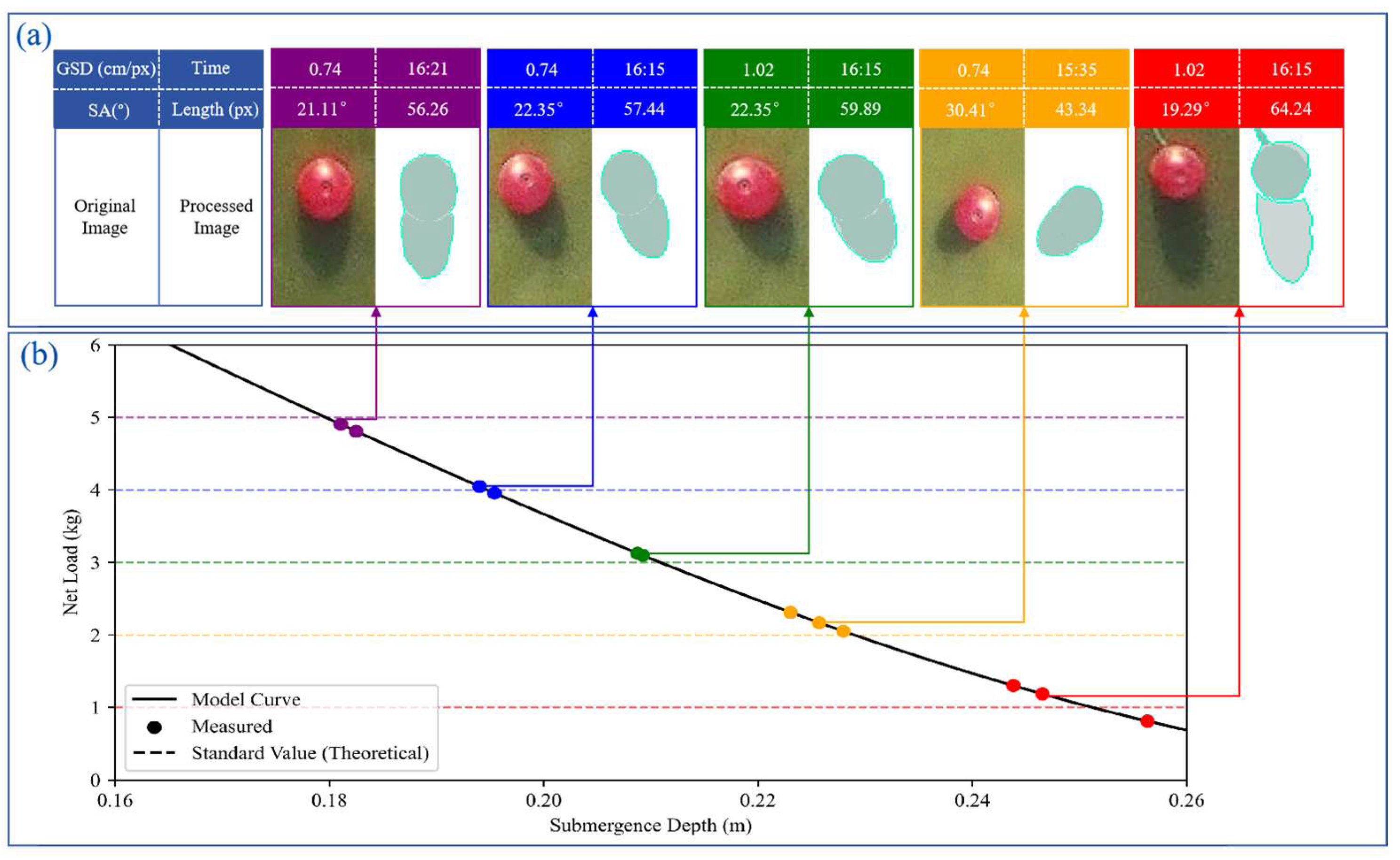
The physical foundation of the proposed UAV-based geometric inversion model, SGIA validated by the experimental results, with strong and consistent correlation between buoy submersion depth and aquaculture yield. As shown in Figure 6, the buoy submersion depth was derived from shadow length measurements obtained under multiple solar elevation angles, while the corresponding net load values were determined from the applied test weights. As shown in Figure 6a, representative examples of buoy and shadow segmentation results generated by SAM under different solar illumination conditions are presented. Each case corresponds to a specific imaging time and solar elevation angle (ranging from 19.29° to 30.41°) and was captured at flight altitudes with GSD between 0.74 and 1.02 cm/pixel. The segmentation results show that SAM successfully delineated both buoy boundaries and shadow contours with high precision, even under variable illumination and reflection conditions. Minor differences in shadow length among the samples reflect the influence of both buoy submersion depth and solar elevation on the projected shadow geometry. Figure 6b presents the quantitative comparison between theoretical values and model-estimated results. The predicted net load (black solid curve) exhibited a strong monotonic decreasing trend with increasing submersion depth, consistent with the theoretical expectation that higher loads lead to deeper buoy immersion. The experimental measurements (red dots) closely followed the model curve, with an R² of 0.985 and a mean absolute percentage error (MAPE) of 9.19%. These results indicate that the proposed model accurately captured the physical relationship between buoy geometry and yield, validating its reliability and predictive stability.

Figure 6. Examples of buoy imagery, automatic segmentation results, and comparison between submergence depth and net load for different weight classes. (a) Buoy images with segmentation results; (b) Comparison of submergence depth and net load.

Furthermore, comparison across different loading states and solar elevation angles revealed that the model achieved the highest accuracy under moderate solar angles (20–25°), where shadow features were most distinct. However, a slightly larger deviation was observed under the 1 kg load condition, which exhibited the highest relative error among all test cases. This deviation was primarily attributed to the extremely low submersion and light mass of the buoy, making it more susceptible to wind-induced lateral displacement on the water surface. The resulting horizontal movement caused minor distortions in the captured shadow geometry and introduced measurable errors in length estimation. Despite this, the overall fitting performance remained stable across all loading conditions, demonstrating the robustness and reliability of the proposed model.

4.2. Field Application

The field application was conducted in Fuding, a major oyster-farming region located at the junction of the East China Sea and northern Fujian Province. Fuding’s coastal zone features extensive tidal flats, high water transparency, and stable hydrodynamic conditions, together forming an ideal environment for suspended bivalve cultivation. Longline oyster farming dominates local aquaculture activities, producing continuous arrays of buoys and ropes that extend several kilometers offshore. According to local reports, the total oyster farming area in Fuding covers approximately 10,000 mu (about 670 hectares), with an annual output of around 45,000 tons. At the provincial scale, Fujian Province maintains over 37,000 hectares of oyster-farming area and an annual production exceeding 2 million tons. The cultivation structures in Fuding are arranged in dense linear grids, where polyethylene buoys serve simultaneously as flotation devices and load-bearing indicators of aquaculture yield. Such a high-density configuration, combined with variable water color, tidal currents, and surface reflection, presents major challenges for conventional remote-sensing and image-segmentation approaches. Therefore, the Fuding aquaculture zone serves as a representative and demanding testbed for assessing the robustness and scalability of the buoy–shadow–based inversion model under real-world operational conditions.

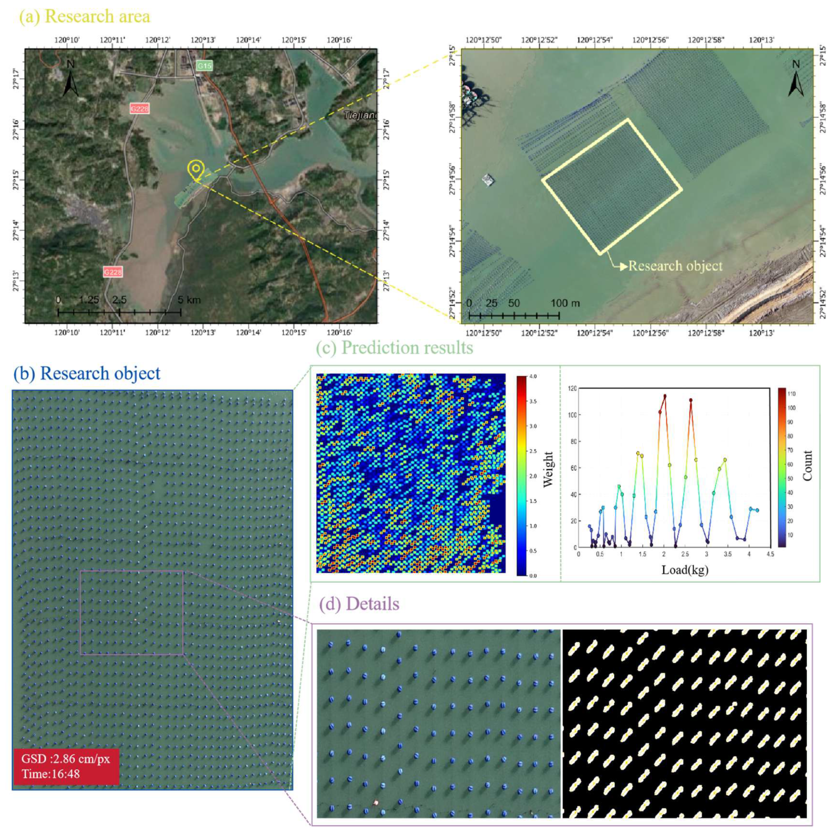
A large-scale field experiment was conducted in the Fuding oyster aquaculture area (Figure 7a) to assess the applicability of the proposed UAV-based yield estimation framework. UAV imagery was captured at a flight altitude of 200 m, yielding a ground sampling distance (GSD) of 2.86 cm/pixel. Compared with low-altitude imaging, the higher altitude resulted in reduced spatial resolution, leading to slightly blurred buoy–shadow boundaries and introducing uncertainty in the accurate extraction of shadow length. This decrease in geometric clarity inevitably caused a minor reduction in the estimation accuracy of the inversion model.

Figure 7. Field application of the proposed UAV-based yield estimation method in the Fuding aquaculture area.

Despite these limitations, the SAM-based segmentation framework demonstrated stable and adaptive performance across the complex large-scale aquaculture scene (Figure 7b). Approximately 1180 buoy shadows were successfully detected and retained for further analysis. Based on the established geometric inversion model, the draft depth and corresponding load of each buoy were calculated. The resulting spatial yield map (Figure 7c) revealed pronounced heterogeneity in load distribution: most buoys exhibited net loads between 2.0 and 4.5 kg, with a clear frequency peak near 3.5 kg, consistent with the expected biomass level at this cultivation stage. Detailed visualization of local subregions confirmed that SAM effectively delineated individual buoys and their corresponding shadows even in densely packed farming grids. Nevertheless, occasional segmentation errors occurred in zones with short shadows, high surface reflectance, or overlapping structures, which occasionally led to minor overestimation or underestimation of load values. Overall, the field experiment verified that the proposed yield estimation approach can be successfully extended from controlled laboratory conditions to real operational aquaculture environments. Although higher flight altitudes reduce fine-scale precision, the method still captures the essential spatial patterns of yield distribution with reasonable accuracy. These results underscore the practicality and scalability of UAV-based buoy shadow geometry analysis for precision monitoring and quantitative assessment in marine longline farming systems, offering a reliable technical tool for aquaculture production management and environmental supervision.

5. Discussion

5.1. Performance Evaluation of SAM for Buoy Shadow Segmentation

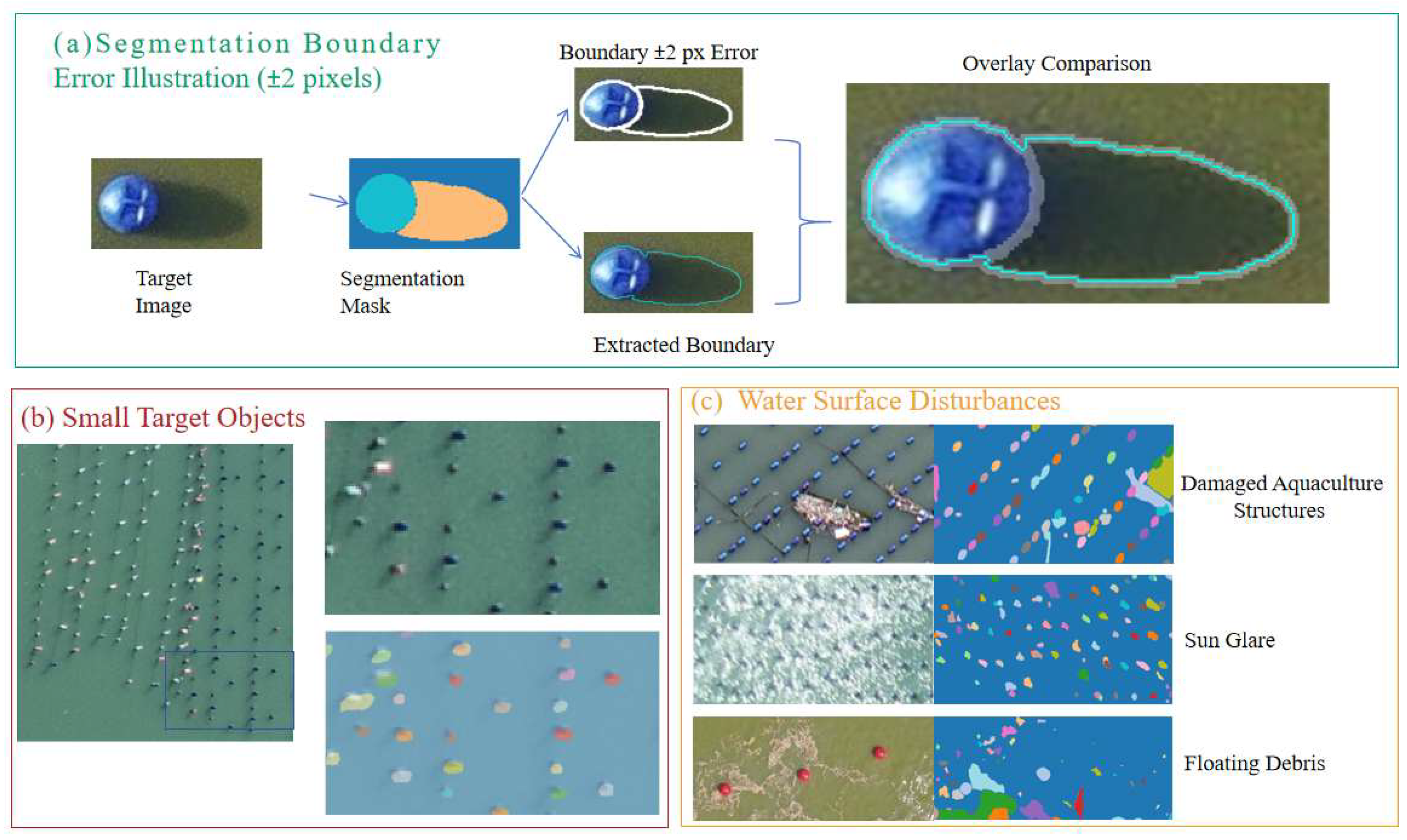
Accurate buoy shadow segmentation is essential for reliable geometric inversion of aquaculture yield based on UAV imagery, as boundary precision directly affects the measurement of shadow length and the stability of model inversion. Because the actual shadow length of floating buoys cannot be directly measured over water, no absolute ground-truth reference was available for quantitative validation of segmentation accuracy. Although the Segment Anything Model (SAM) demonstrates strong generalization ability, its performance over dynamic water surfaces is inevitably affected by wave motion, ripples, and specular reflections, which blur or distort the true shadow boundary. Empirical inspection of multiple UAV image samples revealed that SAM’s segmentation results consistently enclosed the actual shadow extent within a narrow margin of approximately ±2 pixels, effectively accommodating minor boundary fluctuations while maintaining geometric integrity. Therefore, a boundary tolerance of ±2 pixels was defined as the accuracy criterion for SAM segmentation (Figure 8a), ensuring reliable shadow extraction for subsequent inversion modeling.

Figure 8. Segmentation boundary error definition and performance evaluation.

Although SAM demonstrated strong overall performance, several conditions were identified in which segmentation reliability was reduced. Small target objects (Figure 8b) posed a notable challenge: when buoys occupied only a limited number of pixels in wide-area surveys, their spatial representation became insufficient for SAM to generate stable masks. This often led to incomplete segmentation, fragmented boundaries, or even complete omission of targets—issues that were particularly evident when UAVs operated at higher altitudes, where resolution decreased and pixel footprints shrank. Water-surface disturbances further introduced additional sources of error (Figure 8c). Floating debris, damaged aquaculture structures, and foam patterns on the water could mimic the appearance of buoy shadows in both geometry and spectral contrast. These elements often confused the model, resulting in false positives or erroneous boundary extensions; for example, fragments of broken ropes or cages were sometimes misidentified as elongated shadow features, undermining the accuracy of shadow-length measurements. Sun glare and specular reflection also complicated shadow extraction—under strong illumination, high-intensity glints sometimes overlapped or masked the true shadow regions. SAM occasionally misclassified glare patches as background, leading to incomplete segmentation, or confused bright-glare boundaries with shadow edges, creating inconsistent masks. The impact of sun glare was particularly pronounced when the solar altitude was high, coinciding with shorter shadows that were already difficult to delineate.

The experimental analysis emphasized that while SAM had provided robust zero-shot segmentation in relatively clean and well-illuminated scenarios, its accuracy degraded in environments characterized by very small target objects, cluttered backgrounds, or severe optical interference. These findings suggest that SAM’s zero-shot segmentation, though powerful, remains sensitive to variations in target scale and lighting complexity. Improving segmentation reliability therefore requires the integration of preprocessing strategies (e.g., glare suppression, background filtering), the adoption of multi-view UAV imaging to enhance feature consistency, or the combination of SAM with prompt-based refinement for more controlled segmentation. Such measures can further enhance the robustness and adaptability of buoy-shadow extraction in real-world aquaculture environments.

5.2. Influence of Solar Altitude Angle on Model Accuracy

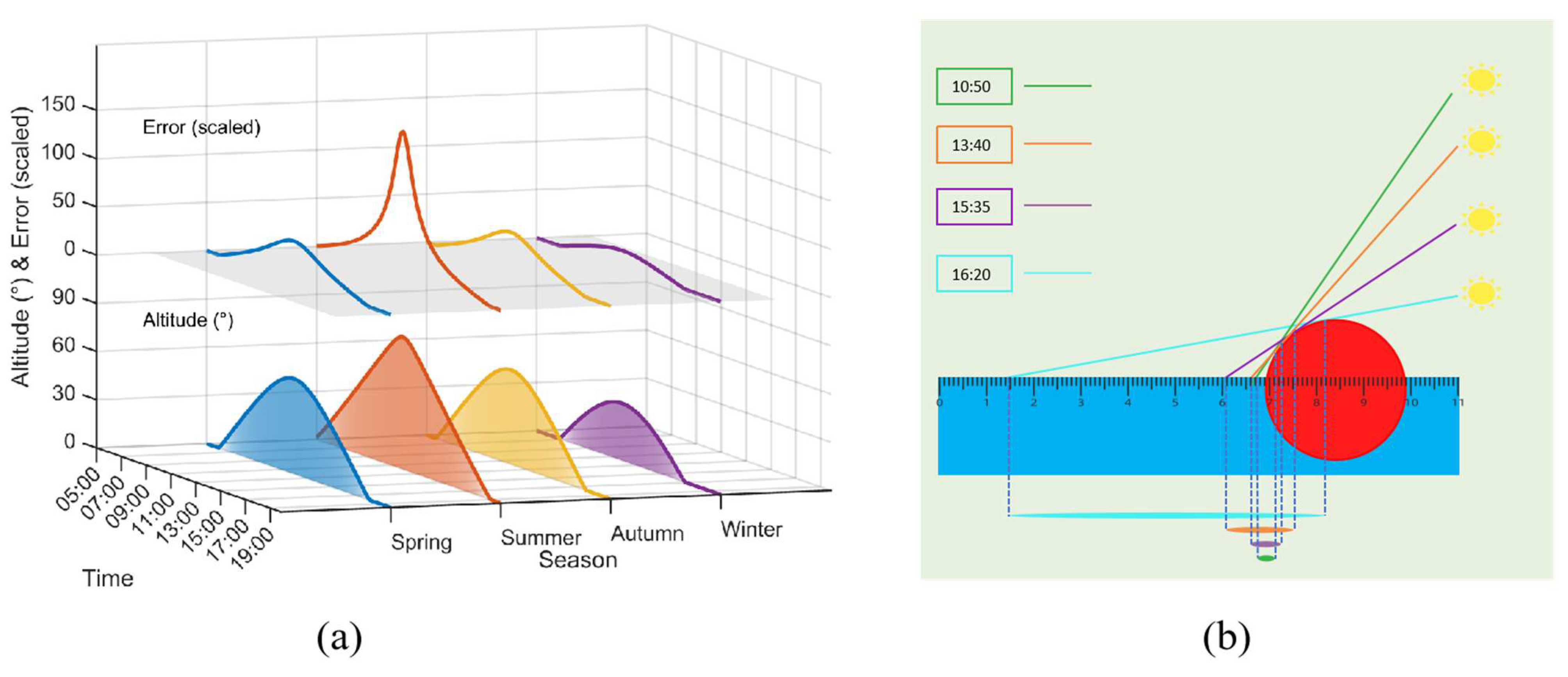
Solar altitude angle plays a crucial role in UAV-based geometric inversion for aquaculture yield estimation, as it determines illumination geometry, governs the temporal distribution of UAV observation periods, and directly influences model accuracy (Figure 9a). Under low solar-altitude conditions, the duration of effective observations varied markedly among seasons. In winter, the overall solar altitude remained low, and illumination periods below 30° lasted for more than six hours, providing the broadest time window for shadow-based observations. In spring and autumn, the solar altitude changed more gradually, and low-angle conditions lasted for about two hours, typically occurring around 8:00 a.m. and 4:00 p.m. In summer, the sun rose earlier and ascended rapidly; illumination with solar altitude angles below 30° persisted for only about one hour, mainly before 7:00 a.m. and shortly before sunset, resulting in a very limited observation period. Estimation errors increased significantly under high solar-altitude conditions. When the solar altitude exceeded 70°, buoy shadows became extremely short and overlapped with buoy edges, while strong specular reflections reduced image contrast, making it difficult for the SAM model to accurately detect the start and end positions of shadows. Because the geometric inversion equation contained trigonometric functions of the solar altitude angle, its derivative became highly sensitive as the angle approached the vertical direction, thereby amplifying small measurement deviations in shadow length. For example, as the solar altitude increased from 45° to 80°, the same one-pixel measurement bias caused the inversion error to more than double. Extremely low solar-altitude angles also reduced observation accuracy. When the solar altitude fell below approximately 10–25°, solar irradiance decreased sharply, overall image brightness declined, and surface-scattered light intensified, resulting in blurred shadow boundaries that hindered accurate extraction by the SAM model. Both excessively high and low solar altitude angles reduce the stability of shadow recognition and inversion. The optimal observation window occurs when the solar altitude ranges between 10° and 25°, during which shadows are of moderate length, boundaries remain distinct, and the model achieves the highest accuracy.

Figure 9. Influence of solar altitude angle on geometric inversion accuracy. (a) Variation of solar altitude and model error across seasons. (b) Change in the sunlight tangent point on the buoy under different solar altitude angles.

The solar altitude angle also introduced systematic bias by altering the geometric tangent point between sunlight and the buoy surface (Figure 9b). Taking a spherical buoy as an example, at low solar altitude angles, the influence of the geometric tangent point between sunlight and the buoy surface on the model can be neglected due to the diffraction effect of light. In this case, the diffraction effect of light smooths the formation of the shadow, and the offset of the shadow’s starting point is small, so the variation in the geometric tangent point has a minimal impact on the model. As the solar altitude increases, the sunlight tangent point moves downward along the buoy surface, causing the starting point of the shadow to shift inward, ultimately leading to a shorter shadow length. Specifically, as the solar altitude increases, the sunlight tangent point moves upward along the buoy surface, causing the starting point of the shadow to shift outward. For example, at 10:50 a.m., when the solar altitude is about 50°, the shadow originates nearly at the boundary of the buoy. By 1:40 p.m., when the solar altitude drops to about 45°, the starting point shifts outward by approximately 0.5 times the buoy radius. At 3:35 p.m., when the solar altitude decreases to about 30°, the offset reduces to about 0.2 times the radius. By 4:20 p.m., when the solar altitude is about 25°, the tangent point approaches the center of the buoy, and the shadow nearly returns to its theoretical position.

In the future, to overcome the current limitation of the method within the solar altitude angle range of 10° to 25°, a geometric approach can be adopted by treating the buoy as a sphere and using trigonometric functions to accurately calculate the tangent point between the sunlight and the buoy surface. Specifically, as the solar altitude changes, the tangent point between the sunlight and the buoy surface also shifts, affecting the formation of the shadow. By establishing a lighting model based on the spherical geometry of the buoy, the tangent point can be calculated using the solar incidence angle and the buoy radius, which will determine the starting point of the shadow.

5.3. Impact of Different Flight Altitudes on Experimental Accuracy

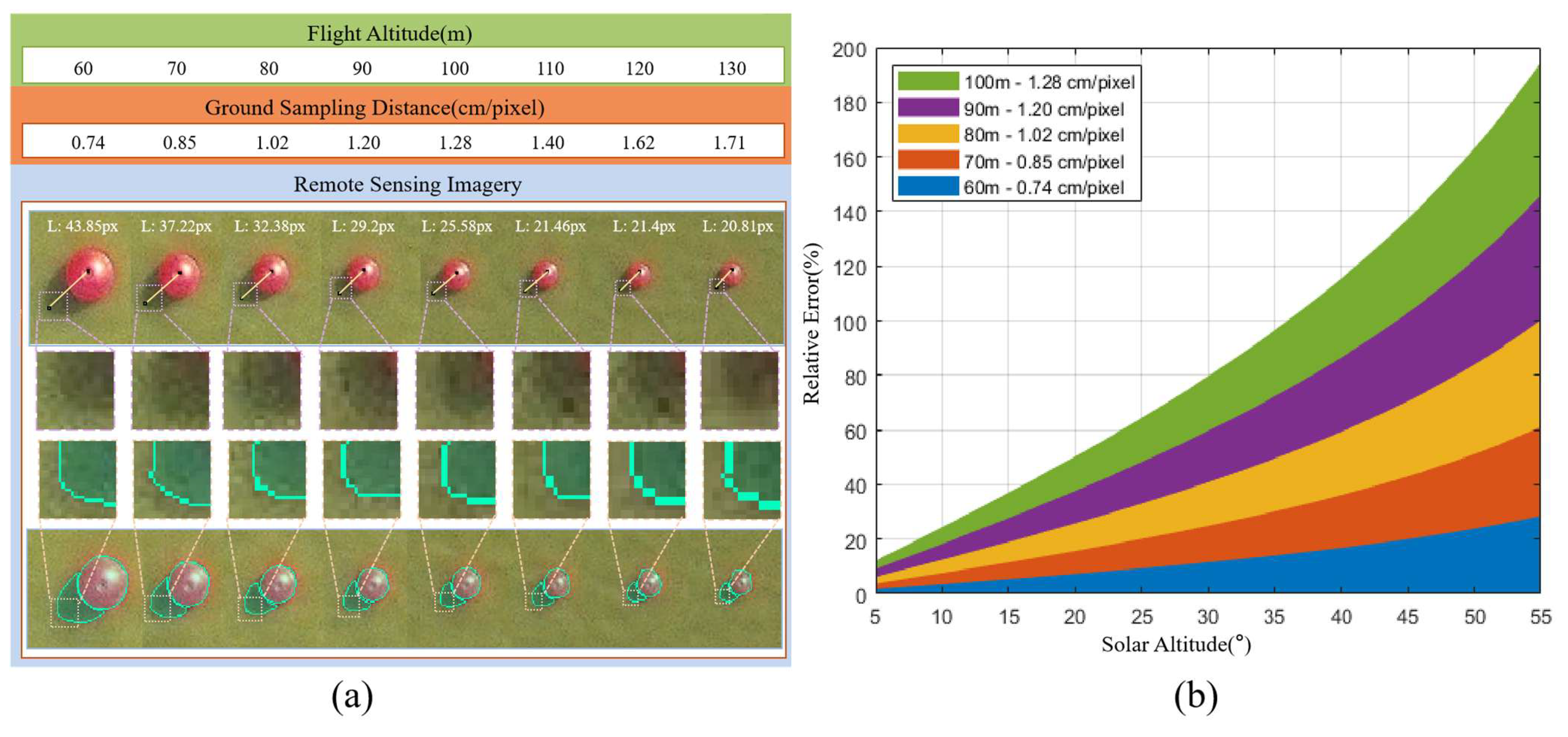
Flight altitude, as a critical factor in UAV-based geometric inversion for aquaculture yield estimation, determined image resolution and directly affected the accuracy of buoy–shadow feature extraction and model stability. As shown in Figure 10a, when the flight altitude increased from 60 m to 130 m, the GSD expanded from 0.74 cm/pixel to 1.71 cm/pixel, leading to a gradual decline in image clarity. At lower altitudes (60–80 m), the buoy and shadow contours remain sharp, and the shadow’s principal axis can be measured stably and accurately. In contrast, at higher altitudes (≥100 m), insufficient spatial sampling caused buoy and shadow structures to become increasingly blurred. Under these conditions, SAM had difficulty distinguishing shadow boundaries, leading to discontinuous edges, distorted shadow shapes, and unstable shadow-length measurements, all of which introduced significant errors into the inversion process.

Figure 10. Influence of flight altitude on inversion accuracy. (a) Variation in image clarity and shadow segmentation with different flight altitudes. (b) Relationship between relative error and solar altitude under various flight altitudes.

The quantitative relationship between relative error, flight altitude, and solar altitude was shown in Figure 10b. Across all solar altitude angles, higher flight altitudes consistently produced larger inversion errors, and this discrepancy became more pronounced under high solar altitude conditions. Short shadows at high solar angles were more susceptible to measurement uncertainty when image resolution was reduced, while the non-linear trigonometric nature of the inversion equation further amplified these small deviations. For instance, at a solar altitude of 40°, the relative error at 100 m exceeded that at 60 m by more than four times, illustrating the combined effects of reduced spatial resolution and increased geometric sensitivity at greater heights.

Low-altitude UAV flights (60–80 m) are preferable for aquaculture monitoring when high geometric precision is required, particularly from a practical standpoint. Maintaining a GSD finer than 1.0 cm/pixel ensures that buoy and shadow boundaries remain distinct and that SAM segmentation performs reliably. As shown in Figure 10b, when the flight altitude increases from 60 m to 130 m, the GSD expands from 0.74 cm/pixel to 1.71 cm/pixel, leading to a gradual decline in image clarity. The method remains stable at altitudes between 60 and 80 m, with a GSD range from 0.74 to 1.02 cm/pixel, which corresponds to the acceptable threshold for reliable buoy and shadow feature extraction. Although higher flight altitudes improve coverage efficiency, the associated degradation in spatial resolution substantially reduces the extractability of geometric features and increases inversion uncertainty. At altitudes above 100 m, the GSD increases beyond the acceptable threshold of 1.0 cm/pixel, significantly affecting the accuracy of shadow extraction and increasing uncertainty in the yield estimation process.

5.4. Impact of Environmental Factors on Model Accuracy

The impact of environmental factors on the model’s accuracy primarily lay in the effect of wind on water surface waves, which in turn influenced the position and movement of the buoy. In suspended longline aquaculture, most of the structure, including the buoy, was submerged underwater. Therefore, the direct impact of wind force on the buoy was relatively minimal. However, the effect of wind on the water surface, particularly the formation of waves, played a much larger role in the overall accuracy of the model. Wind-induced waves caused fluctuations in the position of the buoy, which led to errors in the geometric inversion calculations. According to data provided by the National Weather Service, we categorized the impact of wind on waves based on wind force levels and the resulting wave height into three categories: Calm, Mild Waves, and Active Waves (Table 1).

Table 1. Summary of selected UAV flight batches under the lowest solar elevation angles used for geometric inversion analysis.

Category	Wind Force Level	Wind Force Name	Wind Speed (knots)	Wind Force Impact on Water Surface	Wave Height (m)
Calm	0	Calm	0	Like a mirror	0
Mild Waves	1	Light air	1–3	Light ripples	0.1
Active Waves	2	Light breeze	4–6	Small waves	0.2–0.3
	3	Gentle breeze	7–10	Waves with breaking crests	0.6–1

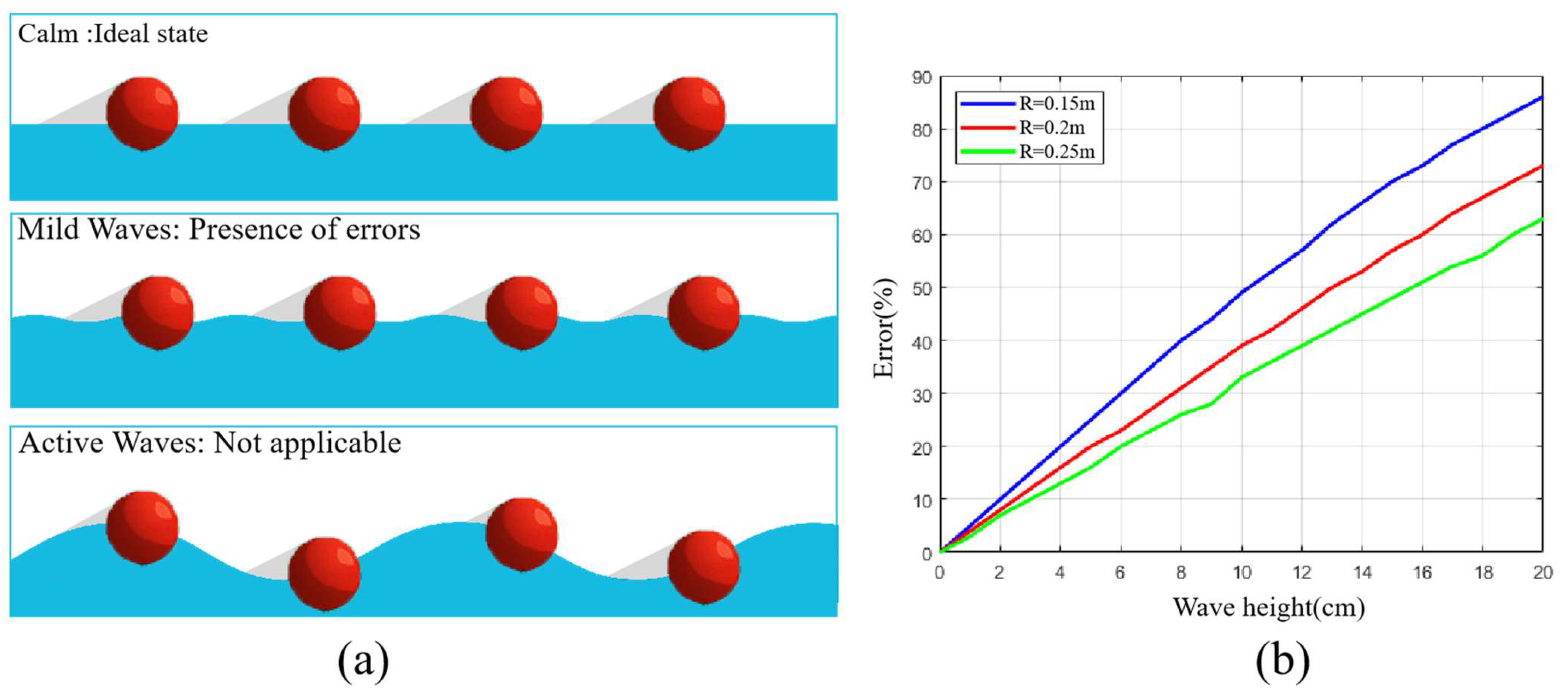
In contrast, under active sea conditions, where wind speeds exceeded 7 knots and wave heights reached up to 2 m, the SGIA method faced more significant challenges. The water surface became more turbulent, and the buoy experienced greater pitching and drifting, leading to a less stable shadow projection. Figure 11a illustrates the buoy’s behavior under three different wave conditions. In Calm conditions, the buoy was almost unaffected by the waves, remaining stationary and close to the ideal state. The shadow was stable and aligned with the buoy’s position, resulting in minimal model prediction errors. In contrast, under Mild Waves, the undulating waves began to affect the shadow, primarily along its longest axis. As the waves caused slight fluctuations in the buoy’s position, the shadow’s length and direction shifted, leading to increased prediction errors in the model. Nonetheless, the proposed method could still be somewhat applicable in this situation. Under Active Waves, the waves were larger, causing significant displacement in the buoy’s position, and the shadow was also notably impacted. Additionally, the waves may have generated white foam, which interfered with boundary extraction, making the model ineffective under such conditions and leading to large errors that were difficult to correct.

Figure 11. Buoy behavior and error analysis under different wave conditions. (a) Schematic of the buoy in Calm, Mild, and Active waves. (b) Error analysis under Mild waves for varying buoy radius and load at a solar altitude angle of 15°.

Figure 11b showed the relationship between peak height (in centimeters) and error for three different buoy radii (0.15 m, 0.2 m, and 0.25 m) under mild wave conditions at a solar altitude angle of 15°. As the peak height increased, the error for all three buoy radii also increased. When the peak height was less than 5 cm, the proposed method performed well, maintaining relatively low errors. Specifically, for the 0.15 m radius buoy (blue curve), the error was about 20% when the peak height was 5 cm; for the 0.2 m radius buoy (red curve), the error was close to 15% under the same conditions; and for the 0.25 m radius buoy (green curve), the error remained around 10%. This indicated that when the peak height was less than 5 cm, the model effectively minimized errors and performed well. As the peak height increased, the error gradually increased. At a peak height of 20 cm, the error for the 0.15 m radius buoy reached 80%, for the 0.2 m radius buoy, the error was about 70%, and for the 0.25 m radius buoy, the error was 60%. This phenomenon demonstrated that as the buoy radius increased, its resistance to wave-induced displacement improved, reducing the impact of wave-induced movement on the model’s error. Therefore, it is recommended that buoy yield estimation be conducted under calm water conditions. When the wave height exceeds 5 cm, the model becomes less effective for accurate yield estimation.

6. Conclusions

A Shadow Geometry Inversion for Aquaculture (SGIA) framework was developed for non-contact, direct yield estimation in suspended longline aquaculture using UAV imagery and buoy shadow geometry. By integrating solar altitude information, buoy physical parameters, and shadow length extracted through SAM, a physically interpretable inversion model was established to infer buoy load and culture biomass. Controlled experiments demonstrated strong consistency between predicted and measured loads (R² = 0.985, MAPE = 9.19%), confirming the stability and accuracy of the model in still-water environments. Field validation further verified that the method can capture the spatial variability of oyster yields, with load distributions matching the expected production levels during the mid-growth stage.

The method’s performance is highly dependent on the solar altitude angle and the water surface conditions, with optimal accuracy achieved when the solar altitude is between 10° and 25° and the wave height is below 5 cm. Additionally, flight altitude affects the method’s stability, with the optimal range for stable operation being 60–80 m, corresponding to a GSD finer than 1.0 cm/pixel. In these conditions, buoy and shadow boundaries remain distinct, ensuring reliable shadow extraction and yield estimation.

The SGIA method allows for automated, high-precision yield estimation without the need for physical sampling, making it a highly efficient tool for precision aquaculture management, particularly in longline aquaculture systems. By enabling spatially continuous yield monitoring, the SGIA framework supports better decision-making for farm management, enhances resource allocation, and helps optimize production. In addition, the ability to monitor yield variability in real-time—across vast longline farming areas—ensures that farmers can take immediate corrective actions, improving both the economic and ecological sustainability of aquaculture practices. Despite its limitations under complex optical conditions and dynamic water surfaces, SGIA offers a scalable, low-cost alternative to traditional manual sampling, significantly reducing labor costs and enhancing operational efficiency. The ability of the method to quickly and accurately assess longline aquaculture yields in real time makes it a powerful tool for enhancing the sustainability and profitability of aquaculture operations, particularly in large-scale and intensive farming systems. Nonetheless, limitations persist under complex optical conditions and dynamic water surfaces, where segmentation robustness and buoy motion may introduce uncertainty. Future work will focus on the following:

(1) Incorporating multi-source remote sensing data and deep learning refinement models to improve shadow segmentation and environmental adaptability;

(2) Developing a time-series monitoring framework for dynamic yield assessment across cultivation cycles;

(3) Integrating cloud computing and edge processing to facilitate real-time, intelligent implementation of UAV-based yield estimation in precision aquaculture.

References

1. Fong, C.R.; Gonzales, C.M.; Rennick, M.; Gardner, L.D.; Halpern, B.S.; Froehlich, H.E. Global Yield from Aquaculture Systems. Rev. Aquac. 2024, 16, 1021–1029. [Google Scholar] [CrossRef]
2. Taylor, D.; Saurel, C.; Nielsen, P.; Petersen, J.K. Production Characteristics and Optimization of Mitigation Mussel Culture. Front. Mar. Sci. 2019, 6, 698. [Google Scholar] [CrossRef]
3. Mascorda Cabre, L.; Hosegood, P.; Attrill, M.J.; Bridger, D.; Sheehan, E.V. Offshore Longline Mussel Farms: A Review of Oceanographic and Ecological Interactions to Inform Future Research Needs, Policy and Management. Rev. Aquac. 2021, 13, 1864–1887. [Google Scholar] [CrossRef]
4. Yildirim, Ş.; Erdem, Ö.A.; Sabanci, F.; Gökvardar, A.; Serdar, S.; Ertan, A. Effects of Different Culture Methods on Growth, Meat Yield, and Nutritional Composition of Mediterranean Mussels (Mytilus Galloprovincialis), South Side of Marmara Sea, Türkiye. Eur. Zool. J. 2024, 91, 869–889. [Google Scholar] [CrossRef]
5. Buck, B.H.; Ebeling, M.W.; Michler-Cieluch, T. Mussel Cultivation as a Co-Use in Offshore Wind Farms: Potential and Economic Feasibility. Aquac. Econ. Manag. 2010, 14, 255–281. [Google Scholar] [CrossRef]
6. Wang, X.; Xie, J.; Luo, Y.; Wang, X.; Guo, G.; You, X. Experimental Investigation of the Hydrodynamic Characteristics of Longline Aquaculture Facilities under Current and Wave Conditions. Fishes 2023, 8, 204. [Google Scholar] [CrossRef]
7. Heasman, K.G.; Scott, N.; Sclodnick, T.; Chambers, M.; Costa-Pierce, B.; Dewhurst, T.; Isbert, W.; Buck, B.H. Variations of Aquaculture Structures, Operations, and Maintenance with Increasing Ocean Energy. Front. Aquac. 2024, 3, 1444186. [Google Scholar] [CrossRef]
8. Ferriss, B.E.; Conway-Cranos, L.L.; Sanderson, B.L.; Hoberecht, L. Bivalve Aquaculture and Eelgrass: A Global Meta-Analysis. Aquaculture 2019, 498, 254–262. [Google Scholar] [CrossRef]
9. Stamp, T.; Pittman, S.J.; Holmes, L.A.; Rees, A.; Ciotti, B.J.; Thatcher, H.; Davies, P.; Hall, A.; Wells, G.; Olczak, A.; et al. Restorative Function of Offshore Longline Mussel Farms with Ecological Benefits for Commercial Crustacean Species. Sci. Total Environ. 2024, 951, 174987. [Google Scholar] [CrossRef]
10. Christensen, P.B.; Glud, R.N.; Dalsgaard, T.; Gillespie, P. Impacts of Longline Mussel Farming on Oxygen and Nitrogen Dynamics and Biological Communities of Coastal Sediments. Aquaculture 2003, 218, 567–588. [Google Scholar] [CrossRef]
11. Lacoste, E.; Drouin, A.; Weise, A.M.; Archambault, P.; McKindsey, C.W. Low Benthic Impact of an Offshore Mussel Farm in Îles-de-La-Madeleine, Eastern Canada. Aquac. Environ. Interact. 2018, 10, 473–485. [Google Scholar] [CrossRef]
12. Troell, M.; Joyce, A.; Chopin, T.; Neori, A.; Buschmann, A.H.; Fang, J.G. Ecological Engineering in Aquaculture—Potential for Integrated Multi-Trophic Aquaculture (IMTA) in Marine Offshore Systems. Aquaculture 2009, 297, 1–9. [Google Scholar] [CrossRef]
13. Rubino, R.; Lima, A.R.; Fox, J.M. Short-Term Effects of a Research-Scale Oyster Cage Aquaculture System on Sediment Transport, Water Quality, and Seagrass Meadow Health in Copano Bay, TX, USA. Front. Mar. Sci. 2024, 11, 1382153. [Google Scholar] [CrossRef]
14. Garcia, S.; Houle, K.; Suhrbier, A.; Hudson, B.; Ruesink, J. Estuarine Community Response to Longline Spacing in Intertidal Oyster Culture. Aquac. Environ. Interact. 2025, 17, 107–118. [Google Scholar] [CrossRef]
15. Rejeki, S.; Debrot, A.O.; Den Brink, A.M.; Ariyati, R.W.; Lakshmi Widowati, L. Increased Production of Green Mussels (Perna viridis) Using Longline Culture and an Economic Comparison with Stake Culture on the North Coast of Java, Indonesia. Aquac. Res. 2021, 52, 373–380. [Google Scholar] [CrossRef]
16. Román, A.; Prasyad, H.; Oiry, S.; Davies, B.F.R.; Brunier, G.; Barillé, L. Mapping Intertidal Oyster Farms Using Unmanned Aerial Vehicles (UAV) High-Resolution Multispectral Data. Estuar. Coast. Shelf Sci. 2023, 291, 108432. [Google Scholar] [CrossRef]
17. Román, A.; Tovar-Sánchez, A.; Olivé, I.; Navarro, G. Using a UAV-Mounted Multispectral Camera for the Monitoring of Marine Macrophytes. Front. Mar. Sci. 2021, 8, 722698. [Google Scholar] [CrossRef]
18. Wu, S.; Lu, Y.; Fan, W.; Zhang, S.; Wu, Z.; Wang, F. An Efficient Downwelling Light Sensor Data Correction Model for UAV Multi-Spectral Image DOM Generation. Drones 2025, 9, 491. [Google Scholar] [CrossRef]
19. Wu, S.; Nie, K.; Lu, X.; Fan, W.; Zhang, S.; Wang, F. A Solar Trajectory Model for Multi-Spectral Image Correction of DOM from Long-Endurance UAV in Clear Sky. Drones 2025, 9, 196. [Google Scholar] [CrossRef]
20. Ganie, P.A.; Khatei, A.; Posti, R.; Sidiq, M.J.; Pandey, P.K. Unmanned Aerial Vehicles in Fisheries and Aquaculture: A Comprehensive Overview. Environ. Monit. Assess. 2025, 197, 503. [Google Scholar] [CrossRef]
21. Liu, X.; Wang, Y.; Chen, T.; Gu, X.; Zhang, L.; Li, X.; Tang, R.; He, Y.; Chen, G.; Zhang, B. Monitoring Water Quality Parameters of Freshwater Aquaculture Ponds Using UAV-Based Multispectral Images. Ecol. Indic. 2024, 167, 112644. [Google Scholar] [CrossRef]
22. Rodofili, E.N.; Lecours, V.; LaRue, M. Remote Sensing Techniques for Automated Marine Mammals Detection: A Review of Methods and Current Challenges. PeerJ 2022, 10, e13540. [Google Scholar] [CrossRef] [PubMed]
23. Shamsolmoali, P.; Zareapoor, M.; Wang, R.; Zhou, H.; Yang, J. A Novel Deep Structure U-Net for Sea-Land Segmentation in Remote Sensing Images. IEEE J. Sel. Top. Appl. Earth Obs. Remote Sens. 2019, 12, 3219–3232. [Google Scholar] [CrossRef]
24. Machefer, M.; Lemarchand, F.; Bonnefond, V.; Hitchins, A.; Sidiropoulos, P. Mask R-CNN Refitting Strategy for Plant Counting and Sizing in UAV Imagery. Remote Sens. 2020, 12, 3015. [Google Scholar] [CrossRef]
25. Wang, J.; Fan, J.; Wang, J. MDOAU-Net: A Lightweight and Robust Deep Learning Model for SAR Image Segmentation in Aquaculture Raft Monitoring. IEEE Geosci. Remote Sens. Lett. 2022, 19, 4504505. [Google Scholar] [CrossRef]
26. Sui, B.; Jiang, T.; Zhang, Z.; Pan, X.; Liu, C. A Modeling Method for Automatic Extraction of Offshore Aquaculture Zones Based on Semantic Segmentation. ISPRS Int. J. Geo-Inf. 2020, 9, 145. [Google Scholar] [CrossRef]
27. Chen, H.-Y.; Cheng, S.-C.; Chang, C.-C. Semantic Scene Modeling for Aquaculture Management Using an Autonomous Drone. In Proceedings of the International Workshop on Advanced Imaging Technology (IWAIT), Yogyakarta, Indonesia, 5–7 January 2020; SPIE: Bellingham, WA, USA, 2020; Volume 11515, pp. 374–378. [Google Scholar]
28. Cheng, G.; Xie, X.; Han, J.; Guo, L.; Xia, G.-S. Remote Sensing Image Scene Classification Meets Deep Learning: Challenges, Methods, Benchmarks, and Opportunities. IEEE J. Sel. Top. Appl. Earth Obs. Remote Sens. 2020, 13, 3735–3756. [Google Scholar] [CrossRef]
29. Tuia, D.; Persello, C.; Bruzzone, L. Domain Adaptation for the Classification of Remote Sensing Data: An Overview of Recent Advances. IEEE Geosci. Remote Sens. Mag. 2016, 4, 41–57. [Google Scholar] [CrossRef]
30. Kirillov, A.; Mintun, E.; Ravi, N.; Mao, H.; Rolland, C.; Gustafson, L.; Xiao, T.; Whitehead, S.; Berg, A.C.; Lo, W.-Y.; et al. Segment Anything. In Proceedings of the IEEE/CVF International Conference on Computer Vision, Paris, France, 4–6 October 2023; pp. 4015–4026. [Google Scholar]
31. Osco, L.P.; Wu, Q.; De Lemos, E.L.; Gonçalves, W.N.; Ramos, A.P.; Li, J.; Junior, J.M. The Segment Anything Model (SAM) for Remote Sensing Applications: From Zero to One Shot. Int. J. Appl. Earth Obs. Geoinf. 2023, 124, 103540. [Google Scholar] [CrossRef]
32. Ren, Y.; Yang, X.; Wang, Z.; Yu, G.; Liu, Y.; Liu, X.; Meng, D.; Zhang, Q.; Yu, G. Segment Anything Model (SAM) Assisted Remote Sensing Supervision for Mariculture—Using Liaoning Province, China as an Example. Remote Sens. 2023, 15, 5781. [Google Scholar] [CrossRef]
33. Xu, X.; Nie, K.; Yuan, S.; Fan, W.; Lu, Y.; Wang, F. Mapping for Larimichthys crocea Aquaculture Information with Multi-Source Remote Sensing Data Based on Segment Anything Model. Fishes 2025, 10, 477. [Google Scholar] [CrossRef]
34. Chary, K.; Brigolin, D.; Callier, M.D. Farm-Scale Models in Fish Aquaculture—An Overview of Methods and Applications. Rev. Aquac. 2022, 14, 2122–2157. [Google Scholar] [CrossRef]
35. Bates, H.; Pierce, M.; Benter, A. Real-Time Environmental Monitoring for Aquaculture Using a LoRaWAN-Based IoT Sensor Network. Sensors 2021, 21, 7963. [Google Scholar] [CrossRef]
36. Nurdin, N.; Aris, A.; AS, M.A. Seasionality of Kappaphycus Alvarezii Production Trends in South Sulawesi Using UAV Monitoring. Remote Sens. Appl. Soc. Environ. 2025, 39, 101659. [Google Scholar] [CrossRef]
37. Overrein, M.M.; Tinn, P.; Aldridge, D.; Johnsen, G.; Fragoso, G.M. Biomass Estimations of Cultivated Kelp Using Underwater RGB Images from a Mini-ROV and Computer Vision Approaches. Front. Mar. Sci. 2024, 11, 1324075. [Google Scholar] [CrossRef]
Disclaimer/Publisher’s Note: The statements, opinions and data contained in all publications are solely those of the individual author(s) and contributor(s) and not of MDPI and/or the editor(s). MDPI and/or the editor(s) disclaim responsibility for any injury to people or property resulting from any ideas, methods, instructions or products referred to in the content.
Article Metrics
Citations
Article Access Statistics
Multiple requests from the same IP address are counted as one view.