Abstract
Due to the complexity of the marine environment and the uncertainty of ship movements, altitude control of UAV is particularly important when approaching and landing on the deck of a ship. This paper focuses on unmanned helicopters as its research subject. Conventional altitude control systems may have difficulty in ensuring fast and stable landings under certain extreme conditions. Therefore, designing a new UAV altitude control method that can adapt to complex sea conditions has become a current problem to be solved. Designing a reinforcement learning based rotational speed compensator for UAV as a redundant controller to optimise UAV altitude control performance for the above problem. The compensator is capable of adjusting the UAV’s rotational speed in real time to compensate for altitude deviations due to external environmental disturbances and the UAV’s own dynamic characteristics. By introducing reinforcement learning algorithms, especially the DDPG algorithm, this compensator is able to learn the optimal RPM adjustment strategy in a continuous trial-and-error process, which improves the UAV’s rapidity and stability during the landing process.
1. Introduction
The complexity of the marine environment and the uncertainty of the ship’s motion pose a serious challenge to the safe landing of shipboard unmanned helicopters [1,2]. Influenced by some complex sea conditions, the ship’s deck motion exhibits multi-degree-of-freedom characteristics, including pitching, swinging and lifting, etc. These perturbations lead to drastic changes in the altitude of the UAV when approaching the deck, which increases the risk of UAV landing failure [3]. In addition, the stochastic nature of sea wind and turbulence further aggravates the UAV’s attitude perturbations, making it difficult for traditional altitude control methods to adapt to this dynamically changing shipboard environment [4,5]. Therefore, accurate altitude control is crucial during UAV landing, which not only determines the final landing success rate, but also directly affects flight safety and operational efficiency.
In order to improve the landing stability of UAV, in addition to attitude and position control, the dynamic adjustment of the main rotor speed is also a key factor [6]. The main rotor speed directly affects the lift, which in turn relates to the vertical motion characteristics of the UAV. In the case of violent ship movement, if the UAV rotational speed adjustment is lagging behind or the control strategy is improper, the UAV may sink due to insufficient lift, or over-compensation may lead to violent fluctuations in altitude, which affects the landing accuracy. Therefore, the reasonable design of the rotational speed compensation strategy helps to improve the altitude stability of the UAV near the ship deck [7,8,9].
For the altitude control problem of UAV, there have been studies proposing the design scheme of rotational speed compensator based on classical control theory, such as PID control, adaptive control and robust control [10,11,12]. Among them, PID control is widely used for its simplicity and engineering realisability, but its parameter adjustment relies on experience and is difficult to adapt to the nonlinear characteristics of altitude change. Adaptive control methods can adjust the parameters in real time according to the environmental changes and improve the robustness of the system, but their design often relies on accurate mathematical models, and the complexity of the shipboard environment makes accurate modelling extremely difficult. In addition, robust control methods show strong anti-interference ability in the face of uncertainty perturbations, but they tend to be conservative, making it difficult to balance control performance and system stability. Therefore, how to achieve efficient and robust high degree of control in complex dynamic environments remains an urgent problem to be solved.
In recent years, with the development of artificial intelligence technology, data-driven intelligent control methods based on data have received widespread attention in the field of aircraft control. For example, fuzzy control and neural network control have been used to improve the adaptive control capability of UAV. Fuzzy control does not require an accurate mathematical model and is able to deal with nonlinear and uncertainty problems, but the construction of its rule base relies on the experience of experts, making it difficult to adapt itself to environmental changes [13,14,15,16]. Neural network control is able to construct mapping relationships for complex systems by learning data features, but its training process requires a large amount of data and has a slow convergence speed. In contrast, reinforcement learning, as an adaptive learning method based on environmental interaction, is able to autonomously learn the optimal strategy in unknown environments and has stronger adaptability [17,18]. Therefore, the reinforcement learning method becomes a potential choice for solving the altitude control problem of UAV.
In order to overcome the limitations of traditional methods, this paper proposes a design scheme for UAV rotational speed compensator based on Deep Deterministic Policy Gradient (DDPG). DDPG combines the advantages of deep learning and reinforcement learning, and is capable of efficient decision making in a continuous action space, and progressively optimising the control strategy through interactive learning [19,20,21,22]. Compared to traditional control methods, DDPG does not require an accurate mathematical model and is able to learn the optimal compensation strategy directly from environmental feedback, thus better coping with the uncertainty of ship motion [23,24,25]. In addition, the method is able to adapt to the complex environment and continuously optimise the control performance during the training process, which improves the robustness and convergence speed of the system [26,27,28]. Therefore, the application of DDPG-based rotational speed compensation strategy in the altitude control of UAV has important research value [29].
The main contributions of this paper are as follows: 1. A DDPG-based rotational speed compensator design method for UAV is proposed, which improves the UAV’s altitude control performance in complex shipboard environments through the autonomy of reinforcement learning. 2. A simulation platform for UAV in the marine environment is constructed, and the applicability and superiority of DDPG algorithms in shipboard environments are validated. 3. The traditional control methods and intelligent control methods in the altitude control of UAV, and proved the significant advantages of the DDPG method in coping with the uncertainty of the ship’s motion through comparative experiments.
2. UAV Modelling and Landing Environment Modelling
The state of motion of an unmanned helicopter is affected by a number of factors, of which the combined external force and moment are among the most fundamental. The combined external force is the vector sum of all external forces acting on the UAV, and its magnitude and direction determine the UAV’s ability to generate linear acceleration, i.e., the UAV’s speed change. Specifically, when a combined external force acts on a UAV, it accelerates or decelerates and changes its direction of motion. In addition to the applied force, the UAV is also affected by the applied moment. The combined moment is the vector sum of all the moments acting on the UAV, and its magnitude and direction determine the angular acceleration of the UAV in each axis. This means that the combined external moments can affect the rotational speed and attitude of the UAV, causing it to rotate or tilt [30,31].
The combined external force and combined external moment of the UAV are formed by the superposition of the pneumatic components as expressed below:
The motion of an unmanned helicopter in three-dimensional space can be described as having six degrees of freedom. These six degrees of freedom correspond to the six basic motions that a UAV can perform: three-axis linear motion along the body coordinate system and three-axis angular motion around the body coordinate system. Linear motion means that the UAV moves in space along a straight line, which is determined by the combined external forces acting on it. More specifically, the combined external forces change the velocity and position of the UAV. Angular motion refers to the rotation of a UAV about a point in its body coordinate system, which is determined by the moment of the combined external force acting on it. The moment is the product of the force and the force arm, and in the process generates a rotational acceleration which changes the angular velocity and direction. For simplicity of analysis, the motion of a UAV is usually studied by considering it as a point of mass and ignoring shape and size and focusing only on mass and position. Thus, the motion of a UAV can be reduced to two basic types: translational and rotational.
From Newton’s second law, the acceleration of the UAV is determined by the combined external force, and the equations for the translational dynamics of the UAV are as follows:
According to the rigid body rotation law, the rotational state of the UAV is determined by the combined external moment, and the rotational dynamics equations are as follows:
where are the rotational inertia of the UAV around the three axes of the body coordinate system, and is the rotational inertia product of the UAV with respect to the -axis and -axis, respectively.
The attitude angle is related to the attitude angle rate as:
The linear displacement velocity of the UAV in the ground coordinate system is related to the linear velocity in the airframe coordinate system:
where is the transpose matrix of , and is shown in Equation (6).
When the state of the sea changes, especially when experiencing bad weather or changes in ocean currents, the wave fluctuations become more dramatic. This fluctuation not only affects the visual smoothness of the sea surface, but more importantly, it has a huge dynamic impact on all offshore structures, especially ships. This effect becomes particularly critical in the military, commercial or scientific fields when it comes to the landing of shipboard aircraft or any vehicle that needs to take off from the deck. The force of the waves on a ship results in multiple modes of motion. These motions can be broken down into six basic degrees of freedom: longitudinal rocking, transverse rocking, lifting and sinking, transverse swinging, longitudinal swinging and bow rocking. Each degree of freedom represents a movement or rotation of the ship in a certain direction. For example, longitudinal swing is the rotation of the ship about its transverse axis, while transverse swing is the rotation about its longitudinal axis. Lifting and sinking, on the other hand, is the up and down movement of the ship in the vertical direction. Of these six motions, deck transverse rocking, deck longitudinal rocking, and deck lifting and sinking are the three most critical factors for landing a vehicle. Transverse deck rocking and longitudinal deck rocking cause the ship’s deck to tilt in the horizontal plane, which makes it necessary for the landing vehicle to make real-time adjustments to its landing path. Deck rise and sink means that the height of the deck is constantly changing, which is a great challenge for the landing vehicle because it needs to make precise adjustments to its descending height in a short period of time.
Therefore, in order to ensure the safe landing of the vehicle, the ship’s motion caused by these waves must be modelled, and these random motions can be regarded as the response of the ship’s system to the wind and waves, and its motion response is expressed by the spectral density function as:
where is the wave spectrum and is the frequency response function of the ship to waves.
In this paper, based on the results of laboratory research, the transfer function of the frequency response function is set as follows:
In the process of UAV landing, when the UAV is close to the ship’s time it will be disturbed by the atmospheric turbulence, which affects the accurate landing process, this paper adopts the white noise input to the simulation transfer function to simulate the change in the UAV under the effect of atmospheric turbulence. For the model [32,33], the simulation transfer function is expressed as:
3. Reinforcement Learning-Based Design of Rotational Speed Compensator
3.1. Design of Landing Control Structure at Variable Speed
The landing integrated controller with speed compensator designed in this paper is shown in Figure 1. In this landing controller, except for the new RPM control channel, the other four control channels continue to follow the landing controller that has been designed and validated in Chapter III. This design ensures system consistency and stability while providing a solid foundation for the introduction of new control features.
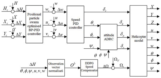
Figure 1.
Landing Control Structure with Speed Compensator.
In the RPM control channel, the control quantity is jointly determined by two parts: one part is the RPM change output by the RPM compensator, and the other part is the rated RPM of the rotor. As a result, the speed control quantity is always up and down around the rated speed . This ensures stability of the speed change. is an offset command output by the neural network, ranging between . The final control command is calculated as , which remains within the physically permissible range at all times.
The RPM compensator is designed using an advanced deep deterministic policy gradient (DDPG) algorithm. This algorithm combines the advantages of deep learning and deterministic policy gradient, which makes the RPM compensator have strong learning and adaptive capabilities. During actual operation, the RPM compensator receives normalised information about the current state of the UAV, including multi-dimensional data such as altitude, speed and attitude. By analysing and processing these data in real time, the RPM compensator is able to accurately calculate the required amount of RPM change and output it to the RPM control channel.
Through this design, the rotational speed compensator not only achieves real-time control of the rotor speed of the UAV, but also effectively optimises the altitude control performance of the UAV. In the actual landing process, this highly integrated and intelligent control system will help to improve the accuracy and safety of the landing and provide a strong guarantee for the smooth landing of the UAV.
3.2. Intensive Study of Relevant Theories
3.2.1. Concepts of Reinforcement Learning
Reinforcement learning is a unique machine learning method that does not require pre-labelled datasets, but instead uses reward signals to instruct an intelligent body to learn a task autonomously. Unlike traditional machine learning where independent samples are trained, samples in reinforcement learning have temporal relationships and interconnections. Intelligent bodies need to select actions based on the current state and objective function, and adjust their behavioural strategies by maximising long-term cumulative rewards. To solve the correlation and variance problems, reinforcement learning employs techniques such as experience replay and goal networks to improve the training effect. Experience playback uses past experience to form more representative training data, while objective networks adjust the objective function to guide the learning process of the intelligent body.
The reinforcement learning model views the learning process as an intelligent body exploring the learning environment, and its basic model is shown in Figure 2. In reinforcement learning, the intelligent body selects an appropriate action to be delivered to the environment according to the current strategy by observing the state of the environment at the current moment. After receiving the action , the environment will generate a new state according to the state transfer matrix. At the same time, the environment will pass a reward signal to the intelligent body, which represents the effect of the intelligent body taking action in the current state.
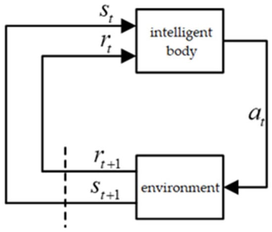
Figure 2.
Reinforcement Learning Interaction Process.
The intelligent body adjusts its strategy through the received reward signals in order to be able to take actions that are more favourable for obtaining positive rewards when it encounters a similar state. In the process of adjusting its strategy, the intelligent body combines the current state of the environment with its own strategy in order to decide its next action. In this way, the intelligent body can gradually optimise its own behavioural strategies in the process of continuously interacting with the environment to achieve the goal of learning.
In summary, reinforcement learning is a learning method that allows an intelligent body to achieve optimal goals by adjusting behavioural strategies as it interacts with its environment. This approach emphasises the learning of the intelligent body in exploring the environment and adjusting strategies through reward signals, enabling the intelligent body to take actions that are more conducive to obtaining positive rewards when it encounters a similar state.
3.2.2. Components of Reinforcement Learning
- Reward is an important measure of the effectiveness of an intelligent body’s actions in a given environment. Reinforcement learning assumes that all decision-making problems can be viewed as problems of maximising cumulative rewards, because intelligences need to learn how to take optimal actions to obtain long-term rewards by interacting with the environment. Intelligentsia learn by trial and error based on the reward signals given by the environment and gradually improve their decision-making ability. In conclusion, rewards play a key role in reinforcement learning and are the basis for intelligent body behavioural feedback and learning.
- Intelligence and environment. They are two core concepts in reinforcement learning, and they interact with each other to form the basic framework of reinforcement learning. From the perspective of the intelligent body, at time the intelligent body firstly observes the state of the environment, which is the perception of the intelligent body to the environment, and it contains all kinds of information about the environment. The intelligent body needs to make an action based on this state, which is the intelligent body’s response to the environment and it will change the state of the environment. After executing this action in the environment, the intelligent body will get a reward signal returned by the environment . The reward signal is the evaluation of the intelligent body’s action by the environment. In reinforcement learning, the interaction between the intelligent body and the environment is a continuous process. The intelligent body makes actions by observing the state of the environment and then adjusts its behaviour according to the feedback from the environment in the expectation of maximising the cumulative rewards over a long period of learning. This process is the core idea of reinforcement learning: the intelligent body learns how to make optimal behaviours through interaction with the environment.
- State. This includes states at the environment, intelligence, and information levels. The environment state is a specific depiction of the environment in which the intelligent body is located, including the data that needs to be observed at the next moment and the data related to the generation of the reward signal , among others. Intelligentsia are not always fully aware of all the details of the environment state, and sometimes this data may contain redundant information. The state of an intelligent body describes the internal structure and parameters, including relevant data used to determine future actions such as network parameters, policy information, etc. The information state, also known as the Markov state, is the sum of all the data that has been useful to the intelligences in history. It reflects the experience and knowledge accumulated from past learning and decision making and becomes an important basis for decision making. In conclusion, state is an essential and important component of AI systems that influences behaviour and decision making, and measures learning effectiveness.
- Strategies. A policy is the basis on which an intelligent body chooses an action in a given state, and it determines how the intelligent body behaves. A strategy is usually represented as a mapping from states to actions and can be a simple rule, function or complex algorithm. Strategies can be categorised as deterministic or stochastic based on whether they contain randomness or not. A deterministic strategy always outputs the same action in a given state, while a stochastic strategy selects different actions based on a certain probability distribution. The stochastic strategy helps the intelligent body to maintain a certain degree of diversity when exploring unknown environments and avoid falling into local optimal solutions.
- Reward function. Reward function is a function that generates reward signals according to the state of the environment, reflecting the effect of the action of the intelligent body and the completion of the goal. In strategy adjustment, the reward function is an important reference basis. The reward signal measures how well the intelligent body chooses an action, and is usually expressed as a numerical value, with larger values indicating greater rewards. For stability, the reward signal is generally adjusted between −1 and 1. Reinforcement learning maximises the cumulative reward value by responding to the reward signal. Intelligentsia need to continuously adjust their action strategies based on real-time reward signals. However, a reward function that is reasonable, objective and applicable to the current task can provide an effective reference and guide the intelligent body towards the optimal solution.
- Value function. The value function is different from the reward function that evaluates the new state directly, but evaluates the current strategy from a long-term perspective, so the value function is also called the evaluation function. The value of state in reinforcement learning is the expectation of the cumulative reward received by the intelligent after performing a series of actions in state , denoted as .
For example, defining as the sum of the reward values of all future states, after the action of the discount factor , can be expressed as Equation (10).
The function can be referred to as a state-value function, and represents the cumulative reward from choosing an action using the strategy , starting from the state . There is another evaluation function as the function, which represents a set of state-action pairs that are evaluated for a given strategy-specific state-specific action.
function: denotes the expectation of the discounted reward sum for the subsequent use of the strategy to select an action for execution after the execution of action in state , as shown in Equation (11).
- Environment Modelling. The environment model in reinforcement learning is an optional part that is used to model how the environment behaves. The environment model consists of two main parts: the reward function and the state transfer function. The reward function is used to determine how good or bad it is to perform an action in a defined state, while the state transfer function determines the next state based on the current state and action.
- Markov Decision Process. Markov Decision Process (MDP) in Reinforcement Learning is a mathematical model for describing the interaction between the environment and the intelligences. MDP assumes that the environment has Markovianity, i.e., the future state of the environment is only related to the current state and not to the past state, or there is no difference between referring to the historical state information and ignoring out the historical information to produce a new state as shown in Equation (4), where the right side of the equation can be represented by the left side of the equation representation. This assumption simplifies the complexity of the problem and allows the reinforcement learning algorithm to handle it more efficiently.
A finite Markov decision process can be represented by a quintuple , where is the non-empty set of all possible states of the system, with denoting the state at moment ; denotes the set of actions, the non-empty set of all possible actions in the system, ; denotes the transfer probability function, denoted as , which is a function that describes the probability of transferring to the next state after executing an action in the current state ; denotes the reward function, denoted as , which is also a function that defines the immediate reward that the intelligence receives after executing a certain action in a specific state; and denotes the objective function, which is usually a value function or a function.
3.3. Deep Deterministic Policy Gradient
DDPG is particularly well suited for solving problems in continuous action spaces. The success of DDPG is largely attributed to its fusion of two previously important algorithms: the DQN (Deep Q-Network) and the DPG (Deterministic Policy Gradient).
DQN is a milestone in the field of Deep Reinforcement Learning, which for the first time successfully combines deep neural networks with Q-Learning algorithms. In Q-Learning, an intelligent learns a strategy by estimating the Q-value (i.e., expected return) of each state-action pair. However, traditional Q-Learning methods encounter difficulties when dealing with high-dimensional state spaces, as this requires the creation of a large table of Q-values. DQN solves this problem by approximating the Q-value function using deep neural networks. In addition, DQN introduces Experience Replay, a technique that stabilises the learning process and improves efficiency as it allows the intelligence to be trained by randomly sampling from stored historical experience.
Unlike many traditional reinforcement learning algorithms, which typically output a probability distribution of actions in a given state, DPG learns a deterministic policy, i.e., it always outputs the same action in a given state. This deterministic strategy may be more effective in some problems as it avoids randomness in action selection. DPG directly optimises the expected returns by gradient ascent, thus updating the strategy parameters. In addition, DPG is combined with an Actor-Critic architecture, where the Actor network is responsible for generating actions and the Critic network is responsible for evaluating the value of these actions.
DDPG combines the advantages of DQN and DPG. It uses deep neural networks to approximate action-value functions (Critic) and deterministic policies (Actor), just like DPG. Also, DDPG introduces the empirical playback technique in DQN to improve data utilisation and stability. In addition, DDPG employs the concept of goal networks, another important technique borrowed from DQN, for stabilising the learning process. By combining these techniques, DDPG is able to achieve efficient and stable learning in a continuous action space.
The internal network components and functions of the DDPG algorithm are as follows:
- Actor current network: this is a policy network that is responsible for generating actions based on the current state. It receives the state as input and outputs a deterministic action through a neural network. The goal of the Actor current network is to maximize the cumulative rewards, learn and optimize the strategy by interacting with the environment.
- Actor target network: this is a copy of the Actor’s current network and is used to stabilise the learning process. Its weights remain constant during training but are updated periodically from the Actor current network. The Actor goal network provides a stable goal for training and helps to reduce oscillations in the learning process.
- Critic Current Network: this is a value network that is responsible for assessing the value of actions taken in the current state. It receives the state and action as inputs and outputs a Q-value through a neural network. The Critic Current Network learns and optimises the value function by interacting with the environment to more accurately assess the value of the action.
- Critic target network: this is a copy of the Critic current network, also used to stabilise the learning process. Its weights remain constant during training, but are periodically updated from the Critic current network. The Critic target network provides a stable target Q value for training, helping to reduce fluctuations in value estimates.
These four networks collaborate with each other to realise the functions of the DDPG algorithm: the Actor current network generates actions based on the current state and interacts with the environment; the Critic current network evaluates the Q-value of the actions taken in the current state and provides gradient information to the Actor current network to guide its optimisation strategy; the Actor goal network and the Critic goal network provide stable goals and Q-values for training, respectively. and Critic goal networks provide stable goals and Q-values, respectively, to help reduce oscillations and fluctuations in the learning process.
Through continuous iteration and learning, the Actor current network and the Critic current network gradually approach the optimal policy and the true value function, thus improving the performance of the algorithms.
Actor’s current network has network parameters , and the input to its neural network is the current state in which the intelligent is in, and the selection of the action is performed through a deterministic policy function, as shown in Equation (13).
In addition, in order to balance the trade-off between exploration and exploitation, DDPGs typically introduce a degree of stochastic noise on the output of a deterministic strategy. This introduction of noise transforms the otherwise deterministic action selection process into a stochastic process. Specifically, after the Actor network generates a deterministic action, a random noise N is added to obtain an action with noise. The intelligent body actually outputs the behaviour by sampling the noisy actions. This strategy of adding random noise essentially constitutes an exploratory strategy that encourages the intelligent body to explore more extensively in the environment. By randomly perturbing the deterministic strategy output, the intelligent body has the opportunity to try out different behaviours and gather more diverse empirical data. This helps to prevent the intelligent body from falling into local optimal solutions prematurely and promotes it to explore effectively in the whole state space. Its exploration strategy is shown in Equation (14).
After an intelligent body selects an action through the Actor’s current network, it receives the reward value and the next state . These experience data, including state, action , reward and next state , are stored as samples in the experience pool. When the experience pool accumulates enough data, the algorithm draws a random batch of samples from it for training. These randomly selected samples are used to update the four network parameters of DDPG. In this way, the intelligences are able to learn and improve their decision-making strategies.
In Critic current networks, the calculation of the Q-value of the parameter is performed iteratively, usually using the Bellman equation with the expression shown in Equation (15):
Once the values of the Actor current network and Critic current network are obtained, the DDPG algorithm uses the Actor target network and Critic target network to update the parameters of these two current networks. Here the gradient descent method is used to update the parameters with the following expression:
The expression for is Equation (17):
Using the above expression, we can calculate the gradient of Critic’s current network and optimise its parameter using gradient descent. At the same time, we introduce a U function to evaluate the performance of Actor’s current network parameters, defined by Equation (18).
The goal of training the Actor’s current network is to maximise the value of this U-function, i.e., to maximise the gain. To achieve this goal, we need to find a deterministic strategy, which can be expressed as follows:
In order to find the optimal parameters of this network, the gradient descent method is used to solve the problem with the following expression:
In addition, we can use the Monte Carlo method to substitute the actual data from the empirical pool into the formula to obtain an unbiased estimate of the calculated expectation. This can be expressed by the following equation:
After obtaining the gradient of the Actor’s current network, we use gradient descent to update its parameter .
The DDPG algorithm adopts a ‘soft’ updating method to gradually optimise the parameters of the Critic and Actor target networks, which is in contrast to the ‘hard’ updating method commonly used in traditional algorithms such as DQN. The ‘soft’ update strategy slightly adjusts the parameters of the target networks at each step, instead of making a large number of updates at once after a fixed number of steps. In this process, the current network is responsible for evaluating the current state and actions in real time and outputting the corresponding policy. The target network, on the other hand, plays a relatively stable reference role for calculating the loss and updating the parameters of the current network accordingly. Although the two networks are structurally consistent, their parameters are different, and the core idea of the ‘soft’ update of the DDPG algorithm is to avoid sudden and drastic changes by smoothly fine-tuning the parameters of the target network at each step. This updating method helps to improve the stability and learning efficiency of the algorithm. The updating process of the parameters and of the Critic and Actor target networks is shown in the following equations:
In summary, the DDPG algorithm flow is illustrated in Figure 3.
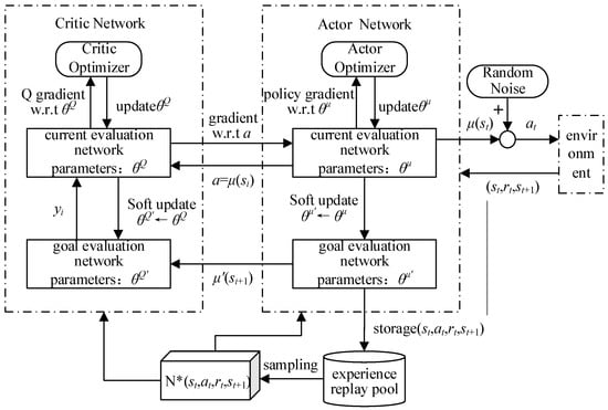
Figure 3.
DDPG algorithm flowchart.
The stability of DDPG is ensured by the target network, experience replay, and deterministic policy gradients. Regarding convergence, under ideal assumptions such as experience replay having exploratory properties and step sizes satisfying relevant conditions, the Critic network can approximately converge to the optimal Q-function. The Actor network converges to a locally optimal policy through unbiased deterministic policy gradients. While strict global convergence cannot be proven due to the nonlinearity of deep neural networks, mechanisms like the target network and experience replay ensure a stable training process that learns effective policies. From a Lyapunov stability perspective, when update steps and target network update rates are appropriately balanced, the system achieves asymptotic stability and converges toward the optimal solution.
3.4. Design of UAV Speed Controller Based on DDPG
3.4.1. Observation Vector Design
The state space should contain the UAV flight state related to the control objective. The control objective of this paper is to optimise the UAV’s altitude control by rotational speed control, to improve the rapidity of the landing, and to improve the smoothness during the landing process. Therefore, the observation information needs to contain the deviation relative to the desired altitude, the UAV’s vertical velocity and the UAV attitude information.
Let the desired height in the geodetic coordinate system be, and the actual height of the UAV in the geodetic coordinate system be; therefore, their height position deviation is:
Let the vertical velocity of the UAV in geodetic coordinates be in the geodetic coordinate system.
The attitude information is supplemented with the sine and cosine values of the pitch, roll and yaw angles in addition to the inputs in the form of pitch, roll, yaw and angular velocities, also with the aim of reducing the complexity of the model to be learnt and making it easier to converge.
In addition, the observation vectors need to be normalised. Because different observation vectors may have different scales and orders of magnitude, if they are not normalised, the model may be affected by the differences in feature scales during training, leading to unstable training or slower convergence. By normalisation, the scale range of all features can be unified and the magnitude differences between features can be eliminated, making it easier for the model to learn effective strategies. In this paper, the minimum-maximum normalisation method is used to normalise each observation. Taking pitch angle as an example, the normalised pitch angle is:
The maximum and minimum values for each observation are shown in Table 1 below.

Table 1.
Normalisation parameters and boundary values.
In summary, the observation vector for speed control is designed as:
3.4.2. Reward Function Design
The goal of reinforcement learning is to optimise the in-round cumulative discount reward, and this reward is the only metric for evaluating controller performance. Therefore, when designing the reward function for RPM compensation, one needs to ensure that it is consistent with the control objective and incorporates the following four aspects:
- Improved speed for height tracking
Improving the rapidity of altitude tracking means arriving at the UAV’s altitude as soon as possible near the desired altitude, so the design reward function should incorporate the deviation from the desired altitude:
where is the height deviation reward coefficient, which is negative and takes a value determined by the size of the deviation range. Due to the use of a quadratic cost function form, the reward function does not change significantly as the deviation approaches zero, which makes it difficult to optimise the strategy further. This problem was observed based on actual training results and as a result an additional reward term was added to the height deviation. The rewards are in the form of a gradient-increasing term, with additional rewards whenever the altitude deviation is less than a range, and these rewards are gradually stacked up with the aim of improving the altitude tracking capability of the shipborne unmanned helicopter. The gradient reward graph is shown in Figure 4.
where , , , , and are complementary positional deviation reward coefficients that are positive and have an absolute value greater than to increase the magnitude of the gradient of the reward function in the case of small positional deviations.
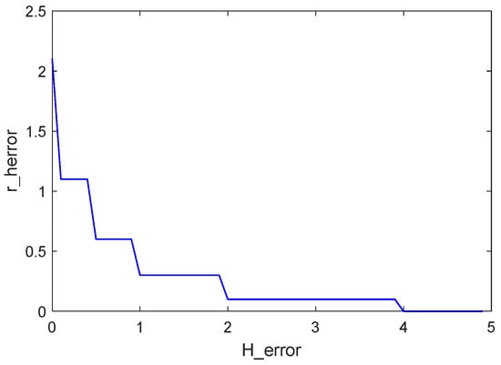
Figure 4.
Gradient-based reward chart.
- 2.
- Improved smoothness of the height tracking process
In order to avoid an overly drastic process of improving the rapidity of altitude tracking, the introduction of velocity and attitude angular rate related bonuses
where and are penalty factors for velocity and attitude angular rate, both of which are negative. These values depend on the magnitude of the angular rate and altitude deviation and the setting of . The introduction of a dynamics-limited reward function term avoids excessive velocity and attitude angular rates during altitude tracking.
- 3.
- Improved smoothness of speed changes
To improve the smoothness of the speed change is to make the main rotor speed not to produce too drastic changes, such as speed jumps, etc., so that it can be maintained in the rated speed up and down, so as to design the reward function contains the speed of the differential component of the speed
where is the penalty coefficient for the rotational speed differential and is negative. The value is taken according to the magnitude of the value.
- 4.
- State constraint
In order to avoid some ineffective exploration, the current turn should be ended when the height error, stance angle and stance angular rate are too large during training to improve the exploration efficiency. At the same time, these rewards are all negative, indicating that continuous exploration will bring continuous negative rewards. If we simply end the round without introducing a penalty mechanism to limit the states that are out of the set range, it is more likely that the intelligent body will choose to make the UAV state out of the constraint range and end the current round before it has learnt good control parameters, thus avoiding the negative rewards from the subsequent position holding and dynamics limitation. The introduction of negative rewards at the end of each round is therefore necessary and motivates the intelligent body to engage in continuous exploration. The specific form is shown below:
where are the maximum values of each state information set in Table 1; is the constraint penalty coefficient, which is negative; and is the difference in distance between the number of steps that have been executed at the end of the round, , and the maximum number of round steps set, , i.e.,
where
is the total number of steps in the round, is the maximum simulation duration of a single round, is the single recursive time step, and is a rounding operation indicating the maximum integer fraction of not exceeded. Such a setting makes it so that when a round ends early, the intelligent is also subject to all the penalties of subsequent poor control performance, inhibiting its tendency to over constrain the state to end the round.
However, this intuitive idea raises a problem: the reward function does not only depend on the observation (state), but is also affected by the number of rounds remaining for early termination. As an example, if the intelligent terminates two rounds early in the same state, but with 100 remaining steps in one round and 50 remaining steps in the other, the former receives twice as much reward as the latter. However, in both cases, the states are the same, which may interfere with value function learning. At the same time, determining the reward by constraining the state is simply a matter of ensuring that the cost associated with early termination is greater than the cost incurred by continued exploration, and thus the in Equation (30) can be replaced with the total number of steps in the round, , which is
In summary the total reward function is obtained in the form
The correlation coefficients in the reward function are shown in the Table 2 below.
Table 2.
Relevant parameters in the reward function.
Where serves as the base height deviation reward coefficient, balancing the reduction in height difference with the gradient reward effect space. Its value is determined based on the deviation range and incorporates an additional reward term for height deviation. The reward structure employs a gradient-incremental approach: whenever the height deviation falls below a certain range, an extra reward is granted, and these rewards accumulate progressively. This mechanism aims to gradually guide the carrier-based helicopter toward a swift landing. to are supplementary positive position deviation reward coefficients. Their absolute values exceed to amplify the gradient magnitude of the reward function when position deviation is small. and represent penalty coefficients for velocity and attitude angular rate, determined by the magnitude of angular rate relative to height deviation and the ah setting. Introducing dynamic constraint reward terms prevents excessive velocity and attitude angular rate during descent. is the penalty coefficient for rotational speed differential components. denotes the constraint penalty coefficient. represents the maximum simulation duration per iteration, while denotes the single-step recursive time step.
3.5. Motion Output
Considering that the output layer of the policy network adopts Tanh activation function, and the output range is (−1,1), set the policy output, which is mapped to the actual control quantity according to the following equation
where , are the maximum and minimum permissible values of the main rotor speed control quantity in UAV flight, respectively. The details are shown in the following Table 3.
Table 3.
Rotor speed boundary value.
3.6. Cognitive Training
- Critic and Actor Network Design
The Critic network and Actor network structures designed in this paper are shown in Figure 5, respectively.
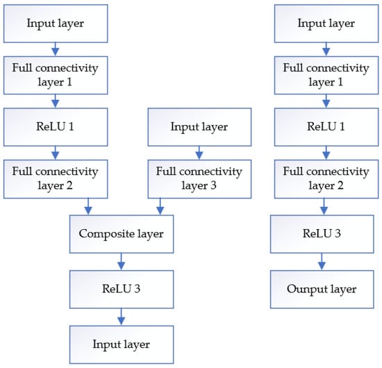
Figure 5.
Critic and Actor network diagrams.
The Critic network uses different paths for observation vectors and action inputs, which are then fused by a combination of layers. Observation vectors are processed by two fully connected layers and one ReLU layer; action inputs are processed by one fully connected layer. The fused features are then nonlinearly transformed by the ReLU layer to output the value assessment. Each fully connected layer contains 200 nodes.
Actor network contains three fully connected layers of 200 nodes each to approximate the optimal policy and output continuous actions. In this, the first and second layers are followed by ReLU activation function, respectively, and the output layer uses Tanh activation function.
- 2.
- Parameterisation
The hyperparameters for the training of intelligences in the DDPG algorithm are shown in Table 4.
Table 4.
Intelligent Body Training Hyperparameters.
- 3.
- Deployment training
The training procedure is built in simulink, and after about 7000 rounds of training the performance of the intelligent body gradually stabilises, the training is stopped, and the strategy network, the value function network and the cumulative rewards for each round are saved. Figure 6 shows the reward change curve of the training process, the light blue is the real cumulative discount reward of each round, and the dark blue solid line is the average of the cumulative discount reward of the neighbouring 250 rounds. The average reward curve smoothes out individual round reward fluctuations and reflects changes in overall performance, as seen in Figure 6, with a single noticeable boost at both 500 and 2000 rounds.
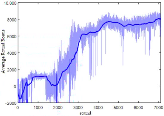
Figure 6.
Round Reward Change Curve.
4. UAV Landing Comprehensive Simulation Experiment
4.1. Highly Controlled Simulation Without Interference
In the absence of airflow disturbances, this paper presents a detailed comparative simulation analysis of the optimisation of the RPM compensator for altitude control. This analysis aims to reveal the performance differences between the variable speed strategy and the constant speed strategy for UAV altitude control.
Firstly, the height controller designed in Chapter 3 was used as the reference object for this simulation. This controller has already shown good performance in previous experiments. Secondly, the height signal is set as shown in Equation (36).
Figure 7 illustrates the simulation results of UAV altitude signal tracking in the absence of interference. During the ascent phase, the UAV with the variable RPM strategy shows a significant advantage. It reaches the altitude of 100 metres quickly and smoothly in only 11.5 s without any overshoot during the whole process. In contrast, the UAV with the constant RPM strategy took a longer 15.36 s to reach the same altitude and experienced a 2 per cent overshoot.
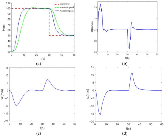
Figure 7.
(a) Comparison diagram of interference free altitude signal tracking; (b) Rotor speed variation curve without interference; (c) Speed variation curve at constant speed without interference; (d) Speed variation curve under interference free variable speed.
The variable RPM strategy also showed its superiority in the descent phase of the comparison. The UAV reached the 50 m altitude in 41.05 s without any overshoot. The UAV with the constant RPM strategy not only took 45.53 s longer to complete the same manoeuvre, but also had significant overshooting, which could have caused the unmanned UAV to hit the deck at a higher speed during landing, resulting in a failed landing.
In addition, Figure 7 show the UAV’s vertical speed profiles for both strategies. The results show that the UAV with the variable RPM strategy is able to increase or decrease its vertical speed faster with the RPM compensator. This means that the variable RPM strategy can provide the UAV with higher manoeuvrability and agility when faced with unexpected situations or missions that require fast response.
Through this simulation analysis, we clearly see the remarkable effect of the RPM compensator in optimising the altitude control of the UAV. In the absence of airflow disturbance, the variable RPM strategy provides a more advanced and effective solution for UAV altitude control with its fast, smooth and accurate performance.
4.2. Simulation of Altitude Control Under Air Turbulence
In order to analyse the anti-disturbance performance of the rotational speed compensator in terms of altitude control, the airflow disturbance described in Section 2 is introduced in the simulation. In this simulation, we continue to use the altitude controller introduced in Section 3 as the reference object to ensure the consistency and accuracy of the analysis.
Figure 8 demonstrates the performance of the variable RPM strategy and the constant RPM strategy in tracking the altitude signals in the presence of imposed airflow perturbations. The results show that even in the presence of significant perturbations, the variable RPM strategy still exhibits significant advantages in terms of rise time and amount of overshoot. In particular, when the UAV is steadily maintained at 100 m altitude, we observe altitude fluctuations in the range of −0.5 m to 0.5 m under the variable RPM strategy, while the fluctuations under the constant RPM strategy are relatively large, reaching −2 m to 2 m. The results show that the altitude fluctuations under the variable RPM strategy are in the range of −2 m to 2 m.
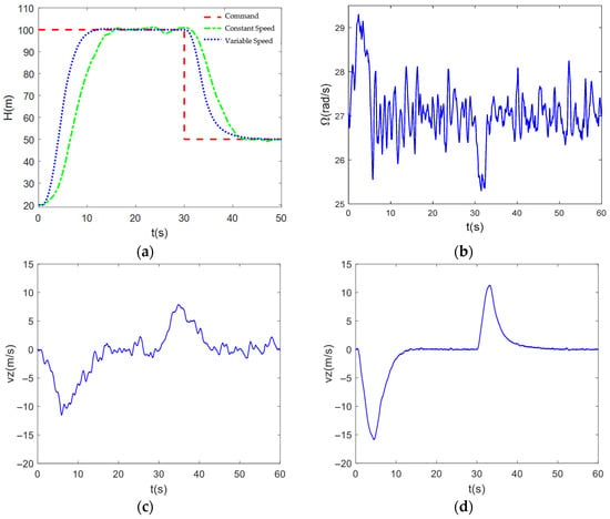
Figure 8.
(a) Comparison diagram of height signal tracking under airflow disturbance; (b) Speed variation curve under interference; (c) Speed variation curve under constant speed with interference; (d) Speed variation curve under interference and variable speed.
In addition, Figure 8 show the vertical velocity profiles of the UAV under the two strategies. Through the comparative analysis, we can clearly see that by introducing the RPM compensator, the UAV is able to effectively counteract the changes in the velocity direction caused by the airflow disturbance. Under the variable RPM strategy, the vertical velocity change of the UAV is smoother and more controllable, which is attributed to the precise adjustment and fast response of the RPM compensator. In contrast, the vertical velocity under the constant RPM strategy shows greater fluctuation and uncertainty.
In summary, the rotational speed compensator designed in this paper demonstrates a strong anti-disturbance capability in altitude control. By precisely adjusting the rotational speed of the UAV to compensate for the influence of external disturbances, the compensator significantly improves the stability and control accuracy of the UAV in a complex airflow environment.
To further illustrate the advantages of the algorithm designed in this paper, we systematically compare the proposed control strategy with current mainstream advanced control methods. The MPC’s prediction time horizon is set to 20 steps, and the control time horizon is set to 10 steps. The constraints are given by Equation (37).
The constraints in Equation (37) are as follows: Initial condition constraint: It stipulates that the starting point of the prediction must be the system’s current actual state. State equation constraint: This constraint defines the dynamic model that the system state prediction must follow. Torque constraint: This constraint defines the relationship between the system’s predicted output and the predicted state. State constraint: This constraint imposes upper and lower limits on the system’s state variables. Control input constraint: The magnitude of the control input must always remain within its permitted maximum and minimum ranges.
As shown in Figure 9, we have added comparison curves with model predictive control methods in the simulation results. The results demonstrate that the DDPG method exhibits superior dynamic response and rapidity.
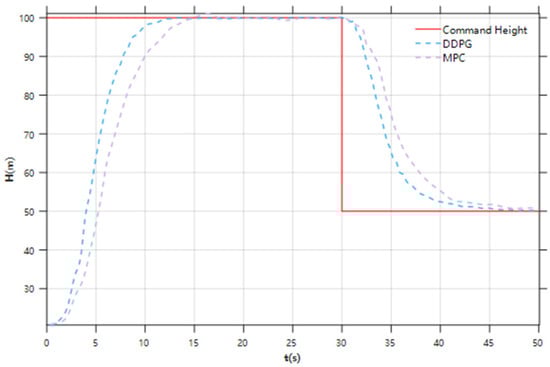
Figure 9.
Simulation Diagram of Height Controller Under Different Methods.
4.3. Linear Trajectory Tracking Experiment
For deck motion prediction, this paper employs an online LSTM deck motion estimator. LSTM is a specialized recurrent neural network designed specifically for processing time-series data. Compared to traditional neural networks, LSTM demonstrates faster convergence and higher accuracy when handling sequential problems. During this study, the LSTM model was initially trained using an offline training approach. This approach involves training the model in a single batch after collecting all relevant data, rather than processing data streams in real time. This method offers the advantages of comprehensive control over the training process and enhanced efficiency. Offline training validated the feasibility of the LSTM model for deck motion prediction, and its predictive performance was evaluated by comparing results with actual motion data. If the prediction results are satisfactory, an online deck motion estimator is designed for practical application. The online deck motion estimator must consider factors such as accuracy, real-time capability, and stability. These aspects are thoroughly addressed during the design process to ensure performance, with continuous optimization and adjustments made to adapt to environmental and demand changes. As the sliding window moves to the right, each step generates a corresponding set of input samples and output samples. These samples are then used to train the model, enabling it to learn how to predict output data based on input data.
The ship’s linear motion trajectory formulae used in this paper are as follows:
where , , and are the displacements in the x, y, and z directions produced at the ideal landing point as affected by the deck motion.
At the moment , the UAV is in a hovering state not far from the ship, the initial position is (0, 0, 10), the initial position of the ship is (0, 0) in metres, and the initial speed is (5, 0) in metres per second. At the beginning of the simulation, the UAV hovers and follows up, then receives the deck motion prediction data into the control system, the UAV adjusts its attitude, follows the ideal landing point on the ship and waits for the rest period until the ‘rest period’ appears. Finally, the ‘resting period’ of the deck movement is found, and the UAV then enters the landing phase. The linear trajectory tracking effect is shown in Figure 10. The distance errors in various directions and the velocity curve during the landing process are shown in Figure 11. The contact point location diagram is shown in Figure 12.
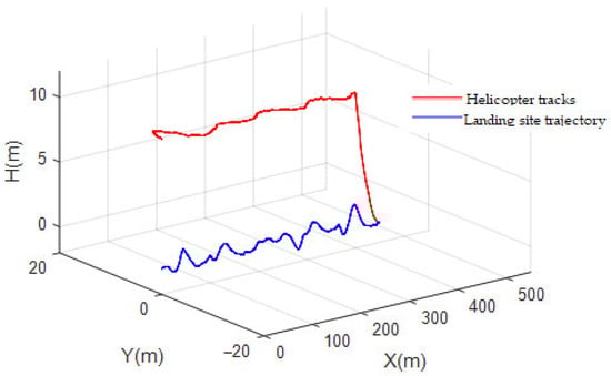
Figure 10.
Linear trajectory tracking diagram.
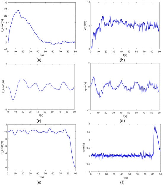
Figure 11.
(a) Longitudinal distance error curve; (b) Longitudinal velocity curve; (c) Lateral distance error curve; (d) Lateral velocity curve; (e) Height distance error curve; (f) Vertical velocity curve.
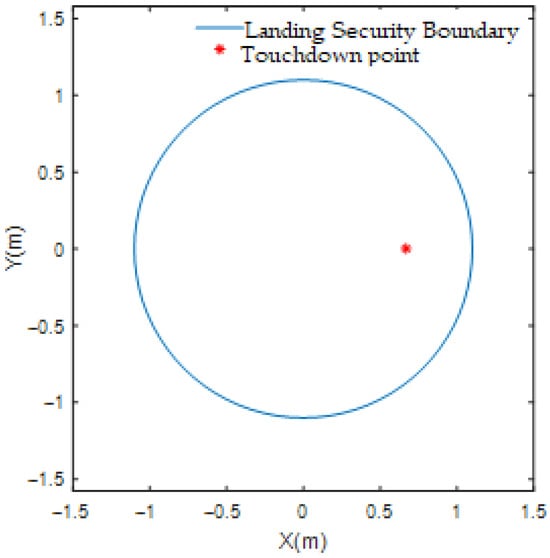
Figure 12.
Linear trajectory tracking touchdown point location map.
From the figure, it can be seen that the landing controller designed in this paper has better control in high sea state.
4.4. Circular Trajectory Tracking Experiment
The equations for the ship’s trajectory are shown below:
The initial position of the ship is (100, 0) when = 0 from the equation.
The initial position of the UAV is set to (0, 0, 10) and it is made to hover. At the beginning of the real time, the UAV hovers to follow, then receives the deck motion prediction data into the control system, the UAV adjusts its attitude to follow the ideal landing point on the ship, and waits for the rest period until the ‘rest period’ appears. Finally, the ‘resting period’ of the deck movement is found, and the UAV then enters the landing phase. The linear trajectory tracking effect is shown in Figure 13. Figure 14 shows the distance error and velocity in each direction during circular trajectory tracking. Figure 15 illustrates the heading angle error. Figure 16 depicts the position of the contact point during circular trajectory tracking.
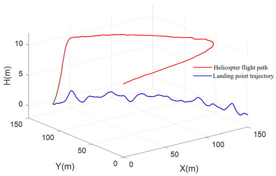
Figure 13.
Circular trajectory tracking diagram.
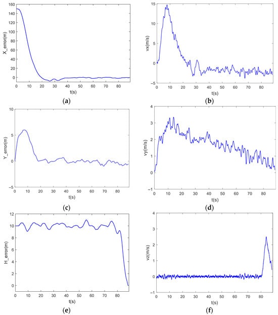
Figure 14.
(a) Longitudinal distance error curve; (b) Longitudinal velocity curve; (c) Lateral distance error curve; (d) Lateral velocity curve; (e) Height distance error curve; (f) Vertical velocity curve.
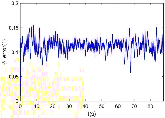
Figure 15.
Heading Angle Error Chart.
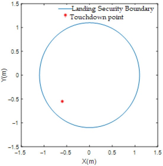
Figure 16.
Circular trajectory tracking touchdown point location map.
As shown in the figure, the ship landing controller designed in this paper is still able to complete the ship landing task under the situation of air current disturbance and wide range of ship’s heading change. For algorithm real-time performance, we selected the NVIDIA Jetson Orin platform—widely adopted in the industry for high-end unmanned system development—as our target hardware environment. We deployed DDPG on this platform and conducted over 10,000 timed tests of its inference process. The maximum average duration was 40 ms, with an average of approximately 20 ms, meeting the fundamental 20 Hz control cycle requirement. After appropriate optimization, the DDPG algorithm’s inference process achieves high computational efficiency, satisfying the real-time performance demands for controllers in unmanned aerial vehicle systems. Furthermore, the simulation results above demonstrate that under the current computational settings, the online learning process of this controller meets real-time requirements and achieves the expected rapid response and precise control performance. DDPG integrates the strengths of deep learning and reinforcement learning to enable efficient decision making in continuous action spaces, progressively optimizing control strategies through interactive learning. Compared to traditional control methods, DDPG does not require precise mathematical models and can directly learn optimal compensation strategies from environmental feedback, thereby better addressing uncertainties in vessel motion. Furthermore, this method adapts to complex environments during training and continuously optimizes control performance, significantly enhancing system robustness and convergence speed.
5. Conclusions
In this paper, a comprehensive and in-depth study of shipboard unmanned helicopter landing control technology is carried out from various aspects, such as unmanned helicopter modelling, rotational speed compensator research and deck motion prediction. The modelling of UAV aerodynamic components is systematically carried out, with a focus on the main rotor model. This lays the foundation for the design of the rotational speed compensator in the subsequent chapters. In addition, a deck motion model and an atmospheric turbulence model are established in this paper to more realistically simulate the environmental conditions during UAV landing. The establishment of these models provides strong support for the subsequent simulation experiments and performance evaluation. Aiming at the altitude control optimisation problem during the landing process, this paper designs a speed compensator based on reinforcement learning. The DDPG framework is adopted to ensure the continuity of output and training stability. Accurate control of the UAV RPM is achieved by interacting with the UAV dynamics model through well-designed observation vectors, reward functions and action outputs. After extensive training, the controller converges and exhibits excellent performance. Simulation experiments verify that the addition of RPM compensation results in a significant improvement in altitude tracking performance and better anti-disturbance capability. Finally, a full-flow integrated landing simulation is performed to verify the robustness of the designed system.
Author Contributions
Conceptualization, G.C.; methodology, P.F.; software, G.C., P.F. and X.W.; validation, G.C. and P.F.; writing—review, G.C., P.F. and X.W. All authors have read and agreed to the published version of the manuscript.
Funding
This research received no external funding.
Data Availability Statement
The original contributions presented in the study are included in the article, further inquiries can be directed to the corresponding author.
Conflicts of Interest
The authors declare no conflicts of interest.
References
- Shi, Y.; He, X.; Xu, Y.; Xu, G. Numerical study on flow control of ship airwake and rotor airload during helicopter shipboard landing. Chin. J. Aeronaut. 2019, 32, 324–336. [Google Scholar] [CrossRef]
- Huang, Y.; Zhu, M.; Zheng, Z.; Feroskhan, M. Fixed-time autonomous shipboard landing control of a helicopter with external disturbances. Aerosp. Sci. Technol. 2019, 84, 18–30. [Google Scholar] [CrossRef]
- Horn, J.F.; Yang, J.; He, C.; Lee, D.; Tritschler, J.K. Autonomous ship approach and landing using dynamic inversion control with deck motion prediction. In Proceedings of the 41st European Rotorcraft Forum 2015, Munich, Germany, 1–4 September 2015. [Google Scholar]
- Memon, W.A.; Owen, I.; White, M.D. Motion Fidelity Requirements for Helicopter-Ship Operations in Maritime Rotorcraft Flight Simulators. J. Aircr. 2019, 56, 2189–2209. [Google Scholar] [CrossRef]
- Xia, K.; Lee, S.; Son, H. Adaptive control for multi-rotor UAVs autonomous ship landing with mission planning. Aerosp. Sci. Technol. 2020, 96, 105549. [Google Scholar] [CrossRef]
- Wang, L.; Chen, R.; Xie, X.; Yuan, Y. Modeling and full-speed range transition strategy for a compound helicopter. Aerosp. Sci. Technol. 2025, 160, 110092. [Google Scholar] [CrossRef]
- Song, J.; Wang, Y.; Ji, C.; Zhang, H. Real-time optimization control of variable rotor speed based on Helicopter/turboshaft engine on-board composite system. Energy 2024, 301, 131701. [Google Scholar] [CrossRef]
- Xia, H. Modeling and control strategy of small unmanned helicopter rotation based on deep learning. Syst. Soft Comput. 2024, 6, 200146. [Google Scholar] [CrossRef]
- Dudnik, V.; Gaponov, V. Correction system of the main rotor angular speed for helicopters of little weight categories. Transp. Res. Procedia 2022, 63, 187–194. [Google Scholar] [CrossRef]
- Sun, L.; Huang, Y.; Zheng, Z.; Zhu, B.; Jiang, J. Adaptive nonlinear relative motion control of quadrotors in autonomous shipboard landings. J. Frankl. Inst. 2020, 357, 13569–13592. [Google Scholar] [CrossRef]
- Qiu, Y.; Li, Y.; Lang, J.; Wang, Z. Dynamics analysis and control of coaxial high-speed helicopter in transition flight. Aerosp. Sci. Technol. 2023, 137, 108278. [Google Scholar] [CrossRef]
- Halbe, O.; Hajek, M. Robust Helicopter Sliding Mode Control for Enhanced Handling and Trajectory Following. J. Guid. Control Dyn. 2020, 43, 1805–1821. [Google Scholar] [CrossRef]
- Yuan, Y.; Duan, H. Adaptive Learning Control for a Quadrotor Unmanned Aerial Vehicle landing on a Moving Ship. IEEE Trans. Ind. Inform. 2024, 20, 534–545. [Google Scholar] [CrossRef]
- Shi, Y.; Li, G.; Su, D.; Xu, G. Numerical investigation on the ship/multi-helicopter dynamic interface. Aerosp. Sci. Technol. 2020, 106, 106175. [Google Scholar] [CrossRef]
- Greer, W.B.; Sultan, C. Infinite horizon model predictive control tracking application to helicopters. Aerosp. Sci. Technol. 2020, 98, 105675. [Google Scholar] [CrossRef]
- Di, Z.; Mishra, S.T.; Gandhi, F. A Differential Flatness-Based Approach for Autonomous Helicopter Shipboard Landing. IEEE/ASME Trans. Mechatron. 2022, 27, 1557–1569. [Google Scholar] [CrossRef]
- Huang, Y.; Zhu, M.; Zheng, Z.; Low, K.H. Linear Velocity-Free Visual Servoing Control for Unmanned Helicopter Landing on a Ship with Visibility Constraint. IEEE Trans. Syst. Man Cybern. Syst. 2022, 52, 2979–2993. [Google Scholar] [CrossRef]
- Zhang, Z.; Li, W.; Sun, H.; Wang, B.; Zhao, D.; Ni, T. Research on Reliability Growth of Shock Absorption System in Rapid Secure Device of Shipboard Helicopter. IEEE Access 2023, 11, 134652–134662. [Google Scholar] [CrossRef]
- Liu, M.; Wei, J.; Liu, K. A Two-Stage Target Search and Tracking Method for UAV Based on Deep Reinforcement Learning. Drones 2024, 8, 544. [Google Scholar] [CrossRef]
- Zhang, L.; Peng, J.; Yi, W.; Lin, H.; Lei, L.; Song, X. A State-Decomposition DDPG Algorithm for UAV Autonomous Navigation in 3D Complex Environments. IEEE Internet Things J. 2023, 11, 10778–10790. [Google Scholar] [CrossRef]
- Yu, Y. Multi-Objective Optimization for UAV-Assisted Wireless Powered IoT Networks Based on Extended DDPG Algorithm. IEEE Trans. Commun. 2021, 69, 6361–6374. [Google Scholar] [CrossRef]
- Tian, S.; Li, Y.; Zhang, X.; Zheng, L.; Cheng, L.; She, W.; Xie, W. Fast UAV path planning in urban environments based on three-step experience buffer sampling DDPG. Digit. Commun. Netw. 2024, 10, 813–826. [Google Scholar] [CrossRef]
- Wang, T.; Ji, X.; Zhu, X.; He, C.; Gu, J.F. Deep Reinforcement Learning based running-track path design for fixed-wing UAV assisted mobile relaying network. Veh. Commun. 2024, 50, 100851. [Google Scholar] [CrossRef]
- Barnawi, A.; Kumar, N.; Budhiraja, I.; Kumar, K.; Almansour, A.; Alzahrani, B. Deep reinforcement learning based trajectory optimization for magnetometer-mounted UAV to landmine detection. Comput. Commun. 2022, 195, 441–450. [Google Scholar] [CrossRef]
- Sarikaya, B.S.; Bahtiyar, S. A survey on security of UAV and deep reinforcement learning. Ad Hoc Netw. 2024, 164, 103642. [Google Scholar] [CrossRef]
- Zhang, S.; Li, Y.; Dong, Q. Autonomous navigation of UAV in multi-obstacle environments based on a Deep Reinforcement Learning approach. Appl. Soft Comput. 2022, 115, 108194. [Google Scholar] [CrossRef]
- Trad, T.Y.; Choutri, K.; Lagha, M.; Meshoul, S.; Khenfri, F.; Fareh, R.; Shaiba, H. Real-Time Implementation of Quadrotor UAV Control System Based on a Deep Reinforcement Learning Approach. Comput. Mater. Contin. 2024, 81, 4757–4786. [Google Scholar] [CrossRef]
- Ma, B.; Liu, Z.; Jiang, F.; Zhao, W.; Dang, Q.; Wang, X.; Zhang, G.; Wang, L. Reinforcement learning based UAV formation control in GPS-denied environment. Chin. J. Aeronaut. 2023, 36, 281–296. [Google Scholar] [CrossRef]
- Lu, Y.; Xu, C.; Wang, Y. Joint Computation Offloading and Trajectory Optimization for Edge Computing UAV: A KNN-DDPG Algorithm. Drones 2024, 8, 564. [Google Scholar] [CrossRef]
- Yang, H.; Ni, T.; Wang, Z.; Wang, Z.; Zhao, D. Dynamic modeling and analysis of traction operation process for the shipboard helicopter. Aerosp. Sci. Technol. 2023, 142, 108661. [Google Scholar] [CrossRef]
- Taymourtash, N.; Zagaglia, D.; Zanotti, A.; Muscarello, V.; Gibertini, G.; Quaranta, G. Experimental study of a helicopter model in shipboard operations. Aerosp. Sci. Technol. 2021, 115, 106774. [Google Scholar] [CrossRef]
- Wang, G. Design of Position Control Rate for Unmanned Helicopters During Hovering/Low-Speed Flight Under Atmospheric Disturbances. Master’s Thesis, Nanjing University of Aeronautics and Astronautics, Nanjing, China, 2013. [Google Scholar]
- Beal, T.R. Digital simulation of atmospheric turbulence for Dryden and von Karman models. J. Guid. Control Dyn. 1993, 16, 132–138. [Google Scholar] [CrossRef]
Disclaimer/Publisher’s Note: The statements, opinions and data contained in all publications are solely those of the individual author(s) and contributor(s) and not of MDPI and/or the editor(s). MDPI and/or the editor(s) disclaim responsibility for any injury to people or property resulting from any ideas, methods, instructions or products referred to in the content. |
© 2025 by the authors. Licensee MDPI, Basel, Switzerland. This article is an open access article distributed under the terms and conditions of the Creative Commons Attribution (CC BY) license (https://creativecommons.org/licenses/by/4.0/).