Empirical Evaluation and Simulation of GNSS Solutions on UAS-SfM Accuracy for Shoreline Mapping

Abstract

Uncrewed aircraft systems (UASs) and structure-from-motion/multi-view stereo (SfM/MVS) photogrammetry are efficient methods for mapping terrain at local geographic scales. Traditionally, indirect georeferencing using ground control points (GCPs) is used to georeference the UAS image locations before further processing in SfM software. However, this is a tedious practice and unsuitable for surveying remote or inaccessible areas. Direct georeferencing is a plausible alternative that requires no GCPs. It relies on global navigation satellite system (GNSS) technology to georeference the UAS image locations. This research combined field experiments and simulation to investigate GNSS-based post-processed kinematic (PPK) as a means to eliminate or reduce reliance on GCPs for shoreline mapping and charting. The study also conducted a brief comparison of real-time network (RTN) and precise point positioning (PPP) performances for the same purpose. Ancillary experiments evaluated the effects of PPK base station distance and GNSS sample rate on the accuracy of derived 3D point clouds and digital elevation models (DEMs). Vertical root mean square errors (RMSE_z), scaled to the 95% confidence interval using an assumption of normally-distributed errors, were desired to be within 0.5 m to satisfy National Oceanic and Atmospheric Administration (NOAA) requirements for nautical charting. Simulations used a Monte Carlo approach and empirical tests to examine the influence of GNSS performance on the quality of derived 3D point clouds. RTN and PPK results consistently yielded RMSE_z values within 10 cm, thus satisfying NOAA requirements for nautical charting. PPP did not meet the accuracy requirements but showed promising results that prompt further investigation. PPK experiments using higher GNSS sample rates did not always provide the best accuracies. GNSS performance and model accuracies were enhanced when using base stations located within 30 km of the survey site. Results without using GCPs observed a direct relationship between point cloud accuracy and GNSS performance, with ${\mathrm{R}}^2$ values reaching up to 0.97.

1. Introduction

Small uncrewed aircraft systems (UASs) equipped with digital cameras provide efficient and affordable means for mapping terrain at localized geographic scales. This technique is called structure-from-motion/multi-view stereo (SfM/MVS) photogrammetry [1,2,3], or UAS-SfM, and has reduced both the time and human labor needed to monitor local topographies in natural environments. UAS-SfM has benefited various applications, including coastal and civil engineering, land cover classification, and the generation of digital twins [4,5,6,7,8]. UAS-SfM is particularly relevant to coastal surveying and engineering because of its potential to complement or replace traditional surveying methods for monitoring coastal processes and improve data collection efficiency and temporal coverage [9,10]. Use cases include beach volume quantification and post-disaster assessments [11,12], identification and extraction of shoreline and foredune position [13], frequent monitoring of overall beach/coastal topography [14,15], and close-range observation of hurricane dynamics [16]. UAS-SfM has been found to generate mapping products consistent with publicly available datasets while enhancing the decision-making process associated with data collection [13,15]. When deployed effectively over local geographic areas, UAS-SfM can generate high-resolution topographic models of an area of interest with significantly less labor and time resources than conventional surveying methods [17,18,19]. Common topographic models include digital surface models (DSMs) and bare-earth digital elevation models (DEMs), sometimes referred to as digital terrain models (DTMs), which differ mainly in whether or not they capture elevated surface features above the ground [20]. DSMs typically capture elevated features such as buildings, trees, and cars while DTMs normally capture only the bare earth.

The accuracy of UAS-SfM is influenced by factors such as the quality of the UAS platform and camera sensor, image quality, the georeferencing technique used to correct UAS image locations, the precision of corrected image locations, percentage of image overlap, topographic features, wind, and the height at which the UAS is flown [21,22,23,24,25,26,27]. Traditionally, a ground control point (GCP) network is used for the georeferencing task through a process known as indirect georeferencing or aerotriangulation [28]. Indirect georeferencing requires three or more GCPs for camera calibration and constrainment of derived mapping products, and has been reported to achieve vertical accuracies within a few centimeters [29,30,31]. However, using GCPs can be impractical or cost-prohibitive, particularly in remote or inaccessible locations, and leads to lengthy field data collection and post-processing workflows. Herein lies the motivation for this study: to explore GCP-free techniques for mapping coastal shorelines with UAS-SfM. Direct georeferencing is an alternative that uses onboard global navigation satellite system (GNSS) technology, sometimes integrated with an inertial measurement unit (IMU) for measuring orientation, to enable tracking of the UAS position throughout its deployment [32], thereby allowing for the georeferencing of image locations. This can be achieved autonomously, without implementing additional GNSS correction procedures, or using advanced differential correction techniques such as real-time kinematic (RTK), post-processed kinematic (PPK), and precise point positioning (PPP), depending on the application for which they are used, GNSS data availability, and desired accuracies [30,32,33].

Single-base RTK uses two receivers (i.e., a base and a rover) that collect simultaneous GNSS data from available satellites to provide immediate geopositional solutions [34]. A similar concept, real-time network (RTN), also provides real-time GNSS solutions but relies on a network of GNSS reference stations in the vicinity of the survey site instead [35]. The terms RTN and network RTK (or NRTK) have been used interchangeably in the literature. A limitation of these real-time approaches is their increased susceptibility to errors resulting from loss of communication between the base station and the rover receiver. Some studies have addressed the challenges associated with communication loss in real-time GNSS correction techniques [36,37]. In the case of RTN, there may be instances where the network of reference stations lacks coverage within the survey area. Single-base PPK also uses two GNSS receivers for positional corrections but requires additional post-processing of UAS trajectories after the survey [38]. The base station used for PPK corrections can either be a temporary station occupied by a GNSS receiver (e.g., static GNSS), or a semi-permanent station that continuously logs GNSS information (e.g., continuous operating reference stations (CORSs)). PPP undergoes corrections for ambiguities related to ephemerides and clock data [39]. This approach is convenient for mapping shorelines and remote areas because it requires no base station for differential GNSS corrections [40,41]. However, it is also more prone to limitations such as the long convergence times required to achieve accurate results and the occasional inability to access online services due to website maintenance or being out of service [42,43,44].

Some of the factors that affect the performance of GNSS and direct georeferencing discussed in the literature include the quality of the GNSS receiver, the accuracy of the synchronization between the time of capture and image geotags, and GNSS-related atmospheric biases (i.e., ionospheric and tropospheric refraction) [45,46,47,48]. Several studies have shown that using multi-frequency GNSS receivers, instead of single-frequency receivers, often improves the performance of direct georeferencing techniques, in both static and kinematic modes [34,40,44]. It has also been observed that higher GNSS accuracies are often achieved in static mode compared to kinematic. Ref. [49] compared both approaches and obtained centimeter-level accuracies in static mode and decimeter-level in kinematic.

The impact of different GNSS correction techniques on UAS-SfM has also been addressed in the literature. One study explored direct and indirect georeferencing techniques and reported a vertical accuracy (i.e., root mean square error (RMSE_z) relative to independently surveyed checkpoints) of 0.03 m for indirect georeferencing, between 0.24 m and 0.36 m for PPK-only corrections, and 4.21 m for uncorrected UAS trajectories [30]. The difference in accuracy between the two PPK methods was attributed to one of the PPK systems being more advanced, which further minimized distance-dependent errors thus improving accuracies. A second study compared the accuracies of RTK, RTN, and indirect georeferencing techniques [50]. The study reported an average RMSE_z of 4.6 cm for RTK, 9.5 cm for RTN, and 2.0 cm for indirect georeferencing. The combined approach (i.e., direct + indirect georeferencing) resulted in average RMSE_z values of 2.7 cm for RTK + 1 GCP and 3.7 cm for RTN + 1 GCP. Another study used UAS-SfM for the kilometer-scale topographic mapping of a river channel [51]. The study argued that GCPs are not necessary for topographic mapping at kilometer scales. In their experiment, using five GCPs increased the RMSE_z (relative to 3300 independent checkpoints) by 6 mm compared to a no-GCP instance. In a different study, RTK and PPK were highlighted as the only systems capable of providing repeatable and highly accurate UAS-SfM solutions without using GCPs [52].

Most analyses of GNSS effects on UAS-SfM accuracy rely on field experiments to draw meaningful conclusions. However, simulations can also be applied to examine such effects. Previous work has leveraged Monte Carlo simulations to evaluate the relationship between two or more variables by observing how changes in one of the variables affect the rest [53]. These simulations provide informative and streamlined answers to specific questions without the burden of time-consuming workflows and exposure to dangerous situations that may occur with in situ fieldwork measurements [54,55]. An example is provided in [56], where researchers used a Monte Carlo simulation to iteratively quantify the precision of a UAS-SfM-derived 3D point cloud as a result of changes in the camera model.

While GNSS and UAS-SfM technologies have proven valuable for mapping the position and elevation of shorelines, challenges remain in optimizing data collection workflows. This study explores ways to minimize reliance on indirect georeferencing techniques using GCPs without compromising the accuracy of UAS-SfM mapping products. The rest of this paper is organized as follows: Section 2 outlines the purpose and core contributions of this study; Section 3 provides an overview of the study sites; Section 4 discusses the methods and techniques used; Section 5 presents the results; Section 6 discusses the implications and significance of the results obtained; and Section 7 concludes the paper and provides future directions.

2. Study Purpose and Objectives

This study stems from a project with the U.S. Office of Coast Survey, a Program Office of the National Ocean Service (NOS) within the National Oceanic and Atmospheric Administration (NOAA), and focuses on the impact of different GNSS trajectory solutions on the vertical accuracy of UAS-SfM-derived 3D point clouds and inherent digital surface/terrain models. The project sought to investigate whether these GNSS techniques can be used to eliminate or reduce the use of GCPs while meeting NOAA standards for nautical charting. When surveying exposed land surfaces or submerged features up to 100 m in depth, NOAA requires vertical accuracies within 0.5 m at the 95% confidence level [57]. This study expands on the work presented in [58] and provides the following core contributions:

• Evaluation of PPK and brief experimentation with RTN and PPP GNSS trajectory solutions as alternatives to GCPs for the direct georeferencing of UAS-SfM image locations and derived mapping products;
• Assessment of UAS-SfM data product vertical accuracy as a result of PPK GNSS sample rate, fix percentage, and baseline distance;
• Comparison of UAS-SfM-derived products against ground control data acquired using other surveying techniques (i.e., RTN GNSS, total station, and geodetic-grade terrestrial light detection and ranging (lidar));
• Application of Monte Carlo simulation techniques to examine the impact of GNSS quality on the vertical accuracy of UAS-SfM-derived point clouds.

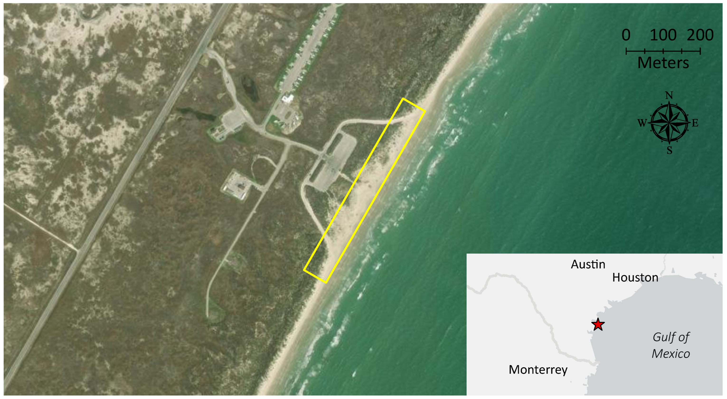
By integrating empirical field testing and situations into performance and accuracy assessments, this study explores how UAS-SfM, when combined with different GNSS correction methods, can enhance data collection efficiency and enable high-precision survey work in remote and inaccessible shoreline areas. In turn, shoreline mapping activities along coastal regions can be conducted using UASs deployed from ships to accurately map various exposed landforms and shorelines at the required NOAA accuracies.

3. Study Sites

This research considered three different study sites in the United States, surveyed between 23 March 2021 and 13 July 2021. The sites were selected strategically based on their relevance to the objectives of this research. The first site, Mustang Island State Park (Figure 1), is a wave-dominated pedestrian beach along the southern Gulf Coast of Texas. The area of interest spanned approximately 1000 m alongshore and 50 m cross-shore, covering roughly 0.050 km². This site was selected because of its coastal characteristics, typified by fine beach sand and low vegetation. The study focused on a pedestrian-only section of the beach, ensuring no vehicular interference during data acquisition. In addition, the research team had existing permits for UAS operation and data collection at this location through the Texas Parks and Wildlife Department. The data obtained from this site supported the RTN, PPK, and PPP analyses of the study.

The second site, McNary Field (Figure 2a) is located at Oregon State University. The area of interest encompassed an area of approximately 0.045 km² which featured diverse landscapes, including short and tall vegetation as well as patches of concrete. This second site was selected because it is an extremely well-surveyed and well-characterized site with existing survey control which the research team used for reference during the surveys. The research team also had blanket approvals to use this site for UAS test flights. Finally, data were collected at the Neptune State Scenic Area (Figure 2b), a coastal site in Oregon, characterized by a wave-dominated beach backed by rock outcrops, freshwater outflows, a bridge, vegetated cliffs, cobble, and fine beach sand, all of which could be captured in a single UAS flight. The focus area covered approximately 0.051 km². Despite being a scenic site, this area experienced minimal pedestrian and vehicular presence at certain times, thus allowing for field data acquisition with minimal interference. The research team also had existing permits for UAS operation in this last study site through the Oregon Parks and Recreation Department. Data from the latter two study sites were used to examine the effects of GNSS quality on the vertical accuracy of UAS-SfM-derived point clouds, which also helped to perform a Monte Carlo simulation that further describes this relationship.

4. Methodology

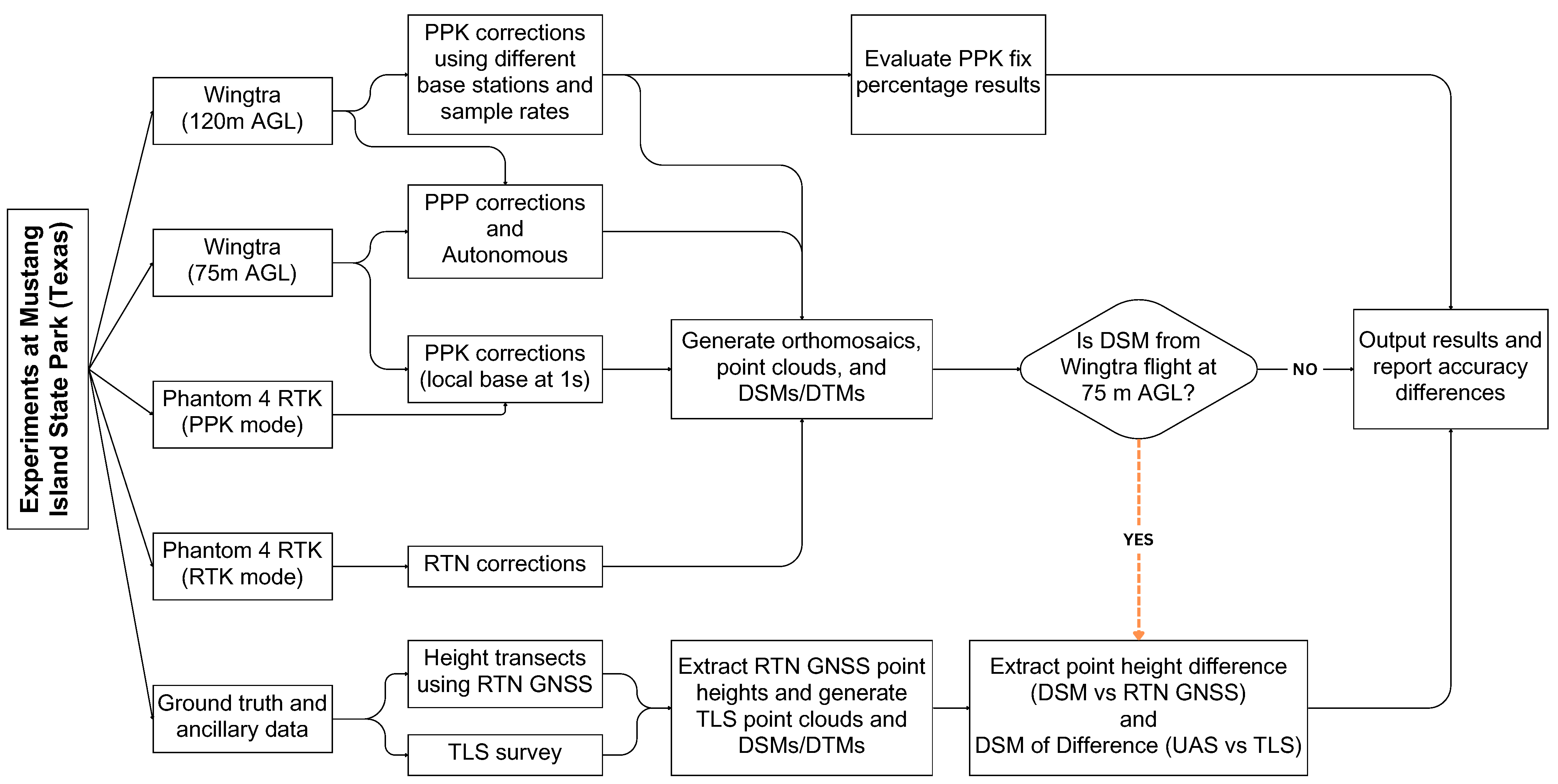
4.1. Mustang Island State Park Field Experiment

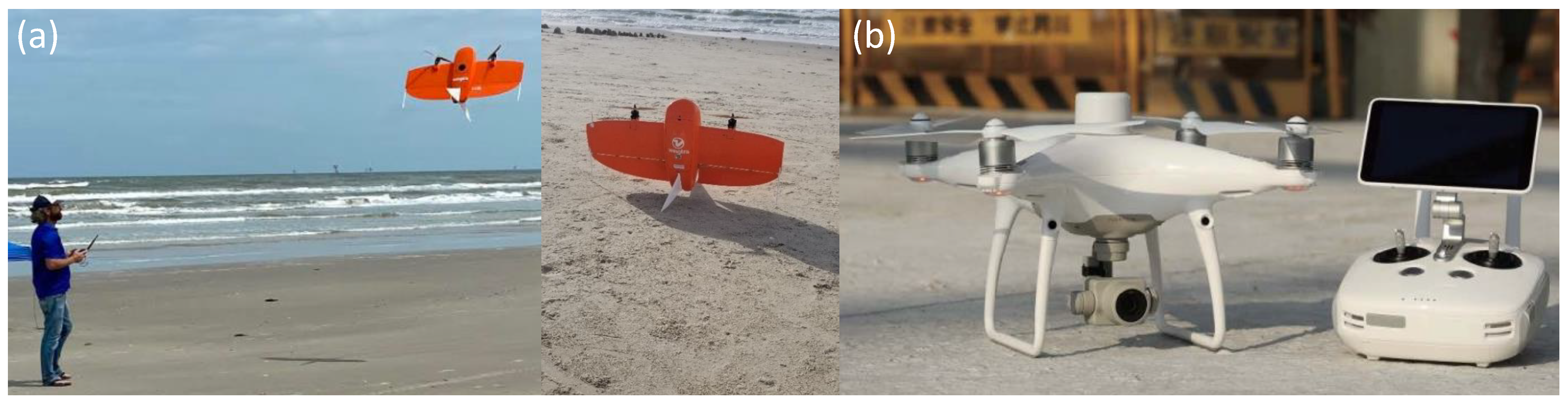
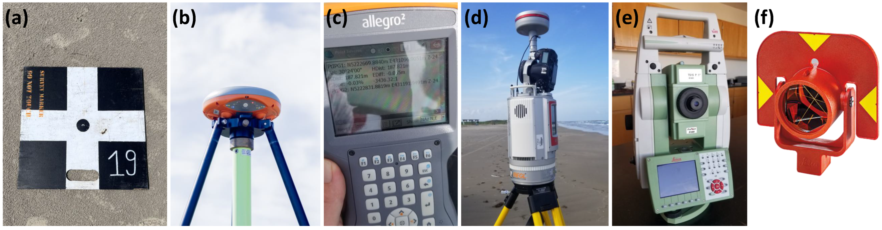
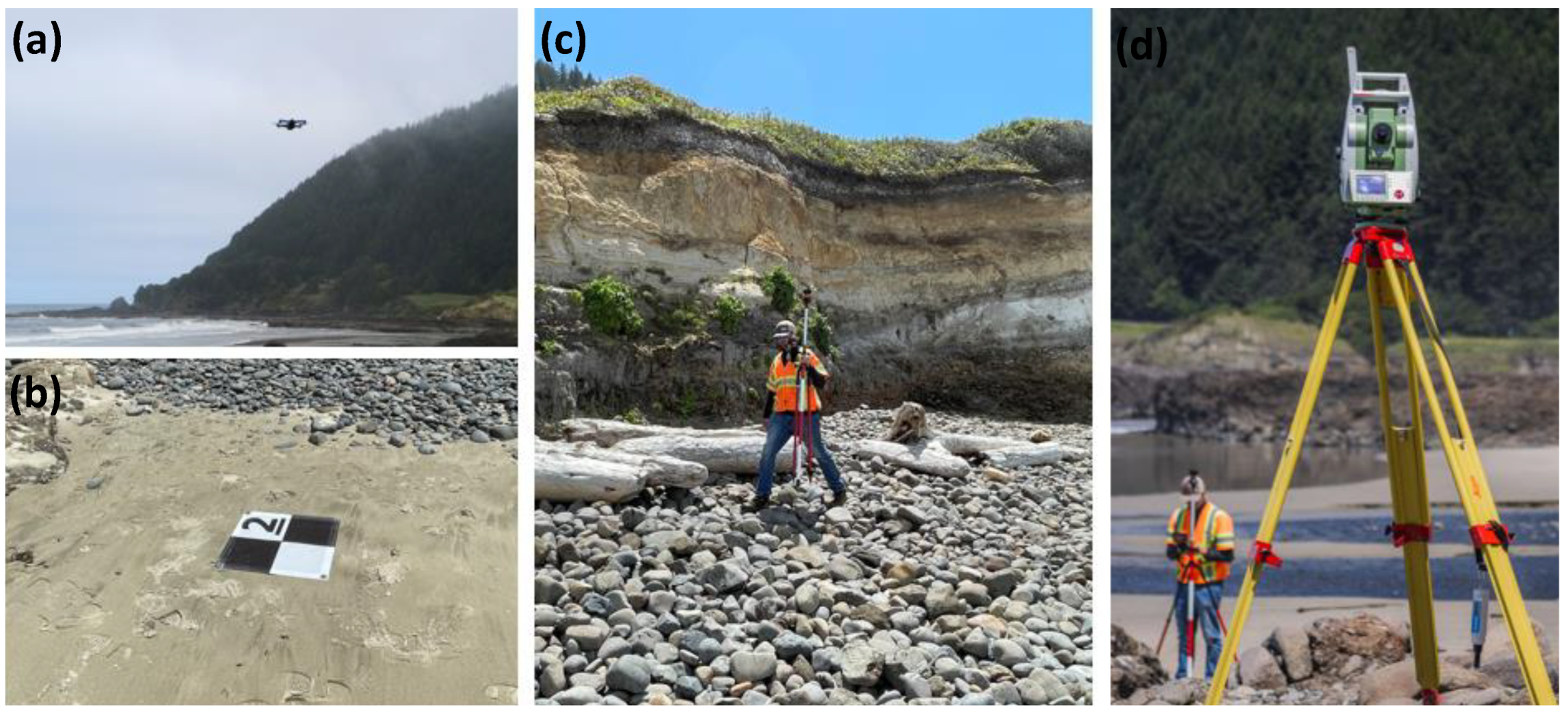
4.1.1. Hardware

This study used a WingtraOne PPK UAS (Figure 3a) and a DJI Phantom 4 RTK (Figure 3b) for image acquisition. The Wingtra is a vertical take-off and landing (VTOL) platform that has multi-frequency receiver capabilities and uses GPS and GLONASS constellations. Its sensor comprises a 42-megapixel Sony RX1 RII camera with a focal length of 35 mm [59]. The camera has a global shutter that operates at a maximum shutter speed of 1/2000 s. The Phantom 4 is a rotary system equipped with an RTK/PPK GNSS receiver [60]. Its sensor hosts an FC6310R 20-megapixel digital camera of 8.8 mm focal length. The sensor has both a mechanical and electronic shutter with maximum shutter speeds of 1/2000 s and 1/8000 s, respectively.

A series of 0.6 m × 0.6 m wooden aerial panel targets were used as checkpoints throughout the survey. An example is provided in Figure 4a. They were marked by a white cross and a dark circle in the middle. For enhanced measurement precision, white stickers were placed at the center of the dark circle. Wooden laths were used to ground all targets thus limiting their movement by water or pedestrians. GNSS data were collected using two survey-grade Septentrio NR3 GNSS receivers (Figure 4b) and an Allegro 2 data collector (Figure 4c). The GNSS receivers support multiple constellations (i.e., GPS, GLONASS, Galileo, and BeiDou), and have been described to reach RTK navigation performances within 0.6 cm + 0.5 ppm horizontally and 1 cm + 1 ppm vertically [61]. The first GNSS receiver was used for static observations at a 1-second sample rate and tied to the Texas Department of Transportation (TxDOT) RTN, via a cellular connection. The second was used as a rover receiver throughout the survey. The TxDOT RTN comprises a series of virtual reference stations (i.e., regional reference points and CORS) that facilitate real-time differential GNSS corrections. The network is made of approximately 182 reference points, 133 of which are included in the National Geodetic Survey (NGS) CORS network [62,63]. The Allegro 2 is a digital data collector that allows for both Bluetooth and Wi-Fi wireless connections, offers various stationary and non-stationary GNSS modes, and helps to track satellite information (e.g., dilution of precision and number of observable satellites) throughout the survey [64].

This study also used a Reigl VZ-2000i geodetic-grade terrestrial laser scanner (TLS) with an effective range of up to 2.5 km and a laser pulse repetition rate reaching up to 1200 kHz. The TLS operates in the near-infrared wavelength [65] and provides point colorization capabilities aided by a Nikon D810 36-megapixel camera of 20 mm focal length. In addition, the TLS has an RTK-enabled receiver, a microelectromechanical inertial measurement unit, and a compass for accurate position and orientation estimates. The TLS is shown in Figure 4d. Finally, a TS15 P 1″ robotic total station (Figure 4e) was used in combination with a Leica GPR111 circular prism (Figure 4f) to provide additional checkpoint measurements. The total station has a wavelength of 658 nm, a pulse duration of 800 ps, a pulse repetition frequency ranging from 100 MHz to 150 MHz, and a nominal ocular hazard distance of 44 m [66]. The GPR111 prism has a centering accuracy of 2 mm and a range of 2500 m [67] and it can be automatically tracked by the robotic total station. All processing was executed on a 64-bit Windows 10 computer, Intel(R) Core i7-6970 CPU at 3.00 GHz, 64 GB RAM.

4.1.2. Software

The Wingtra and Phantom 4 were operated with WingtraPilot (v1.0.0) and GS RTK (v2.2.4) applications, respectively. Carlson SurvNET (v7.0) was used for least-squares adjustments of redundant checkpoint observations acquired with the total station. Septentrio Binary Format (SBF) Converter (v21.0.0) was used to convert raw GNSS data into observation and navigation files (i.e., GPS and GLONASS). This conversion was necessary because the raw GNSS data is typically stored in binary format, which is incompatible with most GNSS processing software. Therefore, an intermediary tool was required to transform the binary data into the Receiver Independent Exchange (RINEX) format. NOAA’s Comprehensive Large Array-Data Stewardship System (CLASS, v8.2.4) service was used to download 1 s observation files for remote base stations. TEQC (Finis version of 9 February 2019) was used to decimate observation files from 1 s to 5 s, 15 s, and 30 s. The Online Positioning User Service (OPUS) was used to obtain precise base station coordinates. WingtraHub (v2.2.0) and REDtoolbox (v2.82) were used to generate PPK-corrected image geotags for the Wingtra and Phantom 4 imagery, respectively. Inertial Explorer (v8.80) was used to generate PPP-corrected image geotags for Wingtra imagery. SfM processing was performed using Pix4Dmapper (v4.6.4). Raw TLS data was processed in RiSCAN Pro (v2.12). Point cloud visualization was performed using CloudCompare (v2.10.2). LAStools (v210720) by rapidlasso was used for point cloud accuracy evaluation and generation of supplementary DEMs. Final maps were created in ArcGIS Pro (v2.9.0).

4.1.3. UAS Flight Designs

Table 1. Summary of UAS flight plans.

Platform	Wingtra	Wingtra	Phantom 4	Phantom 4
Flight mode	PPK #1	PPK #2	RTN	PPK
Number of photos	271	120	610	610
Flying height AGL (m)	75	120	59	59
GSD (cm/px)	1.0	1.6	1.6	1.6
Flight	80% sidelap	80% sidelap	Double	Double
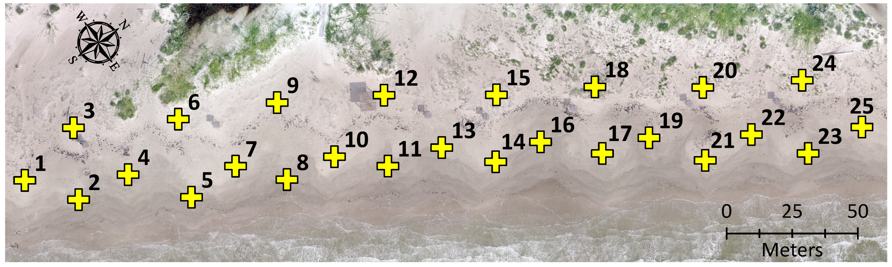
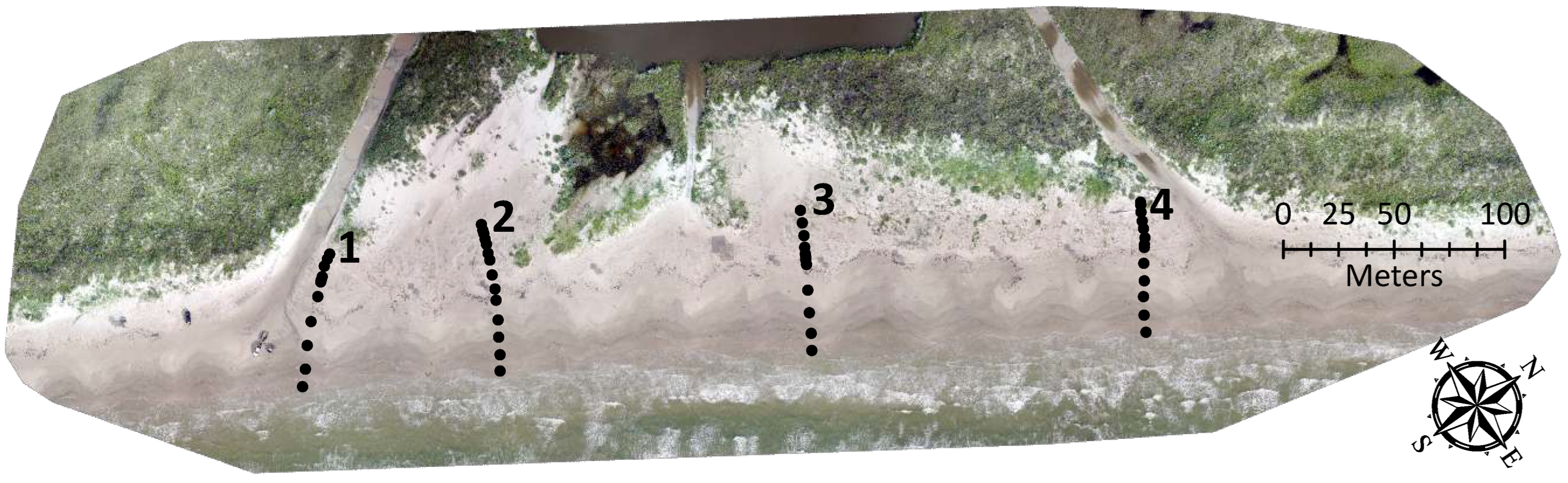
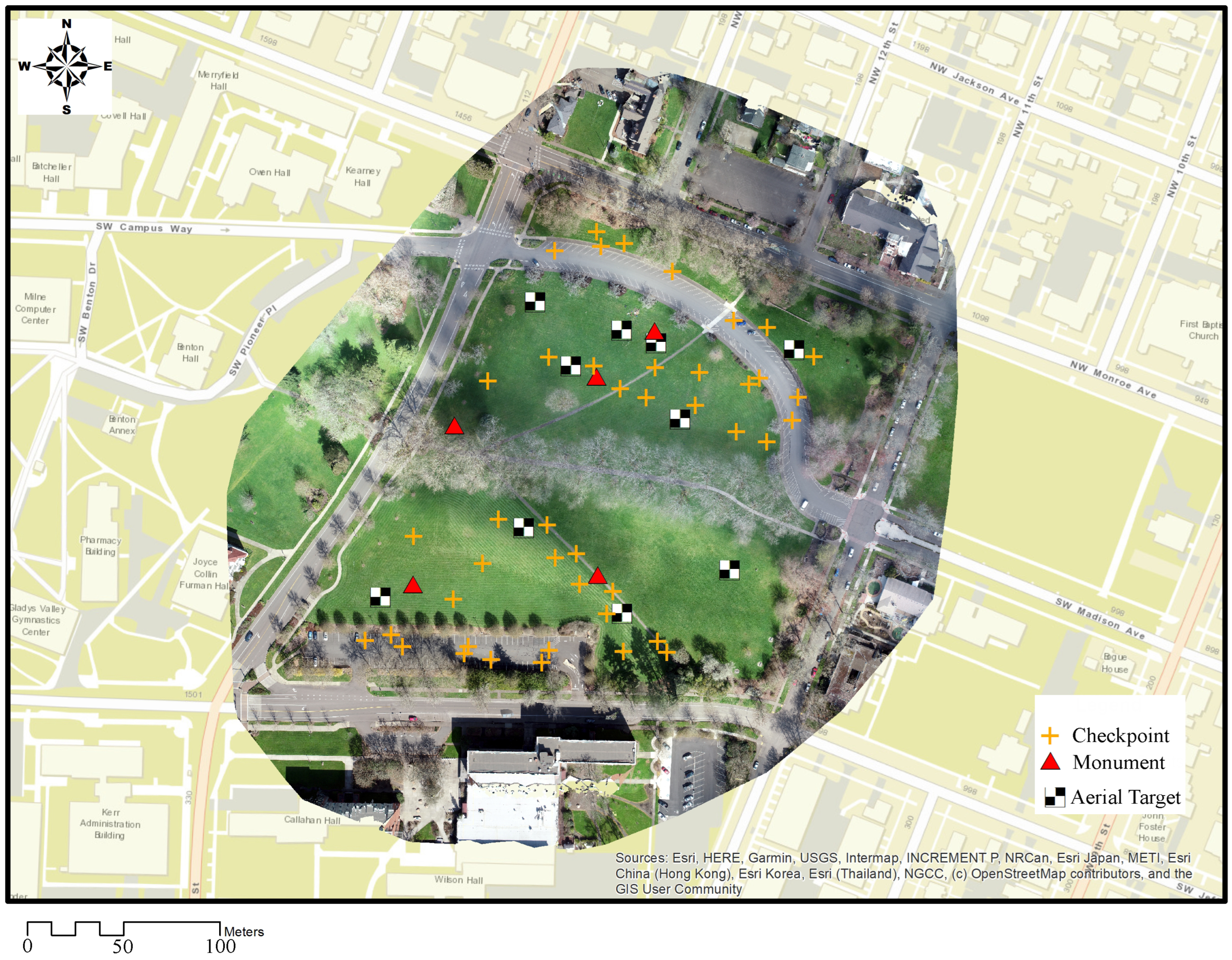
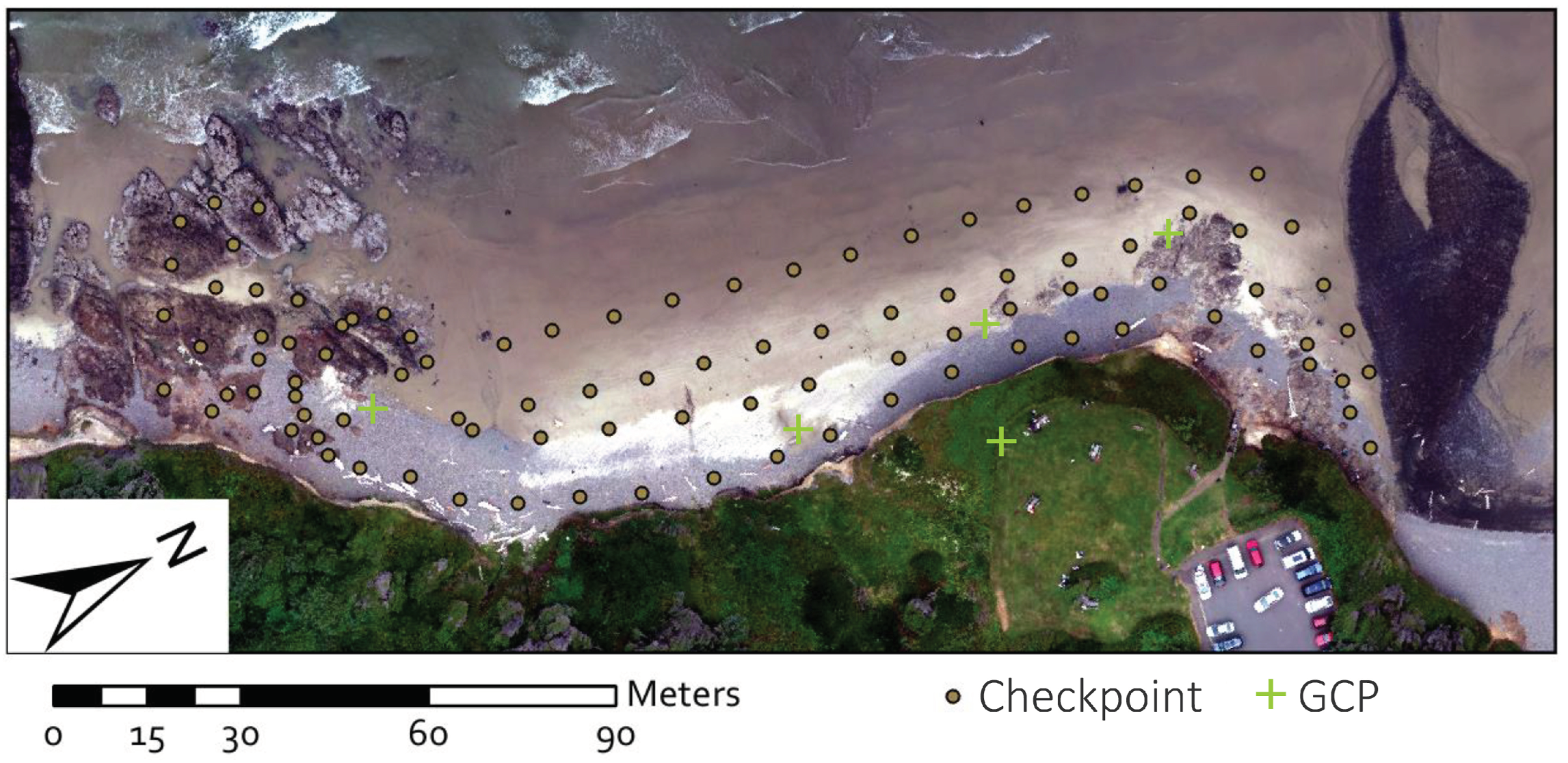
design	70% endlap	70% endlap	grid	grid

summarizes the flight designs for the Mustang Island State Park survey. The Wingtra was first flown at 75 m above ground level (AGL) and then at 120 m AGL. The lower altitude Wingtra flight yielded 271 images at 1 cm/px GSD, and the higher altitude Wingtra flight yielded 120 images at 1.6 cm/px. Both Wingtra flights were designed with 80% sidelap and 70% endlap. The Phantom 4 was first flown in RTN mode and then in PPK mode, both at 59 m AGL and using a double-grid flight design. The double-grid flight designs consist of two orthogonal flight paths, each with a sidelap of 80% and an endlap of 75%. However, the effective overlap percentage increased because new perspectives were provided through the double-grid pattern that were not present in the individual flights. Each double-gridded Phantom 4 flight resulted in a total of 610 images with a GSD of 1.6 cm/px. The RTN flight was conducted by connecting to the TxDOT RTN, which allowed RTN-corrected imagery to be generated on-site. To minimize the adverse consequences of environmental conditions on UAS-SfM products, the research team observed weather forecasts for two to three weeks ahead of the survey mission and selected a day with expected low wind speeds and no rain. The UAS flights were conducted free of rain and the maximum wind speed recorded was 3.35 m/s, which was well below the supported wind resistance of the Wingtra and the Phantom 4 (i.e., 10 m/s and 12 m/s, respectively).

4.1.4. Ground Truth

A Septentrio NR3 GNSS receiver was used for a six-hour static survey at a logging rate of 1 s. This survey was conducted to establish the local base station for PPK corrections of UAS trajectories. For accurate results, Trimble GNSS Planning was used to anticipate satellite observability and geometry on the day of the survey. Twenty-five checkpoints (Figure 5) were distributed throughout the site and used for accuracy validation.

The checkpoints were spaced 20 m apart and surveyed using both RTN GNSS and a total station. RTN GNSS observations of the checkpoints were also aided by the TxDOT RTN, each consisting of a 10-second average. The total station measurements used a resection technique in which each checkpoint was observed from two pre-established locations and later corrected using a least-squares adjustment. These two locations were marked by survey rebars and their coordinates were determined via the same RTN GNSS approach applied for checkpoint measurements. After the least-squares adjustment, the RMSE between the RTN GNSS and the total station observations was 1.65 cm.

In addition, four cross-shore transect measurements spaced approximately 100 m apart were obtained using RTN GNSS to validate the accuracy of the DSMs generated using UAS-SfM. The transects are depicted in Figure 6. For each transect, the measurements started near the wet/dry shoreline and were carried until the foredune. The number of points collected for each transect ranged between eleven and fourteen, depending on the distance between the shoreline and the foredune.

Finally, the Reigl V-2000i TLS was used to create point cloud data, which in turn was used to generate a DSM that allowed a comparison against the Wingtra-generated DSM. The TLS was deployed from three set-up positions at a stepping angle of 20 millidegrees and its horizontal and vertical fields of view were 360° and 70° (+30°, −40°), respectively. A multi-station adjustment report was generated during post-processing that provided additional information about the TLS scan. Specifically, the number of points collected was reported to be 108,385,456, acquired with 3D accuracies within 0.015. These accuracies represent the expected GNSS measurement error in the horizontal and vertical directions.

The geometric datum for the project was set to the North American Datum of 1983 (NAD 83), epoch 2010.0. Coordinates were projected in the State Plane Coordinate System of 1983 (SPCS83), Texas South Zone.

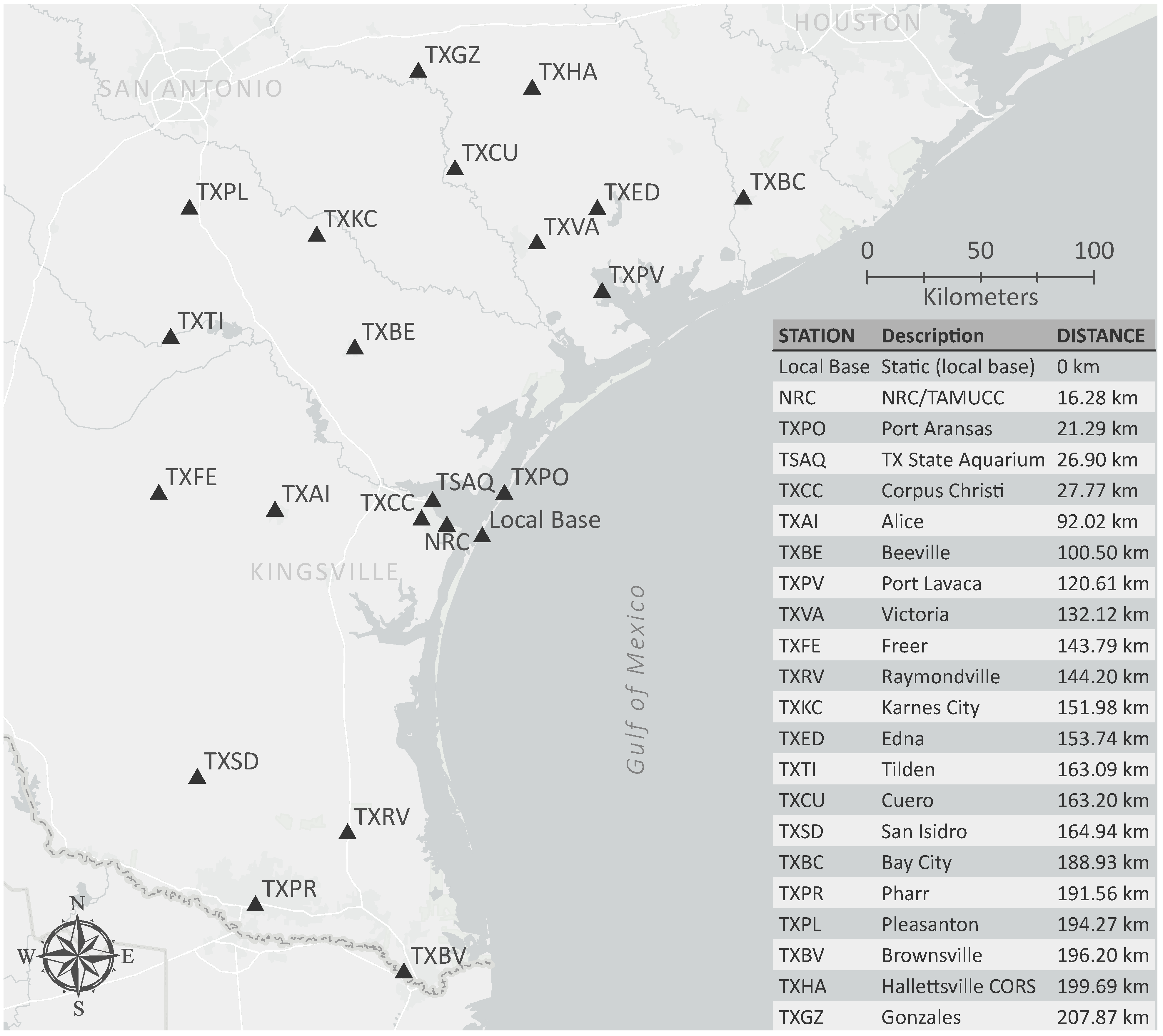
4.1.5. Data Processing and GNSS Evaluation

This study considered NOAA’s vertical error budget requirements (i.e., 0.5 m vertical accuracies are required when surveying exposed land surfaces and submerged areas to depths of 100 m at the 95% confidence level [57]) for evaluating the different GNSS techniques. The tests performed with these datasets are summarized as follows:

• Test 1: UAS-SfM vertical accuracy assessment when using RTN GNSS to correct the location of Phantom 4 imagery (flown in RTK mode).
• Test 2: Examination of UAS-SfM vertical accuracies when using PPK GNSS to correct the location of images from the Phantom 4 (flown in PPK mode) and the two Wingtra flights (i.e., 75 m AGL and 120 m AGL).
• Test 2.1: Influence of PPK base station distance on UAS-SfM vertical accuracy, using imagery from the Wingtra at 120 m AGL.
• Test 2.2: Effects of different GNSS sample rates on PPK corrections (i.e., 1 s, 5 s, 15 s, and 30 s), using imagery from the Wingtra at 120 m AGL.
• Test 2.3: Influence of the PPK fix percentage on the accuracy of UAS-SfM mapping products, using imagery from the Wingtra at 120 m AGL.
• Test 3: Assessment of UAS-SfM vertical accuracies when using PPP GNSS to correct image geotags, using imagery from the two Wingtra flights.
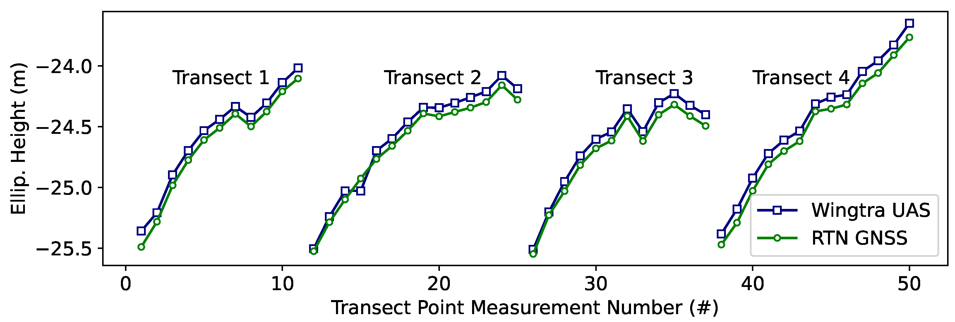
• Test 4: Comparison between UAS-SfM-derived DSMs (using the Wingtra-generated DSM at 75 m AGL) and point heights extracted from cross-shore transects measured using RTN GNSS.
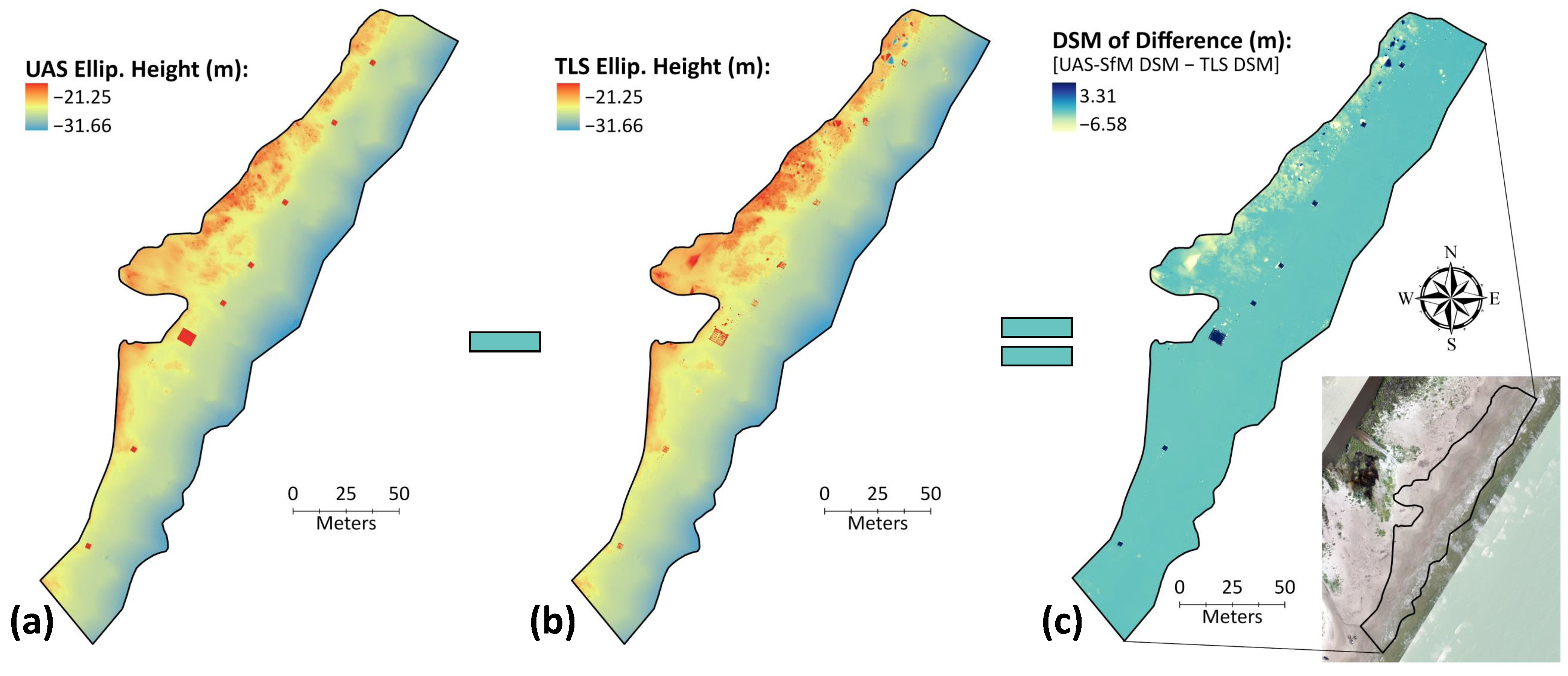
• Test 5: Comparison between DSMs generated using UAS-SfM (i.e., Wingtra at 75 m AGL) versus DSMs generated using the geodetic-grade Reigl VZ-2000i TLS.
• Test 6: Supplementary processing of Wingtra data without additional corrections of image geotags for comparison against RTN, PPK, and PPP GNSS.

Figure 7 summarizes the workflow used for the GNSS assessments conducted in this portion of the study.

To conduct the RTN GNSS experiment with the Phantom 4 (flown RTK mode), the UAS was tied to the TxDOT RTN via an Internet Protocol connection using an AT&T SIM card. Because RTN offers real-time solutions, no additional GNSS processing was needed after the survey and the images were ready for processing in Pix4Dmapper. In this case, the RTN-corrected image coordinates were embedded in the exchangeable image file format (EXIF) property of the images.

As mentioned earlier, the PPK GNSS evaluation used imagery from the Phantom 4 (flown in PPK mode) and the two Wingtra flights (75 m AGL and 120 m AGL). PPK corrections for the Wingtra imagery were performed using WingtraHub, while REDtoolbox was used for correcting Phantom 4 imagery. Wingtra imagery was further processed using various base stations and sample rates whereas Phantom 4 Pro images were corrected relative to the local base station at a 1 s sample rate. Corrected image coordinates from WingtraHub were exported to a separate comma-separated values (CSV) file. Corrected image coordinates from REDtoolbox were embedded in the imagery EXIF data. PPK corrections required observation and navigation files corresponding to the relevant base station. When using the local base, observation and navigation files were generated from the raw GNSS data using SBF Converter. In addition to the local base established via a static GNSS observation, there were twenty-one other base stations (i.e., the remote base stations), illustrated in Figure 8.

When using remote base stations, observation and navigation files were downloaded from CLASS and GNSS servers maintained by Texas A&M University–Corpus Christi and Louisiana State University servers. CLASS is a free service that stores original CORS data. While CORS data are typically accessible through the NGS User Friendly CORS (UFCORS) online service, UFCORS generally decimates data to a 30-second sample rate after one month. Thus, CLASS is a plausible source for original CORS data should a user require undecimated GNSS data beyond this period. The university servers provided GNSS data for the NRC and TSAQ stations, which are not available through CLASS. Wingtra imagery was also used to examine the impact of baseline distance, observation rate, and PPK fix percentage on vertical accuracies. The effects of baseline distance were evaluated using the various base stations described above. The observation rate was examined by decimating the 1-second GNSS data into 5 s, 15 s, and 30 s. Lastly, the PPK fix percentages were obtained from the WingtraHub processing report after the correction of UAS image locations.

The PPP GNSS evaluation used both sets of Wingtra imagery. Unlike PPP services such as RTKLIB, Inertial Explorer supports raw GNSS data and does not require converting the raw GNSS data into RINEX format before further processing. Although the converted files can also be used, importing the raw GNSS file directly saves processing time and reduces blunders. Moreover, the raw GNSS file holds encoded camera event information which Inertial Explorer can decode and use during PPP processing. PPP uses only GNSS data from the rover receiver; therefore, no information about a base station is needed. In this study, the multi-pass processing direction was adopted, which combines forward and reserve passes, and helps to minimize the impact of GNSS errors on PPP corrections.

The SfM processing pipeline in Pix4Dmapper consisted of first importing the UAS imagery and respective image geotags. This included multiple instances of image locations (i.e., geotags) corrected using the various GNSS techniques that were investigated (i.e., RTN, PPK, or PPP) as well as using autonomous GNSS (uncorrected image locations). During the bundle block adjustment, keypoints in overlapping images were extracted using the original image scale, and image pairs were matched based on the aerial grid or corridor method. At this stage, the standard calibration method in Pix4Dmapper was used, which is a self-calibration process whereby internal and external camera parameters are determined, and all photos are aligned to a uniform coordinate system. The internal calibration accounts for parameters such as focal length, optical center, and lens distortion coefficients (i.e., radial and tangential). The external calibration accounts for the position and orientation of the UAS camera sensor. Once the initial bundle block adjustment had taken place, the checkpoints (i.e., aerial panel targets) were imported and tagged during the analysis for accuracy validation purposes. These checkpoints were used to estimate coordinate solutions and model reprojection errors without altering or constraining the model to the coordinates of the checkpoints. Next, densification was performed at a half-image scale and the resulting point cloud was classified to allow for DSM and DTM generation. DSMs were exported with a 5 cm spatial resolution, using the inverse distance weighting method. DTMs were also exported at 5 cm spatial resolution, aided by the classified point cloud that allowed for filtering out non-terrain features. Orthomosaics were exported at the highest possible spatial resolution. The exact resolution of orthomosaics varied depending on the UAS image GSD, which is dictated by factors such as sensor characteristics, overlap between the UAS images, and the flying height of the UAS platform.

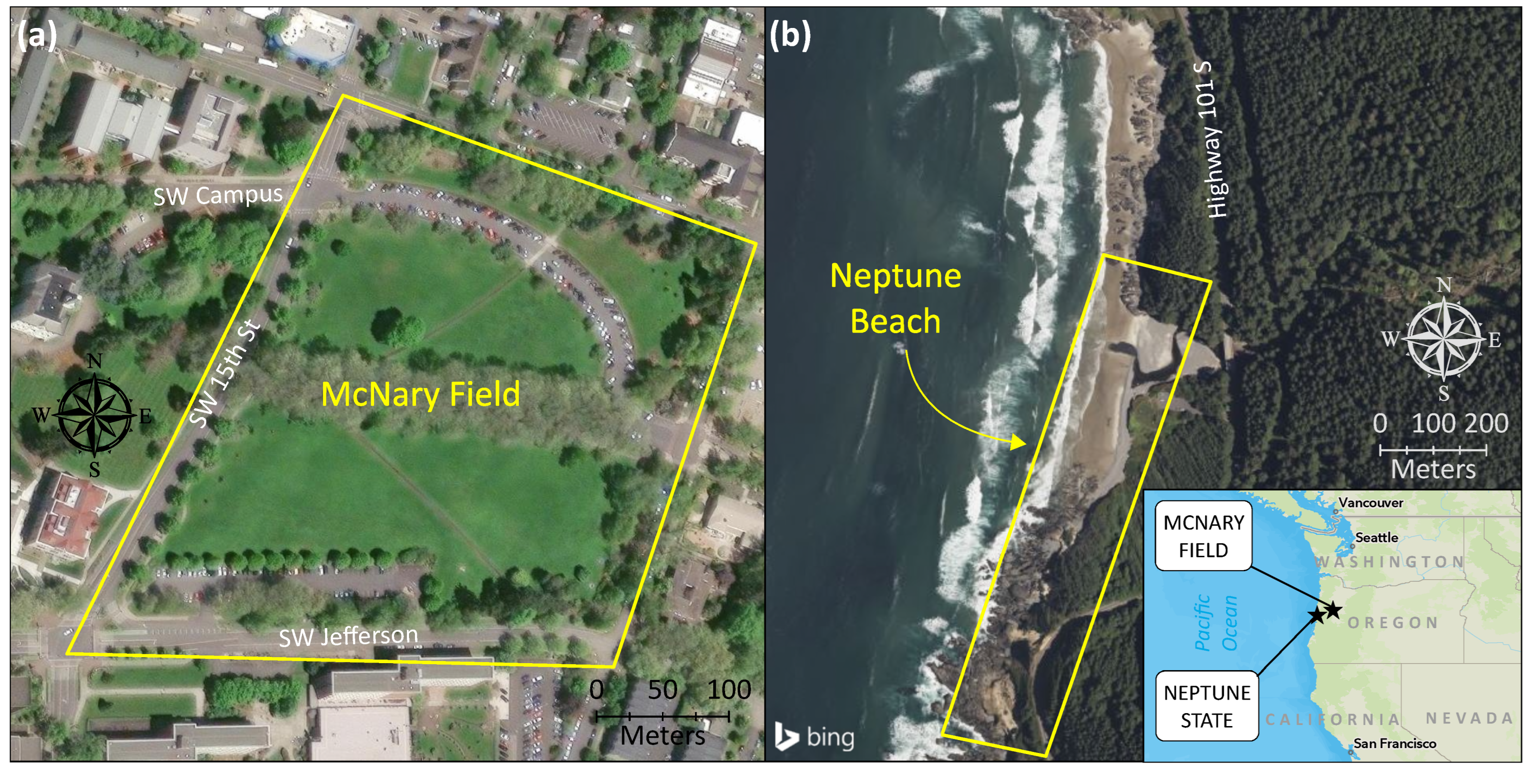
4.2. McNary Field and Neptune State Scenic Area Field Experiments

4.2.1. Hardware

At the McNary Field and Neptune State Scenic Area study sites, UAS data collection was also conducted using a Phantom 4 RTK UAS. The specifications of this platform were previously detailed in Section 4.1.1. In addition, a series of 0.6 m × 0.6 m center eyelet aerial targets were deployed as GCPs. The center eyelet enabled the placement of survey nails through the center of the target, which allows for accurate survey measurements. These targets featured a black-and-white checkerboard pattern. Ground data collection was supplemented by a Leica TS15P 1″ total station, paired with a Leica 360° prism for checkpoints and a circular prism for control points. Additionally, a Leica GS14 GNSS receiver and a 2-meter fixed-height survey rod with bipod legs were used. The different hardware equipment used in these study sites is shown in Figure 9.

4.2.2. Software

MicroSurvey STAR*NET Pro was used for a least-squares adjustment of GCP survey. RTKLIB was used for PPK correction of UAS imagery. The simulation environment was built upon Blender, as outlined in [55]. It is supported by code and functionalities of MATLAB, Python, and Agisoft Metashape. Leica Infinity was used to compute the baselines between the base station and GCPs. SfM processing was performed in Agisoft Metashape.

4.2.3. UAS Flight Designs

At McNary Field, the Phantom 4 was flown at 100 m AGL using an overlap (i.e., endlap and sidelap) of 75%. This was selected to remain consistent with the parameter settings used in the simulation portion of this study. A total of eight flight lines were conducted, resulting in 74 images with a GSD of 2.74 cm/px. At the Neptune State Scenic Area, the Phantom 4 was deployed 73 m AGL, also using an overlap of 75%. The resulting photos were captured with a GSD of 2 cm/px. In these study sites, the UAS platforms were also deployed on days of calm wind conditions.

4.2.4. Ground Truth

Similar to the first experiment, the field experiments at McNary Field and Neptune State Scenic Area also measured double angles (i.e., direct and reverse) on GCPs to enable resection and a least-squares adjustment of results. A topo shoe was used in the survey rod for the checkpoints, due to the soft ground surface. The circular prisms were mounted on tribrachs with adjustable-leg tripods to ensure precise centering over the control points, while the 360° prism was mounted on the survey rod, supported by bipod legs, facilitating direct and reverse mode readings at the checkpoints. In addition, a static GNSS receiver was deployed on-site for approximately four hours, which served as the basis for obtaining precise base station coordinates for subsequent PPK correction. Figure 10 illustrates the distribution of control points and checkpoints at McNary Field, which included five existing monuments, ten GCPs, and forty-three checkpoints. The existing monuments, comprising benchmarks and survey rebars located at the site, were used as instrument (i.e., total station) and backsight stations when conducting the double-angle GCP survey used for resection. The aerial targets correspond to the center eyelet aerial targets of checkerboard pattern (Figure 9b) that were used as GCPs during SfM processing of UAS imagery. Finally, the checkpoints were used to validate the accuracy of UAS-SfM results.

Figure 11 depicts the GCP and checkpoint distribution at Neptune State Scenic Area, consisting of five GCPs and ninety-seven checkpoints. The GCPs also consisted of center eyelet aerial targets (Figure 9b) while the checkpoints consisted of GNSS measurements acquired throughout the survey area. This included shots of rocky, grassy, and paved features, all of which were also used to validate the accuracy of the resulting UAS-SfM accuracies. The surveys were referenced to the Oregon North Zone of NAD83 (2011), epoch of 2010.00, orthometric heights relative to the NAVD88 datum using GEOID18.

4.2.5. Data Processing and GNSS Analyses

When correcting Phantom 4 imagery with PPK GNSS, the procedure for the McNary Field and Neptune State Scenic Area datasets followed the same approach used in the Mustang Island State Park experiment. Raw GNSS data were processed to obtain observation and navigation files, which were then used for PPK correction of the imagery. The least-squares adjustment of GCP measurements was performed using MicroSurvey STAR*NET Pro. Precise coordinates for the locally established base stations were acquired by submitting the observation file to OPUS. Unlike the Mustang Island State Park experiment, these last two surveys did not consider remote base stations. The vertical accuracy assessment considered both the point cloud and the GNSS components. Accuracy tests were performed according to the first edition of the American Society for Photogrammetry and Remote Sensing (ASPRS) Positional Accuracy Standards for Digital Geospatial Data [68]. Once PPK corrected, UAS imagery was imported into Metashape for SfM processing and generation of 3D point clouds. The SfM processing workflow followed the Metashape documentation for processing coastal imagery [69], which started with importing the UAS imagery and PPK-corrected image locations (or geotags) into the processing pipeline for image alignment and the bundle block adjustment. This step also included a self-calibration mechanism whereby the interior and exterior camera parameters were refined [70]. This also accounts for internal camera parameters such as focal length, optical center, distortion coefficients, and external parameters such as position and orientation of the UAS camera. Alignment was performed using the high-accuracy setting. The keypoint and tie point limits were set to 60,000 and 4000, respectively. In these two study sites, GCPs (i.e., eyelet center targets) were introduced to further refine the bundle block adjustment and constrain the derived model to the coordinates of the GCPs. The adjustment was optimized using the workflow outlined in the Metashape workflow documentation. A series of independently surveyed checkpoints (natural ground shots) were tagged during the analysis for accuracy validation. Next, point cloud densification was performed using the high-quality setting, and mild-depth filtering, and both point clouds and point confidence values were calculated. The resulting point cloud was then used for all assessments performed at the McNary Field and the Neptune State Scenic Area.

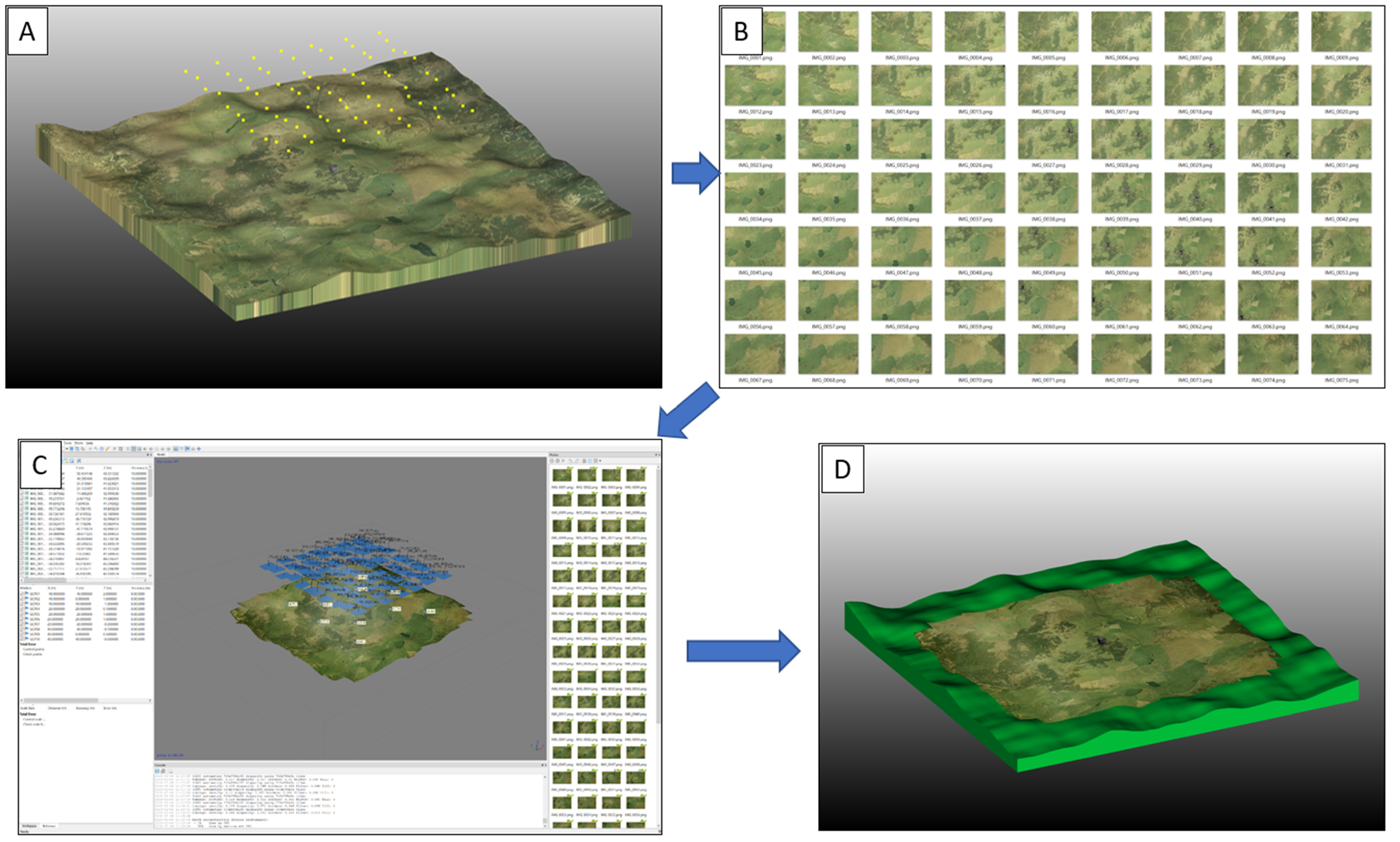
4.3. Simulated Tests (simUAS)

The simulation implemented herein followed a previous workflow discussed in [55]. The authors developed an ecosystem called simUAS using Blender, custom MATLAB and Python codes, and Agisoft Metashape software. simUAS consists of generating photo-realistic images of simulated scenes in a similar manner to UAS-acquired images. The images are then processed in SfM software to generate orthomosaics and point clouds. simUAS allows users to test the influence of different parameters that affect UAS-SfM mapping, such as flight path, flying height AGL, and camera focal length. The simUAS environment allows for conducting accuracy tests in environments where only one variable is changed at a time. In addition, it eliminates uncontrollable variables that affect UAS-SfM mapping such as illumination and moving objects at the scene being mapped.

Figure 12 summarizes the general workflow with simUAS. First, the terrain model and texture of the simulated scene are generated and lighting is added to achieve the desired level and type of illumination. Next, camera stations with the associated overlap are created. Then, the simulated block of UAS imagery for the scene is generated and lens distortion, vignetting, noise, and blur are added to the imagery using the custom MATLAB code. Next, SfM software is used to create the desired geospatial products (i.e., orthomosaics and point clouds). Finally, accuracy assessments are conducted by comparing the coordinates of points in the point cloud versus those from the simulated scene.

In this experiment, simUAS was used to create a 9 × 9 photogrammetric block of images with a 75% overlap (i.e., endlap and sidelap). Other simulated parameters include a flying height AGL of 100 m, a Sony A6000 digital camera (24 megapixels), a 30 mm focal length, and a GSD of 1.3 cm/px. The effects of GNSS accuracy on the SfM point cloud were examined by successively degrading the camera positions by adding increasing amounts of Gaussian noise. A total of nine different quality levels were simulated and, for each, fifteen Monte Carlo trials or iterations were performed. The Monte Carlo analysis also provided uncertainty estimates based on the spread of the output of the fifteen realizations.

4.4. Accuracy Evaluation and SfM Processing

Accuracy assessments were based on RMSE_z values retrieved from SfM processing reports. All RMSE_z values are reported relative to independently surveyed checkpoints. Tables and plots were used to compare and visualize performance and accuracy differences across the various georeferencing methods. Additional tests (i) compared the differences in accuracies of RTN GNSS surveyed checkpoints versus using a total station, (ii) evaluated the difference between a UAS-generated DSM versus that of a TLS, and (iii) quantified height differences between the Wingtra UAS and RTN GNSS at selected locations.

5. Results

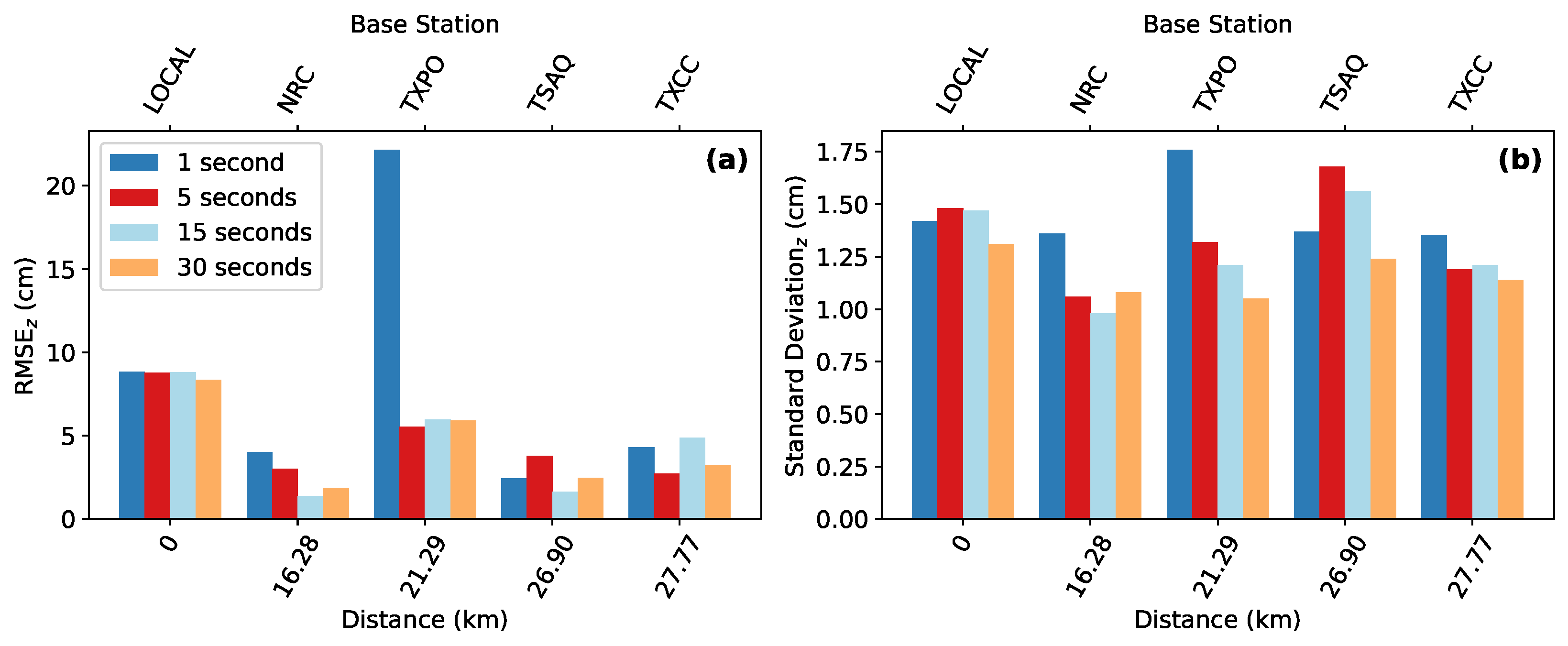
5.1. GNSS Evaluation Results—Mustang Island State Park

The RTN GNSS experiment resulted in an RMSE_z of 7.27 cm. The PPK GNSS evaluation results using the Wingtra UAS are threefold: baseline distance, sample rate, and the effects of the PPK fix percentage. The RMSE_z values of the UAS-SfM solutions relative to checkpoints are shown in Figure 13a. Note that stations within 30 km produced errors not exceeding 6 cm (except for the local base and the 1 s instance at TXPO). For example, at 30 s, the resulting RMSE_z values for NRC, TXPO, TSAQ, and TXCC were 1.87 cm, 5.92 cm, 2.47 cm, and 3.21 cm, respectively. Figure 13b shows the standard deviation of the checkpoint measurements; it suggests precision decreased as the baseline distance increased. Figure 14 shows these observations exclusively for stations located within 30 km of the survey site.

Figure 15 shows the relationship between RMSE_z and baseline distances at 5 s and 30 s, using linear, polynomial, and exponential fits. At 5 s, with the local base included, the R² values for the linear, polynomial, and exponential fits were 0.649, 0.715, and 0.717, respectively. Without the local base, these values were 0.653, 0.708, and 0.707. At 30 s, with the local base included, the R² values were 0.509, 0.628, and 0.633, and, without the local base, they were 0.520, 0.620, and 0.626.

Overall, results from the sample rate experiment observed the lowest average RMSE_z values and pertinent standard deviations at 5 s and 30 s sample rates.

Table 2. Statistical values for RMSE_z at different sample rates for base stations located within 30 km.

	Min (cm)	Max (cm)	Mean (cm)	Median (cm)	Sigma (cm)
1 s	2.44	22.16	8.35	4.31	7.23
5 s	2.73	8.79	4.77	3.78	2.44
15 s	1.38	8.81	4.54	4.89	2.79
30 s	1.87	8.36	4.37	3.21	2.43

provides the statistical metrics for base stations within 30 km of the study site and different sample rates. The respective mean and standard deviation of RMSE_z values were 8.35 cm and 7.23 cm at 1 s, 4.77 cm and 2.44 at 5 s, 4.54 cm and 2.79 cm at 15 s, and 4.37 cm and 2.43 at 30 s.

Table 3. Statistical values for RMSE_z at different sample rates for all stations.

	Min (cm)	Max (cm)	Mean (cm)	Median (cm)	Sigma (cm)
1 s	2.44	128.42	40.91	26.44	37.32
5 s	2.73	68.29	28.17	24.83	20.05
15 s	1.38	121.36	29.49	20.55	27.51
30 s	1.87	79.83	24.18	16.93	21.48

provides the statistical metrics for all base stations and sample rates. Here, the 5 s and 30 s sample rates consistently yielded the lowest mean RMSE_z and vertical standard deviation values compared to 1 s and 15 s. For example, the respective mean and standard deviation of RMSE_z values were 40.91 cm and 37.32 cm at 1 s, 28.17 cm and 20.05 cm at 5 s, 29.49 cm and 27.51 cm at 15 s, and 24.18 cm and 21.48 cm at 30 s. Figure 16 also illustrates these results.

The results from PPK corrections using Phantom 4 imagery yielded an RMSE_z of 8.44 cm relative to checkpoints. PPP-corrected solutions using Wingtra imagery yielded RMSE_z values of 32.86 cm at 75 m AGL and 90.80 cm at 120 m AGL. The results suggest good satellite availability and geometry throughout the survey period as the positional dilution of precision remained mostly below 1.45. This is consistent with the values obtained from the Trimble GNSS Planning service.

Recall that some assessments were conducted to compare differences in accuracies between RTN GNSS and a total station. This was accomplished using PPK solutions from the Wingtra flight at 120 m AGL. As

Table 4. Performance comparison of total station and RTN GNSS surveyed ground control.

Survey Mode	PPK Sample Rate (s)	Mean (cm)	Sigma (cm)	RMSEz (cm)
Total station	1	−8.74	1.42	8.85
RTN GNSS	1	−8.32	2.42	8.66
Total station	30	−8.26	1.31	8.36
RTN GNSS	30	−7.84	2.27	8.16

shows, the resulting differences in RMSE_z values between the two methods were within subcentimeters (i.e., 1.9 mm to 2 mm, depending on the sample rate used), with the total station measurements carrying the lower RMSE_z values. Specifically, the RMSE_z values for the total station measurements were 8.85 cm at the 1 s sample rate and 8.36 cm at 30 s. Likewise, the RMSEs for the RTN GNSS-surveyed checkpoints were 8.66 cm and 8.16 cm at 1 s and 30 s, respectively.

Next, the study compared the differences in DSMs generated from the Wingtra flight at 75 m AGL and the TLS. The computation and resulting differences are illustrated in Figure 17. The difference in heights ranged from −6.58 m to 3.31 m, with an RMSE of 0.16 m. However, an average height of 8 mm suggests that the wide range might be biased due to inherent differences in data acquisition between the two methods. This includes differences in perspective between the two systems (aerial and nadir versus terrestrial and oblique), nature of sensor deployment (i.e., UAS-SfM relies on keypoint detection and matching across multiple images for surface reconstruction while the TLS relies on active laser pulses sent to and received from features of interest), all of which affect point density and contribute to variations in surface representations, especially more complex features as illustrated in Figure 17.

Furthermore, a comparison between the heights obtained from RTN GNSS and the Wingtra-derived DSM at 75 m AGL yielded centimeter-level vertical differences between the two methods across all transects. The RMSE_z differences ranged between 0.073 m and 0.094 m. The differences between the various transects are shown in

Table 5. Mean, standard deviation, and RMSE_z of height differences between RTN GNSS and UAS.

	Transect 1	Transect 2	Transect 3	Transect 4
Mean of differences (m)	0.080	0.055	0.072	0.093
Std. dev. of differences (m)	0.018	0.047	0.021	0.014
RMSEz (m)	0.082	0.073	0.075	0.094

and Figure 18.

The performance of the various GNSS correction techniques explored in this study and whether they satisfy NOAA standards can be evaluated based on the product between the RMSE_z values from processing reports and a factor of 1.96 (the conversion factor to obtain a 95% confidence level, assuming normally distributed errors). The results are summarized in

Table 6. Summary of results for various GNSS techniques tested in this case study.

Processing Mode	Dataset	RMSEz × 1.96 (cm)	Result
RTN	Phantom 4 (RTN mode)	14.25	Pass
PPK (Local Base, 1 s)	Phantom 4 (PPK mode)	16.54	Pass
PPK (Local Base, 1 s)	WingtraOne (75 m AGL)	10.37	Pass
PPK (Local Base, 1 s)	Wingtra (120 m AGL)	17.35	Pass
PPP	Wingtra (75 m AGL)	64.41	Fail
PPP	Wingtra (120 m AGL)	177.97	Fail
Autonomous	Wingtra (75 m AGL)	1864.76	Fail
Autonomous	Wingtra (120 m AGL)	3070.38	Fail

and consist of the following: 14.25 cm for RTN; 10.37 cm, 16.54 cm, and 17.35 cm for different PPK instances at the local base; 64.41 cm and 1.77 m for PPP at different heights; and 18.64 m and 30.70 m for uncorrected/autonomous flights. These are influenced by different platforms and/or altitudes flown.

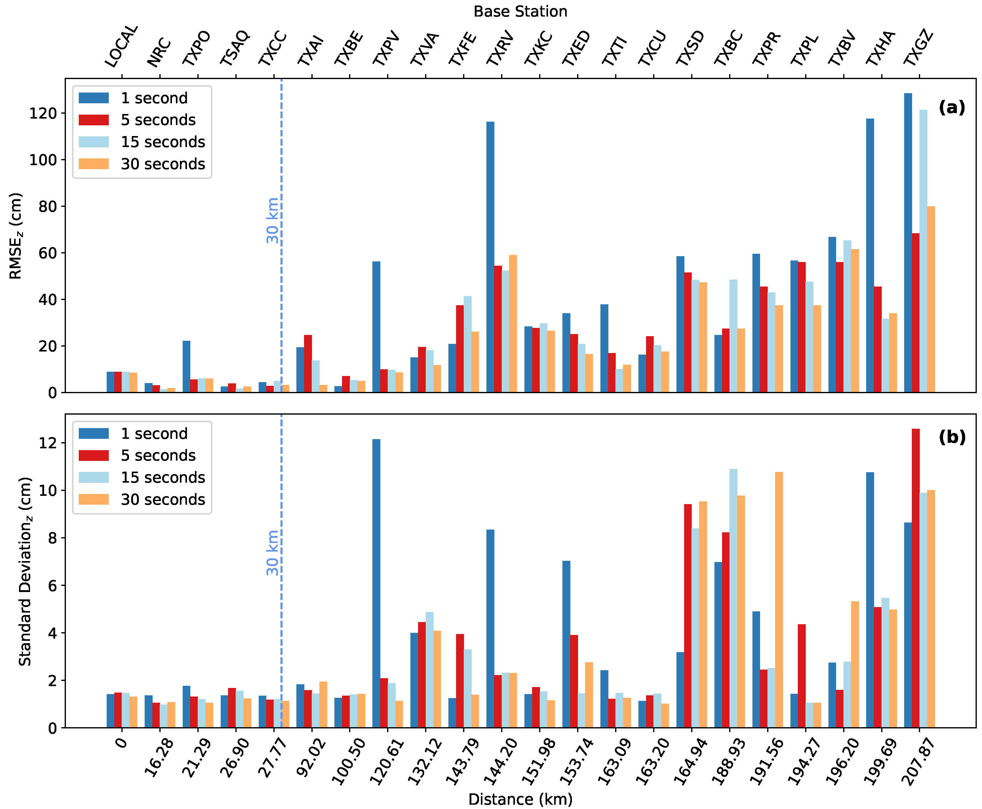
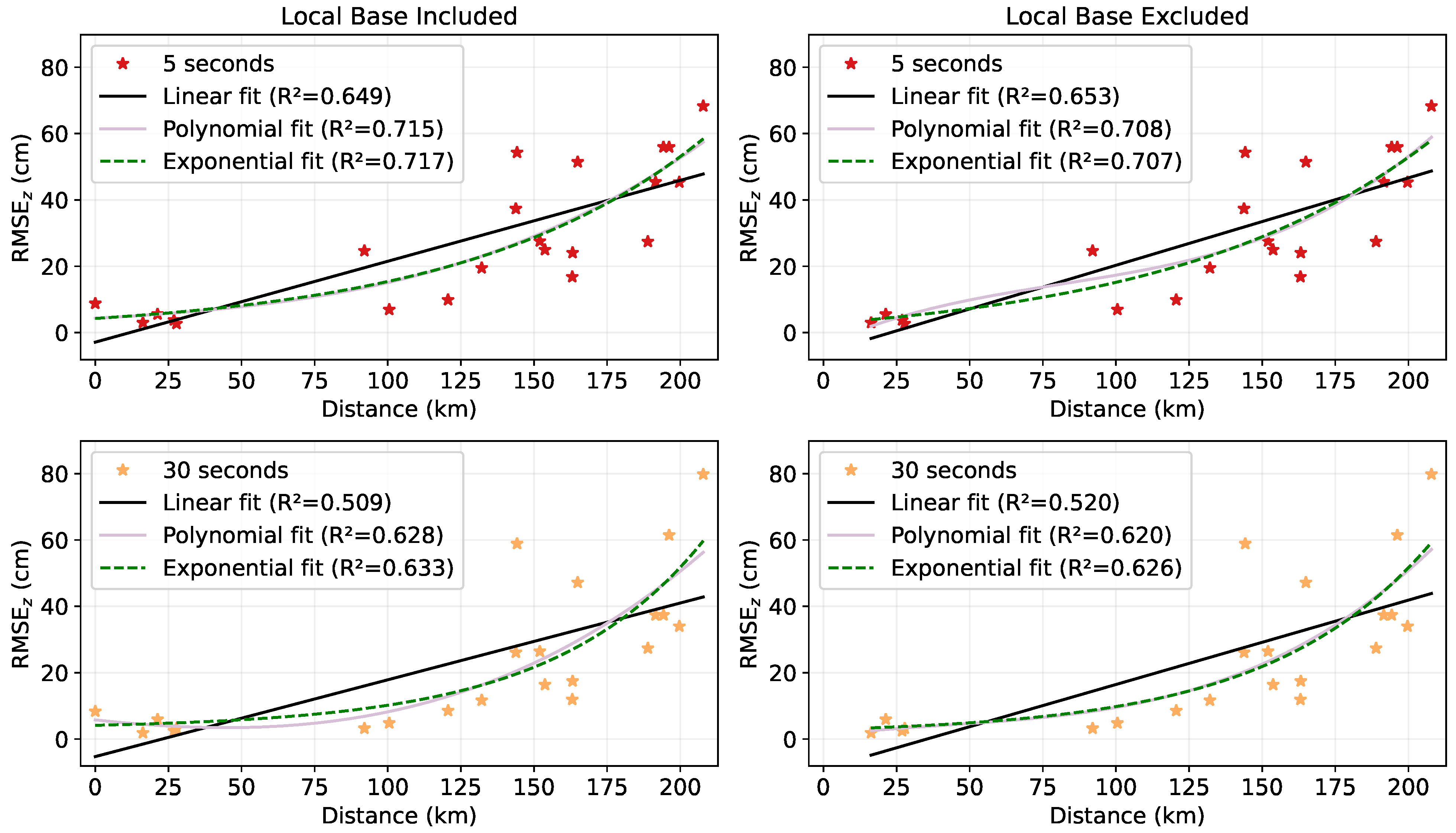
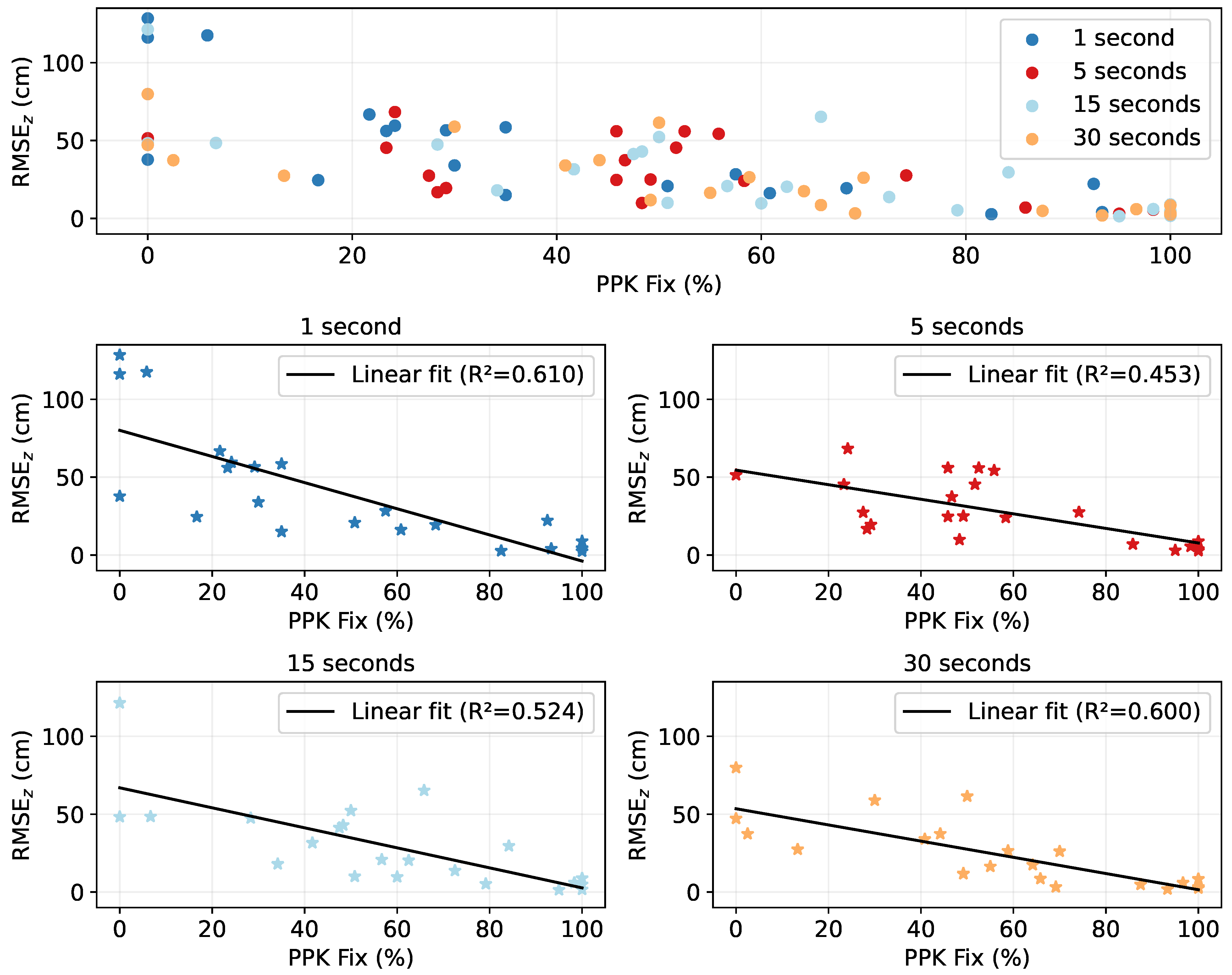
5.2. GNSS Evaluation Results—McNary Field and Neptune State Scenic Area Field Experiments

Results from the empirical test are shown in Figure 19. The best-fit lines yield R² values of 0.90 when GCPs are not included, and 0.97 in the presence of GCPs. The relationship between SfM and GNSS accuracies in the absence of GCPs is explained by the equation RMSE_z = 1.57${\sigma }_{GNSS}$ + 0.19.

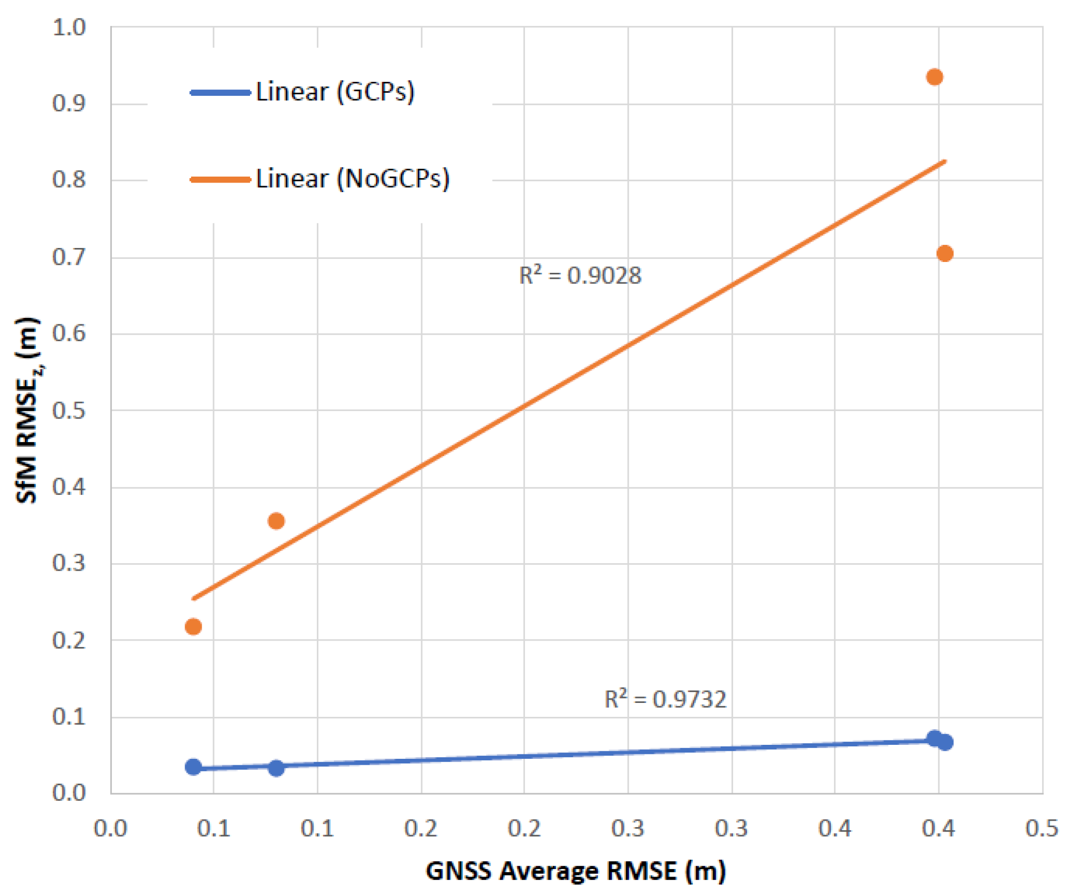
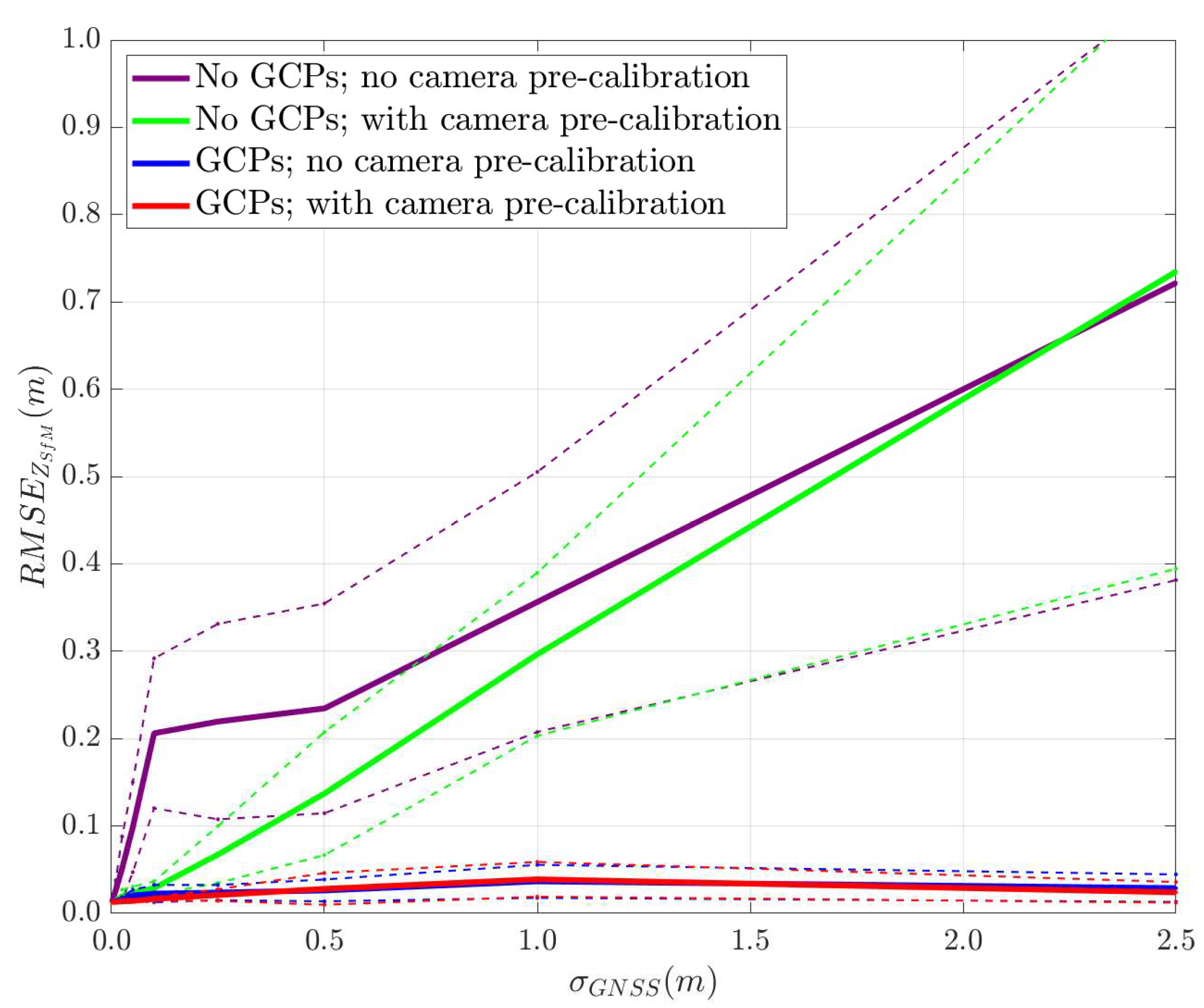
5.3. Simulation Results (simUAS)—Monte Carlo

Simulated results were obtained by using simUAS to model the relationship between GNSS and SfM point cloud accuracy. These results are shown in Figure 20, with standard uncertainty bounds (1 $\sigma$). Four cases are shown: (i) neither GCPs nor camera pre-calibration camera parameters used in SfM (purple line); (ii) no GCPs used, but camera pre-calibration parameters used in SfM (green line); (iii) GCPs used, but no camera pre-calibration used in SfM (blue line); and (iv) both GCPs and camera pre-calibration parameters used (red line). The dashed lines show the standard uncertainty bounds. In the absence of GCPs (i.e., using checkpoints only), the linear relationship is described by the equation RMSE_z = $\alpha$ × $\sigma$ + $\beta$. Here, $\alpha$ is the slope of the line, and $\beta$ is the lower bound on the SfM vertical accuracy. $\beta$ is a function of variables such as camera parameters and settings, illumination, surface texture, and processing settings. When sufficient GCPs are present, $\alpha$ is approximately equal to zero and there is no slope. When GCPs are not included, $\alpha$ is 0.29. The equation becomes RMSE_z = 0.29${\sigma }_{GNSS}$ + $\beta$.

6. Discussion

RTN GNSS was the first method tested in the Mustang Island State Park field experiment. This test used data from the Phantom 4 platform and was a very straightforward process because no post-processing of GNSS data was needed. Given that its results fulfill NOAA requirements for nautical charting, this method would be ideal in situations where RTN connection is stable.

Experiments concerning the baseline distance (for PPK GNSS) indicated that overall, RMSE_z values and baseline distances have an inverse relationship. The lowest RMSE_z values were reached when using base stations located within 30 km of the study site. Results also suggested that the variance between individual measurements increases with the baseline distance, especially when using PPK base stations located 100 km or farther away from the survey site. PPK results at 30 s resulted in a relatively higher RMSE_z for the local base (8.36 cm) compared to other stations located within 30 km (i.e., NRC at 1.87 cm, TXPO at 5.92 cm, TSAQ at 2.47 cm, and TXCC at 3.21 cm). The higher RMSE_z for the local base (8.36 cm) is likely to have been caused by displacement due to unstable ground. Although the local base was grounded, the potential for some level of motion cannot be fully discarded. For similar studies, using other tripod grounding methods (e.g., sandbags) to further restrict movement is advised. The linear, polynomial, and exponential fits of RMSE_z and baseline distance were displayed with and without the local base to account for this ground instability. The trends confirmed the interdependence between these variables. However, estimating the influence of baseline distances on the accuracy of generated products can be an unfair comparison if other contributing factors are not considered (e.g., multipath, signal obstruction, antenna quality, and weather conditions where the base stations are located).

Results from the PPK sample rate experiment showed that no single sample rate consistently provided the best results. Although higher sample rates often lead to better results, some studies have shown instances where a lower sample rate could outperform a higher one. For example, [71] tested both low-cost and geodetic-grade GNSS receivers and obtained higher vertical precision when using a 15 s sample rate compared to 1 s, 5 s, and 30 s. Other published works have examined the effects of time-depending noise errors associated with high sample rates [47,72]. Although the experiments conducted in this study ensured that GNSS receivers were placed in unobstructed locations and operated as efficiently as possible, the presence of receiver-recorded noise at the time of the surveys cannot be ruled out, and they would be more detectable at higher sample rates. In [73], researchers collected static GNSS data for four hours and used TEQC to decimate the data, originally sampled at a rate of 0.1 s, into multiple sample rates. Although their study differed slightly by using PPP GNSS corrections instead of PPK, the nature of the issue is comparable. They concluded that higher sample rates are essential for monitoring dynamic structural movements but not necessary to achieve high GNSS accuracies.

Experiments further suggest that better results may be achieved when considering both the sample rate and the PPK fix percentage. The PPK fix percentage represents the percentage of images for a given project that have been successfully corrected using fixed PPK solutions [74]. Different sample rates yield different PPK fix percentages, which in turn influence the achievable accuracy. This study showed that higher PPK fix percentages result in lower RMSE_z values, regardless of the sample rate used. This is because, in any project (and for GNSS observations at any sample rate), the accuracy of UAS-SfM-derived products improves as the number of photos that are precisely georeferenced increases.

There are several open-source services for PPP GNSS corrections, such as the Canadian Spatial Reference System-PPP and RTKLIB. However, these services can be challenging to use because there is limited information and guidance about their use for UAS mapping purposes. In addition, most do not provide synchronization capabilities between UAS image capture and human time as obtained from the PPP service. Although commercial, Inertial Explorer is an attractive alternative for PPP processing because it supports such timestamp synchronization. When using Inertial Explorer, each row of the PPP geotag solution needs to be matched manually (or programmatically, depending on the nature of the project) to its corresponding image before it can be imported into SfM software for further processing. This step differs slightly from RTN and PPK GNSS techniques, where image names and generated geotags are automatically matched. Nevertheless, PPP-corrected geotags and image names can be easily matched, as Inertial Explorer outputs them in a consistent order. In other words, the order of PPP-corrected geotags aligns with the sequence of UAS photo captures or camera events.

Results comparing the accuracy of RTN GNSS versus a total station for surveying checkpoints showed minimal differences (i.e., subcentimeter). The total station measurements were more consistent because of the reduced human error associated with them compared to RTN GNSS. While the total station measurements were more consistent between the various observations, indicated by the lower sigma values, RTN GNSS still provided lower RMSE values. Still, the total station surveyed control is only as accurate as the points it uses as reference. Because these points were established via RTN GNSS, they are inherently also influenced by the accuracy of RTN at the time they were observed. The difference of DSM maps depicted showed consistency in surface representation across most of the study area, though some discrepancies were visible along the western edge. This was caused by the difference in reach for the two systems. Because the UAS operated above the study area, it was able to map the top of the vegetation and man-made objects (i.e., picnic tables and chairs) more accurately than the TLS.

It is noteworthy that the results presented herein were influenced by the environment and terrain of the study areas. Thus, they do not guarantee consistent UAS-SfM performance across varying land covers or under different atmospheric conditions. Previous research indicates that UAS-SfM errors tend to be minimized in non-vegetated or sparsely vegetated areas, while more densely vegetated regions are subject to higher errors [75,76]. In this context, the terrain of the study sites in this research likely experienced fewer errors due to lower vegetation density. Moreover, the type of UAS also impacts the accuracy of mapping products generated via UAS-SfM accuracies. In this study, the Phantom 4 was flown at a lower altitude to achieve the same GSD as the Wingtra flight, which resulted in the Phantom capturing more photos than the Wingtra. Although these photos were captured with the same GSD, the Phantom 4 resulted in more photos than the Wingtra, which could result in capturing more subtle changes in shoreline position and elevation as well as higher point cloud density, thus increasing the density of the resulting point clouds and enhancing vertical accuracies. Compared to the Phantom 4, the Wingtra was flown at a higher altitude and speed which allowed it to complete the flight mission without swapping batteries. These likely reduced errors associated with potential changes in wind speeds or light conditions, even if such variations were minimal. Similar observations were made in previous studies [77,78]. In addition, the experiments conducted herein suggest that while design patterns using a higher sidelap percentage than overlap are often recommended [69,79], vertical accuracies within centimeters can also be accomplished when using a greater sidelap percentage than endlap, especially when surveying coastal corridors of relatively homogeneous terrain in the direction of the flight.

The experiments conducted at McNary Field and Neptune State Scenic Area suggest that the vertical accuracy of SfM point clouds, in the absence of GCPs, can be modeled as a linear function of GNSS accuracy. Additionally, both sets of results showed that, when GCPs are used, the impact of GNSS accuracy on SfM point cloud vertical accuracy is significantly reduced, as indicated by the near-flat trendline in these cases. An important observation is that, while both simulated and empirical results exhibit similar trends, the slope is significantly steeper in the empirical results than the simulated results. This steeper trend may be attributed to overly optimistic estimates of GNSS accuracy in the simulations. Additionally, the differences could result from additional error sources present in the empirical data, such as errors in camera calibration parameters, which were assumed to be perfectly known in the case of the simulated imagery. Other factors contributing to these differences include the following: first, the simulated data benefiting from a larger dataset compared to the empirical analysis and, second, the empirical results being constrained by a narrower range of GNSS accuracies, as replicating the broad range observed in the simulations is challenging in real-world experiments.

In the simulation environment, although a constant of 5 was sufficient to cause the slope α to go to zero, this result cannot be confidently generalized to real-world camera systems. This is because simUAS represents an ideal case of a near-perfect camera with several perfectly known parameters, which is not the case in the real world. In the earlier Figure 20, the inclusion of a priori camera calibration had minimal impact on accuracies when GCPs were included in the solution. However, when not using GCPs, the a priori calibration provides a clear benefit when the GNSS positioning uncertainty is low. Still, this benefit diminishes as the GNSS positioning uncertainty increases.

In summary, the results showed that the choice of georeferencing technique has a notable impact on UAS-SfM accuracies. The discrepancy between corrected and uncorrected GNSS is notable, even when using the least accurate GNSS correction techniques in this study. It must also be noted that a broader theoretical framework that models GNSS influence on the accuracy and quality of UAS-generated products could offer a more comprehensive model of GNSS influences and potentially a wider range of answers to related questions. However, GNSS performance is affected by so many factors (e.g., atmospheric conditions, quality of the receiver, satellite geometry) that modeling all these interactions is a rather complex task, especially if not oversimplifying and overgeneralizing related concepts. Therefore, the choice of parameters to investigate depends on the specific use case or application.

7. Conclusions

This study explored different GNSS georeferencing solutions for optimizing UAS-SfM data collection workflows along shorelines without the use of GCPs, and their impact on the accuracy of UAS-SfM-derived point clouds and derivative mapping products. PPK GNSS was thoroughly explored, as well as brief experiments with RTN and PPP, all direct georeferencing GNSS techniques. These methods were tested as alternatives to indirect georeferencing approaches for surveying shorelines and areas of difficult physical access. The primary focus was on using these GNSS techniques for control of UAS-SfM surveys without the use of GCPs to evaluate whether they could achieve vertical accuracies within 50 cm at the 95% confidence level, based on specifications from NOAA’s Office of Coast Survey. RTN and PPK GNSS solutions without GCPs achieved vertical accuracies that consistently met or exceeded this specification. PPP reached decimeter-level accuracies but did not fulfill requirements. More testing is needed to further improve its performance.

The baseline distance was found to be correlated with vertical errors. Stations located within 30 km of the survey site performed better than those located at greater distances. Experiments also showed that higher sample rates do not always provide the most accurate results. When determining which sample rate to use, it is advisable to first identify which sample rate provides the highest PPK fix percentage. As the results showed, higher PPK fix percentages consistently yielded lower RMSEs irrespective of the sample rate. In terms of secondary experiments, higher precision in vertical accuracy was obtained when using checkpoints surveyed with a total station instead of RTN GNSS. The absolute accuracy of the total station survey depended on the RTN GNSS, because of the establishment of temporary control points that require RTN GNSS. A popular discussion today is whether UAS-SfM can substitute traditional techniques for topographic mapping. This study showed very close results when obtaining heights using RTN GNSS and UAS-SfM, which suggests that substitution is indeed possible in some cases. Finally, the DSMs from UAS-SfM were very similar over exposed ground to those from a TLS, except in vegetated features and man-made objects due to scanner occlusion and differences in the oblique perspective of TLS versus the nadir perspective of UAS-SfM, such as along the edges of structures. In more complex, rugged and/or vegetated terrain with more occlusions from the ground or other structures, and over larger areas, TLS will require more observation stations. As such, UAS-SfM is typically more efficient for point cloud data collection relative to TLS in these situations.

Monte Carlo simulations and empirical testing showed that the vertical accuracy of point clouds generated using UAS is well modeled as a linear function of the GNSS accuracy when no GCPs are used. A less significant effect is observed when GCPs are present. Although both the simulated and empirical results have similar trends, the slope of best-fit lines is steeper with the latter, potentially because real-world data collection inevitably incurs additional error sources that can be eliminated in simulation (e.g., due to lighting and calibration parameters). In addition, the empirical results are impacted by a wider range of GNSS accuracies, as it is challenging to reproduce the perfect conditions that can be modeled in simulation.

Finally, the use of GNSS solutions for georeferencing herein explored greatly reduced the amount of time taken for UAS-SfM data acquisition. Eliminating reliance on GCPs means that no time is invested into distributing GCPs across the survey area and taking measurements on them; thus, no time is needed to mark them during post-processing, further expediting the process of UAS surveying. The results discussed in this study are limited to the survey sites and equipment used, and the overall conditions at the survey sites. Further research is recommended to test the methods in vastly differing coastal morphologies. Additionally, future work is recommended to more extensively explore the applicability of PPP for UAS surveys. This work could test various data collection procedures, such as allowing the UAS platform to stand static for some time before deployment. In summary, the results and findings presented in this study are applicable to those seeking to adopt efficient UAS-SfM data collection workflows relying on GNSS georeferencing solutions for coastal zone monitoring and other survey applications.

References

1. James, M.R.; Robson, S. Straightforward reconstruction of 3D surfaces and topography with a camera: Accuracy and geoscience application. J. Geophys. Res. Earth Surf. 2012, 117, F3. [Google Scholar] [CrossRef]
2. Javadnejad, F.; Slocum, R.K.; Gillins, D.T.; Olsen, M.J.; Parrish, C.E. Dense point cloud quality factor as proxy for accuracy assessment of image-based 3D reconstruction. J. Surv. Eng. 2021, 147, 04020021. [Google Scholar] [CrossRef]
3. Casella, E.; Lewin, P.; Ghilardi, M.; Rovere, A.; Bejarano, S. Assessing the relative accuracy of coral heights reconstructed from drones and structure from motion photogrammetry on coral reefs. Coral Reefs 2022, 41, 869–875. [Google Scholar] [CrossRef]
4. Śledziowski, J.; Terefenko, P.; Giza, A.; Forczmański, P.; Łysko, A.; Maćków, W.; Stępień, G.; Tomczak, A.; Kurylczyk, A. Application of unmanned aerial vehicles and image processing techniques in monitoring underwater coastal protection measures. Remote Sens. 2022, 14, 458. [Google Scholar] [CrossRef]
5. Pashaei, M.; Kamangir, H.; Starek, M.J.; Tissot, P. Review and evaluation of deep learning architectures for efficient land cover mapping with UAS hyper-spatial imagery: A case study over a wetland. Remote Sens. 2020, 12, 959. [Google Scholar] [CrossRef]
6. Mancini, F.; Dubbini, M.; Gattelli, M.; Stecchi, F.; Fabbri, S.; Gabbianelli, G. Using unmanned aerial vehicles (UAV) for high-resolution reconstruction of topography: The structure from motion approach on coastal environments. Remote Sens. 2013, 5, 6880–6898. [Google Scholar] [CrossRef]
7. Albeaino, G.; Kelly, C.R.; Lassiter, H.A.; Wilkinson, B.; Gheisari, M.; Issa, R.R. Quantitative and qualitative assessments of geometric feature accuracy using a UAS-Lidar system for building surveying applications. J. Archit. Eng. 2023, 29, 04022046. [Google Scholar] [CrossRef]
8. Ballouch, Z.; Hajji, R.; Poux, F.; Kharroubi, A.; Billen, R. A prior level fusion approach for the semantic segmentation of 3D point clouds using deep learning. Remote Sens. 2022, 14, 3415. [Google Scholar] [CrossRef]
9. Williams, A.T.; Rangel-Buitrago, N.; Pranzini, E.; Anfuso, G. The management of coastal erosion. Ocean. Coast. Manag. 2018, 156, 4–20. [Google Scholar] [CrossRef]
10. López, L.; Cellone, F. SfM-MVS and GIS analysis of shoreline changes in a coastal wetland, Parque Costero del Sur Biosphere Reserve, Argentina. Geocarto Int. 2022, 37, 11134–11150. [Google Scholar] [CrossRef]
11. Casella, E.; Rovere, A.; Pedroncini, A.; Stark, C.P.; Casella, M.; Ferrari, M.; Firpo, M. Drones as tools for monitoring beach topography changes in the Ligurian Sea (NW Mediterranean). Geo-Mar. Lett. 2016, 36, 151–163. [Google Scholar] [CrossRef]
12. Hwang, B.H.; Do, K.D.; Chang, S.Y. Morphological response of Storm Hinnamnor at Songjeong Beach using UAV-derived data. J. Coast. Res. 2024, 116, 126–130. [Google Scholar] [CrossRef]
13. Sturdivant, E.J.; Lentz, E.E.; Thieler, E.R.; Farris, A.S.; Weber, K.M.; Remsen, D.P.; Miner, S.; Henderson, R.E. UAS-SfM for coastal research: Geomorphic feature extraction and land cover classification from high-resolution elevation and optical imagery. Remote Sens. 2017, 9, 1020. [Google Scholar] [CrossRef]
14. Gonçalves, J.A.; Henriques, R. UAV photogrammetry for topographic monitoring of coastal areas. ISPRS J. Photogramm. Remote Sens. 2015, 104, 101–111. [Google Scholar] [CrossRef]
15. Shin, B.S.; Kim, K.H. Dynamic observation for terrain volume estimation using UAV-based photogrammetry. J. Coast. Res. 2024, 116, 658–662. [Google Scholar] [CrossRef]
16. Klemas, V.V. Coastal and environmental remote sensing from unmanned aerial vehicles: An overview. J. Coast. Res. 2015, 31, 1260–1267. [Google Scholar] [CrossRef]
17. Westoby, M.J.; Brasington, J.; Glasser, N.F.; Hambrey, M.J.; Reynolds, J.M. ‘Structure-from-Motion’ photogrammetry: A low-cost, effective tool for geoscience applications. Geomorphology 2012, 179, 300–314. [Google Scholar] [CrossRef]
18. Jakovljevic, G.; Govedarica, M.; Alvarez-Taboada, F.; Pajic, V. Accuracy assessment of deep learning based classification of LiDAR and UAV points clouds for DTM creation and flood risk mapping. Geosciences 2019, 9, 323. [Google Scholar] [CrossRef]
19. Carrera-Hernández, J.; Levresse, G.; Lacan, P. Is UAV-SfM surveying ready to replace traditional surveying techniques? Int. J. Remote Sens. 2020, 41, 4820–4837. [Google Scholar] [CrossRef]
20. Rogers, S.R.; Manning, I.; Livingstone, W. Comparing the spatial accuracy of digital surface models from four unoccupied aerial systems: Photogrammetry versus LiDAR. Remote Sens. 2020, 12, 2806. [Google Scholar] [CrossRef]
21. Fraser, C.S. Automatic camera calibration in close range photogrammetry. Photogramm. Eng. Remote Sens. 2013, 79, 381–388. [Google Scholar] [CrossRef]
22. Ajayi, O.G.; Salubi, A.A.; Angbas, A.F.; Odigure, M.G. Generation of accurate digital elevation models from UAV acquired low percentage overlapping images. Int. J. Remote Sens. 2017, 38, 3113–3134. [Google Scholar] [CrossRef]
23. Chang, A.; Jung, J.; Maeda, M.M.; Landivar, J. Crop height monitoring with digital imagery from unmanned aerial system (UAS). Comput. Electron. Agric. 2017, 141, 232–237. [Google Scholar] [CrossRef]
24. Sanz-Ablanedo, E.; Chandler, J.H.; Rodríguez-Pérez, J.R.; Ordóñez, C. Accuracy of unmanned aerial vehicle (UAV) and SfM photogrammetry survey as a function of the number and location of ground control points used. Remote Sens. 2018, 10, 1606. [Google Scholar] [CrossRef]
25. Thomas, O.; Stallings, C.; Wilkinson, B. Unmanned aerial vehicles can accurately, reliably, and economically compete with terrestrial mapping methods. J. Unmanned Veh. Syst. 2019, 8, 57–74. [Google Scholar] [CrossRef]
26. Mugnai, F.; Tucci, G. A comparative analysis of unmanned aircraft systems in low altitude photogrammetric surveys. Remote Sens. 2022, 14, 726. [Google Scholar] [CrossRef]
27. Ye, S.; Yan, F.; Zhang, Q.; Shen, D. Comparing the accuracies of sUAV-SFM and UAV-LiDAR point clouds for topographic measurements. Arab. J. Geosci. 2022, 15, 388. [Google Scholar] [CrossRef]
28. Rabah, M.; Basiouny, M.; Ghanem, E.; Elhadary, A. Using RTK and VRS in direct geo-referencing of the UAV imagery. NRIAG J. Astron. Geophys. 2018, 7, 220–226. [Google Scholar] [CrossRef]
29. Oniga, V.E.; Breaban, A.I.; Statescu, F. Determining the optimum number of ground control points for obtaining high precision results based on UAS images. Proceedings 2018, 2, 352. [Google Scholar] [CrossRef]
30. Padró, J.C.; Muñoz, F.J.; Planas, J.; Pons, X. Comparison of four UAV georeferencing methods for environmental monitoring purposes focusing on the combined use with airborne and satellite remote sensing platforms. Int. J. Appl. Earth Obs. Geoinf. 2019, 75, 130–140. [Google Scholar] [CrossRef]
31. Nesbit, P.R.; Hubbard, S.M.; Hugenholtz, C.H. Direct georeferencing UAV-SfM in high-relief topography: Accuracy assessment and alternative ground control strategies along steep inaccessible rock slopes. Remote Sens. 2022, 14, 490. [Google Scholar] [CrossRef]
32. Zhang, H.; Aldana-Jague, E.; Clapuyt, F.; Wilken, F.; Vanacker, V.; Van Oost, K. Evaluating the potential of post-processing kinematic (PPK) georeferencing for UAV-based structure-from-motion (SfM) photogrammetry and surface change detection. EArth Surf. Dyn. 2019, 7, 807–827. [Google Scholar] [CrossRef]
33. Gurturk, M.; Soycan, M. Accuracy assessment of kinematic PPP versus PPK for GNSS flights data processing. Surv. Rev. 2022, 54, 48–56. [Google Scholar] [CrossRef]
34. Allahyari, M.; Olsen, M.J.; Gillins, D.T.; Dennis, M.L. Tale of two RTNs: Rigorous evaluation of real-time network GNSS observations. J. Surv. Eng. 2018, 144, 05018001. [Google Scholar] [CrossRef]
35. Raza, S.; Al-Kaisy, A.; Teixeira, R.; Meyer, B. The role of GNSS-RTN in transportation applications. Encyclopedia 2020, 2, 83. [Google Scholar] [CrossRef]
36. Rokaha, B.; Gautam, B.P.; Kitani, T. Building a reliable and cost-effective RTK-GNSS infrastructure for precise positioning of IoT applications. In Proceedings of the Twelfth International Conference on Mobile Computing and Ubiquitous Network (ICMU), Kathmandu, Nepal, 4–6 November 2019; pp. 1–4. [Google Scholar] [CrossRef]
37. Huang, G.; Du, S.; Wang, D. GNSS techniques for real-time monitoring of landslides: A review. Satellite Navigation 2023, 4, 5. [Google Scholar] [CrossRef]
38. Miller, Z.M.; Hupy, J.; Chandrasekaran, A.; Shao, G.; Fei, S. Application of postprocessing kinematic methods with UAS remote sensing in forest ecosystems. J. For. 2021, 119, 454–466. [Google Scholar] [CrossRef]
39. Van Sickle, J. GPS for Land Surveyors; CRC Press: Boca Raton, FL, USA, 2015. [Google Scholar] [CrossRef]
40. Anquela, A.; Martín, A.; Berné, J.; Padín, J. GPS and GLONASS static and kinematic PPP results. J. Surv. Eng. 2013, 139, 47–58. [Google Scholar] [CrossRef]
41. Angrisano, A.; Dardanelli, G.; Innac, A.; Pisciotta, A.; Pipitone, C.; Gaglione, S. Performance assessment of PPP surveys with open source software using the GNSS GPS–GLONASS–Galileo constellations. Appl. Sci. 2020, 10, 5420. [Google Scholar] [CrossRef]
42. Henkel, P.; Iafrancesco, M.; Sperl, A. Precise point positioning with multipath estimation. In Proceedings of the 2016 IEEE/ION Position, Location and Navigation Symposium (PLANS), Savannah, GA, USA, 11–14 April 2016; pp. 144–149. [Google Scholar] [CrossRef]
43. Alkan, R.M.; Saka, M.H.; Ozulu, İ.M.; İlçi, V. Kinematic precise point positioning using GPS and GLONASS measurements in marine environments. Measurement 2017, 109, 36–43. [Google Scholar] [CrossRef]
44. Chen, C.; Chang, G. PPPLib: An open-source software for precise point positioning using GPS, BeiDou, Galileo, GLONASS, and QZSS with multi-frequency observations. GPS Solut. 2021, 25, 18. [Google Scholar] [CrossRef]
45. Turner, D.; Lucieer, A.; Wallace, L. Direct georeferencing of ultrahigh-resolution UAV imagery. IEEE Trans. Geosci. Remote Sens. 2013, 52, 2738–2745. [Google Scholar] [CrossRef]
46. Daakir, M.; Pierrot-Deseilligny, M.; Bosser, P.; Pichard, F.; Thom, C.; Rabot, Y.; Martin, O. Lightweight UAV with on-board photogrammetry and single-frequency GPS positioning for metrology applications. ISPRS J. Photogramm. Remote Sens. 2017, 127, 115–126. [Google Scholar] [CrossRef]
47. Groves, P.D. Principles of GNSS, inertial, and multisensor integrated navigation systems, [Book review]. IEEE Aerosp. Electron. Syst. Mag. 2015, 30, 26–27. [Google Scholar] [CrossRef]
48. Lu, F.; Li, J. Precise point positioning study to use different IGS precise ephemeris. In Proceedings of the 2011 IEEE International Conference on Computer Science and Automation Engineering, Shanghai, China, 10–12 June 2011; Volume 3. [Google Scholar] [CrossRef]
49. Zhang, Y.; Yu, W.; Han, Y.; Hong, Z.; Shen, S.; Yang, S.; Wang, J. Static and kinematic positioning performance of a low-cost real-time kinematic navigation system module. Adv. Space Res. 2019, 63, 3029–3042. [Google Scholar] [CrossRef]
50. Forlani, G.; Dall’Asta, E.; Diotri, F.; Morra di Cella, U.; Roncella, R.; Santise, M. Quality assessment of DSMs produced from UAV flights georeferenced with on-board RTK positioning. Remote Sens. 2018, 10, 311. [Google Scholar] [CrossRef]
51. Stott, E.; Williams, R.D.; Hoey, T.B. Ground control point distribution for accurate kilometre-scale topographic mapping using an RTK-GNSS unmanned aerial vehicle and SfM photogrammetry. Drones 2020, 4, 55. [Google Scholar] [CrossRef]
52. Kalacska, M.; Lucanus, O.; Arroyo-Mora, J.P.; Laliberté, É.; Elmer, K.; Leblanc, G.; Groves, A. Accuracy of 3D landscape reconstruction without ground control points using different UAS platforms. Drones 2020, 4, 13. [Google Scholar] [CrossRef]
53. Raychaudhuri, S. Introduction to Monte Carlo simulation. In Proceedings of the 2008 Winter Simulation Conference, Miami, FL, USA, 7–10 December 2008. [Google Scholar] [CrossRef]
54. Carbonneau, P.E.; Dietrich, J.T. Cost-effective non-metric photogrammetry from consumer-grade sUAS: Implications for direct georeferencing of structure from motion photogrammetry. Earth Surf. Process. Landforms 2016, 42, 473–486. [Google Scholar] [CrossRef]
55. Slocum, R.K.; Parrish, C.E. Simulated imagery rendering workflow for UAS-based photogrammetric 3D reconstruction accuracy assessments. Remote Sens. 2017, 9, 396. [Google Scholar] [CrossRef]
56. Li, T.; Zhang, B.; Cheng, X.; Westoby, M.J.; Li, Z.; Ma, C.; Hui, F.; Shokr, M.; Liu, Y.; Chen, Z.; et al. Resolving fine-scale surface features on polar sea ice: A first assessment of UAS photogrammetry without ground control. Remote Sens. 2019, 11, 784. [Google Scholar] [CrossRef]
57. National Oceanic and Atmospheric Administration. Hydrographic Surveys Specifications and Deliverables. 2022. Available online: https://www.nauticalcharts.noaa.gov/publications/docs/standards-and-requirements/specs/HSSD_2022.pdf (accessed on 1 August 2024).
58. Pilartes-Congo, J.; Starek, M.J.; Berryhill, J. Impact of different GNSS solutions on UAS-SfM vertical accuracy for shoreline charting. In Proceedings of the IGARSS 2023—2023 IEEE International Geoscience and Remote Sensing Symposium, Pasadena, CA, USA, 16–21 July 2023; pp. 4666–4669. [Google Scholar] [CrossRef]
59. Wingtra. WingtraOne Drone: Technical Specifications. Available online: https://wingtra.com/mapping-drone-wingtraone/technical-specifications/ (accessed on 13 June 2021).
60. DJI. Phantom 4 RTK User Manual v2.4. Available online: https://dl.djicdn.com/downloads/phantom_4_rtk/20200721/Phantom_4_RTK_User_Manual_v2.4_EN.pdf (accessed on 10 October 2024).
61. Septentrio. Altus NR3 User Manual. Available online: https://globalgpssystems.com/wp-content/uploads/2020/03/altus_nr3.pdf (accessed on 10 October 2024).
62. Fuegner, A. TxDOT GPS Applications. Available online: https://www.gps.gov/cgsic/states/2012/austin/fuegner.pdf (accessed on 6 October 2024).
63. Smith, D.; Choi, K.; Prouty, D.; Jordan, K.; Henning, W. Analysis of the TXDOT RTN and OPUS-RS from the geoid slope validation survey of 2011: Case study for Texas. J. Surv. Eng. 2014, 140, 05014003. [Google Scholar] [CrossRef]
64. Juniper Systems, I. Allegro 2 Owner’s Manual. Available online: https://junipersys.com/data/support/allegro-2-manual-english.pdf (accessed on 10 October 2024).
65. RIEGL. RIEGL VZ-2000i. Available online: http://www.riegl.com/nc/products/terrestrial-scanning/produktdetail/product/scanner/58/ (accessed on 13 May 2024).
66. Leica. Leica TS11/TS15 User Manual. Available online: http://www.engineeringsurveyor.com/software/Leica_Viva_TS11_TS15_User_Manual.pdf (accessed on 18 December 2022).
67. Leica. Leica Geosystems Original Accessories: Material Matters. Available online: https://leica-geosystems.com/services-and-support/-/media/files/archived-files/2793c068-e703-4900-a20d-e5e6bba8978e.pdf (accessed on 11 October 2024).
68. ASPRS. ASPRS positional accuracy standards for digital geospatial data. Photogramm. Eng. Remote Sens. 2015, 81, A1–A26. [Google Scholar] [CrossRef]
69. Over, J.S.R.; Ritchie, A.C.; Kranenburg, C.J.; Brown, J.A.; Buscombe, D.D.; Noble, T.; Sherwood, C.R.; Warrick, J.A.; Wernette, P.A. Processing Coastal Imagery with Agisoft Metashape Professional Edition, Version 1.6—Structure from Motion Workflow Documentation; Technical Report; US Geological Survey: Reston, VA, USA, 2021. [CrossRef]
70. Agisoft. Agisoft Metashape User Manual: Professional Edition, Version 1.8. Available online: https://www.agisoft.com/pdf/metashape-pro_1_8_en.pdf (accessed on 17 October 2024).
71. Romero-Andrade, R.; Trejo-Soto, M.E.; Vázquez-Ontiveros, J.R.; Hernández-Andrade, D.; Cabanillas-Zavala, J.L. Sampling rate impact on precise point positioning with a low-cost GNSS receiver. Appl. Sci. 2021, 11, 7669. [Google Scholar] [CrossRef]
72. Zhang, Q.; Niu, X.; Shi, C. Assessment of the effect of GNSS sampling rate on GNSS/INS relative accuracy on different time scales for precision measurements. Measurement 2019, 145, 583–593. [Google Scholar] [CrossRef]
73. Erol, S.; Alkan, R.M.; Ozulu, İ.M.; Ilçi, V. Impact of different sampling rates on precise point positioning performance using online processing service. Geo-Spat. Inf. Sci. 2021, 24, 302–312. [Google Scholar] [CrossRef]
74. Wingtra. PPK Geotagging. Available online: https://knowledge.wingtra.com/en/ppk-geotagging (accessed on 1 April 2022).
75. Carrivick, J.L.; Smith, M.W.; Quincey, D.J. Structure from Motion in the Geosciences; John Wiley & Sons: Hoboken, NJ, USA, 2016. [Google Scholar]
76. Salach, A.; Bakuła, K.; Pilarska, M.; Ostrowski, W.; Górski, K.; Kurczyński, Z. Accuracy assessment of point clouds from LiDAR and dense image matching acquired using the UAV platform for DTM creation. ISPRS Int. J.-Geo-Inf. 2018, 7, 342. [Google Scholar] [CrossRef]
77. Deliry, S.I.; Avdan, U. Accuracy of unmanned aerial systems photogrammetry and structure from motion in surveying and mapping: A review. J. Indian Soc. Remote Sens. 2021, 49, 1997–2017. [Google Scholar] [CrossRef]
78. Liu, Y.; Han, K.; Rasdorf, W. Assessment and prediction of impact of flight configuration factors on UAS-based photogrammetric survey accuracy. Remote Sens. 2022, 14, 4119. [Google Scholar] [CrossRef]
79. Jiménez-Jiménez, S.I.; Ojeda-Bustamante, W.; Marcial-Pablo, M.d.J.; Enciso, J. Digital terrain models generated with low-cost UAV photogrammetry: Methodology and accuracy. ISPRS Int. J.-Geo-Inf. 2021, 10, 285. [Google Scholar] [CrossRef]
Figure 1. Mustang Island State Park, Texas. Source of basemap: ESRI.
Drones 08 00646 g001
Figure 2. (a) McNary Field; (b) Neptune State Scenic Area. Source of basemap: ESRI.
Drones 08 00646 g002
Figure 3. (a) WingtraOne PPK UAS; (b) DJI Phantom 4 RTK UAS.
Drones 08 00646 g003
Figure 4. (a) Aerial target; (b) NR3 GNSS receiver; (c) Allegro 2 data collector; (d) Reigl VZ-2000i TLS; (e) TS15 P 1″ robotic total station; (f) Leica GPR111 circular prism.
Drones 08 00646 g004
Figure 5. Checkpoint distribution at Mustang Island State Park.
Drones 08 00646 g005
Figure 6. Map of cross-shore beach topography transects (i.e., height profiles).
Drones 08 00646 g006
Figure 7. Flowchart summarizing the GNSS evaluation workflow.
Drones 08 00646 g007
Figure 8. Base stations used for PPK corrections of the Mustang Island State Park UAS imagery and their respective distances relative to the survey site. Source of basemap: ESRI.
Drones 08 00646 g008
Figure 9. (a) DJI Phantom 4 RTK in action; (b) example of center eyelet aerial target; (c) survey crew member carrying a circular prism attached to a survey rod; (d) Leica TS15P 1″ total station.
Drones 08 00646 g009
Figure 10. Control and checkpoint distribution at McNary Field. Source of basemap: ESRI.
Drones 08 00646 g010
Figure 11. GCP and checkpoint distribution at Neptune State Scenic Area.
Drones 08 00646 g011
Figure 12. Simplified version of the simUAS workflow. Subfigure (A) shows the simulated scene, camera stations (yellow dots), and illumination; (B) shows the rendered imagery of the scene using the Blender Internal Render Engine; (C) shows the point cloud generated by processing the imagery through SfM software; (D) depicts the process of conducting the accuracy assessment by comparing the point cloud against the original simulated scene.
Drones 08 00646 g012
Figure 13. Variation in (a) RMSEz and (b) Standard Deviationz values according to the sample rate for all base stations considered in this study.
Drones 08 00646 g013
Figure 14. Variation in (a) RMSEz and (b) Standard Deviationz values according to the sample rate for base stations located within 30 km.
Drones 08 00646 g014
Figure 15. Linear, polynomial, and exponential fits between RMSEz values at 1 s and 30 s sample rates.
Drones 08 00646 g015
Figure 16. PPK fix percentage versus RMSEz values at different sample rates.
Drones 08 00646 g016
Figure 17. DSMs and DSM of difference at Mustang Island State Park: (a) UAS-SfM DSM; (b) TLS DSM; and (c) DSM of difference.
Drones 08 00646 g017
Figure 18. Height differences between RTN GNSS and UAS DSM.
Drones 08 00646 g018
Figure 19. Results of empirical accuracy assessment.
Drones 08 00646 g019
Figure 20. Modeled relationship between the SfM point cloud accuracy and GNSS positioning accuracy from simUAS Monte Carlo analysis.
Drones 08 00646 g020