Hybrid Dual-Scale Neural Network Model for Tracking Complex Maneuvering UAVs

Abstract

Accurate tracking and predicting unmanned aerial vehicle (UAV) trajectories are essential to ensure mission success, equipment safety, and data accuracy. Maneuverable UAVs exhibit complex and dynamic motion, and conventional tracking algorithms that rely on predefined models perform poorly when unknown parameters are used. To address this issue, this paper introduces a hybrid dual-scale neural network model based on the generalized regression multi-model and cubature information filter (GRMM-CIF) framework. We have established the GRMM-CIF filtering structure to differentiate motion modes and reduce measurement noise. Furthermore, considering trajectory datasets and rates of motion change, a neural network at different scales will be designed. We propose the dual-scale bidirectional long short-term memory (DS-Bi-LSTM) algorithm to address prediction delays in a multi-model context. Additionally, we employ scale sliding windows and threshold-based decision-making to achieve dual-scale trajectory reconstruction, ultimately enhancing tracking accuracy. Simulation results confirm the effectiveness of our approach in handling the uncertainty of UAV motion and achieving precise estimations.

1. Introduction

Unmanned aerial vehicles (UAVs) are integral in various fields, including aerial photography, logistics, search, and rescue missions [1]. Tracking moving targets is essential to ensure effective UAV mission execution, maintain steady tracking of the target, and provide the necessary data and information for decision-making [2]. However, the maneuvering performance and behavior of UAVs may be affected by a variety of factors, such as wind, manipulator’s intent, and environmental influences, resulting in varied and unpredictable motion patterns. Therefore, the tracking algorithms are difficult to establish accurate models in advance [3,4].

Since the last decade, scientists have been exploring various approaches to tracking targets [5,6]. UAV states are described using dynamic equations, with parameters incorporated into the state vector dimensions to facilitate joint estimation [7]. Past work has made significant advances in effectively solving the problem of target tracking, however, the robustness and convergence of these algorithms directly depend on accurate initial state estimation of process and measurement noise, unknown parameters, and covariance matrices [8,9,10]. As technology advances, modern target tracking environments become increasingly complex, which further increases the difficulty of tracking tasks [11]. To overcome this challenge, several improved extension and modification models from traditional interactive multimodal model (IMM) algorithms were proposed [12]. For instance, Wonkeun et al. suggested an adaptive Kalman filter IMM (AKF-IMM) to estimate the unknown time-varying measurement loss probability adaptively [13]. Adaptive target tracking of IMM with heterogeneous velocity representation and linear/curved motion model was proposed in [14]. Lu et al. derived an adaptive IMM filter for jump Markov systems with inaccurate noise covariances and missing measurements based on Kullback–Leibler average (KLA) [15]. While these extensions improve state estimation accuracy by dynamically adjusting the model and covariance matrix, they are limited by particular maneuvering target models [16,17,18].

Data-driven approaches do not require prior knowledge or models, they can automatically extract features from data and make predictions by learning patterns and relationships between input data [19,20,21]. For instance, algorithms such as long short-term memory (LSTM) [22] in deep learning have shown promising results in target tracking applications. These algorithms possess the ability to capture and learn long-term dependencies, enabling them to capture better the dynamic characteristics of target motion [23].

However, in contrast to model-driven methods, data-driven approaches necessitate extensive datasets for efficient model training, and the efficacy of models is significantly contingent on data quality and quantity [24,25]. In addition, data-driven methods also have problems such as overfitting or instability. For the traditional MM algorithm [26], an appropriate model based on an estimate of previous observations always needs to catch up to the current target state [27], causing performance deterioration, especially for highly maneuverable targets or unpredictable target movements. Therefore, future research can explore combining model-driven and data-driven approaches to achieve better target tracking [28]. This may involve combining data-driven techniques with traditional physical models to understand the target’s motion and maneuvering better, improving tracking accuracy and robustness [29].

In this paper, we propose a multi-model tracking method based on dual-scale deep learning within the framework of generalized regression multi-model (GRMM) and cubature information filter (CIF) [30], which is applicable to multiple targets with complex maneuvering motions. Unlike the aforementioned approaches, this method combines model-driven and data-driven schemes to improve tracking accuracy and robustness. The primary contributions of this approach are as follows:

• To improve the multi-model algorithm of the Markov transfer chain, GRMM provides an effective Markov transfer matrix according to the database when the prior parameters of maneuvering UAVs are unknown, which improves the discrimination of the motion state of the maneuvering target and uses CIF nonlinear filtering to filter the measured value to improve the tracking accuracy of the maneuvering UAVs.
• We design a dual-scale Bi-LSTM network to correct state delay and improve the state estimation of the filter for maneuvering UAVs. This structure considers the temporal relationships of the maneuvering target’s state vector at different scales, which enhances the filter’s adaptability to complex maneuvering motions and reduces tracking errors caused by delays.

This manuscript is organized as follows: Section 2 provides a brief analysis of the motion characteristics of the maneuvering target and presents the mathematical modeling of the maneuvering target. Section 3 introduces the dual-scale neural network prediction algorithm under the multi-model filtering framework to deal with the delay problem of the maneuvering target state transition. Section 4 validates the effectiveness of the proposed methodology. Multi-model adaptive tracking prediction method through simulation experiments and our conclusions are presented in Section 5.

2. Target Tracking Problem Definition

2.1. Nonlinear Motion Mode of Maneuvering Targets

This paper considers a three-dimensional (3D) plane coordinate of UAV tracking. Thus, ${\mathit{x}}_k$ is defined as ${[{\xi }_k, {\dot{\xi }}_k, {\ddot{\xi }}_k, {\upsilon }_k, {\dot{\upsilon }}_k, {\ddot{\upsilon }}_k, {\zeta }_k, {\dot{\zeta }}_k, {\ddot{\zeta }}_k]}^{\mathrm{T}}$, where ${[{\xi }_k, {\upsilon }_k, {\zeta }_k]}^{\mathrm{T}}$ is the target 3D position in Cartesian coordinates, ${[{\dot{\xi }}_k, {\dot{\upsilon }}_k, {\dot{\zeta }}_k]}^{\mathrm{T}}$ is the corresponding velocity of target, and ${[{\ddot{\xi }}_k, {\ddot{\upsilon }}_k, {\ddot{\zeta }}_k]}^{\mathrm{T}}$ is the target’s accelerated speed.

In real-world scenarios, state estimation for UAV tracking can be considered as a discrete-time nonlinear dynamic system [26].

$${\mathit{x}}_{k+1}=\mathit{f}({\mathit{x}}_k,{\mathit{u}}_k)+{\mathit{\eta }}_k$$

(1)

where ${\mathit{x}}_{k+1}\in {ℝ}^n$ denote the state vector of the system at time $k$, $\mathit{f}$ is vector-valued (possibly time-varying) functions, and $n$ is a positive integer. ${\mathit{u}}_k$ represents the control input at time step $k$, as for the weak maneuvering trajectory, we can ignore it in the state transition equation [29]. ${\mathit{\eta }}_k$ is the zero-mean Gaussian noise. The process noise ${\mathit{\eta }}_k$ can impact various components of the state vector ${\mathit{x}}_k$ such as velocity, distance, and other relevant parameters.

The discrete-time equivalent of the above continuous-time model is

$${\mathit{x}}_{k+1}=diag[F,F,F]{\mathit{x}}_k+{\mathit{\eta }}_k$$

(2)

The transition matrix $\mathit{F}$ is defined as three shapes, ${\mathit{F}}_{}^{\mathrm{CV}}$ constant velocity (CV) state, ${\mathit{F}}_{}^{\mathrm{CA}}$ constant accelerated (CA) state, and ${\mathit{F}}_{}^{\mathrm{CT}}$ constant-turn (CT) state, to satisfy the requirement in generating maneuvering target trajectories. According to [26], the CV mode is defined as

$${\mathit{F}}_k^{cv}=\left[\begin{array}{ccc}1& \Delta \tau & 0\\ 0& 1& 0\\ 0& 0& 0\end{array}\right] {\mathit{F}}_{}^{\mathrm{CV}}(k)\triangleq diag\left[F_k^{cv},F_k^{cv},F_k^{cv}\right]$$

(3)

where $\Delta \tau$ represents the time step. In matrix theory, $diag$ commonly refers to a diagonal matrix. ${\mathit{F}}_k^{cv}$, ${\mathit{F}}_k^{ca}$, ${\mathit{F}}_k^{ct}$ represent 3 × 3 subtransition matrices corresponding to specific motion models (CV, CA, or CT) which maneuvering target can follow during 3D tracking, the resulting block diagonal matrix ${\mathit{F}}_{}^{\mathrm{CV}}(k)$, ${\mathit{F}}_{}^{\mathrm{CA}}(k)$, ${\mathit{F}}_{}^{\mathrm{CT}}(k)$ will be 9 × 9 matrices.

In the context of UAVs in cruising mode, we define the CA mode as.

$${\mathit{F}}_k^{ca}=\left[\begin{array}{ccc}1& \Delta \tau & \Delta {\tau }^2/2\\ 0& 1& \mathrm{T}\\ 0& 1& \mathrm{T}\end{array}\right] {\mathit{F}}_{}^{\mathrm{CA}}(k)\triangleq diag\left[F_k^{ca},F_k^{ca},F_k^{ca}\right]$$

(4)

In the context of UAVs in cruising mode, we define the CT mode as.

$${\mathit{F}}_k^{ct}=\left[\begin{array}{ccc}1& \frac{\sin ({\omega }_m\Delta \tau )}{{\omega }_m}& \frac{1-\cos ({\omega }_m\Delta \tau )}{{\omega }_{{}_m}^2}\\ 0& \cos ({\omega }_m\Delta \tau )& \frac{\sin ({\omega }_m\Delta \tau )}{{\omega }_m}\\ 0& -{\omega }_m\sin ({\omega }_m\Delta \tau )& \cos ({\omega }_m\Delta \tau )\end{array}\right] {\mathit{F}}_{}^{\mathrm{CT}}(k)\triangleq diag\left[F_k^{ct},F_k^{ct},F_k^{ct}\right]$$

(5)

where ${\omega }_m$ denotes the turn rate for the constant-turn mode.

The measurement vector of system at time $k$, ${\mathit{y}}_k\in {ℝ}^m$, can be expressed as

$${\mathit{y}}_k={\mathit{H}}_k({\mathit{x}}_k)+{\mathit{n}}_k$$

(6)

$$\underset{{\mathit{y}}_k}{\underbrace{\left[\begin{array}{c}{r}_k\\ v_k\\ {\phi }_k\\ {\theta }_k\end{array}\right]}}=\underset{{\mathit{H}}_k({\mathit{x}}_k)}{\underbrace{\left[\begin{array}{c}\sqrt{{({\xi }_k-{\xi }_k^{\mathrm{R}})}^2+{({\upsilon }_k-{\upsilon }_k^{\mathrm{R}})}^2+{({\zeta }_k-{\zeta }_k^{\mathrm{R}})}^2}\\ \frac{({\xi }_k-{\xi }_k^{\mathrm{R}}){\dot{\xi }}_k+({\upsilon }_k-{\upsilon }_k^{\mathrm{R}}){\dot{\upsilon }}_k+({\zeta }_k-{\zeta }_k^{\mathrm{R}}){\dot{\zeta }}_k}{\sqrt{{({\xi }_k-{\xi }_k^{\mathrm{R}})}^2+{({\upsilon }_k-{\upsilon }_k^{\mathrm{R}})}^2+{({\zeta }_k-{\zeta }_k^{\mathrm{R}})}^2}}\\ \mathrm{atan}2({\upsilon }_k-{\upsilon }_k^{\mathrm{R}}, {\xi }_k-{\xi }_k^{\mathrm{R}})\\ \mathrm{atan}2(({\zeta }_k-{\zeta }_k^{\mathrm{R}}, \sqrt{{({\xi }_k-{\xi }_k^{\mathrm{R}})}^2+{({\upsilon }_k-{\upsilon }_k^{\mathrm{R}})}^2})\end{array}\right]}}+\underset{{\mathit{n}}_k}{\underbrace{\left[\begin{array}{c}{n}_r\\ n_v\\ n_{\phi }\\ n_{\theta }\end{array}\right]}}$$

(7)

where ${[{\xi }_k^{\mathrm{R}}, {\upsilon }_k^{\mathrm{R}}, {\zeta }_k^{\mathrm{R}}]}^{\mathrm{T}}$ is the radar station location and ${\mathit{y}}_k={[r_k, v_k, {\phi }_k, {\theta }_k]}^{\mathrm{T}}$ what is obtained is the distance $r_k$, Doppler velocity $v_k$, azimuth angle ${\phi }_k$, and pitch angle ${\theta }_k$ measured by the radar to the target. ${\mathit{H}}_k$ is the nonlinear 3D range measurement function. ${\mathit{n}}_k={[n_r^{},n_v^{},n_{\phi }^{},n_{\theta }^{}]}^{\mathrm{T}}$ is the measurement noise of distance $n_r^{}$, Doppler velocity $n_v^{}$, azimuth $n_{\phi }^{}$, and pitch angle $n_{\theta }^{}$.

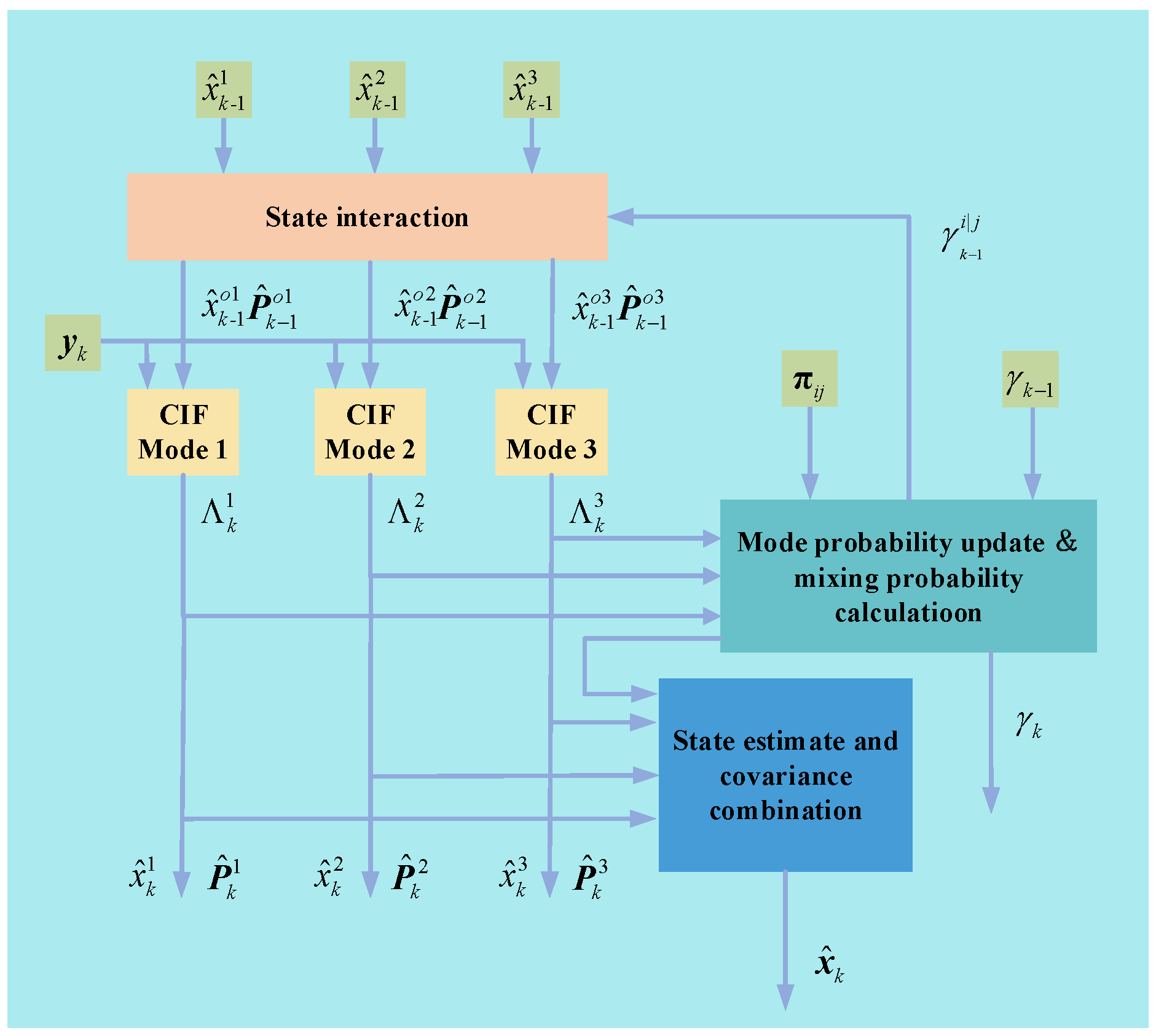
2.2. IMM-CIF Method of Maneuvering Targets

IMM is an algorithm used for target tracking and estimation [7]. This algorithm employs multiple different models simultaneously during the tracking process and each model describes the motion behavior of the target. Figure 1 depicts the block diagram of the proposed tracking IMM algorithm. This algorithm employs three CIFs. The first filter incorporates the constant velocity mode to handle the straight-line motion of the target. The second filter addresses the turning motion of the target, while the last filter considers the target’s acceleration motion.

Figure 1. Multi-model filtering framework.

The workflow of the proposed IMM-CIF method is described as follows.

• Interaction of state estimation assuming

Assuming ${\widehat{\mathit{x}}}_{k-1}^i$ represents the state estimate of filter $i$ at time $k-1$, ${\gamma }_{k-1}^{i|j}$ represents the model probability update vector at time $k-1$, where $i,j=1,\dots ,r$ and $r$ denotes the index of the CIF. The outcome of the interaction involving the state estimates, ${\widehat{\mathit{x}}}_{k-1}^{oj}$, can be expressed as

$${\widehat{\mathit{x}}}_{k-1}^{oj}={\displaystyle \sum _{i=1}^r{\widehat{\mathit{x}}}_{k-1}^i}{\gamma }_{k-1}^{i|j} i,j=1,\dots ,r$$

(8)

The corresponding state covariance matrix ${\widehat{\mathit{P}}}_{k-1}^{oj}$ can be represented as [12]

$${\widehat{\mathit{P}}}_{k-1}^{oj}={\displaystyle \sum _{i=1}^r{\gamma }_{k-1}^{i|j}}[{\widehat{\mathit{P}}}_{k-1}^j+[{\widehat{\mathit{x}}}_{k-1}^i-{\widehat{\mathit{x}}}_{k-1}^{oj}]{[{\widehat{\mathit{x}}}_{k-1}^i-{\widehat{\mathit{x}}}_{k-1}^{oj}]}^{\prime }] i,j=1,\dots ,r$$

(9)

In this step, the mixing probabilities ${\gamma }_{k-1}^{i|j}$ are calculated by mixing the previous state estimates and their covariance matrices.

$${\gamma }_{k-1}^{i|j}=\frac{1}{{\overline{e}}^j}{\pi }_{ij}{\gamma }_{k-1}^i i,j=1,\dots ,r$$

(10)

where ${\pi }_{ij}$ represents the transition probability from model $i$ to model $j$, and can be expressed as

$${\pi }_{ij}=\left[\begin{array}{cccc}{\pi }_{11}& {\pi }_{12}& \dots & {\pi }_{1r}\\ {\pi }_{21}& {\pi }_{22}& \dots & {\pi }_{2r}\\ ⋮& ⋮& \ddots & ⋮\\ {\pi }_{r1}& {\pi }_{r2}& \dots & {\pi }_{rr}\end{array}\right]$$

(11)

Moreover, the normalization constant is

$${\overline{e}}^j={\displaystyle \sum _{i=1}^r{\pi }_{ij}{\gamma }_{k-1}^i} i,j=1,\dots ,r$$

(12)

• Model update

Each CIF filter uses its input state ${\widehat{\mathit{x}}}_{k-1}^{oj}$ and error covariance matrix ${\widehat{\mathit{P}}}_{k-1}^{oj}$, together with the measurement ${\mathit{y}}_k$, to calculate its output state ${\widehat{\mathit{x}}}_k^j$ and error covariance matrix ${\widehat{\mathit{P}}}_k^j$. Moreover, both the filter residuals ${\mathit{\beta }}_k^j$ and its error covariance matrix ${\mathit{S}}_k^j$ [17] are used to calculate the likelihood of each filter, which is given by

$${\Lambda }_k^j=\frac{1}{\sqrt{2\pi {\mathit{S}}_k^j}}\exp [-0.5{({\mathit{\beta }}_k^j)}^{\prime }({\mathit{S}}_k^j)({\mathit{\beta }}_k^j)], j=1,\dots ,r$$

(13)

Then, the mode probability update for the $j$th filter is computed as

$${\gamma }_k^j=\frac{1}{G}{\Lambda }_k^j{\overline{e}}^j, j=1,\dots ,r$$

(14)

where

$$G={\displaystyle \sum _{j=1}^r{\Lambda }_k^j}{\overline{e}}^j$$

(15)

• Model output

Finally, all the filter outputs, including their state estimates ${\widehat{\mathit{x}}}_k$ and error covariance matrices ${\widehat{\mathit{P}}}_k$, are weighted and fused using the updated mode probabilities. This process ultimately produces the output state estimate and its error covariance matrix.

$${\widehat{\mathit{x}}}_k={\displaystyle \sum _{j=1}^r{\widehat{\mathit{x}}}_k^j{\gamma }_k^j}$$

(16)

$${\widehat{\mathit{P}}}_k={\displaystyle \sum _{j=1}^r{\gamma }_k^j[{\widehat{\mathit{P}}}_k^j+[{\widehat{\mathit{x}}}_k^j-{\widehat{\mathit{x}}}_k]{[{\widehat{\mathit{x}}}_k^j-{\widehat{\mathit{x}}}_k]}^{\prime }]}$$

(17)

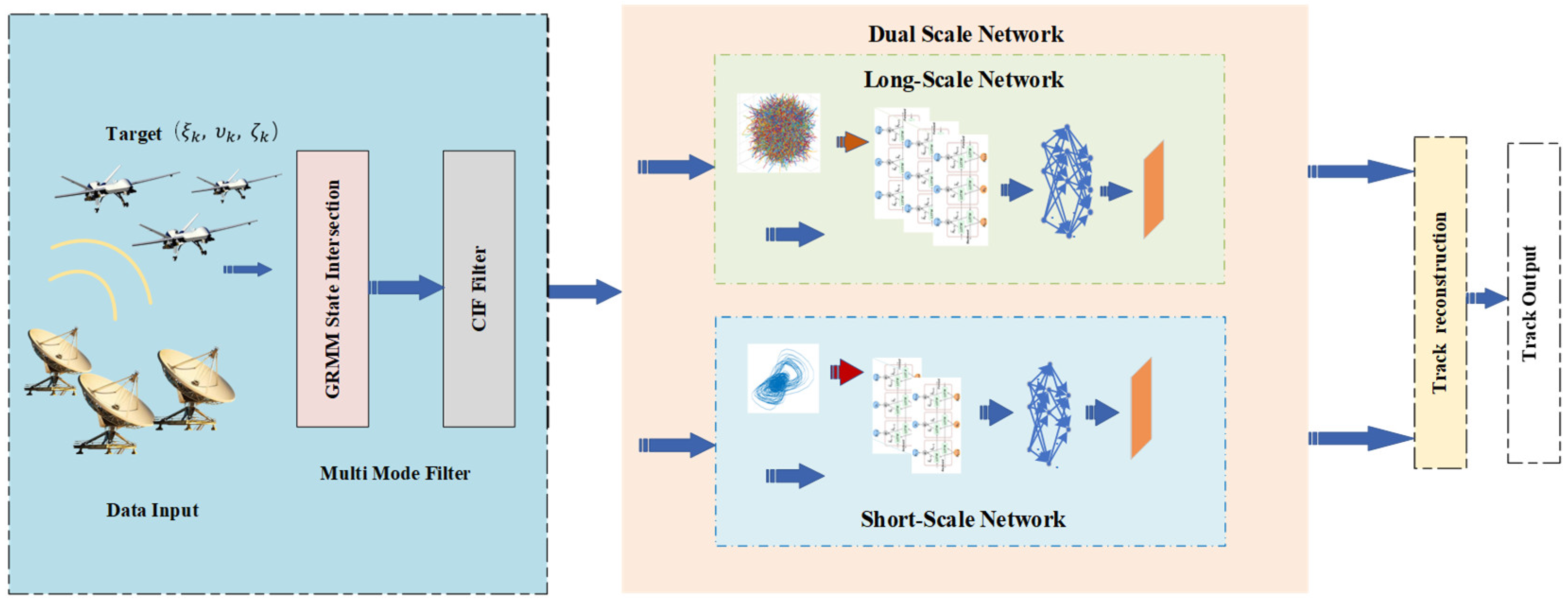
3. Proposed Tracking Method

In this section, we introduce a UAV trajectory prediction approach that relies on GRMM-CIF and DS-Bi-LSTM. We will provide details and steps related to the implementation of this technique. The sequence prediction capability of LSTM and the multi-model switching capability of IMM are used to adapt to the change of the target in different motion modes. The relevant flowchart is shown in the Figure 2 below. The data input module imports measurements acquired from radar detection of the target while initializing the state and parameters. The multi-model discrimination module employs an interactive GRMM multi-model structure to compute the model probabilities associated with the measurements. The CIF filter processing involves filtering and tracking the measurements of targets by using the GRMM-CIF framework, facilitating the estimation of the motion state. The target’s state is updated based on the outputs generated by the GRMM-CIF filter. Subsequently, the filtering state correction is conducted, and the DS-Bi-LSTM network is designed to predict the target’s state using dual scales, effectively rectifying the delay issues encountered during the tracking of multiple motion models. This entire process is iteratively executed, ensuring the continuous update of the target’s state and predictions.

Figure 2. Diagram of multi-model maneuvering target tracking based on dual-scale deep learning.

3.1. Based on GRMM-CIF Maneuvering Target Multi-Model Tracking

The proposed GRMM algorithm utilizes a neural network to calculate the Markov transition probabilities of multiple models. In this study, the method for updating the Markov chain probabilities involves using a generalized regression neural network (GRNN) [31]. GRNN is a type of neural network-based non-parametric model for estimating conditional probabilities between observed data and target models, thereby providing more accurate Markov chain probabilities. By iteratively observing and updating the probabilities, and then constructing an interactive multiple model, it becomes possible to dynamically estimate the target’s motion model and adaptively adjust it based on the observed data during the tracking process.

To implement this model, first, a Markov chain needs to be constructed. The IMM algorithm uses several different models to describe the target’s motion behavior, and each model corresponds to a state of the Markov chain. Initially, an initial Markov chain is defined, where each state corresponds to a model. Let the target state be $x$, and there are $l$ modes in the IMM (assumed to be $M^1$, $M^2$,…, $M^l$). Suppose the target state predicted by the LSTM model is ${\widehat{x}}_{k-1}$. Each mode has its own state transition probability matrix $\mathit{A}$ and observation probability matrix $\mathit{C}$. First, GRMM obtains the predicted weights by calculating the state transition probability and observation probability of each model. The weight of each model at the current moment is represented as $w_k$, and it can be calculated by the following formula:

$$w_k=P(\widehat{x}|x,M^l)·P(x|M^l)$$

(18)

where $P(\widehat{x}|x,M^l)$ is the probability of the predicted value of the neural network model under the given target state and model, and $P(x|M^l)$ is the probability of the target state under the model.

Next, the weights of each model are multiplied by their corresponding state transition probabilities to obtain a weighted state transition probability matrix $\mathit{A}(w_k)$

$$\mathit{A}(w_k)=w_k·{\mathit{A}}_k$$

(19)

Then, the weighted state transition probability matrices are combined according to certain rules, such as simple summation or weighted average, to obtain the final state transition probability matrix $\mathit{A}\prime$

$$\mathit{A}\prime ={\displaystyle \sum \mathit{A}(w_k)}$$

(20)

Finally, the state transition probability matrix $\mathit{A}\prime$ is multiplied by the observation probability matrix $\mathit{C}$ to obtain the final target state prediction:

$$\widehat{\mathit{x}}=\mathit{A}\prime ·\mathit{C}$$

(21)

3.2. Dual-Scale Bi-LSTM Tracjectory Prediction Method

Dual-scale maneuvering target trajectory prediction aims to predict the target’s trajectory by combining historical data and real-time noise-containing measurement data. The historical data are used to model the target motion, while the real-time noise-containing measurements provide information to correct the prediction results.

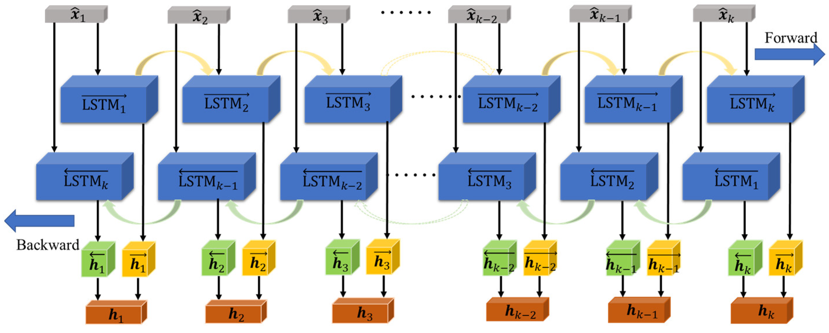
3.2.1. Bidirectional Gated Recurrent Unit

Fa Ger et al. [32] proposed a LSTM network, which enables the network to handle long-term correlations between data by introducing cell states and a series of “memory forgetting” mechanisms. LSTM establishes a long-term information retention channel through the gate structure, which can effectively retain and extract long-term information. The structure diagram of the LSTM neural network is shown in Figure 3.

Figure 3. Architecture of the LSTM layer.

LSTM is a variant of recurrent neural networks (RNNs) used for processing sequential data. Below are the formulas that describe the computation process of an LSTM cell,

$$\begin{array}{l}\mathit{i}\left(k)=\sigma \right({\mathit{W}}_{xi}{\widehat{\mathit{x}}}_k+{\mathit{W}}_{hi}{\mathit{h}}_{k-1}+{\mathit{b}}_i)\\ \mathit{f}\left(k)=\sigma \right({\mathit{W}}_{xf}{\widehat{\mathit{x}}}_k+{\mathit{W}}_{hf}{\mathit{h}}_{k-1}+{\mathit{b}}_f)\\ \mathit{a}\left(k)=\sigma \right({\mathit{W}}_{xa}{\widehat{\mathit{x}}}_k+{\mathit{W}}_{ha}{\mathit{h}}_{k-1}+{\mathit{b}}_a)\\ \mathit{o}\left(k)=\sigma \right({\mathit{W}}_{xo}{\widehat{\mathit{x}}}_k+{\mathit{W}}_{ho}{\mathit{h}}_{k-1}+{\mathit{b}}_o)\end{array}$$

(22)

where $\mathit{i}\left(k\right)$, $\mathit{f}\left(k\right)$, $\mathit{a}\left(k\right)$, and $\mathit{o}\left(k\right)$ represent input gate, forgetting gate, feature extraction, and output gate, respectively. ${\widehat{\mathit{x}}}_k$ is represented as the input at moment $k$ and ${\mathit{h}}_{k-1}$ is the hidden state value of the $k-1$ moment. ${\mathit{W}}_{xi}$, ${\mathit{W}}_{hi}$, ${\mathit{W}}_{xf}$, ${\mathit{W}}_{hf}$, ${\mathit{W}}_{xa}$, ${\mathit{W}}_{ha}$, ${\mathit{W}}_{xo}$, ${\mathit{W}}_{ho}$, ${\mathit{b}}_i$, ${\mathit{b}}_f$, ${\mathit{b}}_a$, and ${\mathit{b}}_o$ are the corresponding weight matrix and bias vector, respectively. The activation functions employed in the neural networks at different scales are distinct; however, within the same LSTM layer, the activation function remains consistent.

Bi-LSTM is a variant of the LSTM neural network architecture, comprising two LSTM subnetworks: one that processes data in a forward manner and another that processes it in a backward manner. The forward LSTM processes the input sequence in the regular order, while the backward LSTM processes it in reverse. The Bi-LSTM structure, as shown in Figure 4, is designed to capture the temporal correlation information of the feature matrix of maneuverable targets at each time step. The proposed dual-scale network integrates different Bi-LSTM layers depending on the training scale used. The output vector ${\mathit{h}}_k$ corresponding to the $k$th time point of the $i$th Bi-LSTM is the element-wise sum of the forward $\overrightarrow{{\mathit{h}}_k}$ and backward $\overleftarrow{{\mathit{h}}_k}$ LSTM outputs, and is calculated as follows:

$${\mathit{h}}_k=\overrightarrow{{\mathit{h}}_k}\oplus \overleftarrow{{\mathit{h}}_k}$$

(23)

Figure 4. Architecture of the Bi-LSTM layer.

The nonlinear activation function sigmoid can be expressed as

$${\sigma }_{\tanh }(s)=\frac{1-e^{-2s}}{1+e^{-2s}}$$

(24)

where tanh stands for the tangent hyperbolic function and s is denoted as the argument of the function. Since short-scale networks may not face severe gradient disappearance problems, simpler activation functions such as LeakyReLU can be chosen, which is faster to compute and may be a suitable choice for short-scale networks, that is:

$${\sigma }_{\mathrm{LeakyReLU}}(s)=\left\{\begin{array}{c}s , s>0\\ \alpha s , s\le 0 \end{array}\right.$$

(25)

where $\alpha$ represents the leakage rate in Leaky ReLU, and it is typically chosen to be 0.01. The optimizer chosen in this paper is the adaptive moment estimation (Adam) [33], which combines ideas from other optimization algorithms, Adagrad and RMSprop, to achieve good performance across a wide range of optimization problems. Dual-scale neural networks are optimized using the Adam optimizer to update the weight parameters of the model, minimize the prediction error, and improve the model’s predictive performance.

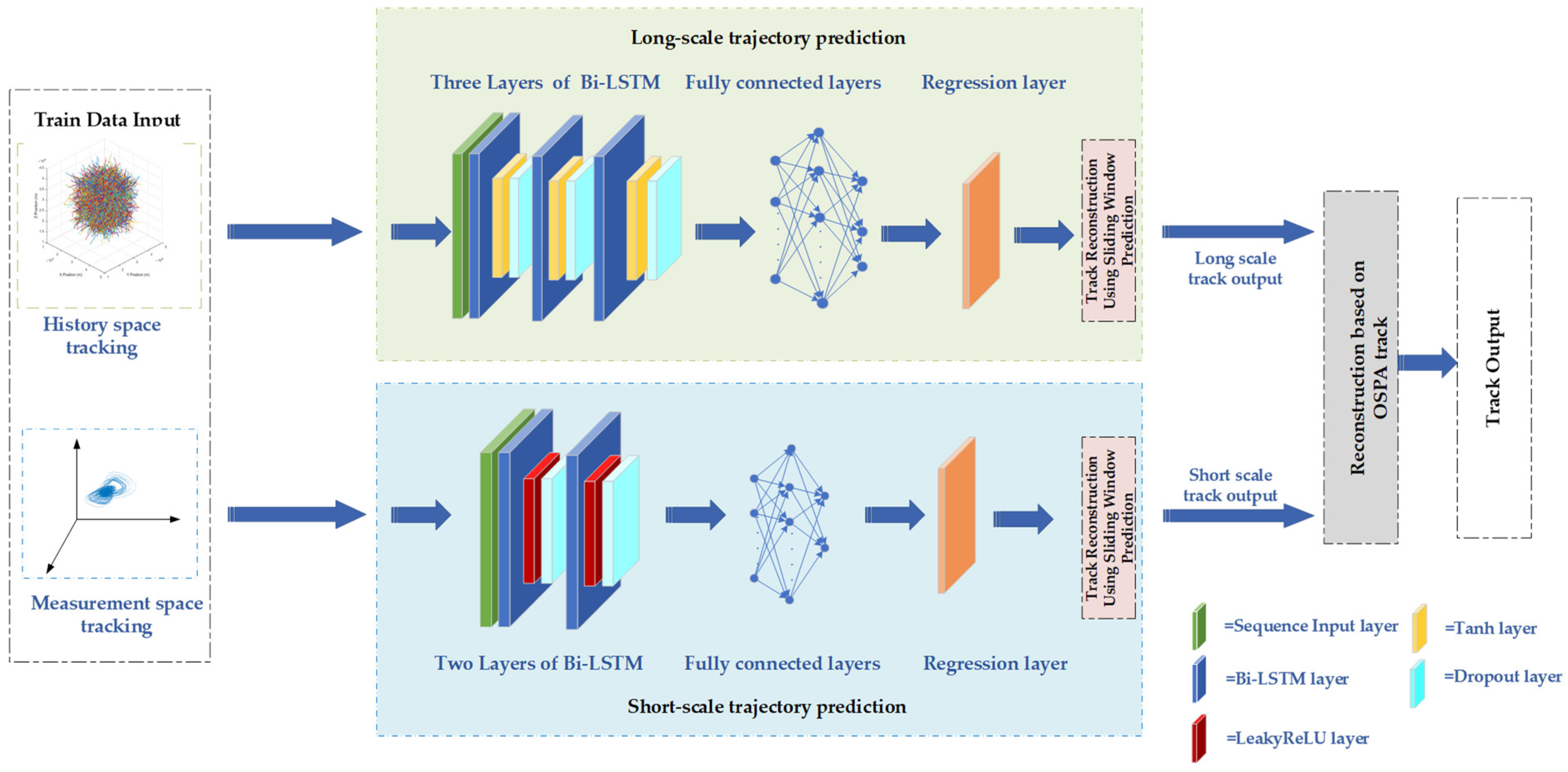
3.2.2. Neural Network Structure for Maneuvering Target Trajectory Prediction

Maneuvering target tracking based on deep learning usually requires a large amount of data for training and optimization, but due to the irregular motion trajectory of the maneuvering target, the data in the track library does not completely cover the motion state of all the maneuvering targets. Therefore, the trajectory prediction state can easily deviate from the real trajectory when dealing with the long-range maneuvering target prediction problem.

Long Scale (long-distance prediction): long-term training, more prediction points, the advantage is that the overall prediction of the track is more accurate.

Short Scale (short-distance prediction): the number of prediction points is small, the speed of prediction is fast, and the advantage is that it can assist in determining the trajectory motion state in real time.

The accuracy of trajectory prediction is improved by quickly identifying changes in the maneuvering target state. To achieve this goal, a dual-scale track prediction network is designed, as shown in Figure 5. The input data consist of tracking measurements. For the long-scale network, a three-layer Bi-LSTM network structure is designed and trained for long-distance prediction. To prevent overfitting, a tanh activation layer and a dropout layer are added after each layer of the Bi-LSTM network. For the short-scale network, the number of Bi-LSTM layers is reduced, enabling faster response in short-distance prediction. The predicted values from both the long scale and short scale are used to reconstruct output tracks, resulting in new predicted tracks with higher accuracy.

Figure 5. Neural network structure for maneuvering target trajectory prediction.

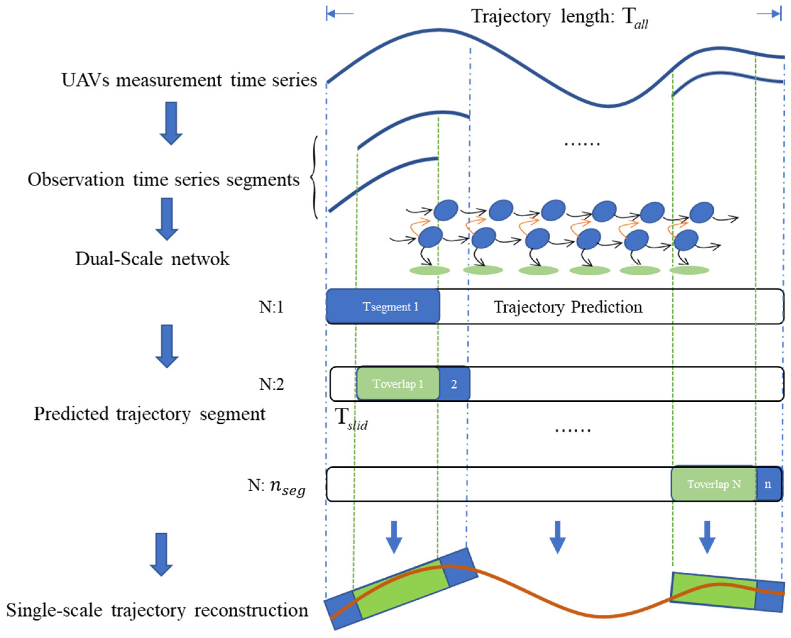
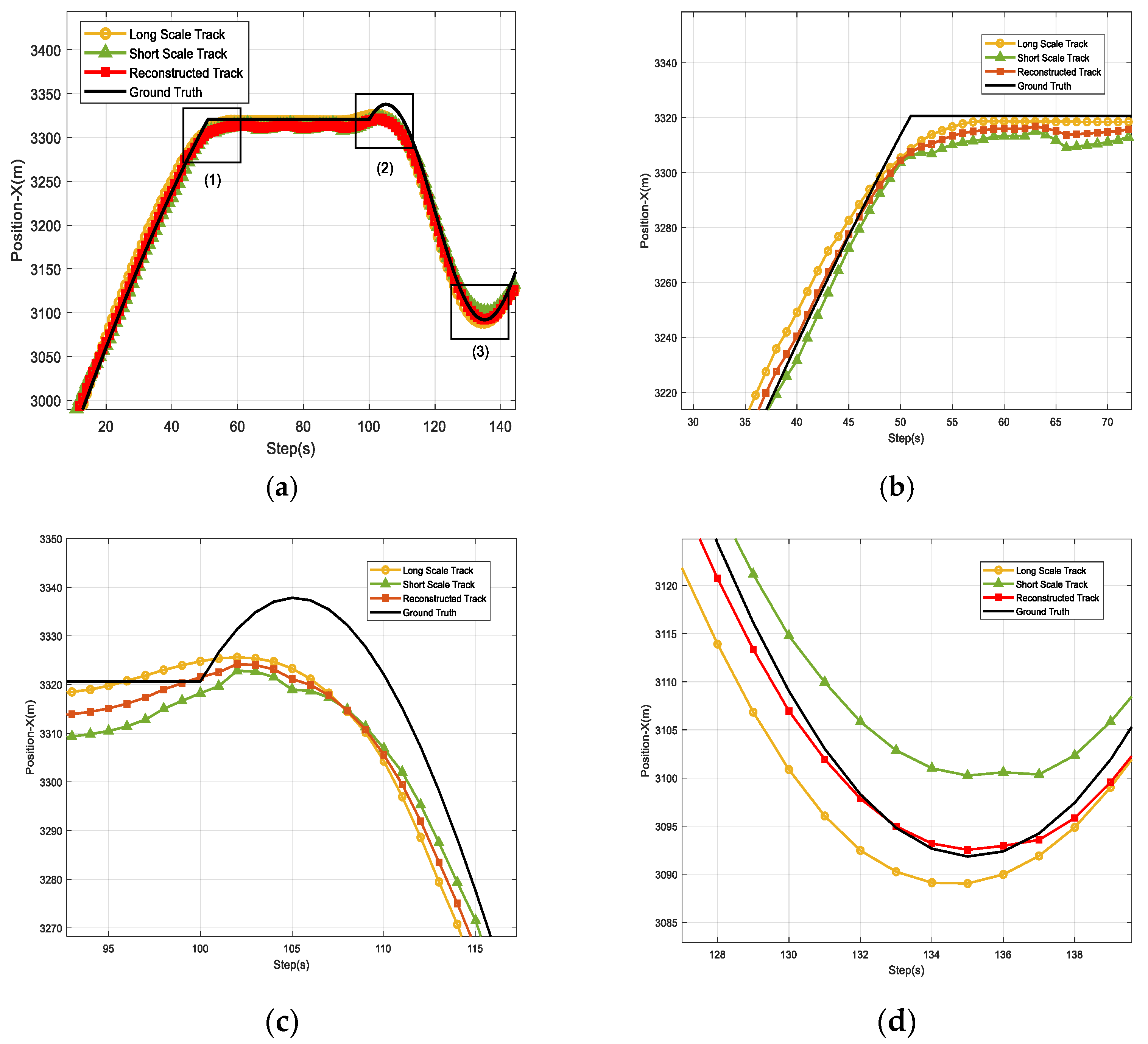
3.3. Trajectory Reconstruction

3.3.1. Sliding Window Prediction Track Reconstruction

The prediction of an entire sequence of trajectories has the potential to accumulate prediction errors, thereby potentially diminishing the model’s performance. To reduce this effect, a “moving window” approach is used in this paper [23]. We define sliding window parameters as follows, the segment size is the trajectory duration ${\mathrm{T}}_{all}$ representing the temporal length of each target’s trajectory segment, the overlap size is the temporal overlap ${\mathrm{T}}_{overloap}$ between trajectory segments ${\mathrm{T}}_{segment}$, and the num segments $n_{seg}$ is the total number of sliding trajectory segments. These parameters can be configured based on the motion characteristics of the target and the data acquisition frequency. The model is used to predict the output sequence at each time step, and the predicted output sequence is moved forward one time step in order to predict the output sequence at the next time step. The overlapping regions ${\tilde{x}}_{n_{{}_{start}}: n_{overlope}}^i$ are combined with the average of the currently predicted overlapping regions ${\tilde{x}}_{n_{{}_{overlope}}: n_{seg}}^i$ to reduce prediction error. This approach reduces the accumulation error and improves the performance of the model. Figure 6 shows the single-scale track sliding window prediction reconstruction.

Figure 6. Single-scale track sliding window prediction reconstruction.

The sliding window size setting is a key problem when motion state changes. Sliding window size ${\mathrm{T}}_{slid}$ refers to the length of window used for analysis in time series data. With a sliding window, we can analyze and process continuous data. Time scale of target transition: the sliding window size should match the time scale of the target state transition. If the target state transitions quickly, the sliding window can be chosen to have a shorter length to capture these rapid changes. On the other hand, if the target state changes slowly, we can choose a longer sliding window to smooth the data and capture the long-term trend.

3.3.2. Dual-Scale Predictive Track Reconstruction Based on OSPA

Optimal Subpattern Matching Distance (OSPA): a distance metric based on the Hungarian algorithm that can measure the overall deviation and local deviation between two tracks [34]. Compared to Euclidean and Hausdorff distances, OSPA distance is more robust and scalable.

According to 3.3.1, the trajectories reconstructed after long and short-term predictions using a single-scale sliding window are long-scale prediction reconstruction $tra{j}^1(\widehat{p})=[{\widehat{p}}_1^1,{\widehat{p}}_2^1,\dots ,{\widehat{p}}_u^1]$ and short-scale prediction reconstruction $tra{j}^2(\widehat{p})=[{\widehat{p}}_1^2,{\widehat{p}}_2^2,\dots ,{\widehat{p}}_v^2]$, the ground-truth track is $traj(p)=[p_1,p_2,\dots ,p_g]$.

The Munkres algorithm [35] is used to find the best match between tracks

$$M=(u_1^{1,2},v_1),(u_2^{1,2},v_2),\dots ,(u_k^{1,2},v_k)$$

(26)

where $u_k^{1,2}\in 1,2,\dots ,n_{\widehat{p}}$, $v_k\in 1,2,\dots ,m_p$, and $k\le \min (n_{\widehat{p}},m_p)$; $(u_k^{1,2},v_k)$ indicates that two tracks with different prediction scales match the first and middle points in the ground-truth track; and $n_{\widehat{p}}$ and $m_p$, respectively, represent the number of data points in the two tracks. Set ${\delta }_{i,j}$ to the dual-scale prediction of the distance between the first point $u_k^{1,2}$ in the track and the point $v_k$ in the ground-truth track, that is, ${\delta }_{i,j}^{1,2}=d({\widehat{p}}_i^{1,2},p_j)$.

OSPA distance can be used to determine whether the middle segment of two tracks predicted by a dual-scale neural network deviates. Assuming that the set of predicted values for the middle segment of the dual-scale track is $\widehat{p}$ and the set of values for the middle segment of the ground-truth track is $p$, the OSPA distance calculation formula is:

$$OSP{A}_c(\widehat{p},p)=\underset{\chi \in {\Pi }_c}{\min }\sqrt{\frac{1}{N}{\displaystyle \sum _{i=1}^N{‖{\widehat{p}}_i-p_{\chi }{}_{(i)}‖}^2+c(N-card(\chi ))}}$$

(27)

where ${\Pi }_c$ represents all assignment schemes; $N$ indicates the number of time steps in the middle period; ${\widehat{p}}_i$ and $p_{\chi }{}_{(i)}$ represent the predicted value of the dual-scale prediction at the $i$ time step, respectively; $c$ is the matching cost coefficient, which is used to weigh the number of assigned elements and the distance between them; and $\mathrm{card}(\chi )$ represents the number of elements assigned $\chi$ in the assignment scheme.

Calculate the dual-scale track error with the filter measurements.

$${\Delta }_{q,c}(\widehat{p},p)={\left[\frac{1}{\min (\widehat{p},p)}\left({\displaystyle \sum _{(i,j)\in M}OSP{A}_c{(tra{j}_{i_1,i_2}^{1,2},tra{j}_j)}^q}+c(\widehat{p}+p-2k)\right)\right]}^{1/q}$$

(28)

Track deviations ${\Delta }_{q,c}(\widehat{p},p)$ are based on track deviations by comparing the value of the track error with the set $\epsilon$ threshold size.

If $|{\Delta }_{q,c}(\widehat{p},p)|\le \epsilon$ is judged that the state of movement is normal, select the nearest Euclidean distance scale track segment by timestamps

If $|{\Delta }_{q,c}(\widehat{p},p)|>\epsilon$ is judged that the state of movement is deviated, select the long and short inter-scale means according to timestamps.

Finally the selected track segments are reconstructed according to timestamps.

4. System Implementation and Performance Analysis

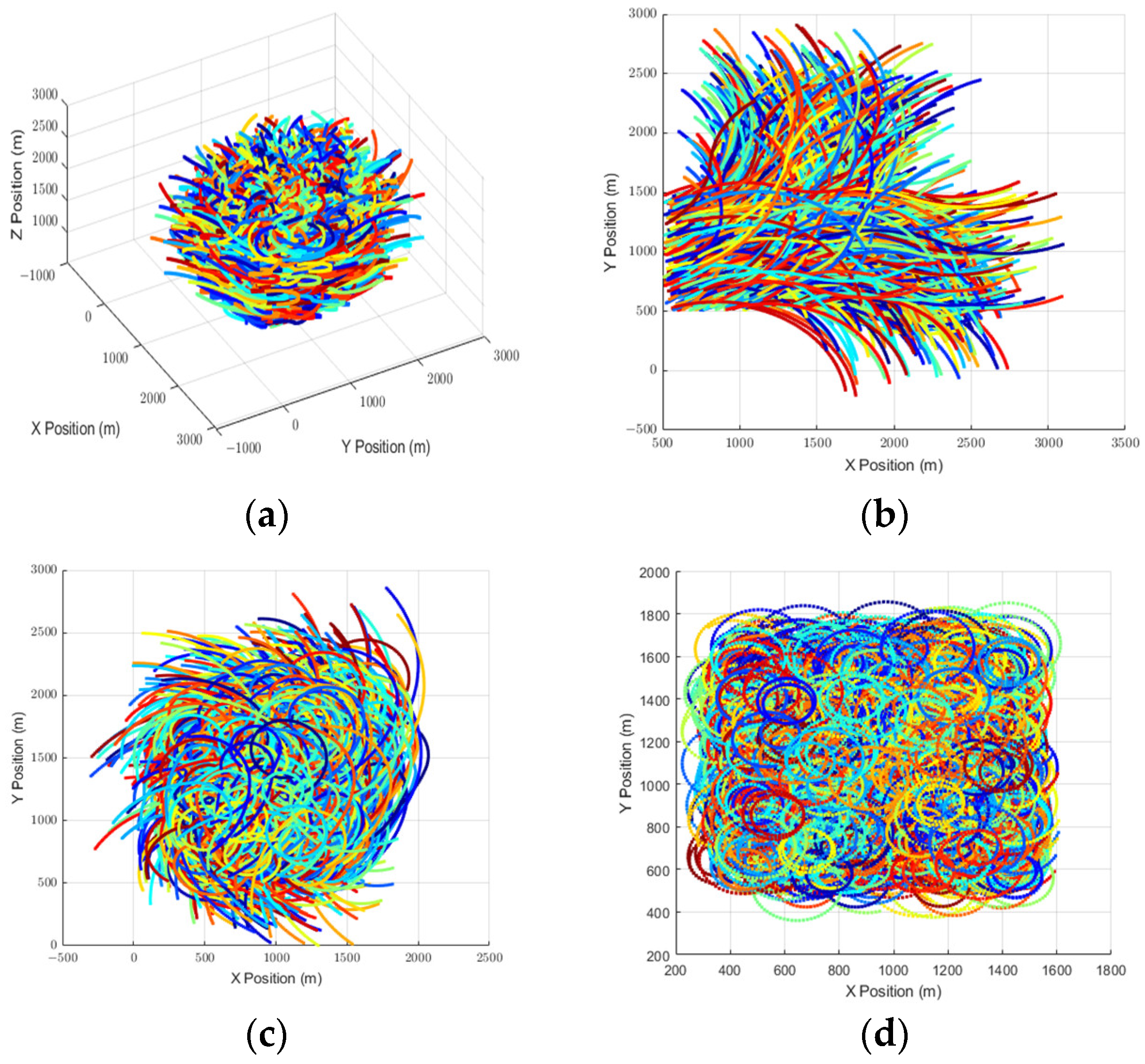
4.1. Generation of Trajectory Database

The idea of generating maneuvering target trajectory databases has been proposed in [20,22], and it has been applied to 3D coordinate systems for maneuvering target tracking. Based on the uniform motion model in (3), the acceleration model in (4), and the turning model in (5), corresponding model datasets are generated. To facilitate performance testing [36,37]. Each model’s trajectory tracking duration is 50 s with three maneuvers, resulting in a 150 s trajectory database. It is assumed that multiple maneuvering target trajectories are separable. The maneuvering target trajectory is a set of parameters that define the motion of the target in 3D space. The corresponding parameter settings are summarized in Table 1. In the table, “Length of trajectory” represents the duration of a single maneuver trajectory segment. “Initial position ([${\xi }_k, {\upsilon }_k, {\zeta }_k$] m)” indicates the initial position of the UAV in Cartesian coordinates within the radar detection range. The distances along the X, Y, and Z axes are selected within the detection range of (300, 1500) meters. “Initial velocity” represents the initial speed of the UAV, with the X, Y, and Z velocity components chosen within the range of (1, 20) m/s. The trajectory database of each model is sampled with 30,000 sets of trajectory data, where 24,000 sets are used as the training set and 6000 sets are used as the test set, to evaluate the model’s performance.

Table 1. UAV trajectory databases set parameters.

Parameters Name	Value
Length of trajectory (s)	50
Sampling time interval (s)	1
Initial position ([${\xi }_k, {\upsilon }_k, {\zeta }_k$] m)	Random (300, 1500)
Initial velocity ([${\dot{\xi }}_k, {\dot{\upsilon }}_k, {\dot{\zeta }}_k$] m/s)	Random (1, 20)
Initial acceleration velocity ([${\ddot{\xi }}_k, {\ddot{\upsilon }}_k, {\ddot{\zeta }}_k$] m2/s)	Random (1, 10)
Initial angular velocity ([${\omega }_m$] °/s)	Random (−10,10)

These parameters describe the initial state of the maneuvering target and can be used to generate a set of trajectories for the target over a specified time period. Figure 7a displays ten thousand generated trajectories of maneuvering targets within the CT mode history database. Fast-turn trajectory set, medium-turn trajectory set, slow-turn trajectory set: these refer to different sets of trajectories based on the proportion of turns executed by maneuvering targets. Each set may contain trajectories with different turn sizes (fast, medium, and slow) to represent different flight scenarios, as shown in Figure 7b–d.

Figure 7. History trajectories database (CT mode). (a) The trajectories are presented in 3D space. (b) Fast-turn trajectory set ${\omega }_1=\pm (0,1)$ °/s. (c) Medium-turn trajectory set ${\omega }_2=\pm (1,5)$ °/s. (d) Slow-turn trajectory set ${\omega }_3=\pm (5,10)$ °/s.

4.2. Preprocessing of Trajectory Data

For each maneuvering model, 30,000 trajectories were simulated, and three independent training datasets and three test datasets were created. For each training data set, we selected 80% of the trajectory randomly to train the proposed model and used the rest as a validation set. Dimensionlessness is necessary because different dimensions of the trajectories may have different units. Therefore, before implementation in the method, all the trajectory data are normalized using the min-max scaling as follows:

$$tra{j}_{\mathrm{norm}}=\frac{traj-tra{j}_{\min }}{tra{j}_{\max }-tra{j}_{\min }}\left\{\begin{array}{c}tra{j}_{\min }=\min ({\xi }_k, {\upsilon }_k, {\zeta }_k)\\ tra{j}_{\max }=\max ({\xi }_k, {\upsilon }_k, {\zeta }_k)\end{array}\right.$$

(29)

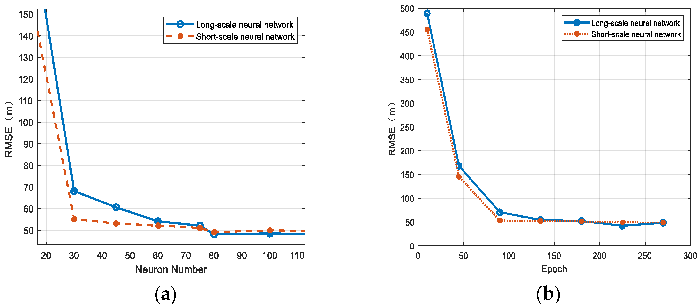
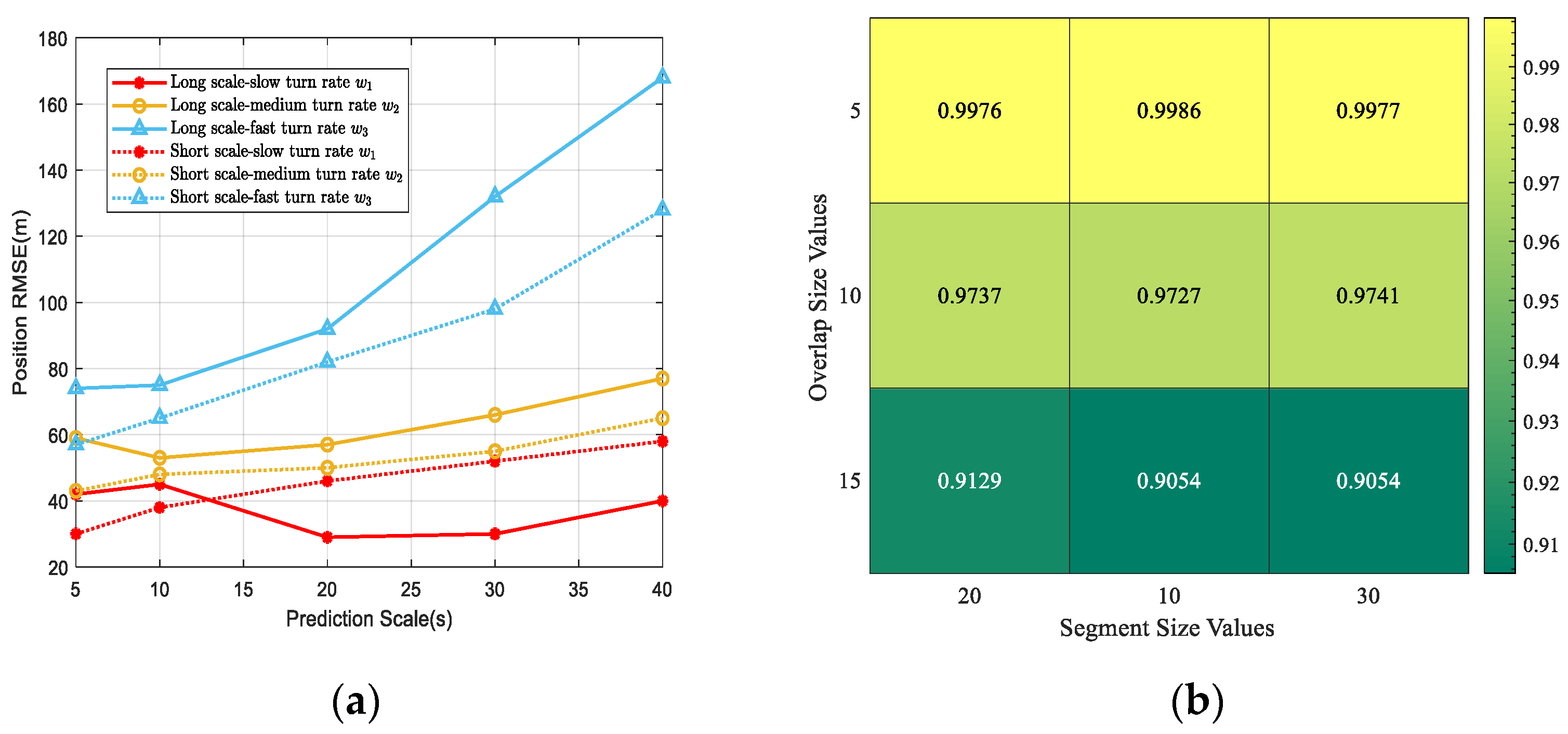
4.3. Neural Network Parameter Setting and Performance Analysis

The DS-Bi-LSTM track prediction network is a deep learning model for processing track data with stronger spatiotemporal modeling capability and higher prediction accuracy. The initial learning rate is a hyperparameter that controls the step size for parameter updating each time. Setting the initial learning rate is usually associated with a specific problem and data set. For larger datasets, a larger initial learning rate is typically chosen for faster parameter updates. A large learning rate can improve the convergence speed and quickly explore the parameter space at the beginning of training, so we design the network at the long scale to have a large initial learning probability of 0.01 and the initial learning probability of the short scale of 0.001 due to the small training set.

In dual-scale neural networks, the number of neurons can impact the prediction performance. The number of neurons represents the complexity of the network. Larger numbers of neurons generally allow the network to have higher capacity and expressive power, enabling better fitting of larger and more complex training datasets. However, using too many neurons can result in several problems. It can increase training time, computational resources, and the risk of overfitting, thereby reducing prediction performance. It can be seen from Figure 8a that the number of neurons in the dual-scale network is set to 70 and 30, respectively. Epoch is also a crucial parameter in training neural networks, and increasing the number of epochs may potentially enhance the model’s performance on the training data, as it provides the model with more opportunities to learn data features. However, if too many epochs are utilized, the model may start overfitting, leading to a decline in performance on the test data. According to Figure 8b, 75 epochs are selected for the short scale, while 225 epochs are chosen for the long scale.

Figure 8. The influence of different parameters on dual-scale neural networks. (a) Number of hidden units in the Bi-LSTM layer. (b) Epoch.

Table 2 shows the parameters of the DS-Bi-LSTM trajectory prediction network for long scale/short scale, respectively. To realize the training of track measurement values for different scales, the structural parameters of each scale network need to be adjusted accordingly. The purpose of short scale is to train quickly according to the abnormal prediction data and to detect the state transitions timely, so the parameter settings are suggested in Table 2.

Table 2. Dual-scale multi-layer Bi-LSTM trajectory prediction network parameters.

Parameter Name	Long-Scale Network	Short-Scale Network
Batch size	25	10
Initial learning rate	0.01	0.001
Epoch	225	75
Dropout layer	0.02	0.02
Hidden unit numbers of the Bi-LSTM layer	70	30
Time series step size	15	3

Table 3 shows the mean absolute percentage error (MAPE), mean absolute error (MAE), mean squared error (MSE), root mean squared error (RMSE), and the coefficient of determination (R-value) for different configurations of Bi-LSTM layers in the long-scale network. When the number of Bi-LSTM layers is increased from one to two, the network’s output accuracy significantly improves. This means that adding an additional Bi-LSTM layer helps the network capture more complex patterns and features in the data, leading to better predictions. When the number of layers is further increased to three, the R-value is the largest. The R-value measures how well the predictions fit the actual data. A higher R-value indicates that the network fits the data better and has a stronger predictive power. However, when the number of layers is increased to four, the network becomes too complex and overfitting occurs. Overfitting happens when the model becomes too specialized in the training data and performs poorly on unseen data, such as the validation or test set. In this case, the prediction effect is reduced because the model is not able to generalize well to new data. Based on these observations, we set the number of Bi-LSTM layers to three. This choice strikes a balance between increasing model complexity to capture more patterns and avoiding overfitting.

Table 3. Performance of network structure with different numbers of layers for trajectory prediction.

Evaluation Indicators	Bi-LSTM Network Structure
	One Layer	Two Layers	Three Layers	Four Layers
MAPE	−0.08	−0.05	−0.02	−0.02
MAE	12.441	7.858	3.407	4.007
MSE	1679.470	786.183	168.645	262.039
RMSE	12.959	8.867	4.107	5.118
R	0.71	0.86	0.97	0.95

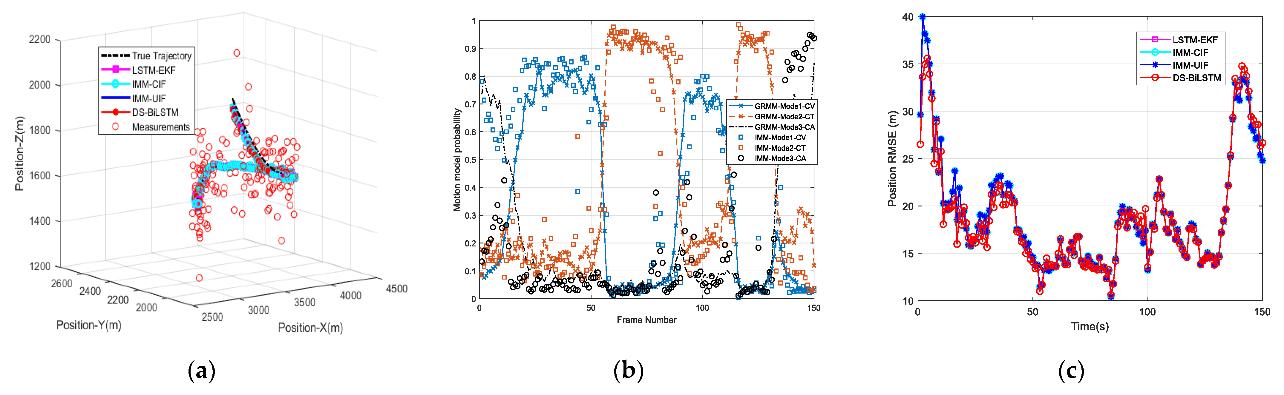
4.4. Simulation Scenario Configuration

In this part, we determine the sliding window scale of the dual-scale network according to the motion state. It is an effective method to use multi-Bi-LSTMs to predict the trajectory of maneuvering targets and consider the influence of the target motion state on the scale of sliding windows. By adaptively adjusting the scale of the sliding window, the dynamic characteristics of the target in different motion states can be better captured.

The turning size of the maneuvering target can be determined by the turning angle, which refers to the angle at which the target changes course per unit time. The larger the turning angle, the greater the angle at which the target changes course per unit time, resulting in faster turns.

After the network parameters are determined, the prediction scale of the sliding window is also an important factor. The long- and short-scale sliding window settings are related to the motion parameters. For turning (fast turn, medium turn, slow turn), we set the minimum value of the sliding window according to the RMSE performance. The position RMSEs of different motion states, plotted against the sliding window scale, are shown in Figure 9a. In the same scale, the blue line represents the maximum error for rapid turns, while the red line corresponds to the minimum error for low-speed turns. When the turning rates are the same, solid lines represent the long scale, while dashed lines represent the short scale. As the turning rate increases, the error increases for the long scale, while the short scale exhibits good tracking performance for high turning rates.

Figure 9. Scale sliding windows are set due to turning rate. (a) Dual-scale prediction performance. (b) Correlation coefficient heatmap between segment size values and overlap values.

In Figure 9b, the plot shows the segmenting values and overlapping values. The yellow heat map indicates a high correlation coefficient, while the green heat map represents a low correlation coefficient. Based on linear correlation, appropriate values for window segmentation and overlap are selected to ensure optimal windowing performance.

Scenario 2: For trajectory prediction at different scales, in order to achieve overall an performance improvement, this paper proposes OSPA threshold discrimination for trajectory reconstruction. Based on the threshold value, the short-scale and long-scale predictions are combined to reconstruct the target’s trajectory more accurately.

As the motion state of a maneuvering target changes, the real-time short-scale predictions of the trajectory state closely follow the actual trajectory. However, due to the limited size of the training dataset, short-scale predictions tend to be smoother and are more susceptible to noise interference. On the other hand, long-scale predictions exhibit better performance when the trajectory is smooth and are less affected by noise interference.

When the dual-scale track error is within the range of the OSPA calculated threshold, the network selects the trajectory that is closer to the measurement point; otherwise, the network computes the average value of the two trajectories as the reconstruction trajectory. The results are shown in Figure 10.

Figure 10. Real and reconstructed trajectories of the maneuvering target. (a) The whole reconstructed trajectory. (b) Enlarged true and predicted trajectories at position 1. (c) Enlarged true and predicted trajectories at Position 2. (d) Enlarged true and predicted trajectories at Position 3.

Table 4 shows the three target trajectory parameters. The performance advantage of the dual-scale neural network combined with GRMM is that it can improve the maneuvering target tracking performance of the uncertain model and simulate the real motion state according to the three common motion models of UAVs.

Table 4. Target trajectory parameters.

Index	Initial State	The First Part	The Second Part	The Third Part
1	[1200 m, 1400 m, 1300 m, 12 m/s, 7 m/s, 1 m/s]	50 s, CT mode, ${\overline{\mathit{\varpi }}}_1$ = 4.5 °/s	50 s, CV mode	50 s, CT mode, ${\overline{\mathit{\varpi }}}_3$ = 3.5 °/s
2	[900 m, 700 m, 1100 m, 8 m/s, 5 m/s, 1 m/s]	50 s, CT mode, ${\overline{\mathit{\varpi }}}_1$ = 4.5 °/s	50 s, CT mode, ${\overline{\mathit{\varpi }}}_2$ = 2.5 °/s	50 s, CT mode, ${\overline{\mathit{\varpi }}}_3$ = 3.5 °/s
3	[1100 m, 800 m, 500 m, 10 m/s, 6 m/s, 1 m/s]	50 s, CV mode	50 s, CT mode, ${\overline{\mathit{\varpi }}}_2$ = −4.5 °/s	50 s, CA mode, a = [6 5 3] m/s2

For different tracking algorithms, Figure 11 presents the tracking comparison results of the first maneuvering target. The tracking model of the first maneuvering target is simulated as an aircraft performing a 50 s turn, followed by a 50 s constant speed segment, and another 50 s turn. The estimated trajectories of the four algorithms of this experiment are shown in Figure 11a–d. Figure 11a–d also show the true trajectory and corresponding measurements. Then, the transition probabilities of the maneuvering target motion states of our proposed method are shown in Figure 11e. Finally, the prediction accuracy in terms of RMSE for the position of the four algorithms is shown in Figure 11f.

Figure 11. Tracking performance comparison of four algorithms for the first maneuvering target. (a) True and predicted trajectories in 3D Cartesian coordinate system. (b) True and predicted trajectories in X and Y directions. (c) True and predicted trajectories in X and Z directions. (d) True and predicted trajectories in Y and Z directions. (e) Transition probabilities of the maneuvering target motion states. (f) Position RMSE.

The tracking model of the second maneuvering target is simulated as an aircraft performing a 50 s turn, followed by a 50 s turn, and another 50 s turn. The third target performs a 50 s CV, followed by a 50 s turn, and another 50 s CA. The corresponding results of the second and third targets are shown in Figure 12 and Figure 13, respectively. From the tracking results of Figure 11, Figure 12 and Figure 13, it can be seen that the DS-BiLSTM remains precise and stable for tracking all trajectories. Obviously, in these figures, all tracking RMSEs of our DS-BiLSTM algorithm provide the highest prediction accuracy in all simulation experiments compared to the other three algorithms. Specifically, the LSTM method relies on the original historical data set, so its prediction result fluctuates greatly when the motion state changes. Moreover, the IMM algorithm requires a known priori model transfer probability, the performance is greatly reduced if no prior probability is provided. Though the IMM has the known prior model transfer probability, the tracking state sometimes can be delayed, so the tracking effect is also affected. In summary, our DS-BiLSTM algorithm outperforms the state-of-the-art LSTM and IMM algorithms for tracking maneuvering targets. We have supplemented Figure 14 to illustrate drone tracking under different durations of uncertain maneuvers, providing an in-depth analysis of our algorithm. This addition aims to offer a more comprehensive evaluation of the model’s robustness and effectiveness, particularly in addressing a broader range of scenarios with varying durations of maneuvers. Figure 11e, Figure 12, Figure 13 and Figure 14b indicate that, with the optimization of GRNN, the recognition probabilities for different motion models in GRMM have improved, surpassing traditional IMM. This enhancement contributes to the improvement of trajectory tracking performance for maneuvering targets with various motion models.

Figure 12. Tracking performance comparison of four algorithms for the second maneuvering target. (a) True and predicted trajectories in 3D Cartesian coordinate system. (b) Transition probabilities of the maneuvering target motion states. (c) Position RMSE.

Figure 13. Tracking performance comparison of four algorithms for the third maneuvering target. (a) True and predicted trajectories in 3D Cartesian coordinate system. (b) Transition probabilities of the maneuvering target motion states. (c) Position RMSE.

Figure 14. Tracking performance comparison of four algorithms for the fourth maneuvering target. (a) True and predicted trajectories in 3D Cartesian coordinate system. (b) Transition probabilities of the maneuvering target motion states. (c) Position RMSE.

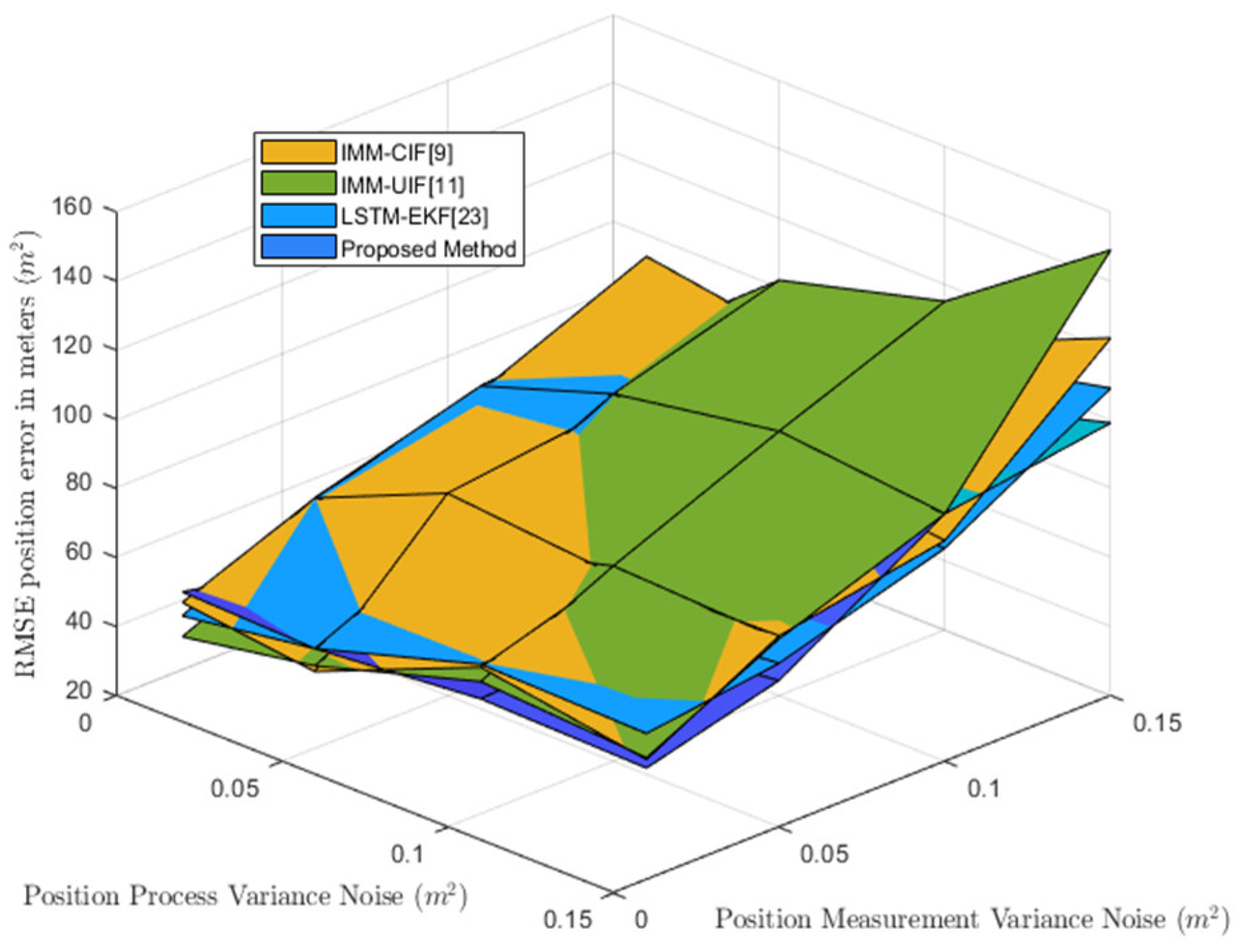
4.5. Analysis of Filtering Performance under Different Noise Conditions

To verify the robustness of the proposed dual-scale neural network in different noisy environments, we take the prediction of the movement distance of a maneuvering target as an example. We compare the tracking ability of four algorithms under different noise levels by varying the standard deviation of the position measurement noise.

We generated synthetic datasets with different noise levels by adding Gaussian noise to the ground-truth distance measurements and measured the prediction error between the estimated distance and the ground-truth distance for each algorithm under different noise conditions. Evaluation metrics RMSE was used to quantify the performance of the algorithms. As shown in Table 5 and Table 6, the experimental results show that the dual-scale neural network is robust compared to the other three algorithms, showing smaller prediction errors and better tracking ability at various noise levels.

Table 5. RMSE performance of four methods with various process noise levels (units: m²).

RMSE	Process Noise Variance Values
	0.001	0.015	0.030	0.045
IMM-CIF [9]	5.09	7.89	10.58	22.52
IMM-UIF [11]	5.43	8.27	13.87	24.05
LSTM-EKF [23]	4.24	7.23	9.32	19.07
Proposed method	4.06	5.57	8.27	14.51

Table 6. RMSE performance of four methods with various measurement noise levels (units: m).

RMSE	Measurement Noise Values
	10	20	30	40
IMM-CIF [9]	4.46	8.24	12.98	29.72
IMM-UIF [11]	5.34	8.58	14. 58	28.08
LSTM-EKF [23]	4.35	7.58	9.26	24. 45
Proposed method	3.86	6.57	10.38	18.23

These findings confirm the effectiveness of the proposed dual-scale neural network in mitigating the effects of noise and improving the accuracy of moving target motion distance prediction, as shown in Figure 15. The position RMSE of maneuvering targets increases with process and measurement noise and shows an unstable trend. The lowest region of the position RMSE of the folded plot represents that the algorithm performs better in that range under specific noise conditions. Observing the magnitude of change in the RMSE curve, the curve of the algorithm proposed in this paper may be smoother, whereas the other algorithms may be more unstable when the noise changes.

Figure 15. RMSE performance comparison of four filtering algorithms with various noise levels.

Overall, the experimental results validate the robustness of the proposed dual-scale neural network in different noise environments and highlight its potential for enhancing the accuracy and reliability of motion distance prediction in practical applications.

5. Discussion

The high maneuverability and diverse trajectory modes of UAVs bring a few challenges to object tracking. The traditional filtering model heavily relies on priori parameters and therefore degrades significantly when the priori parameters dismatch the maneuvering target motion. To overcome these challenges, we use a neural network to determine the Markovian priori transfer probability to improve the accuracy of target motion model switching, and a dual-scale neural prediction network is proposed to solve the state delay problem stored in the interacting model. The proposed method improves the tracking performance of the maneuvering target and makes it suitable for agile UAVs.

First, a historical trajectory database is generated using data-driven and machine-learning techniques. This database is then utilized for training a model that predicts the switching behavior of the model under different environments and conditions. We also tackle the temporal prediction of maneuvering targets problem, which is influenced by the state transitions. Taking turn rate as an example, we design appropriate sliding window scales based on turning rate analysis, as shown in Figure 9. The proposed dual-scale maneuvering target state prediction algorithm optimizes the problem of prediction deviation caused by training set influence observed with single-scale predictions, as shown in Figure 10. Due to their sensitivity towards such transitions, single-scale predictions tend to deteriorate when there are different motion transitions of maneuvering targets. By employing OSPA distance for judgment, our dual-scale neural network selects a more accurate scale for trajectory reconstruction, enhancing the overall tracking performance of maneuvering targets and addressing issues faced by separate long and short-scale predictions, such as prediction deviation or poor tracking performance affected by noise. Figure 11, Figure 12, Figure 13 and Figure 14 demonstrate tracking results for maneuvering targets with various motion patterns and illustrate that within the GRMM-CIF framework, our dual-scale neural network exhibits strong adaptability during target transition tracking with superior accuracy throughout the entire tracking period compared to traditional tracking algorithms. Figure 15 analyzes how different levels of process noise and measurement noise interference affect filtering when applying various algorithms to track the same maneuvering target. It is found that our proposed dual-scale neural network algorithm possesses more robust anti-interference capabilities.

Typically, process noise and measurement noise are unknown; however, in this paper, we assume that the noise is known and remains constant in order to validate the algorithm performance. In future investigations, we will consider closer to the practical detection environments, such as time-varying noise and detection target loss. Additionally, we will explore the possibility of expanding the proposed approach to multi-station UAV swarm target tracking.

6. Conclusions

To summarize the above, we present a novel hybrid-driven multi-model discrete-time system filter for tracking maneuvering targets, such as UAVs. This filter leverages the advantages of the underlying system knowledge obtained from big data and the domain-specific expertise in target dynamics. By synergistically integrating these two sources of information, we aim to enhance the accuracy and efficiency of target tracking.

The GRMM-CIF filtering architecture is established to filter and track the measured values of the target using multiple motion models, effectively addressing the challenge of modeling uncertain target motion. By avoiding data dependency in the neural network when the motion state changes, the method improves the accuracy of tracking. In trajectory reconstruction, the model can choose a sliding window of appropriate length to capture motion information. The performance advantage of the dual-scale neural network combined with GRMM is that it can improve the maneuvering target tracking performance of the uncertain model.

The DS-BiLSTM algorithm is devised to tackle the prediction delay issue arising from target state changes under multiple models. This novel algorithm facilitates swift assessment of target motion amidst variations of the motion state of maneuvering UAVs, thereby ensuring timely and precise predictions. The dual-scale network consistently outperforms the other algorithms with robustness, showing fewer prediction errors and better tracking ability at various noise levels. We confirm the effectiveness of the proposed dual-scale neural network in mitigating the effects of noise and improving the accuracy of motion distance prediction for maneuvering targets.

The results presented herein exemplify the algorithm’s exceptional performance with regard to tracking accuracy, robustness, and adaptability across varying environmental conditions. Furthermore, when compared to classical target tracking algorithms, our algorithm exhibits faster response in perceiving maneuvers and state transitions, thereby significantly reducing peak tracking errors. In future research, we might explore extending the proposed algorithm’s translation into a multi-station fusion structure to further enhance its tracking performance.

References

- Gu, J.; Su, T.; Wang, Q.; Du, X.; Guizani, M. Multiple moving targets surveillance based on a cooperative network for multi-UAV. IEEE Commun. 2018, 56, 82–89. [Google Scholar] [CrossRef]
- Tian, W.; Fang, L.; Li, W.; Ni, N.; Wang, R.; Hu, C.; Liu, H.; Luo, W. Deep-Learning-Based Multiple Model Tracking Method for Targets with Complex Maneuvering Motion. Remote Sens. 2022, 14, 3276–3299. [Google Scholar] [CrossRef]
- Roonizi, A.K. An Efficient Algorithm for Maneuvering Target Tracking [Tips & Tricks]. IEEE Signal Proc. 2021, 38, 122–130. [Google Scholar]
- Singer, R. Estimating optimal tracking filter performance for manned maneuvering targets. IEEE Trans. Aerosp. Electron. Syst. 1970, 4, 473–483. [Google Scholar] [CrossRef]
- Frencl, V.; do Val, J.B.; Mendes, R.; Zuniga, Y. Turn rate estimation using range rate measurements for fast manoeuvring tracking. IET Radar Sonar Navig. 2017, 11, 1099–1107. [Google Scholar] [CrossRef]
- Lan, H.; Ma, J.; Wang, Z.; Pan, Q.; Xu, X. A message passing approach for multiple maneuvering target tracking. Signal Process. 2020, 174, 107621. [Google Scholar] [CrossRef]
- Genovese, A. The interacting multiple model algorithm for accurate state estimation of maneuvering targets. J. Hopkins APL Tech. Dig. 2001, 22, 614–623. [Google Scholar]
- Revach, G.; Shlezinger, N.; Ni, X.; Escoriza, A.; van Sloun, R.J.; Eldar, Y. KalmanNet: Neural Network Aided Kalman Filtering for Partially Known Dynamics. IEEE Trans. Signal Process. 2022, 70, 1532–1547. [Google Scholar] [CrossRef]
- Zhang, D.; Shen, Z.; Song, Y. Robust adaptive fault-tolerant control of nonlinear uncertain systems tracking uncertain target trajectory. Inf. Sci. 2017, 415, 446–460. [Google Scholar] [CrossRef]
- Li, X.; Jilkov, V. Survey of maneuvering target tracking. Part V: Multiple-model methods. IEEE Trans. Aerosp. Electron. Syst. 2005, 41, 1255–1321. [Google Scholar]
- Munir, A.; Mirza, J. Parameter adjustment in the turn rate models in the interacting multiple model algorithm to track a maneuvering target. In Proceedings of the Twenty-First IEEE International Multi Topic Conference, Lahore, Pakistan, 30 December 2001; pp. 262–266. [Google Scholar]
- Blom, H.; Barshalom, Y. The interacting multiple model algorithm for systems with Markovian switching coefficients. IEEE Trans. Autom. Control 1988, 33, 780–783. [Google Scholar] [CrossRef]
- Youn, W.; Ko, N.; Gadsden, S.; Myung, H. A Novel Multiple-Model Adaptive Kalman Filter for an Unknown Measurement Loss Probability. IEEE Trans. Instrum. Meas. 2021, 70, 1–11. [Google Scholar] [CrossRef]
- Na, K.; Choi, S.; Kim, J. Adaptive Target Tracking with Interacting Heterogeneous Motion Models. IEEE Trans. Intell. Transp. Syst. 2022, 23, 21301–21313. [Google Scholar] [CrossRef]
- Lu, C.; Feng, W.; Li, W.; Zhang, Y.; Guo, Y. An adaptive IMM filter for jump Markov systems with inaccurate noise covariances in the presence of missing measurements. Digit. Signal Process. 2022, 127, 1–12. [Google Scholar] [CrossRef]
- He, S.; Wu, P.; Li, X.; Bo, Y.; Yun, P. Adaptive Modified Unbiased Minimum-Variance Estimation for Highly Maneuvering Target Tracking with Model Mismatch. IEEE Trans. Instrum. Meas. 2023, 72, 103529. [Google Scholar] [CrossRef]
- Eltoukhy, M.; Ahmad, M.; Swamy, M. An Adaptive Turn Rate Estimation for Tracking a Maneuvering Target. IEEE Access 2020, 8, 94176–94189. [Google Scholar] [CrossRef]
- Yun, P.; Wu, P.; He, S.; Li, X. A variational Bayesian based robust cubature Kalman filter under dynamic model mismatch and outliers interference. Measurement 2022, 191, 110063. [Google Scholar] [CrossRef]
- Zhang, J.; Xiong, J.; Lan, X.; Shen, Y.; Chen, X.; Xi, Q. Trajectory Prediction of Hypersonic Glide Vehicle Based on Empirical Wavelet Transform and Attention Convolutional Long Short-Term Memory Network. IEEE Sens. J. 2022, 22, 4601–4615. [Google Scholar] [CrossRef]
- Xiong, W.; Zhu, H.; Cui, Y. A hybrid-driven continuous-time filter for manoeuvering target tracking. IET Radar Sonar Navig. 2022, 16, 2053–2066. [Google Scholar] [CrossRef]
- Wang, C.; Zheng, J.; Jiu, B.; Liu, H. Model-and-Data-Driven Method for Radar Highly Maneuvering Target Detection. IEEE Trans. Aerosp. Electron. Syst. 2021, 57, 2201–2217. [Google Scholar] [CrossRef]
- Gao, C.; Yan, J.; Zhou, S.; Varshney, P.; Liu, H. Long short-term memory-based deep recurrent neural networks for target tracking. Inf. Sci. 2019, 502, 279–296. [Google Scholar] [CrossRef]
- Liu, J.; Wang, Z.; Xu, M. DeepMTT: A deep learning maneuvering target-tracking algorithm based on bidirectional LSTM network. Inf. Fusion 2020, 53, 289–304. [Google Scholar] [CrossRef]
- Xie, Y.; Zhuang, X.; Xi, Z.; Chen, H. Dual-Channel and Bidirectional Neural Network for Hypersonic Glide Vehicle Trajectory Prediction. IEEE Access 2021, 9, 92913–92924. [Google Scholar] [CrossRef]
- Gao, C.; Liu, H.; Zhou, S.; Su, H.; Chen, B.; Yan, J.; Yin, K. Maneuvering Target Tracking with Recurrent Neural Networks for Radar Application. In Proceedings of the 2018 International Conference on Radar (Radar), Brisbane, QLD, Australia, 27–31 August 2018; pp. 1–5. [Google Scholar]
- Li, X.; Jilkov, V. Survey of maneuvering target tracking. Part I: Dynamic models. IEEE Trans. Aerosp. Electron. Syst. 2003, 39, 1333–1364. [Google Scholar]
- Arulampalam, S.; Badriasl, L.; Ristic, B. Closed-Form Estimator for Bearings-Only Fusion of Heterogeneous Passive Sensors. IEEE Trans. Signal Process. 2020, 68, 6681–6695. [Google Scholar] [CrossRef]
- Xie, G.; Sun, L.; Wen, T.; Hei, X.; Qian, F. Adaptive Transition Probability Matrix-Based Parallel IMM Algorithm. IEEE Trans. Syst. Man Cybern. Syst. 2021, 51, 2980–2989. [Google Scholar] [CrossRef]
- Yu, W.; Yu, H.; Du, J.; Zhang, M.; Liu, J. DeepGTT: A general trajectory tracking deep learning algorithm based on dynamic law learning. IET Radar Sonar Navig. 2021, 15, 1125–1150. [Google Scholar] [CrossRef]
- Chandra, K.; Gu, D.; Postlethwaite, I. Cubature information filter and its applications. In Proceedings of the 2011 IEEE American Control Conference, San Francisco, CA, USA, 29 June–1 July 2011; pp. 3609–3614. [Google Scholar]
- Jondhale, S.; Deshpande, R. Kalman Filtering Framework-Based Real Time Target Tracking in Wireless Sensor Networks Using Generalized Regression Neural Networks. IEEE Sens. J. 2019, 19, 224–233. [Google Scholar] [CrossRef]
- Gers, F.; Schtmidhuber, J. LSTM recurrent networks learn simple context-free and context-sensitive languages. IEEE Trans. Neural Netw. 2001, 12, 1333–1340. [Google Scholar] [CrossRef]
- Kingma, D.; Ba, J. Adam: A method for stochastic optimization. Comput. Sci. 2014, 1, 1–15. [Google Scholar]
- Schuhmacher, D.; Vo, B.T.; Vo, B.N. A consistent metric for performance evaluation of multi-object filters. IEEE Trans. Signal Process. 2008, 56, 3447–3457. [Google Scholar] [CrossRef]
- Hernandez, D.; Cecilia, M.; Calafate, T. The Kuhn-Munkres algorithm for efficient vertical takeoff of UAV swarms. In Proceedings of the Ninety-Third Vehicular Technology Conference, Helsinki, Finland, 25–28 April 2021. [Google Scholar]
- Kose, O.; Oktay, T. Simultaneous design of morphing hexarotor and autopilot system by using deep neural network and SPSA. Aircr. Eng. Aerosp. Technol. 2023, 95, 939–949. [Google Scholar] [CrossRef]
- Liang, C.; Lei, L.; Chen, L. Multi-UAV autonomous collision avoidance based on PPO-GIC algorithm with CNN-LSTM fusion network. Neural Netw. 2023, 162, 21–33. [Google Scholar] [CrossRef] [PubMed]
Disclaimer/Publisher’s Note: The statements, opinions and data contained in all publications are solely those of the individual author(s) and contributor(s) and not of MDPI and/or the editor(s). MDPI and/or the editor(s) disclaim responsibility for any injury to people or property resulting from any ideas, methods, instructions or products referred to in the content. |
© 2023 by the authors. Licensee MDPI, Basel, Switzerland. This article is an open access article distributed under the terms and conditions of the Creative Commons Attribution (CC BY) license (https://creativecommons.org/licenses/by/4.0/).