Distributed Consensus-Based Tracking with Inverse Covariance Intersection in Bearing-Only UAV Networks

Highlights

What are the main findings?

• The DCE–ICI method is designed for high-accuracy passive tracking of maneuvering targets.
• With consensus iterative fusion, DCE–ICI ensures fast convergence.

What are the implications of the main finding?

• DCE–ICI enables each UAV to obtain precise and consensus estimation results within a distributed system.
• For a specific iteration error, the DCE–ICI can reduce the number of consensus iterations.

Abstract

High-precision and consensus tracking of a long-range maneuvering target presents a significant challenge for unmanned aerial vehicles (UAVs) in complex denied environments. Earlier studies rarely considered the fast convergence and fusion accuracy of distributed consensus tracking in bearing-only UAV networks. This article proposes a distributed consensus-based estimation (DCE) method with inverse covariance intersection (ICI) fusion rule in the framework of local estimation, consensus iteration, and fusion estimation. Combined with the contribution of measurements from neighboring UAVs, the local estimation of target tracking can be achieved by a square-root cubature information filter (SRCIF) in bearing-only UAVs. Based on local estimation and centralities in a multi-UAV network, each UAV platform can obtain consensus results in a finite number of iterations. Then, the fusion estimations are the consensus with the global ICI fusion rule. Furthermore, the fusion estimations are analyzed in consensus, finiteness, and boundedness. Numerical simulations are performed to validate the effectiveness and superiority of the proposed DCE–ICI method.

1. Introduction

Distributed estimation by multiple UAV networks offers several advantages over central estimation for tracking maneuvering targets, including greater scalability, better robustness, lower communication requirements, and lower computational costs [1,2,3]. Similarly, the passive sensors equipped on UAVs exhibit some strengths in anti-interference, invisibility, and survivability. Typically, passive sensors, the bearing-only sensors (e.g., passive radar, infrared) can only provide angle measurements of a target. This means that target tracking can only be accomplished through multi-UAV cooperation [4,5,6,7]. Unlike the central fusion scheme, distributed schemes eliminate the need to process all UAV’s node information. On the contrary, each UAV achieves state estimations based on its local filter estimation, only combined with its immediate neighbor’s local estimations through the UAV network.

The distributed schemes can be classified as diffusion-based [8,9] and consensus-based [10,11,12,13] strategies. The diffusion-based mainly exchanges estimations with direct neighbors only once in each fusion period. Ref. [8] proposed a diffusion Kalman filtering with fixed smoothing to estimate and track the position of a projectile. However, in a diffusion-based scheme, the estimations of each sensor may not be in consensus. The consensus-based scheme iterates estimations with direct neighbors several times in each fusion period. Based on the metropolis consensus weighting matrix in [11,12], estimations for each sensor converge to the global average consensus when the number of iterations is infinite. To address the above limitations, a finite-time distributed state estimation via a sensor network was proposed in [13] to achieve maneuvering target tracking. The global average consensus is an arithmetic mean of the estimates of all the sensor nodes, which matches the covariance interaction (CI) fusion rule.

Regardless of the cross-correlation between multiple estimations, the CI fusion rule [14] has become a pioneering research achievement in the field of information fusion. The core principle of CI is to select the appropriate weights so that the weighted sum of each sensor information matrix is minimized. The weights can be achieved by solving an optimization problem [15]. To simplify the calculation cost, several suboptimal specific solutions have been proposed to determine the weights, such as a simple convex combination CI [16,17] and a fast CI [18,19]. While the CI fusion rule is consistent and tight, it may be overly conservative, leading to an over-approximation of the uncertainty upper bound.

Consequently, alternatives to CI have been proposed to achieve a tighter upper bound on the fused rule [20,21]. In [21], the inverse CI (ICI) is proposed for two estimations to achieve more accurate fusion results than the CI method. Furthermore, ref. [22] generalizes the ICI rule to fusing multiple estimations. Based on that, the ICI rule is applied to the distributed system by consensus-based over sensors network [10,23]. By setting parallel consensus filters enables global state estimation at each sensor, a novel distributed estimation algorithm [23] is proposed, satisfying the ICI fusion rule to address the cross-correlation problems.

In addition, the aforementioned distributed estimation methods suffer from three drawbacks: (1) In local estimation, most filter methods do not consider special bearing-only UAVs that cannot report range measurements directly. Additionally, they struggle to encounter invalid measurements. (2) In consensus-based iterative estimations, existing methods do not effectively balance the number of iterations and estimation accuracy in a fusion period. (3) In fusion rules, current methods do not adopt a tighter upper bound on the fused rule and typically only consider the fusion of two sensors.

To address these limitations, a distributed consensus-based estimation (DCE) method with an ICI fusion rule is proposed within the framework of local square-root cubature information filter (SRCIF) estimation, consensus iteration and fusion estimations for maneuvering target tracking. The principal contributions of this study are outlined as follows:

1.

Different from [13,23], the proposed DCE–ICI effectively delivers local estimation for bearing-only UAV platforms, even if certain platforms are unable to receive measurements.

2.

Unlike the approaches in [11,12], based on the concepts of betweenness and closeness centrality in multi-UAV networks, the proposed DCE–ICI constructs a novel consensus weighting matrix that ensures all UAVs converge to a consensus result within a finite number of iterations.

3.

In contrast to previous research [18,22,23], the proposed DCE–ICI conducts new parameter forms of global ICI fusion in which all UAVs perform only once fusion after the completion of iterations, resulting in enhanced estimation accuracy.

The structure of this paper is organized as follows: Section 2 gives the related preliminaries. Section 3 describes the design of the distributed consensus estimation method by ICI fusion. Numerical simulations are presented in Section 4, and conclusions are drawn in Section 5.

2. Preliminaries

2.1. System Model

2.1.1. Motion Models

We consider a distributed system composed of N bearing-only UAVs to detect one target, where each UAV provides elevation and azimuth measurements in polar coordinates. We assume that the target moves according to the constant acceleration (CA) model. Therefore, the state of the target can be described as follows:

$${\mathit{X}}_k^t={\left[x_k,{\dot{x}}_k,{\ddot{x}}_k,y_k,{\dot{y}}_k,{\ddot{y}}_k,z_k,{\dot{z}}_k,{\ddot{z}}_k\right]}^T$$

(1)

where k is the time step of the fusion center; $x_k$, $y_k$, and $z_k$, respectively, are the positions in the x, y, and z directions; ${\dot{x}}_k$, ${\dot{y}}_k$, and ${\dot{z}}_k$ are the corresponding velocities; ${\ddot{x}}_k$, ${\ddot{y}}_k$, and ${\ddot{z}}_k$ are the corresponding accelerations, and the superscript t represents the target. The state equation of the target is defined as follows:

$${\mathit{X}}_k^t={\mathit{F}}_k^t{\mathit{X}}_{k-1}^t+{\mathit{G}}_{k-1}^t{\mathit{w}}_{k-1}$$

(2)

where ${\mathit{F}}_k^t$ denotes the transition matrix of the target state. ${\mathit{G}}_{k-1}^t$ is the noise input matrix of the target state, and ${\mathit{w}}_{k-1}\sim N\left(0,{\mathit{q}}_{k-1}\right)$ is the process noise.

The transition matrix of the CA model is described as follows:

$${\mathit{F}}_{k-1}^t\left(CA\right)=blkdiag(\mathit{\Gamma },\mathit{\Gamma },\mathit{\Gamma })$$

(3)

with

$$\mathit{\Gamma }=\left[\begin{array}{ccc}1& T_F& 0.5T_F^2\\ 0& 1& T_F\\ 0& 0& 1\end{array}\right]$$

(4)

where $blkdiag(·)$ denotes the function that generates the block diagonal matrix. $T_F$ is the fusion period. $\mathit{\Gamma }$ represents the components of the state transition matrix along a particular axis (e.g., the $x,y,z$ direction) for the CA model. The corresponding noise input matrices of the CA model are described as follows:

$${\mathit{G}}_{k-1}^t\left(CA\right)=blkdiag(\mathit{G},\mathit{G},\mathit{G})$$

(5)

with

$$\mathit{G}={\left[{\displaystyle \frac{1}{6}}{T}_F^3{\displaystyle \frac{1}{2}}{T}_F^2{T}_F\right]}^T$$

(6)

where $\mathit{G}$ represents the components of the noise input matrices along a particular axis for the different models.

Similarly, assuming that the platforms move according to the CA model, the motion state equation of the UAV platforms can be expressed as the following:

$${\mathit{X}}_k^P={\mathit{F}}_k^P{\mathit{X}}_{k-1}^P$$

(7)

where the superscript P represents the platform.

2.1.2. Measurements Models

Assuming that the ith UAV reports its measurements and position to the neighbor UAV, the measurement model of the target at $t_k$ is given by the following:

$$\begin{array}{cc}\hfill {\mathit{Z}}_{i,k}^t& =h_i^t\left({\mathit{X}}_k^t\right)+v_{i,k}^t\hfill \\ \hfill & =\left[\begin{array}{c}{\eta }_{i,k}\\ {\theta }_{i,k}\end{array}\right]+v_{i,k}^t\hfill \\ \hfill & =\left[\begin{array}{c}arctan\left(z_{i,k}/\sqrt{x_{i,k}^2+y_{i,k}^2}\right)\\ arctan2\left(y_{i,k}/x_{i,k}\right)\end{array}\right]+v_{i,k}^t\hfill \end{array}$$

(8)

with

$$\left\{\begin{array}{c}{x}_{i,k}=x_k-x_{i,k}^p\\ y_{i,k}=y_k-y_{i,k}^p\\ z_{i,k}=z_k-z_{i,k}^p\end{array}\right.$$

(9)

where ${\eta }_{i,k}$ and ${\theta }_{i,k}$ denote the elevation and azimuth measurements, respectively. $(x_{i,k}^P,y_{i,k}^P,z_{i,k}^P)$ denotes the position of the UAV platform. $v_{i,k}^t$ is the zero-mean Gaussian white measurement noise with known covariance $R_{i,k}^t$ given by

$$R_{i,k}^t=diag\left({\sigma }_{\eta }^2,{\sigma }_{\theta }^2\right)$$

(10)

where ${\sigma }_{\eta }$ and ${\sigma }_{\theta }$ are the standard deviations of elevation and azimuth measurement noise, respectively.

2.2. Multiple UAV Local Estimation

Consider a set of N platform filters operating in parallel to compute local system state estimates. Common filtering algorithms used in information fusion include extended information filtering, unscented information Ffltering, and cubature information filtering (CIF). To circumvent the numerical instability associated with the square root operation in the CIF, the square-root CIF (SRCIF) employs a triangular decomposition of the system state covariance matrix. The following describes the SRCIF algorithm implemented at UAV i (omitting the subscript i for brevity).

2.2.1. Initialization

The initial information matrix and vector can be initialized as the following:

$$\left\{\begin{array}{cc}\hfill {\mathit{Y}}_{0\left|0\right.}& ={\mathit{P}}_{0\mid 0}^{-1}\hfill \\ \hfill {\widehat{\mathit{y}}}_{0\left|0\right.}& ={\mathit{P}}_{0\mid 0}^{-1}{\widehat{\mathit{X}}}_{0\mid 0}\hfill \end{array}\right.$$

(11)

where ${\widehat{\mathit{X}}}_{0\left|0\right.}$ and ${\mathit{P}}_{0\left|0\right.}$ are the initial estimation state and covariance matrix of the filter, respectively.

Decomposition of the information matrix,

$${\mathit{Y}}_{k-1\mid k-1}={\mathit{S}}_{y,k-1\mid k-1}{\mathit{S}}_{y,k-1\mid k-1}^T={\mathit{P}}_{k-1\mid k-1}^{-1}.$$

(12)

Inverting both ends gives the following:

$$\begin{array}{c}\hfill {\mathit{S}}_{k-1\mid k-1}{\mathit{S}}_{k-1\mid k-1}^T={\left({\mathit{S}}_{y,k-1\mid k-1}{\mathit{S}}_{y,k-1\mid k-1}^T\right)}^{-1}={\mathit{S}}_{y,k-1\mid k-1}^{-T}{\mathit{S}}_{y,k-1\mid k-1}^{-1}\end{array}$$

(13)

where ${\mathit{S}}_{k-1\mid k-1}={\mathit{S}}_{y,k-1\mid k-1}^{-T}$. ${\mathit{S}}_{k-1\left|k-1\right.}$ and ${\mathit{S}}_{y,k-1\mid k-1}$ are the square root factors of the covariance matrix and the information matrix, respectively.

The estimated state is obtained as the following:

$$\begin{array}{c}\hfill {\mathit{X}}_{k-1\mid k-1}={\mathit{P}}_{k-1\mid k-1}{\widehat{\mathit{y}}}_{k-1\mid k-1}={\mathit{S}}_{k-1\mid k-1}{\mathit{S}}_{k-1\mid k-1}^T{\widehat{\mathit{y}}}_{k-1\mid k-1}.\end{array}$$

(14)

2.2.2. Time Update

Cubature points are evaluated as follows:

$${\mathit{X}}_{l,k-1\mid k-1}={\mathit{S}}_{k-1\mid k-1}{\eta }_l+{\mathit{X}}_{k-1\mid k-1}$$

(15)

where ${\eta }_l=\sqrt{n}{⟨1⟩}_l$, n is the state dimension of the system, $l=1,2,\cdots ,2n$ are the cubature points, ${⟨1⟩}_l$ represents the lth column of the set $⟨1⟩$, and $⟨1⟩=[I_{\left(n\right)},-I_{\left(n\right)}]$.

Evaluation of propagated cubature points leads to the following:

$${\mathit{X}}_{l,k\mid k-1}^{*}=f\left({\mathit{X}}_{l,k-1\mid k-1}\right)$$

(16)

Estimation of the predicted state leads to the following:

$${\widehat{\mathit{X}}}_{k\mid k-1}={\xi }_l\sum _{l=1}^{2n}{\mathit{X}}_{l,k\mid k-1}^{*}$$

(17)

where ${\xi }_l=1/2n$. Estimation of the square-root prediction error covariance is carried out using the following:

$${\mathit{S}}_{k\mid k-1}=Tria\left({\chi }_{k\mid k-1}^{*},{\mathit{S}}_{Q,k-1}\right)$$

(18)

where

$${\mathit{Q}}_{k-1}={\mathit{S}}_{Q,k-1}{\mathit{S}}_{Q,k-1}^T$$

(19)

$$\begin{array}{c}\hfill {\chi }_{k\mid k-1}^{*}={\displaystyle \frac{1}{\sqrt{2n}}}\left[{\mathit{X}}_{1,k\mid k-1}^{*}-{\widehat{\mathit{X}}}_{k\mid k-1}\right.\cdots \left.{\mathit{X}}_{2\mathrm{n},k\mid k-1}^{*}-{\widehat{\mathit{X}}}_{k\mid k-1}\right]\end{array}$$

(20)

and $Tria\left(·\right)$ denotes the triangular decomposition of the matrix.

Information matrices and states are calculated as follows:

$${\mathit{Y}}_{k\mid k-1}={\mathit{S}}_{y,k\mid k-1}{\mathit{S}}_{y,k\mid k-1}^T={\mathit{S}}_{k\mid k-1}^{-T}{\mathit{S}}_{k\mid k-1}^{-1}$$

(21)

$${\widehat{\mathit{y}}}_{k\mid k-1}={\mathit{Y}}_{y,k\mid k-1}{\widehat{\mathit{X}}}_{k\mid k-1}.$$

(22)

2.2.3. Measurement Update

Cubature points are redrawn as follows:

$${\mathit{X}}_{l,k\mid k-1}={\mathit{S}}_{k\mid k-1}{\eta }_l+{\widehat{\mathit{X}}}_{k\mid k-1}.$$

(23)

Propagated cubature are updated as follows:

$${\mathit{Z}}_{l,k\mid k-1}=h\left({\mathit{X}}_{l,k\mid k-1}\right)$$

(24)

where $h(.)$ denotes the nonlinear measurement function.

The predicted state is estimated as follows:

$${\widehat{\mathit{Z}}}_{k\mid k-1}={\xi }_l\sum _{l=1}^{2n}{\mathit{Z}}_{l,k\mid k-1}.$$

(25)

The innovation covariance matrix is estimated as follows:

$${\mathit{S}}_{zz,k\mid k-1}=Tria\left({\mathit{Z}}_{k\mid k-1},{\mathit{S}}_{R,k-1}\right)$$

(26)

where

$${\mathit{R}}_{k-1}={\mathit{S}}_{R,k-1}{\mathit{S}}_{R,k-1}^T$$

(27)

$$\begin{array}{c}\hfill {\mathit{Z}}_{k\mid k-1}={\displaystyle \frac{1}{\sqrt{2n}}}\left[{\mathit{Z}}_{1,k\mid k-1}-{\widehat{\mathit{Z}}}_{k\mid k-1}\right.\cdots \left.{\mathit{Z}}_{2n,k\mid k-1}-{\widehat{\mathit{Z}}}_{k\mid k-1}\right].\end{array}$$

(28)

The cross-covariance matrix is estimated as follows:

$${\mathit{P}}_{xz,k\mid k-1}={\chi }_{k\mid k-1}^{*}{\mathit{Z}}_{k\mid k-1}^T.$$

(29)

The information contribution matrix (UAV i) and vector as [24] are calculated as follows:

$${\mathit{I}}_k={\mathit{Y}}_{k\mid k-1}{\mathit{P}}_{xz,k\mid k-1}{\mathit{R}}_k^{-1}{\mathit{P}}_{xz,k\mid k-1}^T{\mathit{Y}}_{k\mid k-1}^T$$

(30)

$${\mathit{i}}_k={\mathit{Y}}_{k\mid k-1}{\mathit{P}}_{xz,k\mid k-1}{\mathit{R}}_k^{-1}\left[{\mathit{v}}_k+{\mathit{P}}_{xz,k\mid k-1}^T{\mathit{Y}}_{k\mid k-1}^T{\widehat{\mathit{X}}}_{k\mid k-1}\right]$$

(31)

where ${\mathit{v}}_k={\mathit{Z}}_k-{\widehat{\mathit{Z}}}_{k\mid k-1}$, ${\mathit{Z}}_k$ are the elevation and azimuth measurements, ${\mathit{R}}_k$ denotes the measurement covariance matrix.

Assumption 1. 

In a distributed estimation system, the communication topology graph of the UAV network is an undirected connected graph.

Since each bearing-only UAV (i) lacks distance measurements to perform direct state estimation, it needs to receive the contribution of measurements (pitch and azimuth) from neighboring UAVs ($j\in N_i$). Based on Assumption 1 above, each UAV can be guaranteed to have at least one neighbor UAV connected to it. The local filter estimation is completed by fusing the information contributions of the neighbor.

In multiple UAV local estimation, the information matrix and vector of the ith UAV can be obtained as follows:

$${\mathit{Y}}_{k\mid k}^i={\mathit{Y}}_{k\mid k-1}+\sum _{j\in N_i^{+}}{\mathit{I}}_k^j$$

(32)

$${\widehat{\mathit{y}}}_{k\mid k}^i={\widehat{\mathit{y}}}_{k\mid k-1}+\sum _{j\in N_i^{+}}{\mathit{i}}_k^j$$

(33)

where $N_i^{+}=N_i\cup i$ denotes the union of itself, UAV, and its neighbors.

Remark 1. 

Since bearing-only UAVs cannot directly report distance measurements, the minimum estimation unit for bearing-only UAV networks is 2 [25]. Assumption 1 is consistent with the above conditions. If $N_i^{+}\ge 2$ is satisfied, the UAV i can complete the local estimation, even if it cannot receive measurements (i.e., it does not contribute information).

Based on (30) and (31), the information contribution of neighboring UAVs is

$${\mathit{I}}_k^j={\left({\mathit{H}}_{k\mid k-1}^j\right)}^T{\left({\mathit{R}}_k^j\right)}^{-1}{\mathit{H}}_{k\mid k-1}^j$$

(34)

$${\mathit{i}}_k^j={\left({\mathit{H}}_{k\mid k-1}^j\right)}^T{\left({\mathit{R}}_k^j\right)}^{-1}\left[v_k^j+{\mathit{H}}_{k\mid k-1}^j{\widehat{\mathit{X}}}_{k\mid k-1}\right]$$

(35)

where ${\left({\mathit{H}}_{k\mid k-1}^j\right)}^T={\mathit{Y}}_{k\mid k-1}{\mathit{P}}_{xz,k\mid k-1}^j$.

The state estimates and covariance matrices are obtained by using “leftdivide” operator [24] are obtained as follows:

$${\widehat{\mathit{X}}}_{k\mid k}^i={\mathit{Y}}_{k\mid k}^i\setminus {\widehat{\mathit{y}}}_{k\mid k}^i$$

(36)

$${\mathit{P}}_{k\mid k}^i={\mathit{Y}}_{k\mid k}^i\setminus {\mathit{I}}_n$$

(37)

where ${\mathit{I}}_n$ represents the state vector sized identity matrix.

Note that the multi-UAV fusion given in (32) and (33) is a diffusion fusion scheme. Each UAV first exchanges the measurement and position with its neighboring UAVs once through the network, and then computes its estimation to complete the local filter estimation.

2.3. Fusion Rules

In a distributed system, each local filter process applies a common time update, which may cause unknown correlations between local estimates [26]. In addition, calculating the correlation between local estimation errors is usually quite complex and not even feasible in some cases. To avoid considering correlations between local estimation errors, the covariance interactions (CI) [14] method is proposed to achieve fusion estimation.

2.3.1. Covariance Interaction

The covariance interaction (CI) can provide an upper bound to ensure the fusion estimates are consistent. Given an information vector ${\widehat{\mathit{y}}}^i,i=1,\cdots ,N$ for UAV i and an information matrix ${\mathit{Y}}^i$ (omitting the moment subscripts _k∣k for simplicity), the CI fusion rule is described as follows:

$${\mathit{Y}}_{CI}=\sum _{i=1}^N{\omega }_{CI}^i{\mathit{Y}}^i$$

(38)

$${\mathit{y}}_{CI}=\sum _{i=1}^N{\omega }_{CI}^i{\mathit{y}}^i$$

(39)

where ${\omega }_{CI}^i>0$ is the weight, and ${\sum }_{i=1}^N{\omega }_{CI}^i=1$.

Particularly, the fast covariance intersection (FCI), i.e., the weights are computed by the trace of the information matrix, is expressed as follows:

$${\omega }_{FCI}^i={\displaystyle \frac{tr\left({\mathit{Y}}^i\right)}{{\sum }_{i=1}^{N}tr\left({\mathit{Y}}^i\right)}}.$$

(40)

However, CI-based fusion estimates are typically overconservative, and the resulting covariance matrices tend to be significantly larger than the mean square error (MSE) matrix. To obtain covariance matrix estimates that are closer to the MSE, the ICI fusion rule has been considered as an alternative to obtaining more tightly bounded covariance estimates.

2.3.2. Inverse Covariance Intersection

Given a state estimate ${\widehat{\mathit{X}}}^i,i=1,\cdots ,N$ for UAV i. Define the interaction covariance as follows:

$${\mathit{P}}^{i,j}=E\left[(\widehat{\mathit{X}}-{\mathit{X}}^i){(\widehat{\mathit{X}}-{\mathit{X}}^j)}^T\right]$$

(41)

where $i,j=1,\cdots ,N$. When $i=j$, ${\mathit{P}}^{i,i}={\mathit{P}}^i$ is the root MSE. The joint estimated state ${\widehat{\mathit{X}}}^J$ and its MSE matrix ${\mathit{P}}^J$ are constructed as follows:

$${\widehat{\mathit{X}}}^J={\left[{\widehat{\mathit{X}}}^1\cdots {\widehat{\mathit{X}}}^N\right]}^T$$

(42)

$${\mathit{P}}^J=\left[\begin{array}{ccc}{\mathit{P}}^1& \cdots & {\mathit{P}}^{1,N}\\ ⋮& \ddots & ⋮\\ {\mathit{P}}^{N,1}& \cdots & {\mathit{P}}^N\end{array}\right].$$

(43)

The upper bound of MSE matrices ${\mathit{P}}^J$ is obtained as follows [22]:

$${\Xi }_J=diag\left({\mathit{P}}^1,\dots ,{\mathit{P}}^N\right)+\left[\begin{array}{c}{\alpha }_1{\mathit{P}}^1\\ ⋮\\ {\alpha }_N{\mathit{P}}^N\end{array}\right]{\displaystyle \frac{{\mathit{P}}_{\omega }}{\sigma }}{\left[\begin{array}{c}{\alpha }_1{\mathit{P}}^1\\ ⋮\\ {\alpha }_N{\mathit{P}}^N\end{array}\right]}^T$$

(44)

where $\sigma ={\displaystyle \frac{1}{N-1}}-{\sum }_{i=1}^N{\alpha }_i^2$. ${\alpha }_i$ is the scalar weight that satisfies the following:

$$\sum _{i=1}^N{\alpha }_i=1,\sum _{i=1}^N{\alpha }_i^2\le {\displaystyle \frac{1}{N-1}}.$$

(45)

${\mathit{P}}_{\omega }$ is a symmetric positive definite matrix. Let $\omega ={\left[{\omega }_1,\dots ,{\omega }_N\right]}^{\mathrm{T}}$, and ${\mathit{P}}_{\omega }$ can be chosen as follows:

$${\mathit{P}}_{\omega }={\left(\sum _{i=1}^N{\omega }_i{\mathit{P}}^i\right)}^{-1},\sum _{i=1}^N{\omega }_i=1,{\omega }_i\ge 0.$$

(46)

Remark 2. 

The scalar weights α in (45) implicitly condition ${\alpha }_i\ge 0$. ${\sum }_{i=1}^N{\alpha }_i=1$ and ${\alpha }_i\ge 0$ are standard $N-1$-dimensional simplex. It denotes an $N-1$ dimensional polyhedron that is both a convex packet of its N vertices. Moreover, ${\sum }_{i=1}^N{\alpha }_i^2\le 1/(N-1)$ denotes a ball whose center is at the origin and whose radius is $1/\sqrt{N-1}$. Condition (45) corresponds to the intersection of the two, i.e., it describes a low-dimensional ball within a standard simplex. The center of this ball is $\left[{\displaystyle \frac{1}{N}},\cdots ,{\displaystyle \frac{1}{N}}\right]$, and the radius is $1/\sqrt{N(N-1)}$, that is, ${\sum }_{i=1}^N{\parallel {\alpha }_i-{\displaystyle \frac{1}{N}}\parallel }_2\le 1/\sqrt{N(N-1)}$.

Based on the upper bound ${\Xi }_J$, multiple UAV ICI fusion is obtained as follows [22]:

$${\mathit{P}}_{ICI}^{-1}={\cancel{⊩}}^T{\Xi }_J^{-1}\cancel{⊩}=\sum _{i=1}^N{\left({\mathit{P}}^i\right)}^{-1}-(N-1){\mathit{P}}_{\beta }$$

(47)

$${\widehat{\mathit{X}}}_{ICI}=\sum _{i=1}^N{\mathit{W}}_i{\widehat{\mathit{X}}}^i$$

(48)

$${\mathit{P}}_{ICI}^{-1}{\widehat{\mathit{X}}}_{ICI}=\sum _{i=1}^N\left[{\left({\mathit{P}}^i\right)}^{-1}-(N-1){\alpha }_i{\mathit{P}}_{\beta }\right]{\widehat{\mathit{X}}}^i$$

(49)

$${\mathit{W}}_i={\mathit{P}}_{ICI}\left[{\left({\mathit{P}}^i\right)}^{-1}-(N-1){\alpha }_i{\mathit{P}}_{\beta }\right]$$

(50)

where $\beta ={\left[{\beta }_1,\dots ,{\beta }_N\right]}^T$ and satisfies ${\beta }_i={\omega }_i+(N-1)({\alpha }_i^2-{\omega }_i{\sum }_{j=1}^N{\alpha }_j^2),i=1,\dots ,N$. $\cancel{⊩}$ is the block-column composed of N identity matrices. ${\mathit{W}}_i$ is the ith block matrix, ${\mathbb{W}}_J={\mathit{P}}_{ICI}{\cancel{⊩}}^T{\Xi }_J^{-1}=\left[{\mathit{W}}_1,{\mathit{W}}_2,\cdots ,{\mathit{W}}_N\right]$, and has ${\sum }_{j=1}^N{\mathit{W}}_j=\mathit{I}$.

The parameters $\alpha ,\beta ,\omega$ in the above ICI are to be determined. To facilitate the derivation and analysis, let ${\omega }_i={\beta }_i$ be given by the following:

$${\beta }_i={\alpha }_i^2/\sum _{j=1}^N{\alpha }_j^2.$$

(51)

It is obvious that ${\sum }_{j=1}^N{\beta }_j={\sum }_{j=1}^N{\omega }_j=1$ and ${\beta }_j,{\omega }_j\ge 0$, which satisfies the selection rule of $\omega$ in (46).

The ICI fusion in (47)–(50) considers all local information together. Only in a centralized estimation system, the fusion center acquires local information for all UAVs (e.g., ${\sum }_{i=1}^N{\left({\mathit{P}}^i\right)}^{-1}$). To realize globally fused state estimates at each UAV with neighbor communication, a consensus algorithm can be used to make the estimates of each UAV converge to the same value and complete the distributed estimation.

3. Distributed Consensus Estimation by ICI

The consensus algorithm is as follows [27]:

$$v^i(m+1)={\pi }_{ii}\left(m\right)v^i\left(m\right)+\sum _{j\in N_i}{\pi }_{ij}\left(m\right)v^j\left(m\right)$$

(52)

where $v^i\left(m\right)$ and ${\pi }_{ij}\left(m\right)$ are the local variables and consensus weighting coefficients for the mth iteration, respectively. $j\in N_i$ denotes the neighbors of UAV i. ${\pi }_{ij}\left(m\right)\in (0,1)$ (if $j\notin N_i$, ${\pi }_{ij}\left(m\right)=0$). The weighting matrix $\Pi \left(m\right)=\left[{\pi }_{ij}\right]$ can generally be taken as Metropolis weights [11].

Further, the consensus algorithm in (52) can be expressed as matrix form:

$$\mathit{v}(m+1)=\Pi \left(m\right)\mathit{v}\left(m\right)=\Psi \left(m\right)\mathit{v}\left(0\right)$$

(53)

where $\mathit{v}\left(m\right)={\left[v^1\left(m\right),\dots ,v^N\left(m\right)\right]}^T$ is the stacked vector including all local values. $\Psi \left(m\right)=\Pi \left(m\right)\Pi (m-1)\dots \Pi \left(0\right)$ is the product of the weighted matrices.

Based on the consensus algorithm above, the centralized fusion described by (47)–(50) can be generalized to distributed inverse covariance fusion. The terms in the above formulas can be obtained from the consensus algorithm after a certain number of iterations.

In the parallel consensus iteration (PCI), let ${\mathit{V}}_{\mathrm{PCI}1}^i$ be the variable of the ith UAV and ${\mathit{V}}_{\mathrm{PCI}1}^i\left(0\right)={\mathit{P}}^i$, and there are

$${\mathit{V}}_{\mathrm{PCI}1}^i(m+1)=\sum _{j\in N_i^{+}}{g}_1\left[{\pi }_{ij}\left(m\right)\right]{\mathit{V}}_{\mathrm{PCI}1}^j\left(m\right).$$

(54)

Similarly, let ${\mathit{V}}_{\mathrm{PCI}2}^i\left(0\right)={\widehat{\mathit{X}}}^i$, ${\mathit{V}}_{\mathrm{PCI}3}^i\left(0\right)={\mathit{Y}}^i$; ${\mathit{V}}_{\mathrm{PCI}4}^i\left(0\right)={\widehat{\mathit{y}}}^i$, which yields

$${\mathit{V}}_{\mathrm{PCI}2}^i(m+1)=\sum _{j\in N_i^{+}}{g}_2\left[{\pi }_{ij}\left(m\right)\right]{\mathit{V}}_{\mathrm{PCI}2}^j\left(m\right)$$

(55)

$${\mathit{V}}_{\mathrm{PCI}3}^i(m+1)=\sum _{j\in N_i^{+}}{g}_1\left[{\pi }_{ij}\left(m\right)\right]{\mathit{V}}_{\mathrm{PCI}3}^j\left(m\right)$$

(56)

$${\mathit{V}}_{\mathrm{PCI}4}^i(m+1)=\sum _{j\in N_i^{+}}{g}_1\left[{\pi }_{ij}\left(m\right)\right]{\mathit{V}}_{\mathrm{PCI}4}^j\left(m\right)$$

(57)

where $\alpha =g_2\left[{\varphi }_{ij}\left(L\right)\right]$, $\beta =g_1\left[{\varphi }_{ij}\left(L\right)\right]$ are the parameters to be determined by (51).

After L iterations, let $\Psi \left(L\right)=\Pi \left(L\right)\Pi (L-1)\dots \Pi \left(0\right)$, and we can get the following:

$${\left({\mathit{P}}_{\beta }^i\right)}^{-1}={\mathit{V}}_{\mathrm{PCI}1}^i\left(L\right)=\sum _{j=1}^N{g}_1\left[{\varphi }_{ij}\left(L\right)\right]{\mathit{P}}^j$$

(58)

$${\widehat{\mathit{X}}}_{\alpha }^i={\mathit{V}}_{\mathrm{PCI}2}^i\left(L\right)=\sum _{j=1}^N{g}_2\left[{\varphi }_{ij}\left(L\right)\right]{\widehat{\mathit{X}}}^j$$

(59)

$${\mathit{Y}}_{sum}^i={\mathit{V}}_{\mathrm{PCI}3}^i\left(L\right)=\sum _{j=1}^N{g}_1\left[{\varphi }_{ij}\left(L\right)\right]{\mathit{Y}}^j$$

(60)

$${\widehat{\mathit{y}}}_{sum}^i={\mathit{V}}_{\mathrm{PCI}4}^i\left(L\right)=\sum _{j=1}^N{g}_1\left[{\varphi }_{ij}\left(L\right)\right]{\widehat{\mathit{y}}}^j.$$

(61)

Using all the variables obtained from the four consensus iterations above, the data fusion process for each UAV i is as follows:

$${\mathit{Y}}_F^i=N{\mathit{Y}}_{sum}^i-(N-1){\mathit{P}}_{\beta }^i$$

(62)

$${\widehat{\mathit{y}}}_F^i=N{\widehat{\mathit{y}}}_{sum}^i-(N-1){\mathit{P}}_{\beta }^i{\widehat{\mathit{X}}}_{\alpha }^i.$$

(63)

Based on the multiple UAV local estimation in Section 2.2, the distributed consensus ICI fusion is shown in Algorithm 1.

Algorithm 1 Distributed consensus ICI fusion for SRCIF

Require:  ${\mathit{Y}}_{0\mid 0}^i$, ${\widehat{\mathit{y}}}_{0\mid 0}^i$, ${\mathit{Q}}_k$, ${\mathit{R}}_k$, ${\mathit{Z}}_k^i$, ${\pi }_{ij}$, $i,j=1,\dots ,N$, L Ensure:  ${\mathit{Y}}_{k\mid k}^i$, ${\widehat{\mathit{y}}}_{k\mid k}^i$ 1: for $k=1$ to $S_T$do // $S_T$ is the simulation time       // Local estimation by SRCIF 2:     for $i\in v$ do 3:         complete filter initialization as (12)–(14) 4:         run independent time update as (15)–(22) 5:         for $j\in N_i^{+}$ do // receive neighbors info 6:            calculate the info contribution as (23)–(31) 7:         end for 8:         obtain ${\mathit{Y}}_{k\mid k}^i$, ${\widehat{\mathit{y}}}_{k\mid k}^i$, ${\widehat{\mathit{X}}}_{k\mid k}^i$ and ${\mathit{P}}_{k\mid k}^i$ as (32)–(37) 9:     end for       // Consensus Iteration CL1-CL4 10:     Initialization//omitting “$k|k$" for brevity 11:     ${\mathit{V}}_{\mathrm{PCI}1}^i\left(0\right)\leftarrow {\mathit{P}}^i$, ${\mathit{V}}_{\mathrm{PCI}2}^i\left(0\right)\leftarrow {\widehat{\mathit{X}}}^i$ 12:     ${\mathit{V}}_{\mathrm{PCI}3}^i\left(0\right)\leftarrow {\mathit{Y}}^i$, ${\mathit{V}}_{\mathrm{PCI}4}^i\left(0\right)\leftarrow {\widehat{\mathit{y}}}^i$ 13:     for $i\in v$ do // run in parallel 14:         for $m=1,2,\cdots ,L$ do 15:            ${\mathit{V}}_{\mathrm{PCI}1}^i(m+1)=\sum _{j\in N_i^{+}}{g}_1\left[{\pi }_{ij}\left(m\right)\right]{\mathit{V}}_{\mathrm{PCI}1}^j\left(m\right)$ 16:            ${\mathit{V}}_{\mathrm{PCI}2}^i(m+1)=\sum _{j\in N_i^{+}}{g}_2\left[{\pi }_{ij}\left(m\right)\right]{\mathit{V}}_{\mathrm{PCI}2}^j\left(m\right)$ 17:            ${\mathit{V}}_{\mathrm{PCI}3}^i(m+1)=\sum _{j\in N_i^{+}}{g}_1\left[{\pi }_{ij}\left(m\right)\right]{\mathit{V}}_{\mathrm{PCI}3}^j\left(m\right)$ 18:            ${\mathit{V}}_{\mathrm{PCI}4}^i(m+1)=\sum _{j\in N_i^{+}}{g}_1\left[{\pi }_{ij}\left(m\right)\right]{\mathit{V}}_{\mathrm{PCI}4}^j\left(m\right)$ 19:         end for 20:     end for       // ICI fusion 21:     for $i\in v$ do 22:         ${\left({\mathit{P}}_{\beta }^i\right)}^{-1}\leftarrow {\mathit{V}}_{\mathrm{PCI}1}^i\left(L\right)$, ${\widehat{\mathit{X}}}_{\alpha }^i\leftarrow {\mathit{V}}_{\mathrm{PCI}2}^i\left(L\right)$ 23:         ${\mathit{Y}}_{sum}^i\leftarrow {\mathit{V}}_{\mathrm{PCI}3}^i\left(L\right)$, ${\widehat{\mathit{y}}}_{sum}^i\leftarrow {\mathit{V}}_{\mathrm{PCI}4}^i\left(L\right)$ 24:         ${\mathit{Y}}_F^i=N{\mathit{Y}}_{sum}^i-(N-1){\mathit{P}}_{\beta }^i$, 25:         ${\widehat{\mathit{y}}}_F^i=N{\widehat{\mathit{y}}}_{sum}^i-(N-1){\mathit{P}}_{\beta }^i{\widehat{\mathit{X}}}_{\alpha }^i$ 26:         ${\mathit{Y}}_{k\mid k}^i\leftarrow {\mathit{Y}}_F^i$,${\widehat{\mathit{y}}}_{k\mid k}^i\leftarrow {\widehat{\mathit{y}}}_F^i$ 27:     end for 28: end for

3.1. Consensus Analysis of Estimations

Metropolis weights only consider the effect of degree centrality (DC) on the consensus algorithm. The betweenness centrality (BC) [28] and closeness centrality (CC) [29] of UAV networks also have an impact on the efficiency of consensus estimation.

Since networks i has degree centrality $d\left(i\right)\in [1,N-1]$, betweenness centrality $BC\left(i\right)\in [0,(N-1\left)\right(N-2)/2]$, and closeness centrality $CC\left(i\right)\in [2/N,1]$.

Transforming the above centrality to the same interval, the centrality $C_i$ of UAV i is defined as follows:

$$C_i={\omega }_{c1}d\left(i\right)+{\omega }_{c2}[2BC\left(i\right)/(N-1)+1]+{\omega }_{c3}[NCC\left(i\right)-1]$$

(64)

where the weight coefficients can be taken as ${\omega }_{c1}={\omega }_{c2}={\omega }_{c3}=1/3$, with $C_i\in [1,N-1]$.

Thus, the consensus weighting matrix is designed as follows:

$${\pi }_{ij}=\left\{\begin{array}{cc}min\left\{{\displaystyle \frac{1}{C_i}},{\displaystyle \frac{1}{C_j}}\right\}\hfill & j\in N_i/i,\hfill \\ 1-\sum _{s\in N_i}{\pi }_{is}\hfill & j=i,\hfill \\ 0\hfill & \mathrm{otherwise}.\hfill \end{array}\right..$$

(65)

Note that the above weight matrix used in the DCE–ICI method is a double-stochastic matrix.

Lemma 1 

(Asymptotic behavior [11]). For undirected connected graphs, $\Psi \left(L\right)=\Pi \left(L\right)\Pi (L-1)\dots \Pi \left(0\right)$ tends to ${\displaystyle \frac{1}{N}}{\mathbf{11}}^T$ as the number of iterations increases, that is

$$\underset{L\to \infty }{lim}\Psi \left(L\right)={\displaystyle \frac{1}{N}}{\mathbf{11}}^T.$$

(66)

Remark 3. 

In (58)–(61), let $\alpha =g_2\left[{\varphi }_{ij}\left(L\right)\right]={\varphi }_{ij}\left(L\right)$, i.e., $\alpha =\left[{\alpha }_1,{\alpha }_2,\dots ,{\alpha }_N\right]=\left[{\varphi }_{i1}\left(L\right),{\varphi }_{i2}\left(L\right),\dots ,{\varphi }_{iN}\left(L\right)\right]$. By Lemma 1, when $L\to \infty$, ${\varphi }_{ij}\left(L\right)=1/N$, i.e., ${\alpha }_1={\alpha }_2,\dots ,{\alpha }_N=1/N$. From (51), let $\beta =g_1\left[{\varphi }_{ij}\left(L\right)\right]=\left[{\varphi }_{i1}^2\left(L\right),{\varphi }_{i2}^2\left(L\right),\dots ,{\varphi }_{iN}^2\left(L\right)\right]/{\sum }_{j=1}^N{\varphi }_{ij}^2\left(L\right)$. Similarly, when $L\to \infty$, ${\beta }_1={\beta }_2,\dots ,{\beta }_N=1/N$.

Remark 4. 

When $L\to \infty$, the variables ${\mathit{P}}^j,{\widehat{\mathit{X}}}^j,{\mathit{Y}}^j,{\widehat{\mathit{y}}}^j$ of the four consensus iterative algorithms (CL1-CL4), respectively converge to the same value, i.e., the information is weighted average consensus,

$$\begin{array}{cc}\hfill & \left[{\left({\mathit{P}}_{\beta }^i\right)}^{-1},{\widehat{\mathit{X}}}_{\beta }^i,{\mathit{Y}}_{sum}^i,{\widehat{\mathit{y}}}_{sum}^i\right]\hfill \\ \hfill =& \underset{L\to \infty }{lim}\left[{\mathit{V}}_{\mathrm{PCI}1}^i\left(L\right),{\mathit{V}}_{\mathrm{PCI}2}^i\left(L\right),{\mathit{V}}_{\mathrm{PCI}3}^i\left(L\right),{\mathit{V}}_{\mathrm{PCI}4}^i\left(L\right)\right]\hfill \end{array}$$

(67)

with

$${\left({\mathit{P}}_{\beta }^i\right)}^{-1}=\sum _{j=1}^N{\beta }_j{\mathit{P}}^j={\displaystyle \frac{1}{N}}\sum _{j=1}^N{\mathit{P}}^j$$

(68)

$${\widehat{\mathit{X}}}_{\alpha }^i=\sum _{j=1}^N{\alpha }_j{\widehat{\mathit{X}}}^j={\displaystyle \frac{1}{N}}\sum _{j=1}^N{\widehat{\mathit{X}}}^j$$

(69)

$${\widehat{\mathit{Y}}}_{sum}^i=N\sum _{j=1}^N{\beta }_j{\mathit{Y}}^j=\sum _{j=1}^N{\mathit{Y}}^j$$

(70)

$${\widehat{\mathit{y}}}_{sum}^i=N\sum _{j=1}^N{\beta }_j{\mathit{y}}^j=\sum _{j=1}^N{\mathit{y}}^j.$$

(71)

It can be seen that when time tends to infinity, each UAV has access to four consensus global messages. Combined with (62) and (63), each UAV can obtain the same inverse covariance estimation results. However, infinite iterations are almost impossible to guarantee in practice, so finite-time stability of the algorithm is analyzed below.

3.2. Finiteness Analysis of Stability

In the consensus algorithm, the boundedness of $\Psi \left(m\right)$ is required to ensure the boundedness of the variables (e.g., $\mathit{v}(m+1)$) after a several iterations.

Lemma 2 

([23]). When $p\ge diam\left(G\right)$ satisfies, $\Psi \left(p\right)$ is bounded with ${\parallel \Psi \left(p\right)\parallel }_{\infty }⩽{\parallel \Pi \left(p\right)\parallel }_{\infty }{\parallel \Pi (p-1)\parallel }_{\infty }\cdots {\parallel \Pi \left(0\right)\parallel }_{\infty }=1$.

Remark 5. 

In the consensus iteration, to ensure boundedness, the number of iterations is chosen to be bigger than the diameter of the graph, i.e., $L\ge diam\left(G\right)$.

Based on Remark 2, the selection of $\alpha$ is necessary to satisfy ${\sum }_{i=1}^N{\alpha }_i=1$ and ${\sum }_{i=1}^N{\alpha }_i^2\le {\displaystyle \frac{1}{N-1}}$, or to satisfy the equivalence condition ${\sum }_{i=1}^N{\parallel {\alpha }_i-{\displaystyle \frac{1}{N}}\parallel }_2\le 1/\sqrt{N(N-1)}$. The above constraints can be satisfied by selecting the number of iterations.

Lemma 3 

([23]). Each row of $\Psi \left(L\right)$ yields valid ICI fusion rule when $L\ge ln(N-1)/ln(1/\lambda )$, where λ is the second-largest eigenvalue of Π.

Proof. 

The convergence of the consensus algorithm is analyzed to determine the lower bound of the iteration satisfying the rows of the transfer matrix $\Psi \left(L\right)$. The center vector is defined as ${\mathit{C}}_{\mathit{vec}}={\left[1/N,\cdots ,1/N\right]}^T$, and let ${\varphi }_i=\left[{\varphi }_{i1},{\varphi }_{i2},\dots ,{\varphi }_{iN}\right],i=1,2,\dots ,N$ (i.e., rows of the transfer matrix $\Psi$) are considered as state variables. From Remark 3, the steady state value of ${\varphi }_i$ is ${\mathit{C}}_{\mathit{vec}}$ and the dynamic error is expressed as follows [30]:

$$\begin{array}{cc}\hfill \parallel {\varphi }_i^T\left(L\right)-{\mathit{C}}_{\mathit{vec}}{\parallel }_2& = \parallel {\left(\Pi -{\mathit{C}}_{\mathit{vec}}{1}^T\right)}^L\left({\varphi }_i^T\left(0\right)-{\mathit{C}}_{\mathit{vec}}\right){\parallel }_2\hfill \\ \hfill & \le \parallel {\left(\Pi -{\mathit{C}}_{\mathit{vec}}{1}^T\right)}^L{\parallel }_2{\parallel {\varphi }_i^T\left(0\right)-{\mathit{C}}_{\mathit{vec}}\parallel }_2.\hfill \end{array}$$

(72)

Since $\Pi$ is a double stochastic matrix, ${\mathit{C}}_{\mathit{vec}}{1}^T={\displaystyle \frac{1}{N}}\mathit{1}{\mathit{1}}^T$. There is $\Pi {\mathit{C}}_{\mathit{vec}}{1}^T={\mathit{C}}_{\mathit{vec}}{1}^T$ and

$$\begin{array}{cc}\hfill {\left(\Pi -{\mathit{C}}_{\mathit{vec}}{1}^T\right)}^L& ={\left[\Pi (I-{\mathit{C}}_{\mathit{vec}}{1}^T)\right]}^L={\Pi }^L-{\mathit{C}}_{\mathit{vec}}{1}^T\hfill \end{array}.$$

(73)

The above equation holds due to the following:

$$\begin{array}{cc}\hfill {\left[\Pi (I-{\mathit{C}}_{\mathit{vec}}{1}^T)\right]}^L& =({\Pi }^{L-1}-{\mathit{C}}_{\mathit{vec}}{1}^T)\Pi (I-{\mathit{C}}_{\mathit{vec}}{1}^T)\hfill \\ \hfill & =({\Pi }^L-{\mathit{C}}_{\mathit{vec}}{1}^T)(I-{\mathit{C}}_{\mathit{vec}}{1}^T)\hfill \\ \hfill & =({\Pi }^L-{\mathit{C}}_{\mathit{vec}}{1}^T)-({\Pi }^L-{\mathit{C}}_{\mathit{vec}}{1}^T){\mathit{C}}_{\mathit{vec}}{1}^T\hfill \\ \hfill & =({\Pi }^L-{\mathit{C}}_{\mathit{vec}}{1}^T)-{\mathit{C}}_{\mathit{vec}}{1}^T+{\mathit{C}}_{\mathit{vec}}{1}^T\hfill \\ \hfill & ={\Pi }^L-{\mathit{C}}_{\mathit{vec}}{1}^T\hfill \end{array}.$$

(74)

Substituting it in yields the following:

$$\parallel {\varphi }_i^T\left(L\right)-{\mathit{C}}_{\mathit{vec}}{\parallel }_2 \le \parallel {\Pi }^L-{\mathit{C}}_{\mathit{vec}}{1}^T{\parallel }_2{\parallel {\varphi }_i^T\left(0\right)-{\mathit{C}}_{\mathit{vec}}\parallel }_2$$

(75)

where the first term of the inequality $\parallel {\Pi }^L-{\mathit{C}}_{\mathit{vec}}{1}^T{\parallel }_2 = {\lambda }^L$. By definition, $\Pi$ is a primitive matrix with maximal eigenvalue 1. Since the maximal eigenvalue 1 vanishes, the maximal eigenvalue of (${\Pi }^L-{\mathit{C}}_{\mathit{vec}}{1}^T$) is the second-largest eigenvalue of $\Pi$.

The second term is bounded with the following:

$$0 \le \parallel {\varphi }_i^T\left(0\right)-{\mathit{C}}_{\mathit{vec}}{\parallel }_2\le \sqrt{(N-1)/N}.$$

(76)

Since ${\sum }_{j=1}^N{\varphi }_{ij}=1$, ${\varphi }_{ij}\ge 0$ is the $N-1$ dimensional simplex. ${\sum }_{j=1}^N{\left({\varphi }_{ij}-1/N\right)}^2$ denotes the sphere whose center is at the center of the simplex. In the intersection of both, the minimum value of their radius is 0, while the maximum value is $\sqrt{(N-1)/N}$ when the sphere intersects any vertex of a simplex.

Combining with (75), by imposing constraints on the coefficients, the number of iterations that can guarantee the effective fusion of ICI can be obtained as follows:

$${\lambda }^{L^{★}}\sqrt{{\displaystyle \frac{N-1}{N}}}={\displaystyle \frac{1}{\sqrt{N(N-1)}}}.$$

(77)

Solving gives $L^{★}=ln(N-1)/ln(1/\lambda )$. When L is larger than $L^{★}$, then $\parallel {\varphi }_i^T\left(L\right)-{\mathit{C}}_{\mathit{vec}}{\parallel }_2\le 1/\sqrt{N(N-1)}$ holds. Combined with Remarks 2 and 3, the condition ${\sum }_{i=1}^N{\parallel {\alpha }_i-{\displaystyle \frac{1}{N}}\parallel }_2\le 1/\sqrt{N(N-1)}$ is satisfied, i.e., each ${\alpha }_i$ is a valid set of coefficients that satisfies ICI fusion rules. Similarly, each ${\beta }_i$ also satisfies ICI fusion rules. □

Based on the above analysis, the number of iterations L can be set as $max(diam\left(G\right),L^{★})$. The boundary performance of the algorithm is to be analyzed as below in a finite number of iterations.

3.3. Boundedness Analysis of Errors

The analysis of estimation error boundedness of the algorithm is categorized into local estimation and consensus iteration.

Assumption 2 

([24,31]). The local estimated SRCIF information matrix for UAV j is bounded, $\underline{y}\mathit{I}\le {\mathit{Y}}_j\le \overline{y}\mathit{I}$, where $\underline{y}$ and $\overline{y}$ are positive real numbers.

Theorem 1. 

After a finite number of iterations L, the fusion information matrix ${\mathit{Y}}_F^i$ obtained by Algorithm 1 is larger than that of the covariance interaction ${\mathit{Y}}_{CI}$.

Proof. 

According to (62), (68) and (70), one can obtain as follows:

$$\begin{array}{cc}\hfill {\mathit{Y}}_F^i\left(L\right)& ={\mathit{Y}}_{sum}^i\left(L\right)-(N-1){\mathit{P}}_{\beta }^i\left(L\right)\hfill \\ \hfill & \ge N\sum _{j=1}^N{\beta }_j{\mathit{Y}}^j-(N-1)\sum _{j=1}^N{\beta }_j{\mathit{Y}}^j\hfill \\ \hfill & =\sum _{j=1}^N{\beta }_j{\mathit{Y}}^j={\mathit{Y}}_{CI}\hfill \end{array}$$

(78)

where ${\sum }_{j=1}^N{\beta }_j=1,{\beta }_j\ge 0$ and ${\mathit{P}}^j$ are positive definite matrices, it yields ${\left({\sum }_{j=1}^N{\beta }_j{\mathit{P}}^j\right)}^{-1}\le {\sum }_{j=1}^N{\beta }_j{\left({\mathit{P}}^j\right)}^{-1}={\sum }_{j=1}^N{\beta }_j{\mathit{Y}}^j$. Thus, the first inequality holds. The fused information matrix ${\mathit{Y}}_{CI}={\sum }_{j=1}^N{\beta }_j{\mathit{Y}}^j$ satisfies the CI fusion rule and has $\underline{y}\mathit{I}\le {\mathit{Y}}_{CI}\le \overline{y}\mathit{I}$. □

Remark 6. 

It can be seen that ${\mathit{Y}}_F^i\left(L\right)\ge {\mathit{Y}}_{CI}$, i.e., the fusion information matrix obtained by the proposed method is larger than that of the CI fusion rule at each UAV i. In other words, the ICI error covariance matrix is less than that of the CI fusion rule.

According to Theorem 1, the fusion estimate generated by Algorithm 1 for each UAV remains bounded when the number of iterations L is finite.

Compared to the local estimation in Section 2.2, achieving consensus results requires additional iterations. Each UAV node exchanges an information set $[\mathit{P},\widehat{\mathit{X}},\mathit{Y},\widehat{\mathit{y}}]$ with its neighboring nodes (i.e., parallel consensus iterations). Given a UAV topology, the computational cost increases linearly with the number of iterations L. Furthermore, the computational cost exhibits no significant correlation with the number of UAVs. It is primarily proportional to the number of edges in the UAV topology graph (i.e., the total number of neighbors for all UAV nodes). Therefore, the computational cost can be expressed as follows:

$$cost\propto [L\times V(G\left)\right]$$

(79)

where $V\left(G\right)$ are the edges of topology graph.

For a given communication topology, this estimate usually converges to a result close to the exact average consensus within a few iterations, which is verified in simulation experiments.

4. Simulation

In this section, numerical simulations and performance comparisons are presented to evaluate the effectiveness of the proposed DCE–ICI method. The norm error (NE) and the root mean square error (RMSE) were adopted to assess finite and estimated performance. The iterative NE of the consensus weighting matrix is defined as follows:

$$NE\left(L\right) = \parallel {\varphi }^T\left(L\right)-{\mathit{C}}_{\mathit{vec}}{\parallel }_2$$

(80)

where $\varphi \left(L\right)$ and ${\mathit{C}}_{\mathit{vec}}$ are given in (72).

4.1. Simulation Parameters

We considered a distributed consensus estimation problem for maneuvering target tracking with bearing-only mobile UAV platforms in three-dimensional Cartesian coordinates. The UAV network consisted of eight UAV nodes. As illustrated in Figure 1 and Table 1, the initial position of the UAVs was randomly distributed in the ellipsoid region of $(10\times 10\times 3)\mathrm{km}$ with a standard deviation of $20\mathrm{m}$. The probability of any two nodes was set as 0.3. The measurement noise covariance in elevation and azimuth was set to the same, with random values of 0.1 or 0.5 degree. Based on the connectivity in Figure 1, the centrality of networks is shown in Table 1. The diameter $diam\left(G\right)$ is 4. The $L^{★}$ is ln(7)/ln(1/0.8343) = 10.74. The finite iteration number $L=max(diam\left(G\right),L^{★})$ that satisfies a valid ICI fusion rule.

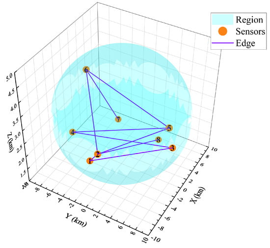
Figure 1. Multiple UAV nodes geometry and connectivity.

Table 1. Initial parameter settings.

UAV	Position (km)	Velocity (m/s)	Acceleration (m/s2)	DC	BC	CC
1	(−6.29,−1.54,2.05)	(200,0,0)	(0,0,0)	2	1.86	3.31
2	(−7.42,0.53,2.71)	(200,0,0)	(0,0,0)	4	3.86	4.60
3	(0.55,7.98,2.34)	(200,0,0)	(0,0,0)	2	1.29	2.50
4	(−3.72,−6.10,2.33)	(200,0,0)	(0,0,0)	2	1.57	3.00
5	(−0.69,7.80,3.28)	(200,0,0)	(0,0,0)	3	2.43	4.09
6	(−0.16,−5.65,−4.15)	(200,0,0)	(0,0,0)	3	2.71	3.67
7	(3.81,−2.81,1.97)	(200,0,0)	(0,0,0)	1	1.00	2.11
8	(3.67,4.25,1.81)	(200,0,0)	(0,0,0)	1	1.00	2.50
Target	(120,−15,4)	(−200,100,0)	(−1,0,0)	–	–	–

“–” represents no data in this cell.

The motion of the UAV networks followed the CA model. The velocities and accelerations of the UAVs were initialized as $(200,0,0)\mathrm{m}/\mathrm{s}$ and $(0,0,0)\mathrm{m}/{\mathrm{s}}^2$, respectively. The standard deviation $q_x,q_y,q_z$ of the process noise was set to $0.1\mathrm{m}/{\mathrm{s}}^2$ in the model.

The trajectory of the target evolved according to the CA models. The positions, velocities, and accelerations of the target were initialized as $(120,-15,4)\mathrm{km}$, $(-200,100,0)\mathrm{m}/\mathrm{s}$, and $(-1,0,0)\mathrm{m}/{\mathrm{s}}^2$, respectively. The standard deviation of position and process noise was set to be the same as the UAV networks.

The fusion period $T_F$ was defined as $0.5\mathrm{s}$ throughout the simulation duration of $200\mathrm{s}$. The filter initialization (i.e., initial state vector and covariance matrix) was calculated by the one-point initialization method in [6]. Numerical simulations are presented with 300 Monte Carlo runs.

4.2. Multiple UAV State Estimation

In this subsection, the consensus weighting matrix of the proposed DCE–ICI algorithm is compared with the Metropolis in [11]. The performance of the proposed DCE–ICI method is compared to the local estimation algorithm (Local) described in Section 2.2, the diffusion FCI (Diff–FCI), the diffusion ICI (Diff–ICI), and the distributed consensus estimation FCI (DCE–FCI). All methods used the same local estimation algorithm (i.e., Local) to ensure a fair performance comparison. The iterative NE of the consensus weighting matrix are shown in Figure 2. Figure 3 and Figure 4 show the RMSE of the target position and velocity estimation.

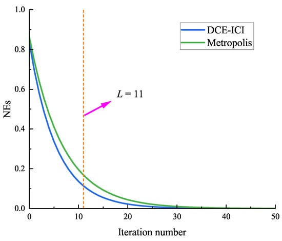
Figure 2. Iterative NE of different weights.

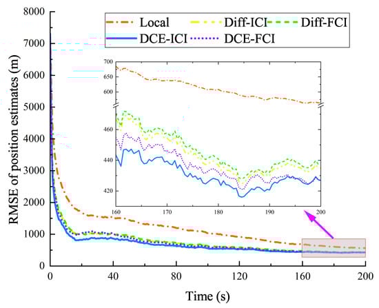
Figure 3. RMSE for position estimates (in the CA model).

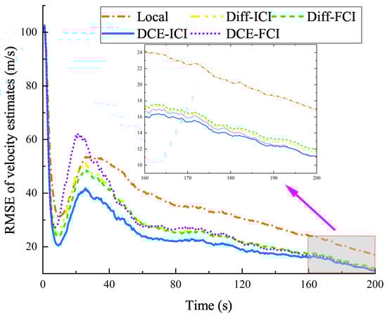
Figure 4. RMSE for velocity estimates (in the CA model).

As shown in Figure 2, the NE of weights in both methods (i.e., DCE–ICI and Metropolis) gradually converge to zero as the number of iterations increases. The trends of the above two curves are consistent with Remark 3. Under the same number of iterations, the value of the DCE–ICI method is smaller than that of Metropolis, which means that the proposed DCE–ICI method approaches the stable value (${\displaystyle \frac{1}{N}}\mathit{1}{\mathit{1}}^T$) faster and has better convergence performance. When the number of iterations reaches a finite number ($L=11$), the NE have not yet converged to zeros. Nevertheless, each row of the consensus weighting matrix ${\alpha }_i$ constitutes a valid set of coefficients satisfying the ICI fusion rule.

To demonstrate the tracking errors further, the RMSE of the position and velocity are shown in Figure 3 and Figure 4. The position and velocity RMSE of the proposed DCE–ICI method are smaller than those of all other methods. The performance of consensus-based methods (DCE) is generally better than that of diffusion (Diff) methods. Under the same distributed scheme (i.e., diffusion-based or consensus-based), the performance of the ICI fusion rule is superior to that of the CI fusion rule. In addition, Local and DCE–ICI methods performed best and worst, respectively. As listed in Table 2, the average RMSE of the position and velocity in the DCE–ICI method is approximately 684.19 m and 23.41 m/s. In the 0∼40 s interval, the RMSE of the velocity changed more sharply than that of the position. This is because, in the initial calculation of the filter, only the prior position information of the target can be obtained by the one-point initialization method, rather than the prior velocity information. Combining the results shown in Figure 3 and Figure 4 and Table 2, it is evident that the DCE–ICI method continuously provides accurate target state estimates, outperforming the other comparison distributed methods.

Table 2. Average RMSEs of different methods (in the CA model).

Term	Position (m)	Velocity (m/s)
Local	1183.60	34.67
Diff–ICI	764.47	27.02
Diff–FCI	773.68	26.65
DCE–ICI	684.19	23.41
DCE–FCI	746.86	28.13

4.3. Multiple UAV State Estimation with Different Target Maneuvering

In this subsection, we primarily performed the target state estimation in different maneuvering models. As shown in Table 3, the positions and velocities of the target were initialized as $(120,-15,4)\mathrm{km}$, and $(-200,50,0)\mathrm{m}/\mathrm{s}$, respectively. The accelerations of the target were initialized as $(-0.2,1,0)\mathrm{m}/{\mathrm{s}}^2$, $(-0.2,-1,0)\mathrm{m}/{\mathrm{s}}^2$, and $(-0.2,0,0)\mathrm{m}/{\mathrm{s}}^2$ in 0∼50 s, 50∼100 s, and 100∼200 s, respectively. Except for the maneuvering models, all remaining parameter settings are the same as the simulation experiment in Section 4.2. Figure 5 and Figure 6 illustrate the RMSE of the target position and velocity estimation in different maneuvering models. And Table 4 lists the average RMSEs of different methods.

Table 3. Target maneuvering parameters at different times.

Time (s)	Position (km)	Velocity (m/s)	Acceleration (m/s2)
0	(120,−15,4)	(−200,50,0)	(−0.2,1,0)
(0,50]	–	–	(−0.2,1,0)
(50,100]	–	–	(−0.2,−1,0)
(100,200]	–	–	(−0.2,0,0)

Position and velocity vary continuously over simulation duration.

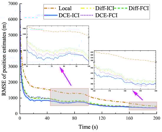
Figure 5. RMSE for position estimates (in different maneuvering models).

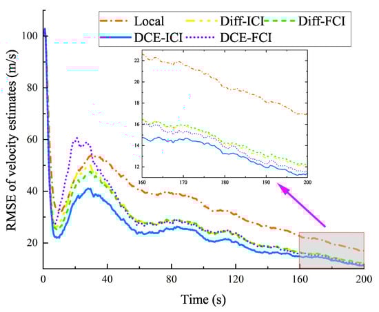
Figure 6. RMSE for velocity estimates (in different maneuvering models).

Table 4. Average RMSEs of different methods (in different maneuvering models).

Term	Position (m)	Velocity (m/s)
Local	1195.67	34.76
Diff–ICI	759.69	27.25
Diff–FCI	772.43	26.84
DCE–ICI	684.72	23.69
DCE–FCI	737.04	28.69

From Figure 5 and Figure 6, the position and velocity RMSE of the proposed DCE–ICI method are smaller than those of all other methods in different maneuvering models. The performance of consensus-based methods (DCE) is consistent with the simulation results in Section 4.2. The RMSE of the position and velocity changed sharply than that of the CA model, especially at 50 s and 100 s, when the acceleration of the target exhibits a sudden change. As listed in Table 4, the average RMSE of the position and velocity in the DCE–ICI method is approximately 684.72 m and 23.69 m/s. These results are very close to those obtained by the target that follows the CA model. Based on the results shown in Figure 5 and Figure 6 and Table 4, we can conclude that the DCE–ICI method can effectively achieve accurate target state estimates in different maneuvering models.

The simulations are conducted for a fixed communication topology. If the communication topology is a directed graph, some nodes may fail to receive information from their neighbors, making it difficult to achieve consensus. Therefore, as long as Assumption 1 holds, increasing or decreasing UAV nodes will not affect the output of the system. In practice, topology switching primarily impacts the consensus weight matrix in (65). Provided that each node can adaptively determine its own centrality, the proposed DCE–ICI method can effectively achieve consensus-based state estimation during topology transitions. Furthermore, a finite number of consensus iterations are performed at each fusion period (0.5 s), enabling each node to output a consensus estimate. A topology switch occurring at any given time does not affect subsequent consensus iteration estimates.

5. Conclusions

In this study, a DCE method with ICI fusion rule(DCE–ICI) is proposed in the framework of the local estimation and consensus iteration fusion for target tracking in multi-UAV systems. The proposed method can effectively and precisely achieve local estimation in bearing-only UAVs, even for invalid measurements. Based on centralities in a multi-UAV network, the proposed DCE–ICI method with novel consensus weighting matrix enables each UAV to obtain consensus results faster in a finite number of iterations. In addition to this, the fusion estimations have superior performance than the diffusion-based scheme and CI fusion. Simulation results indicate that the proposed method can effectively estimate target states. Compared with other existing distributed methods, the proposed method exhibits strong applicability in performing local estimation and can achieve significantly better estimation accuracy for maneuvering target tracking. These results highlight the effectiveness and superiority of the proposed method for distributed state estimation in bearing-only UAVs.

Subsequent work will focus on the following: (1) the study of consensus weighting matrix with faster convergence and investigation of deep reinforcement learning for calculating the optimal topology connection for UAV networks, and (2) application of the distributed consensus estimation method in a real experiment addressing the constraints of limited onboard computing cost, the stochastic nature of low-cost sensor noise, and potential environmental disturbances.

References

- Bassolillo, S.R.; D’Amato, E.; Notaro, I. A Consensus-Driven Distributed Moving Horizon Estimation Approach for Target Detection Within Unmanned Aerial Vehicle Formations in Rescue Operations. Drones 2025, 9, 127. [Google Scholar] [CrossRef]
- Sun, S.L. Distributed optimal linear fusion estimators. Inform. Fusion 2020, 63, 56–73. [Google Scholar] [CrossRef]
- Zhou, F.; Wang, Y.; Zheng, W.; Li, Z.; Wen, X. Fast Distributed Multiple-Model Nonlinearity Estimation for Tracking the Non-Cooperative Highly Maneuvering Target. Remote Sens. 2022, 14, 4239. [Google Scholar] [CrossRef]
- Liu, S.; Lin, Z.; Huang, W.; Yan, B. Current development and future prospects of multi-target assignment problem: A bibliometric analysis review. Def. Technol. 2025, 43, 44–59. [Google Scholar] [CrossRef]
- Guan, X.; Lu, Y.; Ruan, L. Joint Optimization Control Algorithm for Passive Multi-Sensors on Drones for Multi-Target Tracking. Drones 2024, 8, 627. [Google Scholar] [CrossRef]
- Yang, G.; Fu, W.; Zhu, S.; Wang, C.; Zhang, T. Online Spatial–Temporal Alignment Method in Bearing-Only Sensors for Maneuvering Target Tracking. IEEE Sens. J. 2025, 25, 7028–7042. [Google Scholar] [CrossRef]
- Zhang, Q.; Xie, Y.; Song, T.L. Distributed multi-target tracking with Y-shaped passive linear array sonars for effective ghost track elimination. Inform. Sci. 2018, 433–434, 163–187. [Google Scholar] [CrossRef]
- Cattivelli, F.S.; Sayed, A.H. Diffusion Strategies for Distributed Kalman Filtering and Smoothing. IEEE Trans. Autom. Control 2010, 55, 2069–2084. [Google Scholar] [CrossRef]
- Jia, B.; Sun, T.; Xin, M. Iterative Diffusion-Based Distributed Cubature Gaussian Mixture Filter for Multisensor Estimation. Sensors 2016, 16, 1741. [Google Scholar] [CrossRef]
- Sun, T.; Xin, M. Distributed Estimation With Iterative Inverse Covariance Intersection. IEEE Trans. Circuits Syst. II-Express Briefs 2023, 70, 1645–1649. [Google Scholar] [CrossRef]
- Xiao, L.; Boyd, S.; Lall, S. A scheme for robust distributed sensor fusion based on average consensus. In Proceedings of the 4th International Symposium on Information Processing in Sensor Networks, Los Angeles, CA, USA, 24–27 April 2005; pp. 63–70. [Google Scholar] [CrossRef]
- Li, W.; Wei, G.; Han, F.; Liu, Y. Weighted Average Consensus-Based Unscented Kalman Filtering. IEEE Trans. Cybern. 2016, 46, 558–567. [Google Scholar] [CrossRef] [PubMed]
- Zhang, Z.; Dong, X.; Yv, J.; Li, Q.; Ren, Z. Finite-time distributed state estimation for maneuvering target with switching directed topologies. J. Frankl. Inst. 2024, 361, 106695. [Google Scholar] [CrossRef]
- Julier, S.; Uhlmann, J. A non-divergent estimation algorithm in the presence of unknown correlations. In Proceedings of the 1997 American Control Conference, Albuquerque, NM, USA, 6 June 1997; Volume 4, pp. 2369–2373. [Google Scholar] [CrossRef]
- Wang, S.; Ren, W. On the Convergence Conditions of Distributed Dynamic State Estimation Using Sensor Networks: A Unified Framework. IEEE Trans. Control Syst. Technol. 2018, 26, 1300–1316. [Google Scholar] [CrossRef]
- Zhai, X.; Yang, Y.; Liu, Z. A Transformer-based Multi-Platform Sequential Estimation Fusion. Eng. Appl. Artif. Intel. 2025, 144, 110069. [Google Scholar] [CrossRef]
- Wang, Y.; Li, X.R. Distributed Estimation Fusion with Unavailable Cross-Correlation. IEEE Trans. Aerosp. Electron. Syst. 2012, 48, 259–278. [Google Scholar] [CrossRef]
- Chen, X.; Ji, J.; Wang, Y. Robust Cooperative Multi-Vehicle Tracking with Inaccurate Self-Localization Based on On-Board Sensors and Inter-Vehicle Communication. Sensors 2020, 20, 3212. [Google Scholar] [CrossRef]
- Niehsen, W. Information fusion based on fast covariance intersection filtering. In Proceedings of the 5th International Conference on Information Fusion, Annapolis, MD, USA, 8–11 July 2002; Volume 2, pp. 901–904. [Google Scholar] [CrossRef]
- Hays, C.W.; Henderson, T. Matrix decomposition approaches for mutual information approximation with applications to covariance intersection techniques. Inform. Fusion 2023, 95, 446–453. [Google Scholar] [CrossRef]
- Noack, B.; Sijs, J.; Reinhardt, M.; Hanebeck, U.D. Decentralized data fusion with inverse covariance intersection. Automatica 2017, 79, 35–41. [Google Scholar] [CrossRef]
- Ajgl, J.; Straka, O. Inverse Covariance Intersection Fusion of Multiple Estimates. In Proceedings of the IEEE 23rd International Conference on Information Fusion, Rustenburg, South Africa, 6–9 July 2020; pp. 1–8. [Google Scholar] [CrossRef]
- Sun, T.; Xin, M. Inverse-Covariance-Intersection-Based Distributed Estimation and Application in Wireless Sensor Network. IEEE Trans. Ind. Inform. 2023, 19, 10079–10090. [Google Scholar] [CrossRef]
- Chandra, K.P.B.; Gu, D.W.; Postlethwaite, I. Square Root Cubature Information Filter. IEEE Sens. J. 2013, 13, 750–758. [Google Scholar] [CrossRef]
- Chen, Z.; Fu, W.; Zhang, R.; Fang, Y.; Xiao, Z. Distributed Cubature Information Filtering Method for State Estimation in Bearing-Only Sensor Network. Entropy 2024, 26, 236. [Google Scholar] [CrossRef]
- Wang, S.; Li, Y.; Qi, G.; Sheng, A. Diffusion Nonlinear Estimation and Distributed UAV Path Optimization for Target Tracking with Intermittent Measurements and Unknown Cross-Correlations. Drones 2023, 7, 473. [Google Scholar] [CrossRef]
- Olfati-Saber, R. Distributed Kalman filtering for sensor networks. In Proceedings of the 46th IEEE Conference on Decision and Control, New Orleans, LA, USA, 12–14 December 2007; pp. 5492–5498. [Google Scholar] [CrossRef]
- Goh, K.I.; Oh, E.; Kahng, B.; Kim, D. Betweenness centrality correlation in social networks. Phys. Rev. E 2003, 67, 017101. [Google Scholar] [CrossRef]
- Liu, Z.; Ye, J.; Zou, Z. Closeness Centrality on Uncertain Graphs. ACM Trans. Web 2023, 17, 1–29. [Google Scholar] [CrossRef]
- Xiao, L.; Boyd, S. Fast linear iterations for distributed averaging. In Proceedings of the 42nd IEEE International Conference on Decision and Control, Maui, HI, USA, 9–12 December 2003; Volume 5, pp. 4997–5002. [Google Scholar] [CrossRef]
- Chen, Y.; Sheng, A.; Qi, G.; Li, Y. Diffusion self-triggered square-root cubature information filter for nonlinear non-Gaussian systems and its application to the optic-electric sensor network. Inform. Fusion 2020, 55, 260–268. [Google Scholar] [CrossRef]
Disclaimer/Publisher’s Note: The statements, opinions and data contained in all publications are solely those of the individual author(s) and contributor(s) and not of MDPI and/or the editor(s). MDPI and/or the editor(s) disclaim responsibility for any injury to people or property resulting from any ideas, methods, instructions or products referred to in the content. |
© 2026 by the authors. Licensee MDPI, Basel, Switzerland. This article is an open access article distributed under the terms and conditions of the Creative Commons Attribution (CC BY) license.