Abstract
The Fisheating Creek watershed located in Florida, United States of America (USA) is the focus of intense efforts to reduce nutrient transport into Lake Okeechobee which is located downstream. Public agencies and private land owners proposed constructing large nutrient removal basins in the watershed to reduce the overall nutrient load into Lake Okeechobee. This is challenging given the nature of the watershed with its low water availability and sensitivity to drought. This study evaluates the feasibility of implementing nutrient removal systems in such a watershed, including the overall risk and uncertainty of system performance. The study uses statistical evaluations of available water resources data and model simulations using Hydrologic Engineering Center Hydrologic Modeling System (HEC-HMS) to evaluate watershed flow conditions. Then, the study outlines alternatives for nutrient removal system implementation. The study revealed that considerable nutrient reduction is feasible but not optimal due to low overall water availability. The primary conclusion is that, while nutrient removal projects as large as 294 hectares can be constructed, the overall system operation will have to be very flexible to account for widely ranging inflows, including very low flows during drought situations.
Keywords:
nutrients; stormwater treatment areas; water availability; Fisheating Creek; Lake Okeechobee PACS:
J0101
1. Introduction
This article summarizes research regarding the feasibility of developing nutrient removal project alternatives on the Blue Head Ranch property within the Fisheating Creek watershed for the purposes of reducing nutrient loads into Lake Okeechobee, one of the largest freshwater lakes in the United States of America (USA). Some Supplementary materials are presented as S1 “Supplementary Material” for this paper. This research article is important, as the Fisheating Creek watershed is mostly commercially undeveloped and includes large swaths of undisturbed wetlands and extensive cattle ranch operations. Therefore, opportunities exist within the watershed to reduce nutrient use and nutrient loads which ultimately end up in Lake Okeechobee. However, the feasibility of nutrient removal projects is hindered by the frequent instances of low water availability within the watershed, especially during the dry season or extended droughts. The study uses statistical evaluations of available water resources data and model simulations using Hydrologic Engineering Center Hydrologic Modeling System (HEC-HMS) to evaluate watershed flow conditions. Then, the study outlines alternatives for nutrient removal system implementation. The study revealed that considerable nutrient reduction is feasible but not optimal due to low overall water availability. The primary conclusion is that while nutrient removal projects as large as 294 hectares can be constructed, the overall system operation will have to be very flexible to account for widely ranging inflows including very low flows during drought situations.
The Blue Head Ranch property consists of 127 km2 located in Highlands County, Florida, USA. The Blue Head Ranch is located within the Fisheating Creek watershed or basin on the northwestern side of Lake Okeechobee. Figure 1 shows the general location of the property in Florida, USA. Figure 2 shows the boundary of the Fisheating Creek watershed along with the property line for the Blue Head Ranch.
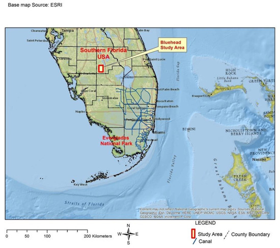
Figure 1.
Project location in Florida, United States of America (USA).
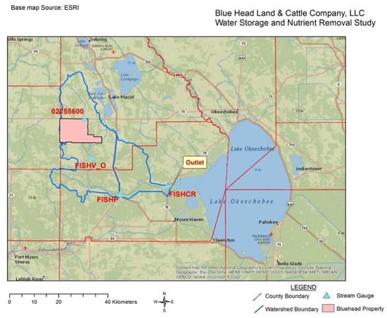
Figure 2.
Location of Fisheating Creek basin and the Bluehead Ranch property boundary.
The Fisheating Creek watershed is approximately 1124 km2 in size according to geographic information system (GIS) analyses completed for this study. Fisheating Creek flows with a gentle natural gradient of about 0.0095% from its source in Northern Highlands County south, and then east into Lake Okeechobee [1]. The upper portion of the basin contains significant amounts of agricultural land and cattle pastures, while the lower basin is dominated by large wetland areas like the Cowbone Marsh [2,3]. According to 1999 land-use surveys, the watershed is made of 70% agricultural production, pasture land, or rangeland, while about 27% consists of wetlands and forest [4].
While Fisheating Creek is designated an “Outstanding Florida Waters” basin, it is also classified as an impaired water source by the Florida Department of Environmental Protection [4] with high nutrient loads, low dissolved oxygen, and high iron. Since Fisheating Creek discharges into the Lake Okeechobee, it is subject to nutrient load reduction goals governed by the “Lake Okeechobee Operating Permit” (LOOP), which provides total phosphorus (TP) reduction goals for four regions around Lake Okeechobee [5]. Fisheating Creek is in the northern region of Lake Okeechobee which has an annual TP load target of 78.59 metric tons per year (MT/year) [5]. Overall, that means a target load reduction of about 212 MT/year TP for the northern region around Lake Okeechobee based upon 2012 TP estimates (e.g., a 73% reduction in TP loads discharging into the lake). Published TP load estimates entering Lake Okeechobee from Fisheating Creek watershed vary from about 41 MT/year [1] to 66.1 MT/year [5].
This study used both statistical analysis of real stream and rain data (see Figure 1 for stream gauge locations) and development of simple water budgets combined with model simulations to evaluate different nutrient reduction alternatives. Four alternatives were evaluated with several appearing to provide some moderate nutrient removal benefits for Lake Okeechobee.
2. Materials and Methods
The initial task undertaken for the study after developing a study overview was the inventory and analysis of available hydrologic data for the Fisheating Creek watershed. Both stream flow data and precipitation data were evaluated. Data from four stream gauges were reviewed to assess the available period of record (POR), data quality, and completeness. Table 1 shows the POR available for each gauge. Three out of the four gauges had data available through 2016. Gauge FishV_O only collected 11 years of flow data and was ultimately discontinued in 1967. However, the FishV_O gauge was very useful since the POR from 1955 to 1966 included some very dry periods. In addition to the stream gauge data, three different rain gauges were also studied and used in the model development. Key durations when both the stream gauge and rainfall data were available were flagged for use during model development.

Table 1.
Fisheating Creek stream gauge available data period of record (POR).
After collating the available data, the research attempted to estimate the overall water budget and nutrient mass budget within the Fisheating Creek watershed. Various datasets and existing literature were reviewed and analyzed to develop the overall water budget. Annual estimates were developed for the precipitation, evapotranspiration (ET), surface water runoff, consumptive use, infiltration, and overall change in basin storage. The water quality data available within the watershed were reviewed with a primary emphasis on nutrients including TP and total nitrogen (TN). The data were inventoried, evaluated, and then summarized in order to develop estimates of nutrient mass load at each stream gauge and for the entire watershed discharging into Lake Okeechobee.
Moreover, an HEC-HMS rainfall–runoff model [6,7] was developed for the watershed for the purpose of evaluating nutrient removal projects, including stormwater treatment areas (STAs). The model was calibrated and then validated using existing stream gauge data at the four gauges available for use, alongside the three rain gauges that cover the watershed. The model was simulated using the “continuous simulation” process as advocated by Shamsi and Koran [8]. This process is more challenging than event-based hydrologic rainfall–runoff models due to longer calibration and validation periods. For the model calibration period, the period from 3 March 1964 to 7 July 1966 was chosen based upon available precipitation data (three rain gauges in the watershed) and available stream gauge data at FishV_O and FishP. The calibration period was also drier than average with the mean annual precipitation at approximately 112 centimeters (cm) versus the long-term average of 132.44 cm. For the model validation period, the period from 1 January 2015 to 7 November 2016 was chosen due to data availability and for the fact that this period was considerably wetter than normal. During this period, the mean annual precipitation was about 152 cm versus the long-term average of 132.44 cm. This period also permitted the use of Nexrad-gauge-corrected precipitation data which involves using the Nexrad radar to estimate precipitation continuously across the watershed (https://www.sfwmd.gov/weather-radar/rainfall-historical/yearto-date). Each model simulation compared synthetic (simulated) hydrograph data to observed hydrograph data at available stream gauges.
For model development and calibration, both water budgets and goodness-of-fit parameters were calculated. The Nash–Sutcliffe efficiency coefficient (NSE) [9] compared the observed stream flows at each gauge versus the simulated flows. Then, the difference between the two values was calculated. The goal of model calibration was to minimize the difference such that the model-predicted flow rate was about the same as the observed flow rate during the period of record modeled, while ensuring the overall water mass budgets were similar as well. During calibration, the residual difference between the predicted model flow and actual observed flow was continually reduced in the model by revising various input parameters including the curve number (CN), initial abstraction, storage volume, ET, and baseflow.
The NSE is a normalized statistic that determines the relative magnitude of the residual variance compared to the measured data variance and indicates how well the plot of the observed data versus the simulated data fits the 1:1 line [10]. Although this statistic is mostly used to compare simulated discharges versus modeled discharges in hydrologic models, it can also be used to compare simulated stages versus observed stages. The NSE equation can be seen below in Equation (1).
where Oi is the observed data on the ith day, Si is the simulated data on the ith day, Obar is the observed mean value, and n is the number of observations
The ranges for NSE can vary between −∞ and 1, where NSE = 1 corresponds to a perfect match between simulated data and observed data, NSE = 0 shows that the model predictions are as accurate as the mean of the observed data, and −∞ < NSE < 0 occurs when the observed mean is a better predictor than the model, which indicates unacceptable performance [10].
Since this model is a preliminary version to be used for planning and preliminary design, the research team established the following realistic calibration goals:
- Simulated flow budgets matched at each gauge within 15% of observed values;
- NSE coefficient goodness-of-fit statistics for all model stream gauges greater than or equal to 0.3.
These goals are consistent with other recent model calibration guidance. For example, one source of model calibration criteria is the Wastewater Planning Users Group Code of Practice for the Hydraulic Modeling of Sewer Systems [11]. This guidance document suggests matching water mass budgets at ±10% for dry periods and −10% to +20% for wet periods. Other researchers suggest the appropriate range of NSE coefficients for planning purposes and preliminary design to be at least 0.30 to 0.39 [8]. Values greater than 0.5 are considered “excellent” for calibration purposes, permitting even final design use of the model. The St. Johns River Water Supply Impact Study [12] completed by the Saint Johns River Water Management District (SJRWMD) used the NSE to “rank” the calibration performance for their hydraulic model. Following their methodology, the NSE values can be divided into intervals which explain the model performance rating. The intervals are as follows: 0.75 < NSE < 1 is a “very good” performance rating, 0.65 < NSE < 0.75 is a “good” performance rating, and 0.50 < NSE < 0.65 is a “satisfactory” performance rating. NSE values that are negative are unacceptable.
Finally, once the actual field data were analyzed and the hydrologic model was calibrated, they were used to develop preliminary designs for stormwater treatment areas designed to remove TP and TN from Fisheating Creek for the purpose of reducing the total nutrient load into Lake Okeechobee. Ultimately, four alternatives were assessed and compared.
3. Results
3.1. Inventory and Analysis of Real Field Data
The stream flow data from the four stream gauges used in the watershed were analyzed using a frequency analysis to determine the portion of the POR where mean daily flow exhibited the following characteristics:
- Less than 0.708 cubic meters per second (m3∙s−1);
- Less than 2.83 m3∙s−1;
- Greater than 28.32 m3∙s−1.
Table 2 shows the results of the frequency analysis.
Table 2.
Frequency analysis of four stream gauges in Fisheating Creek.
It is clear from Table 2 data that any diversions of flow from Fisheating Creek must be managed carefully due to the generally low-to-moderate flow available during most periods. The potential adverse effects of any project in dry season conditions is of particular importance as a design constraint. For the Blue Head Ranch, gauges 0255600 and FishV_O bracket the property and represent available water for storage and/or treatment. In reviewing the frequency of high flows at gauge 0255600, which is just upstream of the northern boundary of Blue Head Ranch, the data indicate that, in any given year, one could expect flows of greater than 2.83 m3∙s−1 to occur for only about 56 days. Of course, in dry years, it would likely be less than 56 days. Similarly, flow data at FishV_O indicate flows greater than 2.83 m3∙s−1 occur only about 91 days per year. Since the Blue Head Ranch southern boundary is about mid-way between these two gauges, it is estimated that flows greater than 2.83 m3∙s−1 occur about 74 days per year at that location or an average of the durations calculated at each gauge.
In addition to the frequency analysis, the overall mean and median flows were calculated at each stream gauge. Table 3 depicts the results at each gauge location.
Table 3.
Flow statistics for each stream gauge.
Table 3 clearly demonstrates that the stream flow datasets are highly non-normal and that median values probably represent the most reliable flow statistic for central-tendency comparison purposes. Also, it is evident from Table 3 that the overall flows within Fisheating Creek are low to moderate. The location of the Bluehead Ranch property is between stream gauge 0255600 and gauge FishV_O, meaning that a median flow of 0.48 m3∙s−1 or less would be expected under normal conditions. Furthermore, in reviewing the location of various sub-basins within the Fisheating Creek, it is clear that any engineered nutrient removal projects located on the Bluehead Ranch property would be constrained by the availability of water from certain sub-basins or portions of the main stem Fisheating Creek. Figure 3 depicts the location of the key sub-basins important to the Bluehead Ranch property. The figure shows that the Bluehead Ranch can only really exert a positive effect on six sub-basins within the Fisheating Creek watershed, including portions of the main creek stem.
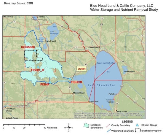
Figure 3.
Location of various watershed sub-basins near the Bluehead Ranch property boundary.
3.2. Water and Nutrient Mass Budget Development
Another important consideration in the Fisheating Creek watershed is the overall water budget in the area. The water budget delineates where precipitation that falls on the watershed ends up. Precipitation may be infiltrated or percolated into the surficial aquifer system (SAS), evaporated or transpired into the atmosphere, used consumptively for water supply or irrigation, and/or runoff into area streams and rivers. The overall water budget provides important information when considering alternative water storage projects in the watershed and constrains simulation models built to assess the potential projects. The Southwest Florida Water Management District (SWFWMD) summarized precipitation for all counties in its service area (https://www.swfwmd.state.fl.us/data/hydrologic/rainfall_data_summaries/), including Highlands County which covers a large portion of the Fisheating Creek watershed. For Highlands County, the mean annual precipitation is about 132.44 cm. This is the precipitation (P) assumed for the general watershed water budget input for this study. Evaporation from open water and transpiration by vegetation account for the largest flow output in the overall water budget. The combined term, called evapotranspiration (ET), can be as high as 182.88 cm per year as a maximum potential. However, usually, ET does not attain its maximum due to variations in solar radiation, wind, shade, groundwater depth, and type of vegetation. The research team reviewed and summarized ET data in the study area and from published reports from nearby watersheds. Abtew et al. provided a general estimate of actual ET in south Florida [13]. Mao et al. provided an estimate of actual ET in the Upper St. Johns River watershed, which is similar in many ways to the Fisheating Creek watershed [14]. The Loinaz data were determined from model calibration in the Fisheating Creek for late 1990s data [2]. The Metcalf and Eddy/AECOM data probably represent the maximum ET possible in the Fisheating Creek watershed [1]. For this study, and based upon the published ET values, it was assumed that the actual ET within Fisheating Creek ranges from 73.66 cm per year 134.62 per year, with 73.66 cm per year assumed for the initial water budget. During HEC-HMS model calibration, the ET value was varied in order to determine the best match to observed flows at each of the four stream gauges.
Estimates for annual average runoff (RO) for the watershed are also available within the watershed. Rumenik estimated about 25.4 to 30.48 cm per year of annual runoff in Fisheating Creek watershed [15]. Additional runoff estimates completed for this study using the four stream gauges mentioned previously revealed estimates ranging from 22.86 to 30.48 cm per year. For the sake of the water budget analysis, it was assumed that runoff is 27.94 cm per year on average. The remaining terms in the overall water budget for the watershed include infiltration (INF), consumptive water use (WD), and change in basin storage (DS). These values are not known a priori and must be estimated using the HEC-HMS model. Change in basin storage can be assumed to be zero over a long-term average (e.g., at steady-state conditions), but will vary year to year in the short term. Therefore, the following basic water budget can be developed as Equation (2):
P − ET − RO − INF − WD = DS,
or
132.44 cm (P) − 73.66 cm (ET) − 27.94 cm (RO) = INF + WD + DS = 30.84 cm.
or
132.44 cm (P) − 73.66 cm (ET) − 27.94 cm (RO) = INF + WD + DS = 30.84 cm.
Thus, it appears that average annual combined infiltration, consumptive use, and change in watershed storage is about 30.84 cm across the watershed. This equates to a daily flow equivalent of 10.97 m3∙s−1. The Loinaz study looked at opportunities for environmental restoration within the Fisheating Creek watershed through model simulations and determined that turning off drainage canals in order to raise the natural water table would provide about 3.12 m3∙s−1 of additional average daily flow back to Fisheating Creek [2]. Another way to interpret this model result is to assume that the 3.12 m3∙s−1 is currently being withdrawn for consumptive use purposes in the basin.
Taking that value into account (which can be normalized across the basin as about 8.76 cm per year), the water budget assessment points to 22.08 cm per year of infiltration and change in storage on average, or about 17% of the mean annual precipitation. Therefore, in drier years, there may be less infiltration generating less flow in the Fisheating Creek. This would tend to lead to a limitation of available “base flow” from the surficial aquifer back to Fisheasting Creek during drier years, and the observed stream gauge hydrographs bear this out showing very low flow or even zero flow for months at a time within Fisheating Creek during the dry season from October to May each year, or longer during drought years. This is an especially important finding from this study and means that, for any reservoir or nutrient removal project, water withdrawals will be limited by the availability of suitable higher flows in the creek.
Water quality data collected within Fisheating Creek, primarily focused upon nutrients, were also compiled and assessed for this study. Florida Department of Environmental Protection (FDEP) estimated a mean TP concentration of 0.162 mg/L from 351 historic water quality samples in the watershed [4]. FDEP also estimated a mean total nitrogen (TN) concentration of 1.62 mg/L from 331 historic samples [4]. A study by Graves showed the mean concentration of TP in the C-44 basin (east of Lake Okeechobee) to be 0.137 to 0.210 mg/L using different environmental databases [16]. Graves et al. estimated the median values of TP and TN for various land use in the C-44 basin [17]. Median values of TP in stormwater runoff from citrus lands (also important in the Fisheating Creek watershed) were estimated at 0.160 mg/L, while a value of 1.23 mg/L was determined for TN [17].
As part of the Lake Okeechobee Watershed Project and the Lake Okeechobee Watershed Assessment (LOWA) study [1], SFWMD collected water quality data since about 2004 at stations all around the Fisheating Creek watershed. Figure 4 shows a summary of the data with the sampling station locations shown, as well as the median total phosphorus (TP) concentration calculated at each water quality station. The figure also depicts the estimated TP annual load calculated at each stream gauge, along with the percentage of the total annual TP load entering Lake Okeechobee.
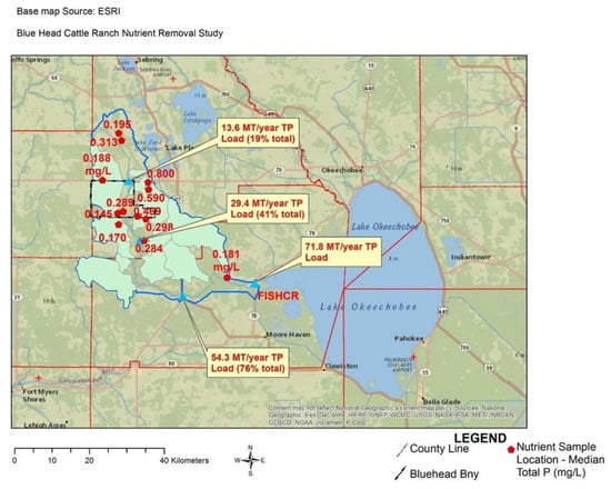
Figure 4.
Location of water quality stations in the study area.
TP median concentrations range from 0.145 mg/L to 0.80 mg/L. Two stations along the main stem of Fisheating Creek reveal a long-term median concentration of about 0.287 mg/L TP. Combining these data with the flow data discussed previously, the research team developed the annual TP nutrient mass load estimates shown in Figure 4. These annual TP load estimates are higher than previous estimates and probably represent a maximum nutrient load. Published TP load estimates entering Lake Okeechobee from Fisheating Creek watershed vary from about 41 MT/year [1] to 66.1 MT/year [5]. In carefully reviewing the estimate contributed by Metcalf and Eddy/AECOM, the research team noted that the mean flow used was considerably less than that determined for this study using a longer POR. If the Metcalf and Eddy/AECOM TP estimate is adjusted to account for higher average annual flows calculated from the current research, the TP load would be approximately 54 MT/year instead of 41 MT/year. Therefore, the current total TP annual load estimate (e.g., 71.8 MT/year) derived in this study is 8.6% greater than the Goforth estimate and about 33% greater than the adjusted Metcalf and Eddy/AECOM estimate. In light of these differences, the current estimate probably represents a maximum TP load, while the average load probably varies in a range from 54 MT/year to 71.8 MT/year. Total annual nitrogen mass load estimates from Fisheating Creek basin to Lake Okeechobee probably range from about 432 to 718 MT/year, assuming a TN/TP ratio ranging from 8 to 10, which would be consistent with data from past studies [4].
3.3. HEC-HMS Model Development, Calibration, and Validation
Several weeks were expended developing the model and then working through model calibration and validation. Table 4 displays the final calibration and validation goodness-of-fit statistics.
Table 4.
Model goodness-of-fit statistics for each stream gauge. NSE—Nash–Sutcliffe efficiency.
As demonstrated in the table, the model meets all of the calibration goals and, therefore, can be used for planning and preliminary design purposes. Figure 5 and Figure 6 show model hydrographs from the calibration and validation periods comparing simulated flows in blue and observed (actual) flows in black. Note that the graphs were taken from a published report for the client, and the units are in cubic feet per second (ft3∙s−1) as per the client’s request.
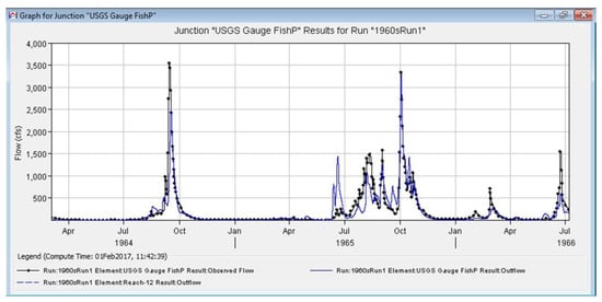
Figure 5.
Comparison of model simulation results and observed results at gauge FishP for the calibration period.
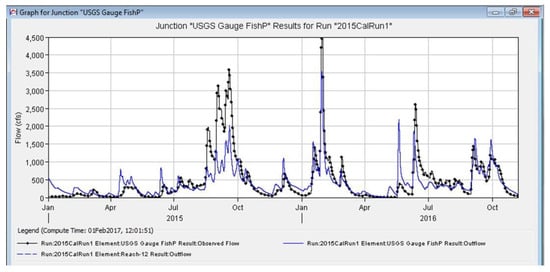
Figure 6.
Comparison of model simulation results and observed results at gauge FishP for the validation period.
3.4. Development and Evaluation of Nutrient Removal Alternatives
The research team developed and evaluated four nutrient removal alternatives as part of the study. The alternatives ranged in size from about 51 hectares to 294 hectares. Each was designed to include an initial equalization cell, followed by parallel stormwater treatment trains, using a combination of submerged and/or floating plants. In addition, the alternatives were stipulated to include variable speed discharge pump stations in order to cover inflow rates ranging from 0.02 to 1.5 m3∙s−1. Also, water outlet control structures were envisioned to have the ability to pond a minimum depth of water in each treatment cell to ensure efficacy of the wetland plant-based treatment design. Each alternative was assessed for its overall nutrient removal efficiency based upon the work of Wetland Solutions Inc. [18] and observed STA performance characteristics documented by Hazen and Sawyer [19]. Table 5 lists the expected range of nutrient removal performance of each alternative along with alternative size, estimated total first cost, and annual operating cost.
Table 5.
Expected nutrient removal performance of four alternatives. TP—total phosphorus.
The alternatives provide a range of performance characteristics, as well as first costs and operating costs. However, due to the unique nature of water availability within the basin, any of the alternatives will need to include maximum flexibility to ensure they are sustainable.
4. Discussion
Overall, the four alternatives that were evaluated in this report can remove 0.53 to 4.16 MT/year of TP and an additional 10.56 to 17.83 MT/year of TN. The overall capital cost and operation and maintenance (O&M) costs to build and operate the facilities is moderate, but operational costs are not optimal due to the low water flow conditions which predominate this part of the Fisheating Creek watershed. However, the estimated unit removal costs are in the expected range of actual unit removal costs published for active STA projects [19].
The overall potential benefit of the proposed STA project is substantial. If Alternative 3 was selected for implementation, as much as 6.3% of the total TP load generated in the Fisheating Creek watershed would be removed from Lake Okeechobee every year. Furthermore, the 4.16 MT/year could represent up to 8.6% of the LOOP-required TP load reduction targeted for the Fisheating Creek watershed. The unit removal cost is just one way to assess the value of the nutrient removal projects. RTI, working for the Everglades Foundation, estimated the value of nutrient removal based upon different possible treatment options [20]. They also calculated the true TP removal cost for the Everglades Construction Project (ECP), a massive STA system south of Lake Okeechobee, at $533,981 per metric ton. Therefore, for Alternative 3, the overall value of the TP removed could be as high as $2,221,361 per year using similar reasoning. In this light, the Alternative 3 project would pay for itself in about four years. Similarly, Alternative 4 TP removal could be valued at $1,644,662 per year and could recoup its initial costs in about three years.
A key constraint will likely be the availability of water within the watershed. The watershed already exhibits very low or no flows during the dry season and during drought conditions. If groundwater withdrawals from the watershed increase in the future, low- or no-flow conditions are expected to worsen, thus rendering STA projects possibly infeasible. Future planning of any proposed STA facilities should closely examine system operation under low-flow conditions.
Supplementary Materials
The following are available online at www.mdpi.com/xxx/s1: PowerPoint slides.
Author Contributions
C.B. led the research efforts for this article as part of his research program. The conceptualization of the work was performed by C.B. The model simulations were prepared and run by C.B. The formal analysis was completed by C.B. with some minor support from undergraduate student Jose Kolb-Lugo. This article was written by C.B. C.B. provided project administration and final article editing. All authors have read and agreed to the published version of the manuscript.
Funding
This research was funded by Foley & Lardner and the Blue Head Land & Cattle Company, LLC, grant index number 230395.
Acknowledgments
The author would like to acknowledge the South Florida Water Management District for sharing water quality data collected within the watershed.
Conflicts of Interest
The author declares no conflict of interest. The funders had no role in the design of the study; in the collection, analyses, or interpretation of data; in the writing of the manuscript, or in the decision to publish the results.
References
- Metcalf & Eddy/AECOM. Fisheating Creek Sub-Watershed Feasibility Study Phase I (Contract No. 4600000912WO01); Report Prepared for the South Florida Water Management District, South Florida Water Management District: West Palm Beach, FL, USA, 2009; 183p.
- Loinaz, M. Integrated Surface Water and Groundwater Model to Valuate Wetland Restoration and Water Storage Increase in the Fisheating Creek Basin. Master’s Thesis, University of Florida, Gainesville, FL, USA, May 2005. [Google Scholar]
- Nature Conservancy. Fisheating Creek Watershed Special Project Update; Nature Conservancy: Maitland, FL, USA, 2010; 19p. [Google Scholar]
- FDEP. Water Quality Assessment Report, Kissimmee River and Fisheating Creek; Florida Department of Environmental Protection: Tallahassee, FL, USA, 2006; 472p.
- Goforth, G. Presentation on the Lake Okeechobee Operating Permit Given to the South Florida Water Management. 2014. Available online: http://www.garygoforth.net/Draft%20-%20LOW%20Presentation%20-%208%207%202013%20-%20rev.pdf (accessed on 15 October 2018).
- U.S. Army Corps of Engineers. Hydrologic Modeling System HEC-HMS, Rep. No. CPD-74B; at 145; Hydrologic Engineering Center, Engineer Research and Development Center: Davis, CA, USA, 2000. [Google Scholar]
- Scharffenberg, W.A.; Fleming, M.J. Hydrologic Modeling System HEC-HMS User’s Manual; Army Corps of Engineers, HEC: Davis, CA, USA, 2010.
- Shamsi, U.M.; Koran, J. Continuous calibration. J. Water Manag. Model. 2017, 1–10. [Google Scholar] [CrossRef]
- Nash, J.E.; Sutcliffe, J.V. River Flow forecasting through conceptual models, 1, A discussion of principles. J. Hydrol. 1970, 10, 282–290. [Google Scholar] [CrossRef]
- Wang, W.C.; Chau, K.W.; Cheng, C.T.; Qiu, L. A comparison of performance of several artificial intelligence methods for forecasting monthly discharge time series. J. Hydrol. 2009, 374, 294–306. [Google Scholar] [CrossRef]
- WaPUG. Code of Practice for Hydraulic Modeling of Sewer Systems Version 3.001; Amended December 2002; Wastewater Planning Users Group: London, UK, 2002; Available online: http://www.ciwem.org/wpcontent/uploads/2016/05/Code-of-Practice-for-the-Hydraulic-Modelling-of-Sewer-Systems.pdf (accessed on 15 October 2018).
- St. Johns River Water Management District. St. Johns River Water Supply Impact Study; (Publication No. SJ2012-1); St. Johns River Water Management District: Palatka, FL, USA, 2012. [Google Scholar]
- Abtew, W.; Obeysekera, J.; Iricanin, N. Pan Evaporation and Potential Evapotranspiration Trends in South Florida; SFWMD Technical Paper # 107; South Florida Water Management District: West Palm Beach, FL, USA, 2010; 24p.
- Mao, L.M.; Bergman, M.J.; Tai, C. Evapotranspiration Measurement and Estimation of Three Wetland Environments in the Upper St. Johns River Basin, Florida. J. Am. Water Res. Assoc. 2002, 5, 1271–1285. [Google Scholar] [CrossRef]
- Rumenik, R.P. Runoff to Streams in Florida [Map]; Florida Geological Survey: Tallahassee, FL, USA, 1988.
- Graves, G. Estimation of contribution of total phosphorus from selected landuses to observed concentrations in tributaries to a coastal lagoon: Indian River Lagoon, Florida USA. In Proceedings of the National Stormwater Association 2002 Conference, Naples, FL, USA, August 2002. 15p. [Google Scholar]
- Graves, G.A.; Wan, Y.; Fike, D.L. Water Quality Characteristics of Storm Water from Major Land Uses in South. J. Am. Water Res. Assoc. 2004, 40, 1405–1419. [Google Scholar] [CrossRef]
- Wetland Solutions Inc. Development of Design Criteria for Stormwater Treatment Areas (STAs) in the Northern Lake Okeechobee Watershed; Report Prepared by the South Florida Water Management District, South Florida Water Management District: West Palm Beach, FL, USA, 2009; 144p.
- Hazen and Sawyer. Compilation of Benefits and Costs of STA and Reservoir Projects in the South Florida; Water Management District, Report Prepared for the World Wildlife Fund: Denver, CO, USA, 2011; 66p. [Google Scholar]
- RTI International. Enterprise Assessment for the Reduction of Nutrient Pollution in South Florida Waters; Final Report; Prepared for the Everglades Foundation: Miami, FL, USA, 2012; 107p. [Google Scholar]
Publisher’s Note: MDPI stays neutral with regard to jurisdictional claims in published maps and institutional affiliations. |
© 2018 by the author. Licensee MDPI, Basel, Switzerland. This article is an open access article distributed under the terms and conditions of the Creative Commons Attribution (CC BY) license (https://creativecommons.org/licenses/by/4.0/).