Hausdorff Outer Measures and the Representation of Coherent Upper Conditional Previsions by the Countably Additive Möbius Transform

Abstract

This paper explores coherent upper conditional previsions, a class of nonlinear functionals that generalize expectations while preserving consistency properties. The study focuses on their integral representation using the countably additive Möbius transform, which is possible if coherent upper previsions are defined with respect to a monotone set function of bounded variation. In this work, we prove that an integral representation with respect to a countably additive measure is also possible, on the Borel $\sigma$-algebra, even when the coherent upper prevision is defined by the Choquet integral with respect to a Hausdorff measure, which is not of bounded variation. It occurs since Hausdorff outer measures are metric measures, and therefore every Borel set is measurable with respect to them. Furthermore, when the conditioning event has a Hausdorff measure in its own Hausdorff dimension equal to zero or infinity, coherent conditional probability is defined via the countably additive Möbius transform of a monotone set function of bounded variation. The paper demonstrates the continuity of coherent conditional previsions induced by Hausdorff measures.

1. Introduction

In classical decision theory and probabilistic modeling, preference orderings and equivalence classes over uncertain outcomes are often represented using linear expectation operators associated with countably additive probability measures. However, it has long been recognized that such linear representations are inadequate for capturing many forms of ambiguity, imprecision, and risk attitudes observed in practical decision-making scenarios [1,2,3].

To address these limitations, a variety of nonlinear functionals have been introduced, including coherent upper and lower conditional previsions, which generalize the notion of expectation [4,5] by relaxing linearity while preserving certain consistency properties. These functionals provide a richer and more flexible framework for representing preferences that are not necessarily expressible through a single probability measure. Monotone set functions [6,7,8] and nonlinear integral [9,10] have been investigated in the literature. This paper focuses on a specific class of such functionals—coherent upper conditional previsions—and investigates their integral representations in terms of the countably additive Möbius transform. This integral representation is possible when uncertainty is represented by a monotone set function of bounded variation, that is, when coherent upper conditional previsions are defined with respect to a coherent upper probability of bounded variation. A first issue we address in this work is whether it is possible to represent the Choquet integral [11], with respect to a monotone set function $\mu$—not necessarily of bounded variation—using a countably additive measure, atleast on suitable domains. We investigate whether it is possible to find conditions under which the Choquet integral can be equivalently expressed through a countably additive measure, even when the underlying capacity lacks bounded variation. The answer to this question is affirmative, and a concrete example is provided by the framework of coherent conditional previsions constructed via Hausdorff outer measures.

In particular, the model of coherent conditional prevision based on Hausdorff outer measures illustrates how such a representation can be achieved, despite the absence of bounded variation in $\mu$ (Theorem 10).

This example demonstrates that under certain conditions, it is indeed possible to reconcile non-additive integration with classical measure theory. A central contribution of this work is the examination of the role played by Hausdorff outer measures in this context. We demonstrate that these outer measures provide a natural and powerful tool for defining coherent upper conditional previsions, which satisfy a Continuity Principle, particularly in settings where regularity conditions on the underlying space are relaxed. In fact, Hausdorff outer measures ${\mathcal{H}}^s$ for $0<s<1$ are proven to not be of bounded variation. Through this investigation, we aim to deepen the understanding of the interplay between non-additive measure theory and nonlinear expectation functionals, and to provide new mathematical foundations for applications in robust statistics, imprecise probabilities, and decision theory. A second result of this work is the introduction, on the Borel sigma-field, of a countably additive model of conditional prediction. This model is constructed by considering the countably additive Möbius transform of a monotone set function of bounded variation in cases where the conditioning event has a Hausdorff measure equal to 0 or ∞ in its Hausdorff dimension.

The continuity property of the conditional prediction depends on whether the monotone function is continuous from below. Given a monotone set function $\mu$ of bounded variation, defined on an algebra of events, it is possible to construct a sigma-additive probability on a suitable $\sigma$-algebra such that the Choquet integral defined with respect to $\mu$ is equal to an integral defined with respect to a $\sigma$-additive probability. This representation of the Choquet integral can be given by constructing a $\sigma$-additive representation of the monotone function $\mu$ using the $\sigma$-additive Möbius transform. Moreover, since the Choquet integrals are preserved under the Möbius transform, the two integral representations coincide. The construction of the $\sigma$-additive Möbius transform (see Lemma 6.1 and Theorem 6.2 of [12]) is obtained by considering the Möbius transform defined on an opportune $\sigma$-field where all finitely additive functions are continuous from above to the empty set and so countably additive. It is the same procedure used in [13] based on Theorem 2.3 of [14]. The construction of the Möbius transform is based on the Stone extension of a space $(\Omega ,\mathcal{A})$, where $\mathcal{A}$ is a field, to the measurable space $({\mathcal{H}}_p,{\mathcal{D}}^{\prime }\left(\mathcal{A}\right))$ of all supermodular 0–1 valued set functions. In this measurable space, each finite additive function is countably additive since it is continuous from above to the empty set.

A different construction of the Möbius transform of a monotone set function is proposed by using a composition norm so that any monotone set function can be expressed as a combination of particular coherent lower probabilities as the canonical representation of a game by unanimity games investigated in [15,16].

In this paper, the $\sigma$-additive Möbius transform is considered to propose a model of coherent countably additive conditional probability on the Borel $\sigma$-field (Theorem 4); we also prove that coherent lower conditional previsions defined with respect to the Möbius transform of a coherent lower probability $\nu$ are continuous if $\nu$ is continuous from below (Theorem 8) so that the monotone convergence theorem for monotone set functions (Theorem 5) holds.

The integral representation with respect to the $\sigma$-additive Möbius transform of belief functions has been investigated in [17,18]. In this paper, the general case of the integral representation with respect to a $\sigma$-additive probability of the Choquet integral is considered.

2. Preliminaries

Given a non-empty set $\Omega$ and denoted by $\wp (\Omega )$, the family of all subsets of $\Omega$, a monotone set function, also called capacity, $\mu :\wp (\Omega )\to {\overline{\Re }}_{+}={\Re }_{+}\cup \left\{+\infty \right\}$, is such that $\mu$(⊘) = 0, and if A, B∈$\wp (\Omega )$ with A⊂B, then $\mu$(A) ≤$\mu$ (B).

Let $\mathcal{F}$ be a field of subsets of $\Omega$, i.e., a collection of sets closed under finite unions, finite intersections, and relative complements. A monotone set function $\mu$ is supermodular or 2-monotone if

$$\mu (A\cup B)+\mu (A\cap B)\ge \mu \left(A\right)+\mu \left(B\right)$$

A set function $\mu$ is said to be k-monotone if for every collection of sets $A_1,A_2,\dots ,A_k\subseteq \Omega$, the following inequality holds:

$$\mu \left(\bigcup _{i=1}^k{A}_i\right)\ge \sum _{\varnothing \ne J\subseteq \{1,\dots ,k\}}{(-1)}^{\left|J\right|+1}\mu \left(\bigcap _{j\in J}{A}_j\right).$$

A set function $\mu$ is totally monotone if it is monotone and k-monotone for $k\ge 2$. A set function $\mu$ is a belief function if it is totally monotone and $\mu (\Omega )=1$.

A set function $\mu :\mathcal{F}\to [0,\infty ]$ is called a measure on the field $\mathcal{F}$ if it satisfies the following properties:

1. $\mu (\varnothing )=0$.

2. Countable additivity:

For any disjoint sets $A_1,A_2,\dots \in \mathcal{F}$ and ${\bigcup }_{n=1}^{\infty }{A}_n\in \mathcal{F}$, we have

$$\mu \left(\bigcup _{n=1}^{\infty }{A}_n\right)=\sum _{n=1}^{\infty }\mu \left(A_n\right).$$

$\mu$ is a probability measure on $\mathcal{F}$ if $\mu$ is a measure such that $\mu (\Omega )=1.$

Let $\mu$ be a probability measure. Then, the following properties hold (Theorem 2.1 [14]):

1. Continuity from below: If $A_1\subset A_2\subset \dots$ is an increasing sequence of events such that ${\bigcup }_{n=1}^{\infty }{A}_n\in \mathcal{F}$, then

$$\mu \left(\bigcup _{n=1}^{\infty }{A}_n\right)=\underset{n\to \infty }{lim}\mu \left(A_n\right).$$

2. Continuity from above: If $B_1\supset B_2\supset \dots$ is a decreasing sequence of events such that ${\bigcap }_{n=1}^{\infty }{B}_n\in \mathcal{F}$, then

$$\mu \left(\bigcap _{n=1}^{\infty }{B}_n\right)=\underset{n\to \infty }{lim}\mu \left(B_n\right).$$

3. Countable subadditivity: For any countable sequence of events $A_1,A_2,A_3,\dots \in \mathcal{F}$ pairwise disjoint

$$\mu \left(\bigcup _{n=1}^{\infty }{A}_n\right)\le \sum _{n=1}^{\infty }\mu \left(A_n\right).$$

In the presence of finite additivity, a special case of continuity from above implies countable additivity.

Proposition 1.

If μ is a finitely additive measure that is continuous, from above to ∅ on the field $\mathcal{F}$, then μ is countably additive. That is, if $B_1\supset B_2\supset \dots$ is a decreasing sequence of events such that ${\bigcap }_{n=1}^{\infty }{B}_n=\varnothing$ and $li{m}_{n\to \infty }\mu \left(B_n\right)=0$, then μ is countably additive.

One important condition that characterizes the countable additivity of finite measures is continuity from above to the empty set. The vanishing of the measure on decreasing sequences of sets tending to the empty set guarantees that $\mu$ behaves well under countable unions and disjoint decompositions, which are essential aspects of countable additivity. A countably additive probability measure can be defined on the $\sigma$-field generated by the field of all cylinders in the space of infinite sequences. This is achieved using a procedure based on Theorem 2.3 of [14], which proves that every finitely additive probability measure on the field of all cylinders in this space is, indeed, countably additive.

The key reason is that any sequence of non-empty cylinders converges to a non-empty set. Consequently, any finite probability measure is continuous from above to the empty set. According to Proposition 1, this implies countable additivity.

However, the same procedure cannot be applied to define a conditional probability in the continuous case. This is due to the fact that the $\sigma$-field generated by the field of all cylinders in the space of infinite sequences is closely related to the Borel $\sigma$-field on $[0,1]$, though significant differences exist.

In particular, the field of cylinders is strictly smaller than the field of finite disjoint unions of intervals in $(0,1]$, and in this case, Theorem 2.3 does not always apply. Specifically, there exist sequences of subsets that are not continuous from above to the empty set so that the countable additivity of a finitely additive probability measure is not guaranteed (see Proposition 1).

Given a monotone set function $\mu$ on $S\subset \wp (\Omega )$, the outer set function of $\mu$ is the set function ${\mu }^{*}$ defined on the whole power set $\wp (\Omega )$ by

$${\mu }^{*}\left(A\right)=inf\left\{\mu \left(B\right):B\supset A;B\in S\right\},A\in \wp (\Omega ).$$

On a field S, the outer set function ${\mu }^{*}$ of $\mu$ is sub-additive if $\mu$ is ([19] Proposition 2.4). So the outer set function of a measure defined on a field S is sub-additive.

The inner set function of $\mu$ is the set function ${\mu }_{*}$ defined on the whole power set $\wp (\Omega )$ by

$${\mu }_{*}\left(A\right)=sup\left\{\mu \left(B\right)|B\subset A;B\in S\right\},A\in \wp (\Omega ).$$

In [20], a weaker definition of continuity is proposed, named null continuity. This property is related to how a monotone measure behaves when we have an increasing sequence of null sets. It ensures that the measure of the limit of the sequence is also zero.

Definition 1.

Let μ be a monotone set function defined on a measurable space $(\Omega ,\mathcal{A})$. We say that μ is null continuous if for every sequence of sets $A_n$ with $A_n\in \mathcal{A}\forall n\in \mathbb{N}$ such that $A_1\subseteq A_2\subseteq A_3\subseteq \dots \mathrm{and}\mu \left(A_n\right)=0$, it follows that

$$\mu \left(\bigcup _{n=1}^{\infty }{A}_n\right)=0.$$

Example 1.

The vacuous coherent upper prevision defined by

$$\overline{P}\left(X\right)=\underset{\omega \in \Omega }{sup}X\left(\omega \right).$$

is a monotone set function that is null continuous, and the conjugate, called vacuous coherent lower prevision, defined by

$$\underline{P}\left(I_A\right)=\underset{\omega \in \Omega }{inf}{I}_A\left(\omega \right),$$

is not null continuous. Let $\Omega =[0,1]$, and consider $A_n=[0,1-{\displaystyle \frac{1}{n}}]$; then, $\underline{P}\left(A_n\right)=0$ but $\underline{P}\left({\bigcup }_{n=1}^{\infty }{A}_n\right)=1.$

In [21], theconvergence of sequences of measurable functions with respect to a null-continuous monotone set function is investigated. In particular, it is proven that for a monotone set function, continuity from below implies null continuity, but the converse is not true. Moreover, countably sub-additive monotone set functions are null continuous. Finally, a countably additive probability on a field need not be continuous from below. This is also important when discussing decision models because it can lead to complications mathematically, especially in the examples in this paper.

3. The Role of Functions of Bounded Variation Among Different Integration Concepts

3.1. Functions of Bounded Variation and Associated Measures

Let $f:\mathbb{R}\to \mathbb{R}$ be a real-valued function. We say that f is of bounded variation on an interval $[a,b]$ if its total variation

$$V_a^b\left(f\right):=sup\left\{\sum _{i=1}^n|f\left(x_i\right)-f\left(x_{i-1}\right)|:a=x_0<x_1<\dots <x_n=b\right\}$$

is finite. The space of such functions is denoted by $BV\left(\right[a,b\left]\right)$.

More generally, a function $f:\mathbb{R}\to \mathbb{R}$ is said to be of bounded variation on $\mathbb{R}$ if it is of bounded variation on every compact interval $[a,b]\subset \mathbb{R}$.

3.2. Characterization

A function $f\in BV\left(\right[a,b\left]\right)$ if and only if it can be written as the difference of two monotone increasing functions:

$$f\left(x\right)=f_1\left(x\right)-f_2\left(x\right),$$

where $f_1,f_2$ both increase on $[a,b]$.

The following example shows that there exists a finitely additive probability that may not be of bounded variation.

3.3. Associated Measures: The Lebesgue–Stieltjes Measure

To every function $f\in BV\left(\mathbb{R}\right)$ (i.e., of bounded variation on every compact interval), we can associate a Borel measure ${\mu }_f$ called the Lebesgue–Stieltjes measure defined by

$${\mu }_f\left((a,b]\right):=f\left(b\right)-f\left(a\right),\mathrm{for}\mathrm{all}a<b.$$

This measure ${\mu }_f$ extends uniquely to a Radon measure on $\mathbb{R}$. If f is right-continuous and of bounded variation, the measure is uniquely determined and satisfies

$${\mu }_f\left([a,b]\right)=f\left(b^{+}\right)-f\left(a^{-}\right),$$

where the limits from the right and left are used to handle jump discontinuities.

3.4. Properties

• If f is monotone increasing, then ${\mu }_f$ is a positive measure;
• If f is absolutely continuous, then ${\mu }_f$ is absolutely continuous with respect to the Lebesgue measure and can be written as $d{\mu }_f=f^{\prime }\left(x\right)dx$;
• If f has jump discontinuities, then ${\mu }_f$ contains atomic parts (Dirac deltas) at those jumps.

3.5. Examples

• Monotone function: If $f\left(x\right)=x$, then ${\mu }_f$ is the Lebesgue measure on $\mathbb{R}$;
• Step function: Let

  $$f\left(x\right)=\left\{\begin{array}{cc}0\hfill & x<0\hfill \\ 1\hfill & x\ge 0\hfill \end{array}\right.\Rightarrow {\mu }_f={\delta }_0,$$

  where ${\delta }_0$ is the Dirac measure at $x=0$;
• Absolutely continuous: If $f\left(x\right)=sin\left(x\right)$ on $[0,\pi ]$, then ${\mu }_f=f^{\prime }\left(x\right)dx=cos\left(x\right)dx$.

Let $\mu :\mathcal{A}\to \mathbb{R}$ be a finitely additive set function defined on an algebra $\mathcal{A}$ of subsets of a set X.

We say that $\mu$ is of bounded variation if there exists a constant $M>0$ such that for every finite collection of disjoint sets ${\left\{A_i\right\}}_{i=1}^n\subset \mathcal{A}$, the following inequality holds:

$$\sum _{i=1}^n\left|\mu \left(A_i\right)\right|\le M.$$

Equivalently, the total variation of $\mu$, defined as

$$\parallel \mu \parallel :=sup\left\{\sum _{i=1}^n\left|\mu \left(A_i\right)\right|:{\left\{A_i\right\}}_{i=1}^n\mathrm{is}\mathrm{a}\mathrm{finite}\mathrm{partition}\mathrm{of}\mathrm{some}A\in \mathcal{A}\right\},$$

is finite.

A purely finitely additive probability may not be of bounded variation. An example can be given by a non-principal ultrafilter.

Definition 2.

An ultrafilter $\mathcal{U}$ is a class of subsets of $\wp \left(B\right)$ such that the following applies:

(a) 

$\oslash \notin \mathcal{U}$;

(b) 

$A,B\in \mathcal{U}\Rightarrow A\cap B\in \mathcal{U}$;

(c) 

$A\in \mathcal{A};A\subset B\subset \Omega \Rightarrow B\in \mathcal{U}$;

(d) 

$\forall A\in \wp (\Omega )$ either $A\in \mathcal{U}$ or $A^c\in \mathcal{U}.$

If the class $\mathcal{U}$ satisfies the conditions (a), (b), and (c), it is called a filter.

Given an ultrafilter $\mathcal{U}\subset \wp (\Omega )$, a 0–1-valued, finitely additive probability $m_B$ on $\wp (\Omega )$ can be defined by $m_B\left(A\right)=1$ if $A\in \mathcal{A}$ and $m_B\left(A\right)=0$ if $A^c\in \mathcal{A}$.

Example 2.

Consider the ultrafilter $\mathcal{U}$ over the set Ω, comprising sets whose complements are finite. In this context, if A represents any finite set, then the value of $m_{\Omega }\left(A\right)$ is 0. The ultrafilter is one of those extending the Frechét filter.

Example 3.

Consider the scenario where Ω is synonymous with $\mathcal{N}$. Let $\mathcal{U}$ represent the ultrafilter of Ω, which pertains to sets where the complement is finite. Take A to be the set $\left\{2n:n\in \mathcal{N}\right\}$. According to property d), as defined in Definition 3, we can infer that if $A\in \mathcal{U}$, then it follows that $m_{\Omega }\left(A\right)=1$, and in cases where $A^c\in \mathcal{U}$, it holds that $m_{\Omega }\left(A\right)=0$, or alternatively, $m_{\Omega }\left(A^c\right)=1$.

An ultrafilter $\mathcal{U}$ on X is called a principal if there exists an element $x_0\in X$ such that

$$\mathcal{U}=\{A\subseteq X\mid x_0\in A\}.$$

In this case, we say that $\mathcal{U}$ is generated by the point $x_0$. That is, $\mathcal{U}$ consists of all subsets of X that contain $x_0$.

Example 4.

Let $\mathcal{A}$ be the algebra of all subsets of $\mathbb{N}$, the natural numbers. Let $\mathcal{U}$ be a non-principal ultrafilter on $\mathbb{N}$. We define a set function $\mu :\mathcal{A}\to \mathbb{R}$ by

$$\mu \left(A\right):=\underset{n\to \mathcal{U}}{lim}{\displaystyle \frac{|A\cap [1,n\left]\right|}{n}}.$$

Here, the ultrafilter limit ${lim}_{n\to \mathcal{U}}{a}_n$ of a bounded real sequence $\left(a_n\right)$ is defined as the unique real number L such that

$$\forall \epsilon >0,\{n\in \mathbb{N}:|a_n-L|<\epsilon \}\in \mathcal{U}.$$

This is referred to as the ultrafilter limit density.

• Finitely additive: For disjoint sets $A,B\subseteq \mathbb{N}$, we have

  $$\mu (A\cup B)=\mu \left(A\right)+\mu \left(B\right).$$
• Not countably additive: Let $A_n=\left\{n\right\}$. Then, $\mu \left(A_n\right)=0$ for all n, but

  $$\mu \left(\bigcup _{n=1}^{\infty }{A}_n\right)=\mu \left(\mathbb{N}\right)=1\ne \sum _{n=1}^{\infty }\mu \left(A_n\right)=0.$$
• Not of bounded variation: If the sequence is not bounded, then the limit could be infinity.

According to the previous notions, for monotone set functions, the following definition has been introduced in [12].

Definition 3.

A monotone set function $\nu :\mathcal{A}\to \Re$ of bounded variation is such that there exist two monotone set functions ${\nu }_1,{\nu }_2$ such that $\nu ={\nu }_1-{\nu }_2$. Let $V_b\left(\mathcal{A}\right)$ be the class of set functions on $\mathcal{A}$ with bounded variation and with ${\nu }_1$ and ${\nu }_2$, which are totally monotone.

3.6. Riemann Integral

Let $\Omega :[a,b]\to \mathbb{R}$ be a bounded function. The Riemann integral of X over $[a,b]$ is defined as

$${\int }_a^{b}X\left(\omega \right)dx=\underset{\parallel \mathcal{P}\parallel \to 0}{lim}\sum _{i=1}^{n}X\left({\omega }_i^{*}\right)\Delta {\omega }_i,$$

where $\mathcal{P}=\{a=x_0<x_1<···<x_n=b\}$ is a partition of $[a,b]$, $\Delta {\omega }_i={\omega }_i-{\omega }_{i-1}$, and ${\omega }_i^{*}\in [{\omega }_{i-1},{\omega }_i]$. The integral exists if the limit is the same, regardless of the choice of ${\omega }_i^{*}$.

3.7. Riemann–Stieltjes Integral

Let $X:[a,b]\to \mathbb{R}$ be a bounded function and $g:[a,b]\to \mathbb{R}$ a function of bounded variation. The Riemann–Stieltjes integral of X with respect to g is defined as

$${\int }_a^{b}X\left(\omega \right)dg\left(\omega \right)=\underset{\parallel \mathcal{P}\parallel \to 0}{lim}\sum _{i=1}^{n}X\left({\omega }_i^{*}\right)[g\left({\omega }_i\right)-g\left({\omega }_{i-1}\right)],$$

where $\mathcal{P}$ is a partition of $[a,b]$ and ${\omega }_i^{*}\in [{\omega }_{i-1},{\omega }_i]$. This generalizes the Riemann integral by integrating with respect to a function g instead of $g\left(\omega \right)=\omega$. The Riemann–Stieltjes integral provides a natural way to define the expectation of a real-valued random variable X with a cumulative distribution function (CDF) $F_X$. Specifically, if X is integrable, its expected value is given by

$$\mathbb{E}\left[X\right]={\int }_{-\infty }^{\infty }xd{F}_X\left(x\right),$$

where the integral is understood in the Riemann–Stieltjes sense. This definition of expectation is very general. It applies whether X is any of the following:

• Discrete (e.g., $F_X$ has jumps);
• Absolutely continuous (i.e., $F_X$ has a density $f_X$ such that $F_X\left(x\right)={\int }_{-\infty }^x{f}_X\left(t\right)dt$);
• A mixed-type random variable.

In the special case where $F_X$ is absolutely continuous with density function $f_X$, the expectation simplifies to the classical Riemann integral:

$$\mathbb{E}\left[X\right]={\int }_{-\infty }^{\infty }x{f}_X\left(x\right)dx.$$

3.8. Lebesgue Integral

Let $(\Omega ,\mathcal{A},\mu )$ be a measure space and $X:\Omega \to [0,\infty ]$ a measurable function. The Lebesgue integral of f is defined as

$${\int }_{\Omega }Xd\mu =sup\left\{{\int }_{\Omega }\varphi d\mu :0\le \varphi \le X,\varphi \mathrm{simple}\right\}.$$

If X takes both positive and negative values, write $X=X^{+}-X^{-}$ and define

$${\int }_{\Omega }Xd\mu ={\int }_{\Omega }{X}^{+}d\mu -{\int }_{O}mega{X}^{-}d\mu ,$$

provided that at least one of the terms is finite.

3.9. Choquet Integral

In situations where only partial information is available about a phenomenon, and the probability distribution of the underlying random variables is unknown or ill-defined, traditional probabilistic models may not be appropriate. Moreover, when stochastic independence among variables cannot be justifiably assumed, the classical framework of probability theory proves inadequate. In such cases, a more general and flexible approach is to represent degrees of belief using a monotone set function, such as a capacity. This allows for the modeling of uncertainty without committing to precise probabilities. Within this framework, expectations can be coherently defined using the Choquet integral, which extends the notion of expectation to non-additive measures and accommodates a wide range of uncertainty models, including belief functions and possibility measures.

Let $\Omega$ be a finite or measurable set, and let $\nu :\mathcal{P}(\Omega )\to [0,\infty ]$ be a capacity, (i.e., a monotone set function with $\nu (\varnothing )=0$). For a non-negative measurable function $f:X\to [0,\infty ]$, the Choquet integral of f with respect to $\nu$ is defined as

$${\int }_{X}fd\nu ={\int }_0^{\infty }\nu \left(\{x\in X:f(x)\ge t\}\right)dt.$$

If $X\ge 0$ or $X\le 0$, the integral always exists.

If X is bounded and $\mu (\Omega )$ = 1, we have that

$$\int Xd\mu ={\int }_{inff}^0(\nu \left(\{x\in X:f(x)\ge t\}\right)-1)dx+{\int }_0^{supf}\nu \left(\{x\in X:f(x)\ge t\}\right)dx.$$

Given X:$\Omega \to \overline{R}$, the Choquet integral of X with respect to $\mu$ is defined if $\mu (\Omega )<\infty$ through

$$\int Xd\mu ={\int }_{-\infty }^0(\nu \left(\{x\in X:f(x)\ge t\}\right)-\mu (\Omega ))dx+{\int }_0^{+\infty }\nu \left(\{x\in X:f(x)\ge t\}\right)dx.$$

The integral is in ℜ or can assume the values $-\infty$, ∞, and ‘non-existing’.

In the case of finite $X=\{x_1,\dots ,x_n\}$, with $f\left(x_1\right)\ge f\left(x_2\right)\ge ···\ge f\left(x_n\right)$, this becomes

$${\int }_{X}fd\nu =\sum _{i=1}^n\left(f\left(x_i\right)-f\left(x_{i+1}\right)\right)\nu \left(\{x_1,\dots ,x_i\}\right),$$

where $f\left(x_{n+1}\right):=0$.

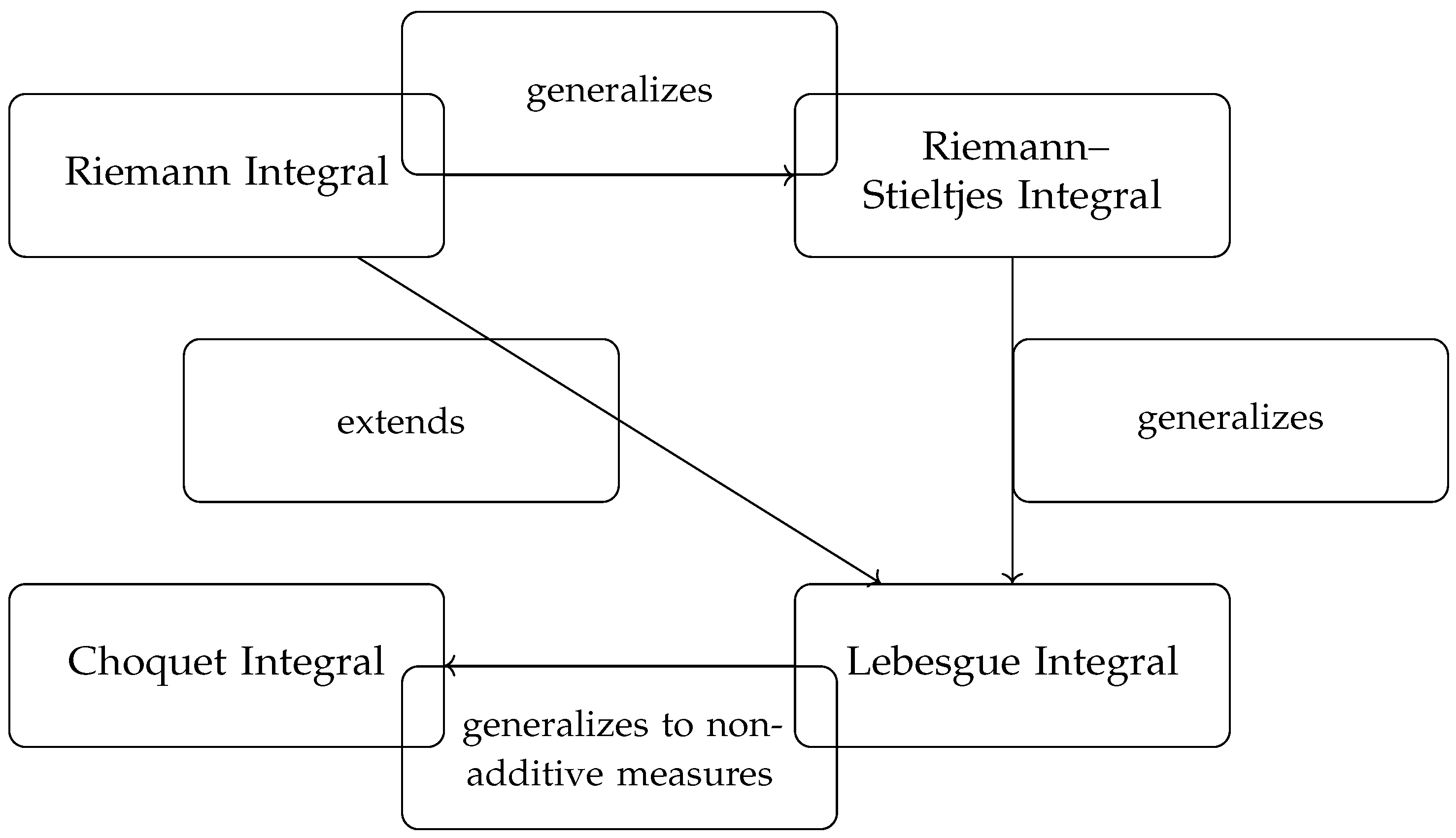
So we can conclude the following:

• The Riemann integral is the classical approach to integration, suitable for well-behaved functions on closed intervals.
• The Riemann–Stieltjes integral generalizes the Riemann integral by integrating with respect to a function $g\left(x\right)$, not just $dx$.
• The Lebesgue integral generalizes both by allowing integration with respect to a measure, offering better convergence properties.
• The Choquet integral generalizes the Lebesgue integral to non-additive measure (capacities), often used in decision theory and fuzzy systems. Having continuity from below will also imply null continuity for a monotonic set function.

Relations among different types of integrals are shown in Figure 1. In the following, we consider examples of monotone set functions defined on algebras. These functions, under suitable conditions, can be extended to countably additive measures.

Our goal is to illustrate how certain set functions—initially defined in a limited context—can give rise to full measures once their additivity and continuity properties are verified.

4. Countable Additivity in Cylinder Set Algebras

In Theorem 2.3 of [14], it has been proved that any finitely additive probability measure defined on the field ${\mathcal{C}}_0$, which encompasses all cylinders in the space of infinite sequences $S^{\infty }$, is, indeed, countably additive. It occurs because any sequence of non-empty cylinders converges from above to a non-empty set, so that there are no sequences converging from above to the empty set, and so Proposition 2.1 is trivially verified.

We recall from Example 3, Remark 1, and Example 4, the construction proposed in [14] (pp. 29–30) because a similar procedure is applied in [12] to prove the countable additivity of the Möbius transform.

Example 5.

Let S be a finite set, and let $\Omega =S^{\infty }$ be the space of all infinite sequences, that is

$$\Omega =\{\omega =(z_1\left(\omega \right),z_2\left(\omega \right),\dots )\}$$

such that $z_k\left(\omega \right)\in S$ for all $\omega \in S^{\infty }$. Consider $S^n$ as the Cartesian product of n copies of the set S. This implies that $S^n$ comprises sequences of length n composed of elements from S,

$$\{\omega :(z_1\left(\omega \right),z_2\left(\omega \right),\dots z_n\left(\omega \right))=u_1,\dots u_n\}.$$

The set represents the event where the first n repetitions of the experiment result in the outcomes $u_1,u_2,\dots ,u_n$ occurring in sequence. For any $H\subset S^n$, a cylinder of rank n is a set of the form

$$A=\{\omega :(z_1\left(\omega \right),z_2\left(\omega \right),\dots z_n\left(\omega \right))\in H\}$$

A cylinder of order n is the set of ω that generates sequences whose first n components are in H. To clarify, for tossing a coin, we have $S=\{0,1\}$, and each $\omega =\left\{(z_1\left(\omega \right),z_2\left(\omega \right),\dots )\right\}$ can be viewed as the result of repeating infinitely often the simple experiment S.

Consider ${\mathcal{C}}_0$ as the field generated by cylinders with all finite ranks. Let $p_u$, where $u\in S$, be a probability distribution defined on S. We can define a probability measure P on ${\mathcal{C}}_0$ such that for a cylinder A, the probability $P\left(A\right)$ is given by

$$P\left(A\right)=\sum _H{p}_{u_1}\dots p_{u_n}.$$

According to Theorem 2.3 of [14], it follows that P is countably additive on ${\mathcal{C}}_0$. The proof of the theorem depends on the fact that if $A_n$ is a sequence of non-empty cylinders converging to A, then A is non-empty since S is a finite set, and in the definition of a cylinder, the set H is non-empty.

A probability can be defined on the field ${\mathcal{C}}_0$ by the product rule and extended to the $\sigma$-field $\mathcal{F}$ generated by the field ${\mathcal{C}}_0$.

In the previous example, a key role in proving that the countable intersection of non-empty cylinders is non-empty is due to the fact that the alphabetic set S is finite.

The result can be generalized when different finite sets $S_K$ of points, regarded as the possible outcomes of a simple experiment, are considered so that each component $z_k\left(\omega \right)\in S_K$.

Example 6.

Theorem 2.3 1 [14] holds even if we consider the space $\Omega =S_1\times S_2\times \dots$ of sequences, where $z_k\left(\omega \right)\in S_k$, and the probability is defined by $P={\sum }_H{p}_{u_1}\dots p_{u_n}$, where the sum extending over all sequences in H is as in Example 3. Moreover, in this case, given any sequence of non-empty cylinders converging from above to a set A, then A is non-empty.

If any of the sets $S_K$ is infinite, it is not assured that for all sequences of non-empty cylinders converging from above to a set A that A is non-empty (see problem 2.20 of [14]).

Example 7.

Let S be a countable set, and let $\Omega =S^{\infty }$ be the space of all infinite sequences, that is

$$\Omega =\{\omega =(z_1\left(\omega \right),z_2\left(\omega \right),\dots )\}$$

such that $z_k\left(\omega \right)\in S$ for all $\omega \in S^{\infty }$. Consider $S^n$ as the Cartesian product of n copies of the set S, and define a cylinder of rank n, as in Example 3

$$A=\{\omega :(z_1\left(\omega \right),z_2\left(\omega \right),\dots z_n\left(\omega \right))\in H\}.$$

Consider ${\mathcal{C}}_0$ as the field generated by cylinders with all having a finite rank. Let $p_u$, where $u\in S$, be a probability distribution defined on S. We can define a probability measure P on ${\mathcal{C}}_0$ such that for a cylinder A, the probability $P\left(A\right)$ is given by

$$P\left(A\right)=\sum _H{p}_{u_1}\dots p_{u_n}.$$

Since S is countable, we can consider a countable quantity of cylinders such that ${\bigcap }_{j=1}^{\infty }{A}_j=\varnothing$ but ${lim}_{n\to \infty }P\left({\bigcap }_{j=1}^n{A}_j\right)\ne 0$.

Remark 1.

We can observe that the approach proposed in Example 2 cannot be applied to define a probability measure in the continuous case. This discrepancy arises due to the relationship between the σ-field $\mathcal{C}$ and the Borel σ-field of the interval $[0,1]$. While the field ${\mathcal{C}}_0$ is smaller than the field ${\mathcal{B}}_0$ of finite disjoint unions of intervals in the range $(0,1]$, there are essential differences between them. One notable distinction is that non-empty sets in ${\mathcal{B}}_0$, such as $\left({\displaystyle \frac{1}{2}},{\displaystyle \frac{1}{2}}+{\displaystyle \frac{1}{2^n}}\right)$, have the potential to contract to the empty set. On the other hand, non-empty sets in ${\mathcal{C}}_0$ do not possess this property. As a result, a finitely additive probability defined on ${\mathcal{B}}_0$ may fail to be countably additive, whereas such a failure cannot occur in ${\mathcal{C}}_0.$

In the following example, we consider a finitely additive but not countably additive probability on the field ${\mathcal{B}}_0$.

Example 8.

Let ${\mathcal{B}}_0$ be the field of finite disjoint unions of intervals in the range $(0,1]$, and let P be a set function defined by

$$P\left(A\right)=\{\begin{array}{ccc}1& \mathit{if}\mathit{exists}& {ϵ}_A:\left({\displaystyle \frac{1}{2}},{\displaystyle \frac{1}{2}}+{ϵ}_A\right]\subset A\\ \\ 0& \mathit{otherwise}\end{array}$$

P is finitely but not countably additive on the σ-field generated by ${\mathcal{B}}_0$ since it is denoted by

$$A_n=\left({\displaystyle \frac{1}{2}},{\displaystyle \frac{1}{2}}+{\displaystyle \frac{1}{n}}\right]$$

and we have ${\displaystyle \underset{n\to \infty }{lim}P\left(A_n\right)=1\ne P\left(\underset{n\to \infty }{lim}{A}_n\right)=0}$.

5. Countably Additive Representation of the Choquet Integral According to the Möbius Transform of a Monotone Set Function of Bounded Variation

Let $\mathcal{A}$ be an algebra of subsets of $\Omega$ properly contained in $\wp (\Omega )$, and let $\nu$ be a coherent lower probability. Let $\mathcal{H}\left(\mathcal{A}\right)$ be the class of all normalized monotone set functions with values in $\left\{0,1\right\}$. Consider the two subsets of $\mathcal{H}\left(\mathcal{A}\right)$

$$H_p\left(A\right)=\left\{\eta \in \mathcal{H}\left(\mathcal{A}\right):\eta \mathrm{supermodalular}\right\}$$

$$H_u\left(A\right)=\left\{u_K\in \mathcal{H}\left(\mathcal{A}\right):K\in \mathcal{A};K\ne \varnothing \right\}$$

where $u_K$ is defined on $\mathcal{A}$ for a fixed K subset of $\Omega$, according to

$$u_K\left(A\right)=\{\begin{array}{ccc}1& \mathrm{if}& K\subset A\\ \\ 0& \mathrm{otherwise}\end{array}$$

In combinatorics, depending on the two variables K and A, $u_K\left(A\right)$ is called the zeta function. It is continuous from above, whereas a general $\left\{0,1\right\}$-valued (even supermodular) set function continuous. $u_K\left(A\right)$ is supermodular, and it is a belief function since it is totally monotone. When $\Omega$ is finite, all filters have the form $\mathcal{A}=\left\{A:A\supset K\right\}$ for some non-empty set K, and so $u_K$ is a coherent lower probability (Section 2.9.8 [22]). In game theory, $u_K$ is called a unanimity game.

Definition 4.

Let $K\subseteq N$ be a coalition. The unanimity game on K is the game $(N,u_K)$ where

$$u_K\left(S\right)=\left\{\begin{array}{cc}1\hfill & \mathit{if}K\subseteq S,\hfill \\ 0\hfill & \mathit{if}K\neg \subseteq S.\hfill \end{array}\right.$$

In other words, a coalition S has a worth of 1 (is winning) if it contains all players of K and a worth of 0 (is losing) if this is not the case.

We have

$$H_u\left(\mathcal{A}\right)\subset H_p\left(\mathcal{A}\right)\subset H\left(\mathcal{A}\right)$$

and the equality $H_u\left(\mathcal{A}\right)=H_p\left(\mathcal{A}\right)$ holds if $\Omega$ is finite.

Let the tilde operator be defined for an $\mathcal{A}$-measurable random variable X and with respect to any $\left\{0,1\right\}$-valued monotone set function $\eta \in \mathcal{H}\left(\mathcal{A}\right)$:

$$\tilde{X}=\int X\left(\omega \right)\eta \left(\omega \right)$$

If X is the indicator function of an event $A\in \mathcal{A}$, then

$$\widetilde{I_A}=I_{\tilde{A}}$$

where $\tilde{A}=\left\{\eta \in \mathcal{H}\left(\mathcal{A}\right):\eta \left(A\right)=1\right\}$.

Though $\mathcal{A}$ is a field, the set system $\tilde{\mathcal{A}}=\left\{\tilde{A}|A\in \mathcal{A}\right\}$ is not a field in $\wp \left(\mathcal{H}\right(\mathcal{A}\left)\right)$, except for the trivial case $\tilde{A}=\left\{\varnothing ,\Omega \right\}$.

We consider the field $\mathcal{D}\left(\tilde{\mathcal{A}}\right)$ generated by $\tilde{\mathcal{A}}$ that is the smallest field containing $\tilde{\mathcal{A}}$.

If $(\Omega ,\mathcal{F})$ is a measurable space and $\varnothing \ne E\subseteq \Omega$, then $\left\{E\cap A:A\in \mathcal{F}\right\}$ is a $\sigma$-field on E called the $\mathit{trace}$$-field.$

Let ${\mathcal{D}}^{\prime }\left(\tilde{\mathcal{A}}\right)$ and ${\mathcal{D}}^{″}\left(\tilde{\mathcal{A}}\right)$ be the trace $\sigma$ fields generated by $\tilde{A}$, respectively, in $H_p\left(A\right)$ and $H_u\left(A\right).$

Definition 5.

Given a monotone set function ν on $\mathcal{A}$, the additive Möbius transform ${\mu }^{\nu }$ is uniquely determined on $(H_u\left(A\right),{\mathcal{D}}^{″}\left(\tilde{\mathcal{A}}\right))$ by

$${\mu }^{\nu }\left(\tilde{A}\right)=\nu \left(A\right)\mathit{for}A\in \mathcal{A}.$$

Moreover, in [12], it is proven that integrals are preserved under the Möbius transform, i.e.,

$$\int Xd\nu =\int \tilde{X}d{\mu }^{\nu }$$

Example 9.

For a fixed non-empty set $K\in \wp (\Omega )$, the Choquet integral with respect to the set function $u_K$ on $\wp (\Omega )$ is

$$\tilde{X}=\int X\left(\omega \right)d{u}_K\left(\omega \right)=\underset{\omega \in K}{inf}X\left(\omega \right);$$

and the integral with respect to the restriction of $u_K$ to a field $\mathcal{A}$ of an $\mathcal{A}$-measurable random variable X is

$$\tilde{X}=\int X\left(\omega \right)d{u}_K\left(\omega \right)=\underset{\omega \in K}{inf}X\left(\omega \right)$$

even if K does not belong to $\mathcal{A}$.

The Möbius transform of the monotone set function $u_K$ is defined by ${\mu }^{u_K}\left(\tilde{A}\right)=u_K\left(A\right)$.

A set function $\nu$ on an algebra $\mathcal{A}\subset \wp (\Omega )$ is totally monotone if and only if its Möbius transform ${\mu }^{\nu }$ is monotone, i.e., non-negative [23,24].

In Theorem 6.2 of [12], the following result has been proved

Theorem 1.

If $\nu \in V_b\left(\mathcal{A}\right)$, the Möbius transform ${\mu }^{\nu }$ can be uniquely extended to $(H_p\left(A\right),D^{\prime }\left(\tilde{A}\right))$, and it is σ-additive and named the σ-additive Möbius transform of ν. It is a signed (i.e., it can assume real negative values) additive set function.

The $\sigma$-additivity of the Möbius transform ${\mu }^{\nu }$ on $(H_p\left(A\right),D^{\prime }\left(\tilde{A}\right))$ is satisfied because ${\mu }^{\nu }$ is finite additive and continuous from above to the empty set, and so, according Proposition 1, it is countably additive. Continuity from above to the empty set holds because for any ${\mathcal{D}}_n\in {\mathcal{D}}^{\prime }\left(\tilde{\mathcal{A}}\right)$ such that ${\mathcal{D}}_n\downarrow \varnothing$, there exist $\overline{n}\in \mathbb{N}$ such that ${\mathcal{D}}_n=\varnothing$ for $n>\overline{n}$ (Lemma 6.1 of [12]). It implies that ${\bigcap }_n{\mathcal{D}}_n=\varnothing$. Theorem 3 holds because this lemma guarantees that the intersection of each decreasing sequence ${\mathcal{D}}_n$ is equal to the empty set so that any monotone set function defined on ${\mathcal{D}}^{\prime }\left(\tilde{\mathcal{A}}\right)$ trivially is continuous from above to the empty set, and every finitely additive function is $\sigma$-additive (see Proposition 1).

Lemma 6.1 of [12] is proven by contradiction. It is proven that if we assume $D_n\ne \varnothing$ for large n, then it is possible to construct a sequence $E_n$, with $E_n\ne \varnothing$ for all n, such that there exists a set function $\eta \in {\mathcal{H}}^{\prime }$ with $\eta \in {\bigcap }_n{E}_n$ so that we get the contradiction that $E_n\downarrow \varnothing$.

In Theorem 2.3 of [14], instead, every finitely additive probability is proven to be countably additive because any sequence of non-empty cylinders converges from above to a non-empty set so that there are no sequences converging, from above to the empty set, and so Proposition 1 is trivially verified.

We can observe that the finite probability P in Example 5 is not continuous from above to the empty set since $A_n\downarrow \varnothing$ but ${lim}_{n\to \infty }P\left(A_n\right)=1\ne 0$. So P is finitely additive but not countably additive.

We can observe that the unanimity game $u_K$ cannot be used in Theorems 1 and 2 to define coherent upper conditional previsions and probability because it is not finitely additive.

The following example [12] shows that Möbius transforms can differ on the two measurable spaces $(H_p,{\mathcal{D}}^{\prime }\left(\tilde{\mathcal{A}}\right))$ and $(H_u,{\mathcal{D}}^{\prime \prime }\left(\tilde{\mathcal{A}}\right))$.

Example 10.

Let ${\mu }^{\nu }$ be the Möbius transform defined on ${\mathcal{D}}^{\prime }\left(\tilde{\mathcal{A}}\right)$ of the probability $\nu =P$ of Example 8, that is,

$${\mu }^{\nu }\left(D\right)=\{\begin{array}{cccc}1& \mathit{if}\mathit{exists}& \widetilde{A_n}\subset D& \mathit{for}\mathit{some}\mathrm{n},\\ \\ 0& \mathit{otherwise}\end{array}$$

We can observe that ν does not belong to $H_u$, that is, ν is not an unanimity game $u_K$ for fixed K. The Möbius transform is the Dirac measure at the point $\eta =\nu$ on the measurable space $(H_p,{\mathcal{D}}^{\prime }\left(\tilde{\mathcal{A}}\right))$, and it is continuous from above, contrary to ${\mu }^{\nu }$ on $(H_u,{\mathcal{D}}^{″}\left(\tilde{\mathcal{A}}\right))$ and ν. This can happen since, in $H_p$, we have $\nu \in {\bigcap }_{n=1}^{\infty }\tilde{A}$ so that any sequence ${\tilde{A}}_n$ does not converge to the empty set.

6. Hausdorff Outer Measure-Based Framework for Coherent Upper Conditional Previsions

Let $\mathbf{B}$ be a partition of a metric space $(\Omega ,d)$. A bounded random variable is a function $X:\Omega \to \mathbb{R}$, where $\mathbb{R}=(-\infty ,+\infty )$ denotes the real numbers. Let $L(\Omega )$ denote the set of all such bounded real-valued functions defined on $\Omega$.

For each element $B\in \mathbf{B}$, we denote by ${X|}_B$ the restriction of the random variable X to the set B. The supremum of X over B is denoted by $sup\left(X{|}_B\right)$, i.e., the least upper bound of the values that X takes on B. We define $L\left(B\right)$ as the collection of all bounded random variables restricted to B.

Given a subset $A\subseteq B$, the indicator function $I_A:B\to \{0,1\}$ is defined by

$$I_A\left(\omega \right)=\left\{\begin{array}{cc}1\hfill & \mathrm{if}\omega \in A,\hfill \\ 0\hfill & \mathrm{if}\omega \notin A.\hfill \end{array}\right.$$

For every $B\in \mathbf{B}$, we consider coherent upper conditional expectations (also known as coherent upper conditional previsions) $\overline{P}(·|B)$, which are real-valued functionals defined on $L\left(B\right)$ [22].

Definition 6.

A functional $\overline{P}(·|B):L\left(B\right)\to \mathbb{R}$ is called a coherent upper conditional prevision if, for all $X,Y\in L\left(B\right)$ and every constant $\lambda >0$, the following conditions hold:

1. 

$\overline{P}\left(X\right|B)\le sup\left(X\right|B)$;

2. 

$\begin{array}{cc}\overline{P}\left(\lambda X\right|B)=\lambda \overline{P}\left(X\right|B)\hfill & \hfill \hspace{1em}\hspace{1em}\hspace{1em}\hspace{1em}\hspace{1em}\hspace{1em}\hspace{1em}\hspace{1em}\hspace{1em}\hspace{1em}\hspace{1em}\hspace{1em}\hspace{1em}\hspace{1em}\left(\mathit{positive\; homogeneity}\right);\end{array}$

3. 

$\begin{array}{cc}\overline{P}(X+Y|B)\le \overline{P}\left(X\right|B)+\overline{P}\left(Y\right|B)\hfill & \hfill \hspace{1em}\hspace{1em}\hspace{1em}\hspace{1em}\hspace{1em}\hspace{1em}\hspace{1em}\hspace{1em}\hspace{1em}\hspace{1em}\hspace{1em}\hspace{1em}\left(\mathit{sub-additivity}\right).\end{array}$

A novel framework for defining coherent upper previsions has been proposed based on the Choquet integral with respect to Hausdorff outer measures. This approach provides a rich and flexible method for modeling upper expectations in settings with imprecise or non-additive probabilities.

6.1. Hausdorff Outer Measures

In this section sub-additive Hausdorff outer measures [25], [26] are recalled.

Let ($\Omega ,d)$ be a metric space. The diameter of a non-empty set U of $\Omega$ is defined as $\left|U\right|=sup\left\{d(x,y):x,y\in U\right\}$, and if a subset A of $\Omega$ is such that $A\subset {\bigcup }_i{U}_i$ and $0<$$\left|U_i\right|<\delta$ for each i, the class $\left\{U_i\right\}$ is called a $\delta$-cover of A. Let s be a non-negative number. For $\delta >0$, we define ${\mathcal{H}}_{s,\delta }\left(A\right)=inf{\sum }_{i=1}^{\infty }{\left|U_i\right|}^s$, where the infimum is over all $\delta$-covers $\left\{U_i\right\}$. The Hausdorff s-dimensional outer measure of A [25,26], denoted by ${\mathcal{H}}^s\left(A\right)$, is defined as

$${\mathcal{H}}^s\left(A\right)=li{m}_{\delta \to 0}{\mathcal{H}}_{s,\delta }\left(A\right).$$

This limit exists but may be infinite since $\mathcal{H}s,\delta \left(A\right)$ increases as $\delta$ decreases. The s-dimensional Hausdorff outer measure is submodular and continuous from below.

The property of being a metric outer measure ensures that if sets E and F are positively separated (i.e., $d(E,F)=inf\left\{d\right(x,y):x\in E,y\in F\}>0$), then

$${\mathcal{H}}^s(E\cup F)={\mathcal{H}}^s\left(E\right)+{\mathcal{H}}^s\left(F\right).$$

According to Falconer’s Theorem 1.5 [25], as Hausdorff outer measures are metric outer measures, all Borel subsets of $\Omega$ are measurable.

The Hausdorff dimension of a set A, $di{m}_H\left(A\right)$, is defined as the unique value, such that

$$\begin{array}{c}{\mathcal{H}}^s\left(A\right)=\infty \mathrm{if}0\le s<di{m}_H\left(A\right),\\ {\mathcal{H}}^s\left(A\right)=0\mathrm{if}di{m}_H\left(A\right)<s<\infty .\end{array}$$

6.2. Hausdorff Measures and Bounded Variation Functions

A set $E\subset {\mathbb{R}}^n$ is said to be m-rectifiable if there exist countably many Lipschitz functions

$$f_i:{\mathbb{R}}^m\to {\mathbb{R}}^n,i\in \mathbb{N},$$

such that

$${\mathcal{H}}^m\left(E\setminus \bigcup _{i=1}^{\infty }{f}_i\left({\mathbb{R}}^m\right)\right)=0$$

where ${\mathcal{H}}^m$ denotes the m-dimensional Hausdorff measure.

Let $u\in L^1\left({\mathbb{R}}^n\right)$. We say that the distributional derivative $Du$ of u defines a (vector-valued) Radon measure $\mu$ on ${\mathbb{R}}^n$ if for every test function, $\phi \in C_c^{\infty }({\mathbb{R}}^n;{\mathbb{R}}^n)$,

$${\int }_{{\mathbb{R}}^n}u\mathrm{div}\phi dx=-{\int }_{{\mathbb{R}}^n}\phi ·d\mu .$$

In this case, we write $Du=\mu$ in the sense of distributions, and $\mu$ is called the distributional (or weak) derivative of u.

A set $E\subset {\mathbb{R}}^n$ is said to be purely m-unrectifiable if for every Lipschitz map $f:{\mathbb{R}}^m\to {\mathbb{R}}^n$, the m-dimensional Hausdorff measure of $E\cap f\left({\mathbb{R}}^m\right)$ is zero:

$${\mathcal{H}}^m(E\cap f\left({\mathbb{R}}^m\right))=0.$$

In other words, E does not contain any subset of positive ${\mathcal{H}}^m$-measure that is m-rectifiable.

In general, the s-dimensional Hausdorff measure ${\mathcal{H}}^s$ (for $0<s<n$) on ${\mathbb{R}}^n$ cannot be derived from a function of bounded variation. That is, ${\mathcal{H}}^s$ is not a Lebesgue–Stieltjes measure associated with any real-valued function of bounded variation on ${\mathbb{R}}^n$.

Recall that a function $f:{\mathbb{R}}^n\to \mathbb{R}$ of bounded variation (i.e., $f\in BV\left({\mathbb{R}}^n\right)$) defines a Radon measure ${\mu }_f$ via distributional derivatives. The measure ${\mu }_f$ is supported on countably $(n-1)$-rectifiable sets and satisfies the following:

• It is absolutely continuous with respect to the $(n-1)$-dimensional Hausdorff measure ${\mathcal{H}}^{n-1}$;
• It gives zero measure to purely unrectifiable sets (such as the classic Cantor set or many fractals).

However, many Hausdorff measures ${\mathcal{H}}^s$ (for $0<s<n-1$) assign positive measure to purely unrectifiable sets, which contradicts the behavior of measures derived from BV functions.

Hence, no such f can exist, and ${\mathcal{H}}^s$ is not the distributional derivative of a function of bounded variation.

Example 11.

Let $C\subset [0,1]$ denote the classic middle-third Cantor set. It is totally disconnected and nowhere dense. It has zero Lebesgue measure and has a positive ${\mathcal{H}}^s$ measure for $s=log2/log3$.

Since C is purely unrectifiable, no BV function f can generate a measure ${\mu }_f$ such that ${\mu }_f\left(C\right)>0$. Therefore, ${\mathcal{H}}^s{|}_C$ is not a BV-derived measure.

Example 12.

The von Koch snowflake curve is a fractal in ${\mathbb{R}}^2$ with a finite ${\mathcal{H}}^s$ measure for some $s>1$, but it is nowhere differentiable and purely unrectifiable. Again, any BV function-derived measure must be concentrated on rectifiable sets, so it cannot capture ${\mathcal{H}}^s$ on the Koch curve.

Hausdorff measures ${\mathcal{H}}^s$ with $s\notin \mathbb{N}$, especially when $s<n-1$ cannot be represented as distributional derivatives of functions of bounded variation. This is due to the fundamental difference in their support: BV-derived measures are concentrated on rectifiable sets, whereas Hausdorff measures can give full measure to purely unrectifiable sets.

Theorem 2.

Let ${\mathcal{H}}^s$ denote the s-dimensional Hausdorff outer measure on ${\mathbb{R}}^n$, with $s>0$. Then, ${\mathcal{H}}^s$ is not, in general, derived from a function of bounded variation. In particular, there does not exist a function $F:{\mathbb{R}}^n\to \mathbb{R}$ of bounded variation such that ${\mathcal{H}}^s\left(E\right)={\int }_{E}dF$ for all Borel sets $E\subseteq {\mathbb{R}}^n$.

Proof. 

Suppose, for contradiction, that ${\mathcal{H}}^s$ is derived from a function F of bounded variation on ${\mathbb{R}}^n$. Then, by the Riesz Representation Theorem, ${\mathcal{H}}^s$ would define a finite Radon measure on compact subsets of ${\mathbb{R}}^n$, and in particular, would be regular and finite on all compact sets.

However, this contradicts the behavior of ${\mathcal{H}}^s$ for many sets of positive s-dimensional measure. For example, let $C\subseteq [0,1]$ be the standard middle-third Cantor set. It is known that C has Hausdorff dimension $log2/log3$, and its Hausdorff measure ${\mathcal{H}}^s\left(C\right)$ is finite and positive when $s=log2/log3$. □

6.3. Countably Additive Coherent Conditional Probability

We recall the model of conditional upper prevision based on Hausdorff outer measures, as introduced in [27,28,29]. In this framework, the conditional upper probability, which typically represents the probability of an event occurring, given that another is defined using the Hausdorff outer measure of order s, also known as the s-dimensional Hausdorff measure, when the conditioning event has a Hausdorff dimension equal to s.

Theorem 3.

Let $(\Omega ,d)$ be a metric space, and let B  be a partition of Ω. For every $B\in \mathit{B}$ denote by s the Hausdorff dimension of the conditioning event B and by ${\mathcal{H}}^s$ the Hausdorff s-dimensional outer measure. Let $m_B$ be a 0-1-valued, finitely additive, but not countably additive, probability on $\wp \left(B\right)$. Then, for each $B\in \mathit{B}$, the functional $\overline{P}\left(X\right|B)$ defined on $L\left(B\right)$ by

$$\overline{P}\left(X\right|B)=\{\begin{array}{ccc}{\displaystyle \frac{1}{{\mathcal{H}}^s\left(B\right)}}{\int }_{B}Xd{h}^s& if& 0<{\mathcal{H}}^s\left(B\right)<+\infty \\ {\int }_{B}Xd{m}_B& if& {\mathcal{H}}^s\left(B\right)\in \left\{0,+\infty \right\}\end{array}$$

is a coherent upper conditional probability.

The restriction to the class of all indicator functions of the coherent upper conditional prevision in Theorem 1 is the following coherent upper conditional probability:

Theorem 4.

Let $(\Omega ,d)$ be a metric space, and let  B  be a partition of Ω. For every $B\in \mathit{B}$, denote by s the Hausdorff dimension of the conditioning event B and by ${\mathcal{H}}^s$ the Hausdorff s-dimensional outer measure. Let $m_B$ be a 0-1-valued, finitely additive, but not countably additive, probability on $\wp \left(B\right)$. Then, for each $B\in \mathit{B}$, the functional $\overline{P}\left(A\right|B)$ defined on $\wp \left(B\right)$ by

$$\overline{P}\left(X\right|B)=\{\begin{array}{ccc}{\displaystyle \frac{{\mathcal{H}}^s(A\cap B)}{{\mathcal{H}}^s\left(B\right)}}& if& 0<{\mathcal{H}}^s\left(B\right)<+\infty \\ m_B& if& {\mathcal{H}}^s\left(B\right)\in \left\{0,+\infty \right\}\end{array}$$

is a coherent upper conditional probability.

Let us consider a set $B\in \mathbf{B}$ with a positive and finite Hausdorff outer measure corresponding to its Hausdorff dimension s. In this scenario, we define the monotone set function ${\mu }_B^{*}$ for every $A\in \wp \left(B\right)$ as follows: ${\mu }_B^{*}\left(A\right)={\displaystyle \frac{{\mathcal{H}}^s\left(AB\right)}{{\mathcal{H}}^s\left(B\right)}}$. This function serves as a coherent upper conditional probability and exhibits properties such as submodularity and continuity from below. Furthermore, when we restrict it to the $\sigma$-field of all ${\mu }_B^{*}$-measurable sets, it becomes a Borel regular countably additive probability. When considering $B\in \mathbf{B}$ such that ${\mathcal{H}}^s\left(B\right)$ falls within the set $\left\{0,+\infty \right\}$, the consistent upper conditional probability is established through a finitely additive probability $m_B$ on $\wp \left(B\right)$, which takes values of either 0 or 1 and is not countably additive. Notably, the realm of 0–1-valued, finitely additive probabilities is in direct bijective correspondence with ultrafilters, as outlined in the context of $\mathcal{A}$.

7. On the Continuity of Coherent Conditional Upper Previsions Induced by Hausdorff Measures

The $\sigma$-additive Möbius transform of a real supermodular monotone set function $\nu \in V_b\left(\mathcal{F}\right)$ is considered to define coherent conditional probability when the conditioning event has a Hausdorff measure in its Hausdorff dimension equal to zero or infinity.

In the following theorem, a coherent countably additive conditional probability is defined on the Borel $\sigma$-field.

Theorem 5.

Let $(\Omega ,d)$ be a metric space, and let $\mathcal{F}$ be the Borel σ-field. Let  B  be a Borel partition of Ω. For every $B\in \mathit{B}$, denote by s the Hausdorff dimension of the conditioning event B and by ${\mathcal{H}}^s$ the Hausdorff s-dimensional outer measure. Let ${\mu }^{\nu }$ be the σ-additive Möbius transform of a finite additive probability $\nu \in V_b\left(\mathcal{F}\right)$. Thus, for each $B\in \mathit{B}$, the function defined on $\mathcal{F}$ by

$$\overline{P}\left(A\right|B)=\{\begin{array}{ccc}{\displaystyle \frac{{\mathcal{H}}^s(A\cap B)}{{\mathcal{H}}^s\left(B\right)}}& if& 0<{\mathcal{H}}^s\left(B\right)<+\infty \\ {\mu }_{\tilde{B}}^{\nu }\left(\tilde{A}\right)& if& {\mathcal{H}}^s\left(B\right)\in \left\{0,+\infty \right\}\end{array}$$

is a coherent σ-additive conditional probability.

Proof. 

If $0<{\mathcal{H}}^s\left(B\right)<+\infty$, the coherence of $\overline{P}\left(A\right|B)$ is proven in [28]. If ${\mathcal{H}}^s\left(B\right)\in \left\{0,+\infty \right\}$$\overline{P}\left(A\right|B)$, it is a coherent conditional probability since it is countably additive, and the condition $\overline{P}\left(B\right|B)=1$ is satisfied because (see Proposition 3.1 and Example 7.1 of [12])

$${\displaystyle \frac{{\mu }^{\nu }(\tilde{A}\cap \tilde{B})}{{\mu }^{\nu }\left(\tilde{B}\right)}}={\displaystyle \frac{{\mu }^{\nu }\left(\widetilde{A\cap B}\right)}{{\mu }^{\nu }\left(\tilde{B}\right)}}={\displaystyle \frac{\nu (A\cap B)}{\nu \left(B\right)}}.$$

(1)

□

Remark 2.

According to Theorem 6.2 of [12], if the additive probability is $\nu \in V_b\left(\mathcal{F}\right)$, then there is a unique σ-additive Möbius transform.

Example 13.

Let $(\Omega ,d)$ be a metric space, and let $\mathcal{F}$ be the Borel σ-field. Let  B  be a Borel partition of Ω. For every $B\in \mathit{B}$, denote by s the Hausdorff dimension of the conditioning event B and by ${\mathcal{H}}^s$ the Hausdorff s-dimensional outer measure. Let ${\mu }^{\nu }$ be the σ-additive Möbius transform defined on ${\mathcal{D}}^{\prime }$ (see Example 6) of the additive function ν of Example 4

$${\mu }^{\nu }\left(D\right)=\{\begin{array}{cccc}1& \mathit{if}\mathit{exists}& \widetilde{A_n}\subset D& \mathit{for}\mathit{some}\mathrm{n},\\ \\ 0& \mathit{otherwise}\end{array}$$

Then, the coherent conditional probability defined on $\mathcal{F}$ by

$$\overline{P}\left(A\right|B)=\{\begin{array}{ccc}{\displaystyle \frac{{\mathcal{H}}^s(A\cap B)}{{\mathcal{H}}^s\left(B\right)}}& if& 0<{\mathcal{H}}^s\left(B\right)<+\infty \\ {\mu }_{\tilde{B}}^{\nu }\left(\tilde{A}\right)& if& {\mathcal{H}}^s\left(B\right)\in \left\{0,+\infty \right\}\end{array}$$

is a coherent σ-additive conditional probability.

The model proposed in Theorem 5 can be used to assign a countably additive probability in the sequence space recalled in Example 4 when S is countable or, in Example 2, when at least one of the alphabetic sets $S_k$ is infinite.

In [19], the monotone convergence theorem is proven for a monotone set function.

Theorem 6

(Monotone Convergence Theorem). Let μ be a monotone set function on a σ-field F properly contained in $\wp (\Omega$), which is continuous from below. For an increasing sequence of non-negative, F-measurable random variables $X_n$, the limit function $X=li{m}_{n\to \infty }{X}_n$ is F-measurable and $li{m}_{n\to \infty }\int X_{n}d\mu =\int Xd\mu$.

Remark 3.

It is not restrictive to consider this in the monotone convergence theorem sequence of non-negative random variables, as any random variable X can be decomposed in its positive part $X^{+}$, and its negative part $X^{-}$ given by

$$X=X^{+}-X^{-};X^{+}=0\vee X;X^{-}={(-X)}^{+}$$

where ∨ is the maximum.

Theorem 7.

Let $(\Omega ,d)$ be a metric space, and let  B  be a partition of Ω. For every $B\in \mathit{B}$, denote by s the Hausdorff dimension of the conditioning event B and by ${\mathcal{H}}^s$ the s-dimensional Hausdorff outer measure. Let $\mathit{F}$ be the σ-field of $h^s$-measurable sets, and let $\mathit{K}$ be the class of all $\mathit{F}$-measurable random variables. If B has a positive and finite Hausdorff outer measure in its dimension, then the functional defined as in Theorem 1 is continuous from below; that is, given an increasing sequence of non-negative random variables $X_n$ of  K  converging point-wise to the random variable X, we have it that $li{m}_{n\to \infty }\overline{P}\left(Xn\right|B)=\overline{P}\left(X\right|B)$.

Proof. 

If the set B has a positive and finite Hausdorff outer measure in its Hausdorff dimension s, then the conditional upper prevision is given by

$$\overline{P}(X\mid B)={\displaystyle \frac{1}{{\mathcal{H}}^s\left(B\right)}}{\int }_{B}Xd{\mathcal{H}}^s.$$

Since the s-dimensional Hausdorff outer measure is continuous from below, the monotone convergence theorem implies that the conditional upper prevision $\overline{P}(X\mid B)$ is also continuous from below. That is,

$$li{m}_{n\to \infty }\overline{P}\left(Xn\right|B)=li{m}_{n\to \infty }{\displaystyle \frac{1}{{\mathcal{H}}^s\left(B\right)}}{\int }_B{X}_{n}d{\mathcal{H}}^s={\displaystyle \frac{1}{{\mathcal{H}}^s\left(B\right)}}{\int }_{B}Xd{\mathcal{H}}^s=\overline{P}\left(X\right|B).$$

□

Theorem 8.

Let μ be a null-continuous monotone set function, and let $X_n$ be an increasing sequence of functions converging to X, $X_n\uparrow X$ such that $X_n=0$ μ a.e.; then, we have it that $li{m}_{n\to \infty }\overline{P}\left(Xn\right|B)=\overline{P}\left(X\right|B)$.

In the following theorems, we consider the extension to the class of Borel measurable random variables of the countably additive conditional probability defined in Theorem 5; we prove that these extensions are continuous, linear previsions for each conditioning event B if the real monotone set function $\nu \in V_b\left(\mathcal{F}\right)$ is countably additive.

Theorem 9.

If $\nu \in V_b\left(\mathcal{F}\right)$ is a real coherent lower probability that is not continuous from below, then the functional defined by

$$\underline{P}\left(X\right|B)={\int }_{\tilde{B}}\tilde{X}d{\mu }_{\tilde{B}}^{\nu }$$

if ${\mathcal{H}}^s\left(B\right)\in \left\{0,+\infty \right\}$ is a coherent lower conditional prevision that is not continuous.

Proof. 

Since [12] the Choquet integrals are preserved under the Möbius transform, we have

$${\int }_{B}Xd\nu ={\int }_{\tilde{B}}\tilde{X}d{\mu }^{\nu }$$

and if $\nu$ is not continuous from below, then according to Theorem 8, we have it that the functional $\underline{P}\left(X\right|B)$ is not continuous. □

According to the previous theorems, we have

Theorem 10.

Let $(\Omega ,d)$ be a metric space, and let $\mathcal{F}$ be the Borel σ-field. Let  B  be a partition of Ω. For every $B\in \mathit{B}$, denote by s the Hausdorff dimension of the conditioning event B and by ${\mathcal{H}}^s$ the Hausdorff s-dimensional outer measure. Let ${\mu }^{\nu }$ be the σ-additive Möbius transform of a finitely additive conditional probability ν of bounded variation. Then, for each $B\in \mathit{B}$ with a positive and finite Hausdorff s-dimensional outer measure, the functional $\overline{P}\left(X\right|B)$ is defined on the class of all $\mathcal{F}$-measurable random variables by

$$\overline{P}\left(X\right|B)=\{\begin{array}{ccc}{\displaystyle \frac{1}{{\mathcal{H}}^s\left(B\right)}}{\int }_{B}Xd{\mathcal{H}}^s& if& 0<{\mathcal{H}}^s\left(B\right)<+\infty \\ {\int }_{\tilde{B}}\tilde{X}d{\mu }_{\tilde{B}}^{\nu }& if& {\mathcal{H}}^s\left(B\right)\in \left\{0,+\infty \right\}\end{array}$$

is a continuous linear conditional prevision.

It is important to observe that Theorem 8 holds because bounded random variables are considered. Extensions to unbounded random variables are investigated in [29].

Example 14.

Let Ω be an uncountable set and fixed $a\in \Omega$, and define the countable additive probability on the Borel σ-field by

$$\nu \left(A\right)=\{\begin{array}{cccc}1& \mathit{if}& a\in A& ,\\ \\ 0& \mathit{otherwise}\end{array}$$

Then, $\tilde{X}\left(\nu \right)=X\left(a\right)$ and since

$${\int }_{B}Xd\nu ={\int }_{\tilde{B}}\tilde{X}d{\mu }^{\nu },$$

then the Möbius transform is

$${\mu }_{\tilde{B}}^{\nu }\left(\tilde{A}\right)=\{\begin{array}{cccc}1& \mathit{if}& a\in A& \\ \\ 0& \mathit{otherwise}\end{array}$$

Example 15.

Let the field ${\mathcal{B}}_0$ and the additive probability $\nu =P$ be as in Example 8, and consider the partition $\mathit{B}=\left\{(0,{\displaystyle \frac{1}{4}}];({\displaystyle \frac{1}{4}},1]\right\}$. We have it that $P\left(0,{\displaystyle \frac{1}{4}}\right]=0$ and $P\left({\displaystyle \frac{1}{4}},1\right]=1$.

The Choquet integral representation of the extension of P to the class of all bounded random variables by the σ-additive Möbius transform ${\mu }^{\nu }$ of Example 8 does not satisfy the monotone convergence theorem because $\nu =P$ is not continuous from below.

If the monotone set function ν is defined by a Hausdorff outer measure, as in Theorem 7, we have it that $\nu \left(A\right|B)=P\left(A\right|B)={\displaystyle \frac{{\mathcal{H}}^1(A\cap B)}{h^1\left(B\right)}}$ since all sets in the partition $\mathit{B}$ has a Hausdorff dimension equal to 1 and $\nu \left(A\right)={\displaystyle \frac{{\mathcal{H}}^1\left(A\right)}{{\mathcal{H}}^1(\Omega )}}$. The outer Hausdorff measures are continuous from below (Lemma 1.3 [25]), so the monotone convergence theorem can be applied, and the extensions $P\left(X\right|B)$ and $P\left(X\right|\Omega )$ are continuous.

It is important to note that if the conditioning event has a Hausdorff measure in its Hausdorff dimension equal to zero, but it has a positive and finite packing measure in the same dimension (see Example 6 of [30]), we can define coherent upper previsions according to the packing outer measure; this outer measure is continuous from below, and it is a metric outer measure such that it is a measure on the Borel $\sigma$-field; this means that the monotone convergence theorem holds and the coherent previsions defined as in Theorem 6 are continuous. For this reason, other fractal outer measures have been introduced and investigated in [31,32,33].

Otherwise, if the conditioning event has a Hausdorff outer measure equal to infinity, as occurs if it is countable (see Example 8 in [30]), then to define a coherent conditional prevision, we have to consider the $\sigma$-additive Möbius transform of a 0–1-valued, finitely additive probability.

7.1. Weak Monotone Convergence Theorem

A sequence of random variables satisfies the weak monotone convergence theorem (WMCT) with respect to a monotone set function $\mu$ if the monotone convergence theorem is satisfied for sequences of random variables that are equal to zero almost everywhere with respect to $\mu$

Theorem 11.

(WMCT) Let μ be a monotone set function on $\wp (\Omega )$, and let $X_n$ be a sequence such that $X_n=0$ μ, a.e., $\forall n\in \mathcal{N}$ and $X_n\uparrow X$, then ${lim}_{n\to \infty }\int X_{n}d\mu =\int Xd\mu$.

Theorem 12.

(WMCT) Let μ be a null-continuous monotone set function on $\wp (\Omega )$, and let $X_n$ be a sequence such that $X_n=0$ μ, a.e., $\forall n\in \mathcal{N}$ and $X_n\uparrow X$, then the weak monotone convergence theorem holds.

Proof. 

According to Proposition 5 and Proposition 11 of [21], we have it that $X=0$ $\mu$, a.e., and $\int Xd\mu =0.$ □

7.2. Theoretical Contributions

In this subsection, the findings are contextualized within the broader mathematical literature so as to state, in evidence, their novelty and impact. The key points include the following:

• Advancement of integration theory through countably additive representation: The paper introduces a countably additive representation of the Choquet integral, which significantly advances existing integration theory. This representation enables a linear extension of a coherent upper prevision via a conditional probability under the condition that the conditioning event has a positive and finite Hausdorff outer measure in its Hausdorff dimension. This result relies on the metric and outer regular nature of Hausdorff outer measures, which ensures that every Borel set is measurable with respect to them.
• Handling of degenerate conditioning events: The proposed model offers a novel method to update partial knowledge, even when the conditioning event is unexpected or degenerate. This is achieved by employing the Hausdorff measure of the conditioning event’s dimension to define the conditional probability, thereby enabling coherent updating in cases where traditional approaches fail.
• σ-additive Möbius transforms and coherent conditional previsions: The use of $\sigma$-additive Möbius transforms is shown to play a crucial role in constructing coherent conditional previsions. This enriches the theory of imprecise probabilities by bridging Möbius transforms with the structural properties of coherent assessments under uncertainty [17,18]. A future aim of this research is to investigate the optimal transport control of two monotone set functions by using the representation of the Choquet integral by the countably additive Möbius transform. The transport problem has been formulated in terms of Möbius transform for non-additive measures, and in the finite case in [34], for a lower probability, which is the lower envelope of a particular type of credal sets (convex and weak*-closed set) [35], and for belief functions [36,37].
• Connections to capacities and outer measures: The results establish new connections and significant departures from foundational work on capacities and outer measures. In particular, the framework allows for a deeper understanding of the properties of monotone set functions, facilitating the selection of appropriate monotone functions based on specific modeling objectives.

8. Conclusions

In this work, we have addressed the problem of representing the Choquet integral with respect to a monotone set function—specifically, a Hausdorff outer measure that is not necessarily derived from a function of bounded variation—by means of a countably additive measure defined on suitable domains. We have shown that such a representation is indeed possible, thereby establishing a bridge between non-additive integration and classical measure theory.

A key contribution is the construction of a countably additive measure that coincides with the Choquet integral on a sufficiently rich class of integrable functions, despite the non-additivity of the original capacity. This construction is based on the continuity from below of Hausdorff outer measures and on identifying appropriate domains on which the additivity of the integral can be recovered.

Moreover, we have considered the countably additive Möbius transform associated with a monotone set function of bounded variation in order to define a coherent, countably additive conditional prevision. This framework is applicable, even when the conditioning event has a Hausdorff measure in its own dimension equal to zero or infinity—cases which are typically problematic within standard measure-theoretic conditioning. Coherent, countably additive conditional probabilities within a metric space framework are defined using the dimensional Hausdorff measures on the Borel $\sigma$-algebra. We demonstrated that when the conditioning event has a positive and finite s-Hausdorff measure, the conditional probability can be directly defined using this measure. When these conditions are not met, instead, we define the conditional probability through the $\sigma$-additive Möbius transform of a 0–1-valued, finitely additive probability of bounded variation.

We further extended our framework to include all Borel-measurable random variables and analyzed the conditions under which the monotone convergence theorem applies. Our findings show that the theorem holds when conditional previsions are defined via Hausdorff measures. This result follows from the continuity-from-below property of the outer measures associated with Hausdorff measures, which guarantees the necessary convergence behavior.

Additionally, we propose to consider alternative fractal outer measures, such as packing measures, which—like Hausdorff measures—are countably additive on the Borel $\sigma$-algebra and are continuous from below. Thus, if a conditioning event lies in its Hausdorff dimension but possesses a positive and finite packing measure, the conditional probability can be defined using the packing measure. In this setting, the monotone convergence theorem continues to hold.

Overall, the results contribute to a deeper understanding of the relationship between capacities, Hausdorff measures, and additive representations. They also provide a foundation for extending coherent inference in the presence of singular or degenerate conditioning events, with potential applications in the theory of imprecise probabilities and beyond.