Exploring Novel Optical Soliton Molecule for the Time Fractional Cubic–Quintic Nonlinear Pulse Propagation Model

Abstract

This study focuses on the analysis of soliton solutions within the framework of the time-fractional cubic–quintic nonlinear Schrödinger equation (TFCQ-NLSE), a powerful model with broad applications in complex physical phenomena such as fiber optic communications, nonlinear optics, optical signal processing, and laser–tissue interactions in medical science. The nonlinear effects exhibited by the model—such as self-focusing, self-phase modulation, and wave mixing—are influenced by the combined impact of the cubic and quintic nonlinear terms. To explore the dynamics of this model, we apply a robust analytical technique known as the sub-ODE method, which reveals a diverse range of soliton structures and offers deep insight into laser pulse interactions. The investigation yields a rich set of explicit soliton solutions, including hyperbolic, rational, singular, bright, Jacobian elliptic, Weierstrass elliptic, and periodic solutions. These waveforms have significant real-world relevance: bright solitons are employed in fiber optic communications for distortion-free long-distance data transmission, while both bright and dark solitons are used in nonlinear optics to study light behavior in media with intensity-dependent refractive indices. Solitons also contribute to advancements in quantum technologies, precision measurement, and fiber laser systems, where hyperbolic and periodic solitons facilitate stable, high-intensity pulse generation. Additionally, in nonlinear acoustics, solitons describe wave propagation in media where amplitude influences wave speed. Overall, this work highlights the theoretical depth and practical utility of soliton dynamics in fractional nonlinear systems.

1. Introduction

In both mathematics and physics, a soliton refers to a highly localized, self-reinforcing wave packet that propagates through a continuous medium while maintaining its shape and velocity over long distances. Unlike ordinary waves, solitons do not disperse or lose energy as they travel due to a precise balance between dispersion and nonlinearity in the medium. These unique waveforms emerge as exact solutions to various nonlinear partial differential equations (NLPDEs), such as the Korteweg–de Vries (KdV) equation, the sine-Gordon equation, and the nonlinear Schrödinger equation (NLSE), particularly relevant in the context of optical fibers. Because such equations reflect the nonlinear behavior of physical systems, solitons provide valuable insight into wave and particle dynamics across numerous physical processes [1,2,3,4,5,6,7]. An optical soliton is a special type of soliton that travels through optical media without altering its form or speed, owing to the equilibrium between dispersion, which tends to spread the pulse, and nonlinearity, which tends to compress it. This stability makes solitons ideal for a wide range of applications. In long-distance optical fiber communication, solitons are used to preserve signal integrity and minimize distortion. In ultrafast optical switching, they enable high-speed data processing by allowing the manipulation of signals at extremely fast rates. Furthermore, solitons play a key role in femtosecond pulse generation, where they are used to produce ultra-short laser pulses with durations on the order of femtoseconds [8,9,10,11].

Optical solitons also arise in many different branches of science, technology, and engineering, including fluid dynamics, signal processing, plasma physics, communication systems, and engineering, among many others. The primary model for studying pulse propagation through optical fibres, plasma waves, quantum mechanics, and other phenomena is NLSE. The area of optical fibre communication has transformed modern telecommunication, accelerated data transmission rates, and changed how information is transported globally. Many researchers have performed a lot of work to discuss various forms of NLSEs for various type of soliton solutions by using different methods like modified simple equation algorithm [12], $(G^{\prime }/G)$-expansion approach and extended tanh-approach [13], extended F-expansion scheme [14], unified Riccati equation method [15], new extended direct algebraic approach [16], extended Kudryashov approach and new extended auxiliary equation scheme [17], the homotopy analysis and homotopy perturbation method [18], the generalized extended $\left({\displaystyle \frac{G^{\prime }}{G}}\right)$-expansion method [19], and many more [20,21,22].

The discovery of the fractional calculus has led to a major advancement in the study of mathematical physics. Researchers now have more ways to look at solitons and their properties thanks to the formal presentation of fractional non-linear evolution equations. Compared to integer-order NLPDEs, fractional NLPDEs offer more degrees of freedom as any real number order of differentiation may be used. Some renowned fractional derivatives are the Riemann–Liouville (R-L) formal presentation, the Caputo formal presentation, the modified R-L formal presentation, and the beta formal presentation. This study takes into account the beta fractional derivative [23,24,25]. The ℧ derivative of a function $\chi (x,t)$ is

$$\begin{array}{c}\hfill D_t^{\mho }\chi (x,t)=\underset{h\to 0}{lim}{\displaystyle \frac{\chi \left(x,t+h{(t+\frac{1}{\Gamma \mho })}^{1-\mho }\right)-\chi (x,t)}{h}},wherein0<\mho \le 1,t\ge 0,\end{array}$$

(1)

where $h=\vartheta {\left(t+{\displaystyle \frac{1}{\Gamma \mho }}\right)}^{1-\mho }$ is the order of ℧ fractional differentiation, $\chi (x,t)$ is the function on which differentiation is applied, $\vartheta$ is a small real number, and $\Gamma$ is a Gamma function. Even if the term fractional derivative has several definitions, only the recently defined beta fractional derivative satisfies every requirement pertaining to an integer-order derivative. There are several drawbacks to using the alternative formal presentation of fractional derivative on mathematical models. For example, the Riemann–Liouville (R-L) and Caputo’s formal presentation are inconvenient when using the chain rule. The functions being considered must also be differentiable in order to apply the Caputo’s derivative. In contrast, a constant value’s RL derivative becomes non-zero. The differential coefficient at the origin always yields zero when the conformable derivative is used [26,27].

2. The Governing Model and Analysis

The TFCQ-NLSE serves as a powerful physical model for describing the complex dynamics of nonlinear wave propagation in various dispersive media. It incorporates both cubic and quintic nonlinearities to account for intensity-dependent effects such as self-focusing, self-phase modulation, and higher-order nonlinear interactions. The inclusion of a time-fractional derivative introduces memory effects, making the model more suitable for capturing real-world behaviors in systems where temporal nonlocality and anomalous diffusion are significant. This model is scientifically important as it finds applications in numerous areas of physics and engineering, including the propagation of light pulses in optical fibers, plasma wave interactions, ultrashort pulse dynamics, quantum materials, and wave transport in complex media. It offers deep insights into soliton dynamics, energy localization, and nonlinear optical phenomena, making it a crucial tool for advancing technologies in telecommunications, laser systems, and quantum information science. This model is given as [28]

$$\begin{array}{c}\hfill i{\lambda }_x+ϵ{\lambda }_{xx}+{\displaystyle \frac{\delta }{2}}{\lambda }_{tt}+Y\left({\left|\lambda \right|}^2\right)\lambda =0,\end{array}$$

(2)

where $i=\sqrt{-1}$ and $\lambda =\lambda (x,t)$ is a complex wave function that shows the light pulses phase and amplitude and $Y\left(\right|\lambda {|}^2)$ represents a generic nonlinearity function dependent on the squared amplitude of the wave function. Also, the group velocity dispersion (GDV) is represented by parameter $ϵ$, and $\delta$ shows the normal GDV. Now, to model higher-order nonlinear optical effects more realistically, the cubic–quintic nonlinearity is introduced by taking $Y\left(\left|\lambda \right|\right)=\left(O\left|\lambda \right|+{I\left|\lambda \right|}^2\right)$ in Equation (2).

$$\begin{array}{c}\hfill i{\lambda }_x+ϵ{\lambda }_{xx}+{\displaystyle \frac{\delta }{2}}{\lambda }_{tt}+\left({O\left|\lambda \right|}^2+I{\left|\lambda \right|}^4\right)\lambda =0,\end{array}$$

(3)

where cubic nonlinearity (${O\left|\lambda \right|}^2$) captures Kerr-like effects (intensity-dependent refractive index) and quintic nonlinearity (${I\left|\lambda \right|}^4$) accounts for higher-order saturation effects or interactions at stronger intensities. Such cubic–quintic models are crucial in describing pulse propagation in nonlinear media where both third- and fifth-order susceptibilities play a role. These nonlinearities significantly affect the shape, amplitude, and stability of wave structures in physical systems. Some geometric interpretations can be seen in

Table 1. Summary of Geometrical Structures in Cubic–Quintic Nonlinearity.

Regime	Geometry	Soliton Type	Physical Effect
$O>0$, $I>0$	Hump-like	Bright Soliton	Self-focusing
$O<0$, $I>0$	Dip in background	Dark Soliton	Defocusing
Balanced O, I	Flat-top	Compact Soliton	Saturable nonlinearity
Large O, I	Irregular/chaotic profile	Pulsating or Breathers	Complex media behavior

.

If the value $O=0$ in Equation (3), then our model is an NPPP model with quintic non-linearity. The beta time-fractional cubic–quintic non-linear model, which includes quintic and Kerr-like non-linearities for $I=0$ in Equation (3), is a specific form of the NLPDE that is subject of the current work. One way to assert the model is as follows:

$$\begin{array}{c}\hfill i{\lambda }_x+ϵ{\lambda }_{xx}+{\displaystyle \frac{\delta }{2}}{D}_{tt}^{\mho }\lambda +\left({O\left|\lambda \right|}^2+I{\left|\lambda \right|}^4\right)\lambda =0,0<\mho \le 1,\end{array}$$

(4)

The third term pertains to the time fractional derivative and signifies the fractional order of differentiation. The Kerr effect is usually formed by cubic nonlinearity factors, and depending on the sign of the coefficients, it can either increase or decrease the self-focusing tendency. Higher-order nonlinearity called the quintic nonlinearity explains a more intricate relationship between the light and the material. Light pulse propagation via fibre spectral analysis, plasma waves, quantum material features, and other areas of quantum mechanics are all significantly revealed by this approach. This model has a key function in revealing complex physical phenomena related to quantum materials, plasma waves, and the transmission of light pulses through optical fibers. This model is especially useful in explaining the behavior of high-intensity laser pulses with nonlinear optical media and controlling and manipulating such interactions for sophisticated applications like ultrashort pulse laser development, supercontinuum generation, and high-power laser systems. To improve the communication systems that work in nonlinear media under the Kerr law and higher-order complex nonlinearities, scientists are always on the lookout for newer mathematical structures. Breaking these powerful models offers newer avenues for obtaining more efficient and robust signal processing in several disciplines. A comparative study can be visualized through

Table 2. Comparison of Existing Literature and the Present Study on TFCQ-NLSE.

Author(s) and Year	Method Used	Findings / Limitations
Tariq et al. [29]	Modified Kudryashov method	Obtained kink, singular-periodic, singular bell, and anti-bell solitons. Did not include fractional derivatives or broader soliton families.
Rizvi et al. [30]	Jacobian Elliptic Function Method	Produced various elliptic solitons. No consideration of Weierstrass elliptic, singular, or hyperbolic structures; no memory effects studied.
Jlali et. al [31]	Generalized Exponential Approach	Derived bell, periodic, kink, bright, and dark solitons. Focused on classical CQ-HE model, lacking fractional calculus.
Zhong et al. [32]	Split-Step Fourier Algorithm (Numerical Simulation)	Numerical results only. No analytical expressions or structural classification of solitons provided.
Ahmed et al. [33]	Kudryashov Method	Broader set of classical solutions, but still lacked use of sub-ODE method and fractional memory dynamics.
Present Work (2025)	Sub-ODE Method + Beta-Fractional Derivative	First study using sub-ODE scheme for the TFCQ-NLSE. Derived wide variety of soliton solutions including bright, periodic, rational, singular, Jacobian elliptic, Weierstrass elliptic, and hyperbolic. Incorporated fractional memory effects with beta derivative. Geometry explored via 2D/3D plots. Broader applicability and novelty compared to previous studies.

.

To find solutions, first, we use following transformation in Equation (4) to obtain an ODE:

$$\begin{array}{c}\hfill \lambda (x,t)=\Lambda \left(\upsilon \right)\mathrm{Exp}\left[i\varrho \right(x,t\left)\right],\end{array}$$

(5)

where $\varrho =\varrho (x,t)$ represents the phase of the wave function and $\Lambda =\Lambda \left(\upsilon \right)$ represents its amplitude.

$$\begin{array}{c}\hfill \upsilon =x-{\displaystyle \frac{\epsilon {\left(t+\frac{1}{\Gamma \mho }\right)}^{\mho }}{\mho }},and\varrho (x,t)={\nu }_{1}x-{\displaystyle \frac{\mathfrak{r}{\left(t+\frac{1}{\Gamma \mho }\right)}^{\mho }}{\mho }}.\end{array}$$

By substituting Equation (1) along with Equation (5) in Equation (4),

$$\begin{array}{c}O\Lambda {\left(\upsilon \right)}^3+I\Lambda {\left(\upsilon \right)}^5-{\displaystyle \frac{1}{2}}\Lambda \left(\upsilon \right)\left(\delta {\mathfrak{r}}^2+2{\nu }_1\left(1+\epsilon {\nu }_1\right)\right)+\hfill \\ +i\left(1+\delta \epsilon \mathfrak{r}+2\epsilon {\nu }_1\right){\Lambda }^{\prime }\left(\upsilon \right)+{\displaystyle \frac{1}{2}}\left(2ϵ+\delta {\epsilon }^2\right){\Lambda }^{″}\left(\upsilon \right)=0.\hfill \end{array}$$

(6)

The wave velocity, wave number, and the frequency of new wave functions are represented by parameters $\epsilon$, ${\nu }_1$, and $\mathfrak{r}$, respectively. Now, equating the real and imaginary components from Equation (6), we obtain

Real:

$$\begin{array}{c}\hfill \mathrm{O}\Lambda {\left(\upsilon \right)}^3+\mathrm{I}\Lambda {\left(\upsilon \right)}^5-{\displaystyle \frac{1}{2}}\Lambda \left(\upsilon \right)\left(\delta \mathfrak{r}+2{\nu }_1\left(1+ϵ{\nu }_1\right)\right)+{\displaystyle \frac{1}{2}}\left(2ϵ+\delta {\epsilon }^2\right){\Lambda }^{″}\left(\upsilon \right)=0,\end{array}$$

(7)

Imaginary:

$$\begin{array}{c}\hfill \left(1+\delta \epsilon \mathfrak{r}+2ϵ{\nu }_1\right){\Lambda }^{\prime }\left(\upsilon \right)=0,\end{array}$$

(8)

From Equation (8), we obtain a value of

$$\begin{array}{c}\hfill {\nu }_1={\displaystyle \frac{\left(-1-\delta \mathfrak{r}\epsilon \right)}{2ϵ}}.\end{array}$$

(9)

The values of ${\nu }_1$, ${\Lambda }^{″}\left(\upsilon \right)$ and $\Lambda {\left(\upsilon \right)}^5$ are balanced $n={\displaystyle \frac{1}{2}}$ and found. Consequently, the wave function can be further transformed as follows:

$$\begin{array}{c}\hfill \Lambda \left(\upsilon \right)=\sqrt{\mathrm{{\rm Y}}\left(\upsilon \right)}.\end{array}$$

(10)

3. Sub-ODE Approach

As an essential step of the sub-ODE method, we assume the following transformation to construct analytical solutions [34]:

$$\begin{array}{c}\hfill \lambda \left(\upsilon \right)=\psi {\varkappa }^{\Xi }\left(\upsilon \right),\psi >0,\end{array}$$

(11)

where $\Xi$ is a parameter and $\varkappa \left(\upsilon \right)$ satisfies the following equation:

$$\begin{array}{c}\hfill {\varkappa }^{\prime }{\left(\upsilon \right)}^2=\mathfrak{A}\varkappa {\left(\upsilon \right)}^{2-2\Theta }+\mathfrak{B}\varkappa {\left(\upsilon \right)}^{2-\Theta }+\mathfrak{C}\varkappa {\left(\upsilon \right)}^2+\mathfrak{D}\varkappa {\left(\upsilon \right)}^{2+\Theta }+\mathfrak{F}\varkappa {\left(\upsilon \right)}^{2+2\Theta },\end{array}$$

(12)

$\mathfrak{A}$, $\mathfrak{B}$, $\mathfrak{C}$, $\mathfrak{D}$, and $\mathfrak{F}$ are constants. $\Xi$ is homogeneous balance of equation as follows:

$$\begin{array}{c}\hfill D\left(\lambda \right)=\Xi ,D\left[{\left(\lambda \right)}^2\right]=2\Xi ,.....D\left({\lambda }^{\prime }\right)=\Xi +\Theta ,D\left(\Psi \text{\_}{1}^{″}\right)=\Xi +2\Theta .\end{array}$$

(13)

substituting Equation (10) into Equation (7), we obtain the following equation:

$$\begin{array}{c}\hfill -2\left(-1+\delta \left(2ϵ+\delta {\epsilon }^2\right)\mathfrak{r}\right){\left(\mathrm{{\rm Y}}\left(\upsilon \right)\right)}^2+8ϵ\mathrm{O}{\left(\mathrm{{\rm Y}}\left(\upsilon \right)\right)}^3+8ϵ\mathrm{I}{\left(\mathrm{{\rm Y}}\left(\upsilon \right)\right)}^4-\\ \hfill -ϵ\left(2ϵ+\delta {\epsilon }^2\right){\mathrm{{\rm Y}}}^{\prime }{\left(\upsilon \right)}^2+2ϵ\left(2ϵ+\delta {\epsilon }^2\right)\mathrm{{\rm Y}}\left(\upsilon \right){\mathrm{{\rm Y}}}^{″}\left(\upsilon \right)=0,\end{array}$$

(14)

Balancing ${\left(\mathrm{{\rm Y}}\left(\upsilon \right)\right)}^4$ and $\mathrm{{\rm Y}}\left(\upsilon \right){\mathrm{{\rm Y}}}^{″}\left(\upsilon \right)$ by using Equation (14), we obtain $\Xi =\Theta$ as mentioned above in Equation (12); then, Equation (11) becomes

$$\begin{array}{c}\hfill \lambda \left(\upsilon \right)=\psi {\varkappa }^{\theta }\left(\upsilon \right),\end{array}$$

(15)

By substituting Equation (15) along with Equation (12) into Equation (14), we obtain a system of equations:

$$\begin{array}{c}\hfill {\varkappa }^{4\Theta }\left(\upsilon \right):8Iϵ+6{\Theta }^2\mathfrak{F}{ϵ}^2{\psi }^2+3{\Theta }^2\mathfrak{F}ϵ\delta {\psi }^2{\epsilon }^2=0,\end{array}$$

(16)

$$\begin{array}{c}\hfill {\varkappa }^{3\Theta }\left(\upsilon \right):8ϵO+4\mathfrak{D}{\Theta }^2{ϵ}^2{\psi }^2+2\mathfrak{D}{\Theta }^2ϵ\delta {\psi }^2{\epsilon }^2=0,\end{array}$$

(17)

$$\begin{array}{c}\hfill {\varkappa }^{2\Theta }\left(\upsilon \right):2-4{\Xi }^2ϵ\delta +2\mathfrak{C}{\Theta }^2{ϵ}^2{\psi }^2-2{\Xi }^2{\delta }^2\epsilon {\Theta }^2+{\mathfrak{C}}^2\alpha \delta {\psi }^2{\epsilon }^2=0,\end{array}$$

(18)

$$\begin{array}{c}\hfill \psi {\varkappa }^0\left(\upsilon \right):-2\mathfrak{A}{\Theta }^2{ϵ}^2{\psi }^2-\mathfrak{A}{\Theta }^2ϵ\delta {\psi }^2{\epsilon }^2=0.\end{array}$$

(19)

Theorem 1.

If $\mathfrak{A}=\mathfrak{B}=\mathfrak{D}=0$, Equation (12) has a bright soliton solution.

$$\begin{array}{c}\hfill \varkappa \left(\upsilon \right)={\left[\sqrt{{\displaystyle \frac{-\mathfrak{C}}{\mathfrak{F}}}}\mathit{sec}h\left[\left(\sqrt{\mathfrak{F}}\Theta \upsilon \right)\right]\right]}^{{\displaystyle \frac{1}{\Theta }}},\mathfrak{C}>0,\mathfrak{F}<0,\end{array}$$

(20)

periodic solution:

$$\begin{array}{c}\hfill \varkappa \left(\upsilon \right)={\left[\sqrt{{\displaystyle \frac{-\mathfrak{C}}{\mathfrak{F}}}}\mathit{sec}\left[\left(\sqrt{-\mathfrak{F}}\Theta \upsilon \right)\right]\right]}^{{\displaystyle \frac{1}{\Theta }}},\mathfrak{C}<0,\mathfrak{F}>0,\end{array}$$

(21)

rational solution:

$$\begin{array}{c}\hfill \varkappa \left(\upsilon \right)={\left[{\displaystyle \frac{\mathfrak{O}}{\sqrt{\mathfrak{F}}\Theta \upsilon }}\right]}^{{\displaystyle \frac{1}{\Theta }}},\mathfrak{O}=\pm 1.\end{array}$$

(22)

Proof. 

If we substitute $\mathfrak{A}=\mathfrak{B}=\mathfrak{D}=0$ in Equations (16)–(19), then we obtain a system of equations by using mathematica and maple:

$$\begin{array}{c}\hfill 2-4{\Xi }^2ϵ\delta +2\mathfrak{C}{\Theta }^2{ϵ}^2{\psi }^2-2{\Xi }^2{\delta }^2\xi {\Theta }^2+{\mathfrak{C}}^2\alpha \delta {\psi }^2{\epsilon }^2=0,\end{array}$$

(23)

$$\begin{array}{c}\hfill 8Iϵ+6{\Theta }^2\mathfrak{F}{ϵ}^2{\psi }^2+3{\Theta }^2\mathfrak{F}ϵ\delta {\psi }^2{\epsilon }^2=0.\end{array}$$

(24)

By solving Equations (23) and (24), we obtain

$$\mathfrak{F}=-{\displaystyle \frac{8I}{3{\Theta }^2{\psi }^2(2ϵ+\delta {\epsilon }^2)}},\mathfrak{C}={\displaystyle \frac{2(-1+2{\Xi }_1ϵ\delta +{\Xi }_1^2{\delta }^2{\epsilon }^2)}{{\Theta }^2ϵ{\psi }^2(2ϵ+\delta {\epsilon }^2)}},$$

$$\begin{array}{c}\hfill \lambda \left(\mathrm{x},\mathrm{t}\right)=\mathrm{Exp}\left[{\displaystyle \frac{ix(-1-\mathfrak{r}\xi \delta )}{2ϵ}}-{\displaystyle \frac{i\mathfrak{r}\left(t+\frac{1}{\sqrt{\pi }}\right)}{\mho }}\right]\sqrt{2^{-\Theta }{3}^{\Theta /2}\psi \left(\sqrt{{\displaystyle \frac{A}{Iϵ}}}\mathrm{sech}\left[\sqrt{2}\Theta \left(x-{\displaystyle \frac{\xi {\left(t+\frac{1}{\sqrt{\pi }}\right)}^{\mho }}{\mho }}\right)\sqrt{{\displaystyle \frac{A}{{\Theta }^2\alpha {\psi }^2\left(2\epsilon +\delta {\epsilon }^2\right)}}}\right]\right)},\end{array}$$

(25)

where

$$A=-1+2{\mathfrak{r}}^2ϵ\delta +{\mathfrak{r}}^2{\delta }^2{\epsilon }^2.$$

a periodic solution

$$\begin{array}{c}\hfill \lambda \left(\mathrm{x},\mathrm{t}\right)=\mathrm{Exp}\left[i\left({\displaystyle \frac{x(-1-\mathfrak{r}\xi \delta )}{2ϵ}}-{\displaystyle \frac{\mathfrak{r}\left(t+\frac{1}{\sqrt{\pi }}\right)}{\beta }}\right)\right]\sqrt{2^{-\theta }{3}^{\theta /2}\psi \left(\sqrt{{\displaystyle \frac{A}{Iϵ}}}\sec \left[\sqrt{2}\theta \left(x-{\displaystyle \frac{\epsilon {\left(t+\frac{1}{\sqrt{\pi }}\right)}^{\mho }}{\mho }}\right)\sqrt{-{\displaystyle \frac{A}{{\theta }^2ϵ{\psi }^2\left(2ϵ+\delta {\epsilon }^2\right)}}}\right]\right)},\end{array}$$

(26)

where

$$A=-1+2{\mathfrak{r}}^2ϵ\delta +{\mathfrak{r}}^2{\delta }^2{\epsilon }^2.$$

and a rational solution

$$\begin{array}{c}\hfill \lambda \left(\mathrm{x},\mathrm{t}\right)=\mathrm{Exp}\left[{\displaystyle \frac{ix(-1+2\mathfrak{r}ϵ)}{2ϵ}}-{\displaystyle \frac{i\mathfrak{r}\left(t+\frac{1}{\sqrt{\pi }}\right)}{\mho }}\right]\sqrt{{\displaystyle \frac{2^{-\frac{3}{2\theta }}{3}^{\frac{1}{2\theta }}\psi }{\theta \left(x+\frac{2ϵ{\left(t+\frac{1}{\sqrt{\pi }}\right)}^{\mho }}{\sqrt{\pi }}\right)\sqrt{-\frac{I}{{\theta }^2{\psi }^2\left(2ϵ+\delta {\epsilon }^2\right)}}}}}.\end{array}$$

(27)

□

Theorem 2.

If $\mathfrak{A}=\mathfrak{B}=\mathfrak{F}=0$, then Equation (12) has a bright soliton solution.

$$\begin{array}{c}\hfill \varkappa \left(\upsilon \right)={\left[\sqrt{{\displaystyle \frac{-\mathfrak{C}}{\mathfrak{D}}}}\mathit{sech}\left[\left({\displaystyle \frac{\sqrt{\mathfrak{F}}}{2}}\Theta \upsilon \right)\right]\right]}^{{\displaystyle \frac{1}{\Theta }}},\mathfrak{C}>0,\mathfrak{D}<0,\end{array}$$

(28)

periodic solution

$$\begin{array}{c}\hfill \varkappa \left(\upsilon \right)={\left[\sqrt{{\displaystyle \frac{-\mathfrak{C}}{\mathfrak{D}}}}\mathit{sec}\left[\left({\displaystyle \frac{\sqrt{-\mathfrak{F}}}{2}}\Theta \upsilon \right)\right]\right]}^{{\displaystyle \frac{1}{\Theta }}},\mathfrak{C}<0,\mathfrak{D}>0,\end{array}$$

(29)

and rational solution

$$\begin{array}{c}\hfill \varkappa \left(\upsilon \right)={\left[{\displaystyle \frac{4}{\mathfrak{D}{(\Theta \upsilon )}^2}}\right]}^{{\displaystyle \frac{1}{\Theta }}},\mathfrak{C}=0,\mathfrak{D}<0.\end{array}$$

(30)

Proof. 

If we substitute $\mathfrak{B}=\mathfrak{D}=\mathfrak{F}=0$ in Equations (16)–(19), then

$$\begin{array}{c}\hfill 8ϵO+4\mathfrak{D}{\Theta }^2{ϵ}^2{\psi }^2+2\mathfrak{D}{\Theta }^2ϵ\delta {\psi }^2{\epsilon }^2=0,\end{array}$$

(31)

$$\begin{array}{c}\hfill 2-4{\Xi }^2ϵ\delta +2\mathfrak{C}{\Theta }^2{ϵ}^2{\psi }^2-2{\Xi }^2{\delta }^2\epsilon {\Theta }^2+{\mathfrak{C}}^2\alpha \delta {\psi }^2{\epsilon }^2=0.\end{array}$$

(32)

By solving Equations (31) and (32), we obtain

$$ϵ={\displaystyle \frac{-8I-3{\theta }^2\mathfrak{F}\delta {\psi }^2{\epsilon }^2}{6{\theta }^2\mathfrak{F}{\psi }^2}}\mathfrak{D}={\displaystyle \frac{3\mathfrak{F}O}{2I}}\mathfrak{C}=-{\displaystyle \frac{3\left(8I{\mathfrak{r}}^2\mathfrak{F}\delta +3{\theta }^2{\mathfrak{F}}^2{\psi }^2\right)}{2I\left(8I+3{\theta }^2\mathfrak{F}\delta {\psi }^2{\epsilon }^2\right)}},$$

$$\begin{array}{c}\hfill \lambda \left(\mathrm{x},\mathrm{t}\right)=\mathrm{Exp}i\left(-{\displaystyle \frac{\mathfrak{r}\left(t+\frac{1}{\sqrt{\pi }}\right)}{\mho }}+{\displaystyle \frac{3{\theta }^2\mathfrak{F}x{\psi }^2(-1-\mathfrak{r}\delta \epsilon )}{-8I-3{\theta }^2\mathfrak{F}\delta {\psi }^2{\epsilon }^2}}\right)\sqrt{\psi \left(\left({\displaystyle \frac{8I{\mathfrak{r}}^2\delta \mathrm{Sec}{S}^2}{O\left(8I+3{\theta }^2\mathfrak{F}\delta {\psi }^2{\xi }^2\right)}}+{\displaystyle \frac{3{\theta }^2\mathfrak{F}{\psi }^2\mathrm{Sec}{S}^2}{O\left(8I+3{\theta }^2\mathfrak{F}\delta {\psi }^2{\epsilon }^2\right)}}\right)\right)},\end{array}$$

(33)

where

$$S=\left[{\displaystyle \frac{1}{2}}\sqrt{{\displaystyle \frac{3}{2}}}\theta \left(x-{\displaystyle \frac{{\left(t+\frac{1}{\sqrt{\pi }}\right)}^{\mho }\epsilon }{\mho }}\right)\sqrt{{\displaystyle \frac{8I{\mathfrak{r}}^2\mathfrak{F}\delta +3{\theta }^2{\mathfrak{F}}^2{\psi }^2}{I\left(8I+3p^2\mathfrak{F}\delta {\psi }^2{\epsilon }^2\right)}}}\right].$$

A periodic solution

$$\begin{array}{c}\hfill \lambda \left(\mathrm{x},\mathrm{t}\right)=\mathrm{Exp}i\left(-{\displaystyle \frac{\mathfrak{r}\left(t+\frac{1}{\sqrt{\pi }}\right)}{\mho }}+{\displaystyle \frac{3{\theta }^2\mathfrak{F}x{\psi }^2(-1-\mathfrak{r}\delta \epsilon )}{-8I-3{\theta }^2\mathfrak{F}\delta {\psi }^2{\epsilon }^2}}\right)\sqrt{\psi \left(\left({\displaystyle \frac{8I{\mathfrak{r}}^2\delta \mathrm{Sec}{S}^2}{O\left(8I+3{\theta }^2\mathfrak{F}\delta {\psi }^2{\epsilon }^2\right)}}+{\displaystyle \frac{3{\theta }^2\mathfrak{F}{\psi }^2\mathrm{Sec}{S}^2}{O\left(8I+3{\theta }^2\mathfrak{F}\delta {\psi }^2{\epsilon }^2\right)}}\right)\right)},\end{array}$$

(34)

where

$$S=\left[{\displaystyle \frac{1}{2}}\sqrt{{\displaystyle \frac{3}{2}}}\theta \left(x-{\displaystyle \frac{{\left(t+\frac{1}{\sqrt{\pi }}\right)}^{\mho }\epsilon }{\mho }}\right)\sqrt{-{\displaystyle \frac{8I{\mathfrak{r}}^2\mathfrak{F}\delta +3{\theta }^2{\mathfrak{F}}^2{\psi }^2}{I\left(8I+3p^2\mathfrak{F}\delta {\psi }^2{\epsilon }^2\right)}}}\right].$$

and a rational solution

$$\begin{array}{c}\hfill \lambda \left(\mathrm{x},\mathrm{t}\right)=\mathrm{Exp}i\left(-{\displaystyle \frac{\mathfrak{r}\left(t+\frac{1}{\sqrt{\pi }}\right)}{\mho }}+{\displaystyle \frac{3{\theta }^2\mathfrak{F}x{\psi }^2(-1-\mathfrak{r}\delta \epsilon )}{-8I-3{\theta }^2\mathfrak{F}\delta {\psi }^2{\epsilon }^2}}\right)\sqrt{\psi \left(\left({\displaystyle \frac{8}{3}}\right)\left({\displaystyle \frac{I}{{\theta }^2\mathfrak{F}O{\left(x-\frac{{\left(t+\frac{1}{\sqrt{\pi }}\right)}^{\mho }\epsilon }{\mho }\right)}^2}}\right)\right)}.\end{array}$$

(35)

□

Theorem 3.

If $\mathfrak{B}=\mathfrak{D}=0$, then Equation (12) has Jacobian elliptic function solutions.

$$\begin{array}{c}\hfill \varkappa \left[\upsilon \right]={\left[\sqrt{-{\displaystyle \frac{\mathfrak{C}{\mathfrak{m}}^2}{\mathfrak{F}\left(2{\mathfrak{m}}^2-1\right)}}}\mathit{cn}\left(\sqrt{-{\displaystyle \frac{\mathfrak{C}}{\left(2{\mathfrak{m}}^2-1\right)}}}\upsilon \Theta \right)\right]}^{{\displaystyle \frac{1}{\Theta }}},\mathfrak{C}>0,\mathfrak{A}={\displaystyle \frac{\mathfrak{C}{\mathfrak{m}}^2\left({\mathfrak{m}}^2-1\right)}{\mathfrak{F}{\left(2{\mathfrak{m}}^2-1\right)}^2}},\end{array}$$

(36)

$$\begin{array}{c}\hfill \varkappa \left[\upsilon \right]={\left[\sqrt{-{\displaystyle \frac{\mathfrak{C}}{\mathfrak{F}\left(2-{\mathfrak{m}}^2\right)}}}\mathit{dn}\left(\sqrt{-{\displaystyle \frac{\mathfrak{C}}{\left(2-{\mathfrak{m}}^2\right)}}}\upsilon \Theta \right)\right]}^{{\displaystyle \frac{1}{\Theta }}}\mathfrak{C}>0,\mathfrak{A}={\displaystyle \frac{\mathfrak{C}\left(1-{\mathfrak{m}}^2\right)}{\mathfrak{F}{\left(2-{\mathfrak{m}}^2\right)}^2}}.\end{array}$$

(37)

Proof. 

If we substitute $\mathfrak{B}=\mathfrak{D}=0$ in Equations (16)–(19), then

$$\begin{array}{c}\hfill 8I\epsilon +6{\Theta }^2\mathfrak{F}{\epsilon }^2{\psi }^2+3{\Theta }^2\mathfrak{F}\epsilon \delta {\psi }^2{\xi }^2=0,\end{array}$$

(38)

$$\begin{array}{c}\hfill 2-4{\mathfrak{r}}^2ϵ\delta +2\mathfrak{C}{\Theta }^2{ϵ}^2{\psi }^2-2{\mathfrak{r}}^2{\delta }^2\epsilon {\Theta }^2+{\mathfrak{C}}^2\alpha \delta {\psi }^2{\epsilon }^2=0,\end{array}$$

(39)

$$\begin{array}{c}\hfill -2\mathfrak{A}{\Theta }^2{ϵ}^2{\psi }^2-\mathfrak{A}{\Theta }^2ϵ\delta {\psi }^2{\epsilon }^2=0,\end{array}$$

(40)

By solving Equations (38)–(40), we obtain

$$\mathfrak{C}={\displaystyle \frac{2\left(-1+2{\mathfrak{r}}^2ϵ\delta +{\mathfrak{r}}^2{\delta }^2{\epsilon }^2\right)}{{\Theta }^2ϵ{\psi }^2\left(2ϵ+\delta {\epsilon }^2\right)}},\mathfrak{F}=-{\displaystyle \frac{8I}{3{\Theta }^2{\psi }^2\left(2ϵ+\delta {\epsilon }^2\right)}},$$

when $\mathfrak{r}=1$, then $cn=sech$

$$\begin{array}{c}\hfill \lambda \left(\mathrm{x},\mathrm{t}\right)=\mathrm{Exp}\left[-{\displaystyle \frac{i\mathfrak{r}\left(t+\frac{1}{\sqrt{\pi }}\right)}{\mho }}+{\displaystyle \frac{ix(-1-\mathfrak{r}\delta \xi )}{2ϵ}}\right]\sqrt{-{\displaystyle \frac{3{\mathfrak{r}}^2{\mathfrak{m}}^2\psi S}{4I\left(-1+2{\mathfrak{r}}^2\right)\epsilon }}+{\displaystyle \frac{3{\mathfrak{r}}^2{\mathfrak{m}}^2\delta \psi S}{2I\left(-1+2{\mathfrak{r}}^2\right)}}+{\displaystyle \frac{3{\mathfrak{r}}^2{\mathfrak{m}}^2{\delta }^2\psi {\epsilon }^{2}S}{4I\left(-1+2{\mathfrak{m}}^2\right)ϵ}}},\end{array}$$

(41)

where

$$S=\mathrm{sech}\left[{\displaystyle \frac{3\Theta {\mathfrak{r}}^2\left(x-\frac{{\left(t+\frac{1}{\sqrt{\pi }}\right)}^{\mho }\epsilon }{\mho }\right)\left(-1+2{\mathfrak{r}}^2ϵ\delta +{\mathfrak{r}}^2{\delta }^2{\epsilon }^2\right)}{4I\left(-1+2{\mathfrak{m}}^2\right)ϵ}}\right].$$

When $\mathfrak{r}=1$, then $dn=sech$

$$\begin{array}{c}\hfill \lambda \left(\mathrm{x},\mathrm{t}\right)=\mathrm{Exp}\left[-{\displaystyle \frac{i\mathfrak{r}\left(t+\frac{1}{\sqrt{\pi }}\right)}{\mho }}+{\displaystyle \frac{ix(-1-\mathfrak{r}\delta \epsilon )}{2\epsilon }}\right]\sqrt{-{\displaystyle \frac{3\psi S}{4I\left(-1+{\mathfrak{r}}^2{\mathfrak{m}}^2\right)ϵ}}+{\displaystyle \frac{3{\mathfrak{m}}^2\delta \psi S}{2I\left(-1+{\mathfrak{m}}^2\right)}}+{\displaystyle \frac{3{\Xi }^2{\delta }^2\psi {\epsilon }^{2}S}{4I\left(-1+{\mathfrak{m}}^2\right)ϵ}}},\end{array}$$

(42)

where

$$S=\mathrm{sech}\left[{\displaystyle \frac{3\Theta \left(x-\frac{{\left(t+\frac{1}{\sqrt{\pi }}\right)}^{\mho }\epsilon }{\mho }\right)\left(-1+2{\mathfrak{r}}^2\epsilon \delta +{\mathfrak{r}}^2{\delta }^2{\epsilon }^2\right)}{4I\left(-1+{\mathfrak{m}}^2\right)ϵ}}\right].$$

□

Theorem 4.

If $\mathfrak{B}=\mathfrak{D}=0$, then Equation (12) has the following Weierstrass elliptic function solution:

$$\begin{array}{c}\hfill \varkappa \left[\upsilon \right]={\left[{\displaystyle \frac{1}{\mathfrak{F}}}\wp (\Theta \upsilon ,\{\mathfrak{G}\text{\_}1,\mathfrak{G}\text{\_}2\})-{\displaystyle \frac{\mathfrak{C}}{3}}\right]}^{{\displaystyle \frac{1}{2\Theta }}},\end{array}$$

(43)

where $\mathfrak{G}\text{\_}1={\displaystyle \frac{4{\mathfrak{C}}^2-12\mathfrak{A}\mathfrak{F}}{3}}$ and $\mathfrak{G}\text{\_}2={\displaystyle \frac{4\mathfrak{C}(-2{\mathfrak{C}}^2+9\mathfrak{A}\mathfrak{F})}{27}}$.

Proof. 

If we substitute $\mathfrak{B}=\mathfrak{D}=0$ in Equations (16)–(19), then

$$\begin{array}{c}\hfill 8Iϵ+6{\Theta }^2\mathfrak{F}{ϵ}^2{\psi }^2+3{\Theta }^2\mathfrak{F}ϵ\delta {\psi }^2{\epsilon }^2=0,\end{array}$$

(44)

$$\begin{array}{c}\hfill 2-4{\Xi }^2ϵ\delta +2\mathfrak{C}{\Theta }^2{ϵ}^2{\psi }^2-2{\Xi }^2{\delta }^2\epsilon {\Theta }^2+{\mathfrak{C}}^2\alpha \delta {\psi }^2{\epsilon }^2=0,\end{array}$$

(45)

$$\begin{array}{c}\hfill -2\mathfrak{A}{\Theta }^2{ϵ}^2{\psi }^2-\mathfrak{A}{\Theta }^2ϵ\delta {\psi }^2{\epsilon }^2=0,\end{array}$$

(46)

By solving Equations (44)–(46), we obtain

$$\mathfrak{C}={\displaystyle \frac{2\left(-1+2{\Xi }^2ϵ\delta +{\Xi }^2{\delta }^2{\epsilon }^2\right)}{{\Theta }^2ϵ{\psi }^2\left(2ϵ+\delta {\epsilon }^2\right)}},\mathfrak{F}=-{\displaystyle \frac{8I}{3{\Theta }^2{\psi }^2\left(2ϵ+\delta {\epsilon }^2\right)}},$$

$$\begin{array}{c}\hfill \lambda \left(\mathrm{x},\mathrm{t}\right)=\mathrm{Exp}-{\displaystyle \frac{(i\Xi (t+\frac{1}{\sqrt{\pi }})}{\mho }}+{\displaystyle \frac{ix(-1-\Xi \delta \xi )}{2ϵ}})\sqrt{\psi (-{\displaystyle \frac{\frac{K}{ϵ}}{8I}}[-{\displaystyle \frac{S}{K}}])+\wp [\Theta (x-{\displaystyle \frac{{(t+\frac{1}{\sqrt{\pi }})}^{\mho }\epsilon }{\mho }},-{\displaystyle \frac{8}{K}}+{\displaystyle \frac{\left(16{\Xi }^2\delta \right)}{\frac{K}{\epsilon }}}+{\displaystyle \frac{8{\Xi }^2{\delta }^2{\epsilon }^2)}{K}},e]]},\end{array}$$

(47)

where

$$K=3{\Theta }^2ϵ{\psi }^2(2ϵ+\delta {\epsilon }^2),S=2(-1+2{\Xi }^2ϵ\delta +{\Xi }^2{\delta }^2{\epsilon }^2).$$

□

Theorem 5.

If $\mathfrak{A}=\mathfrak{B}=0,\mathfrak{C}>0$, then Equation (12) has hyperbolic function solutions:

$$\begin{array}{c}\hfill \varkappa \left(\upsilon \right)={\left[.{\displaystyle \frac{2\mathfrak{C}{\mathit{sech}}^2\left(\sqrt{\frac{\mathfrak{C}}{2}}\Theta \upsilon \right)}{\left[\sqrt{{\mathfrak{D}}^2-4\mathfrak{C}\mathfrak{F}}-\mathfrak{D}\right]{\mathit{sech}}^2\left(\sqrt{\frac{\mathfrak{C}}{2}}\Theta \upsilon \right)-2\sqrt{{\mathfrak{D}}^2-4\mathfrak{C}\mathfrak{F}}}}\right]}^{{\displaystyle \frac{1}{\Theta }}},{\mathfrak{D}}^2-4\mathfrak{C}\mathfrak{F}>0,\end{array}$$

(48)

$$\begin{array}{c}\hfill \varkappa \left(\upsilon \right)={\left[.{\displaystyle \frac{2\mathfrak{C}{\mathit{csch}}^2\left(\sqrt{\frac{\mathfrak{C}}{2}}\Theta \upsilon \right)}{\left[\sqrt{{\mathfrak{D}}^2-4\mathfrak{C}\mathfrak{F}}-\mathfrak{D}\right]{\mathit{csch}}^2\left(\sqrt{\frac{\mathfrak{C}}{2}}\Theta \upsilon \right)+2\sqrt{{\mathfrak{D}}^2-4\mathfrak{C}\mathfrak{F}}}}\right]}^{{\displaystyle \frac{1}{\Theta }}},{\mathfrak{D}}^2-4\mathfrak{C}\mathfrak{F}>0.\end{array}$$

(49)

Proof. 

If we substitute $\mathfrak{A}=\mathfrak{B}=0,\mathfrak{F}>0$ in Equations (16)–(19), then

$$\begin{array}{c}\hfill 8Iϵ+6{\Theta }^2\mathfrak{F}{ϵ}^2{\psi }^2+3{\Theta }^2\mathfrak{F}ϵ\delta {\psi }^2{\epsilon }^2=0,\end{array}$$

(50)

$$\begin{array}{c}\hfill 8\epsilon O+4\mathfrak{D}{\Theta }^2{ϵ}^2{\psi }^2+2\mathfrak{D}{\Theta }^2ϵ\delta {\psi }^2{\epsilon }^2=0,\end{array}$$

(51)

$$\begin{array}{c}\hfill 2-4{\Xi }^2ϵ\delta +2\mathfrak{C}{\Theta }^2{ϵ}^2{\psi }^2-2{\Xi }^2{\delta }^2\xi {\Theta }^2+{\mathfrak{C}}^2\alpha \delta {\psi }^2{\epsilon }^2=0,\end{array}$$

(52)

By solving Equations (50)–(52),

$$\mathfrak{F}=-{\displaystyle \frac{8I}{3{\theta }^2{\psi }^2\left(2ϵ+\delta {\xi }^2\right)}},\mathfrak{C}={\displaystyle \frac{2\left(-1+2{\mathfrak{r}}^2ϵ\delta +{\mathfrak{r}}^2{\delta }^2{\epsilon }^2\right)}{{\theta }^2ϵ{\psi }^2\left(2ϵ+\delta {\xi }^2\right)}},\mathfrak{D}=-{\displaystyle \frac{4O}{{\theta }^2{\psi }^2\left(2ϵ+\delta {\epsilon }^2\right)}},$$

$$\begin{array}{c}\hfill \lambda \left(\mathrm{x},\mathrm{t}\right)=\mathrm{Exp}\left[-{\displaystyle \frac{i\mathfrak{r}U}{\mho }}+{\displaystyle \frac{ix(-1-\mathfrak{r}\delta \epsilon )}{2ϵ}}\right]\sqrt{\left(\psi \left({\displaystyle \frac{3\left(X\right)}{ϵ\left(3O+\sqrt{3}{\theta }^2{\psi }^2\left(V\right)\sqrt{\frac{3o^2ϵ+4I\left(X\right)}{{\theta }^4ϵ{\psi }^4{V}^2}}\mathrm{Cos}h\left[\frac{\left(-x\mho +U^{\mho }\xi \right)\sqrt{2{\mathfrak{r}}^2\delta -\frac{2}{V}}}{\sqrt{\epsilon }\mho \psi }\right]\right)}}\right)\right)},\end{array}$$

(53)

where

$$X=-1+{\mathfrak{r}}^2\delta \left(2ϵ+\delta {\epsilon }^2\right),V=2ϵ+\delta {\epsilon }^{2}U=\left(t+{\displaystyle \frac{1}{\sqrt{\pi }}}\right).$$

$$\begin{array}{c}\hfill \lambda \left(\mathrm{x},\mathrm{t}\right)=\mathrm{Exp}\left[-{\displaystyle \frac{i\mathfrak{r}U}{\mho }}+{\displaystyle \frac{ix(-1-\mathfrak{r}\delta \epsilon )}{2ϵ}}\right]\sqrt{\left(\psi \left({\displaystyle \frac{3\left(X\right)}{ϵ\left(3O+\sqrt{3}{\theta }^2{\psi }^2\left(V\right)\sqrt{\frac{3O^2ϵ+4I\left(X\right)}{{\theta }^4ϵ{\psi }^4{V}^2}}\mathrm{Cos}h\left[\frac{\left(-x\mho +U^{\mho }\epsilon \right)\sqrt{2{\mathfrak{r}}^2\delta -\frac{2}{V}}}{\sqrt{\epsilon }\mho \psi }\right]\right)}}\right)\right)},\end{array}$$

(54)

where $X=-1+{\mathfrak{r}}^2\delta \left(2ϵ+\delta {\xi }^2\right),V=2ϵ+\delta {\epsilon }^{2}U=\left(t+{\displaystyle \frac{1}{\sqrt{\pi }}}\right).$ □

Theorem 6.

If $\mathfrak{A}=\mathfrak{B}=0,\mathfrak{C}<0$, then Equation (12) has periodic function solutions:

$$\begin{array}{c}\hfill \varkappa \left(\upsilon \right)={\left[{\displaystyle \frac{2\mathfrak{C}se{c}^2\left(\sqrt{\frac{-\mathfrak{C}}{2}}\Theta \upsilon \right)}{\left[\sqrt{{\mathfrak{D}}^2-4\mathfrak{C}\mathfrak{F}}-\mathfrak{D}\right]{\mathit{sec}}^2\left(\sqrt{\frac{-\mathfrak{C}}{2}}\Theta \upsilon \right)-2\sqrt{{\mathfrak{D}}^2-4\mathfrak{C}\mathfrak{F}}}}\right]}^{{\displaystyle \frac{1}{\Theta }}},{\mathfrak{D}}^2-4\mathfrak{C}\mathfrak{F}>0,\end{array}$$

(55)

$$\begin{array}{c}\hfill \varkappa \left(\upsilon \right)={\left[.{\displaystyle \frac{2\mathfrak{C}{\mathit{csc}}^2\left(\sqrt{\frac{-\mathfrak{C}}{2}}\Theta \upsilon \right)}{\left[\sqrt{{\mathfrak{D}}^2-4\mathfrak{C}\mathfrak{F}}-\mathfrak{D}\right]{\mathit{csc}}^2\left(\sqrt{\frac{-\mathfrak{C}}{2}}\Theta \upsilon \right)-2\sqrt{{\mathfrak{D}}^2-4\mathfrak{C}\mathfrak{F}}}}\right]}^{{\displaystyle \frac{1}{\Theta }}},{\mathfrak{D}}^2-4\mathfrak{C}\mathfrak{F}>0.\end{array}$$

(56)

Proof. 

If we substitute $\mathfrak{A}=\mathfrak{B}=0,\mathfrak{C}<0$ in Equations (16)–(19), then

$$\begin{array}{c}\hfill 8Iϵ+6{\Theta }^2\mathfrak{F}{ϵ}^2{\psi }^2+3{\Theta }^2\mathfrak{F}ϵ\delta {\psi }^2{\epsilon }^2=0,\end{array}$$

(57)

$$\begin{array}{c}\hfill 8ϵO+4\mathfrak{D}{\Theta }^2{ϵ}^2{\psi }^2+2\mathfrak{D}{\Theta }^2ϵ\delta {\psi }^2{\epsilon }^2=0,\end{array}$$

(58)

$$\begin{array}{c}\hfill 2-4{\Xi }^2ϵ\delta +2\mathfrak{C}{\Theta }^2{ϵ}^2{\psi }^2-2{\Xi }^2{\delta }^2\epsilon {\Theta }^2+{\mathfrak{C}}^2\alpha \delta {\psi }^2{\epsilon }^2=0,\end{array}$$

(59)

By solving Equations (57)–(59),

$$\mathfrak{F}=-{\displaystyle \frac{8I}{3{\theta }^2{\psi }^2\left(2ϵ+\delta {\epsilon }^2\right)}},\mathfrak{C}={\displaystyle \frac{2\left(-1+2{\mathfrak{r}}^2ϵ\delta +{\mathfrak{r}}^2{\delta }^2{\xi }^2\right)}{{\theta }^2ϵ{\psi }^2\left(2ϵ+\delta {\xi }^2\right)}},\mathfrak{D}=-{\displaystyle \frac{4O}{{\theta }^2{\psi }^2\left(2ϵ+\delta {\epsilon }^2\right)}},$$

$$\begin{array}{c}\hfill \lambda \left(\mathrm{x},\mathrm{t}\right)=\mathrm{Exp}\left[-{\displaystyle \frac{i\mathfrak{r}U}{\mho }}+{\displaystyle \frac{ix(-1-\mathfrak{r}\delta \epsilon )}{2ϵ}}\right]\sqrt{\left(\psi \left({\displaystyle \frac{3\left(X\right)}{ϵ\left(-3O+\sqrt{3}{\theta }^2{\psi }^2\left(V\right)\sqrt{\frac{3O^2ϵ+4I\left(X\right)}{{\theta }^4ϵ{\psi }^4{V}^2}}\cos \left[\frac{\left(-x\mho +U^{\mho }\epsilon \right)\sqrt{2{\mathfrak{r}}^2\delta -\frac{2}{V}}}{\sqrt{ϵ}\mho \psi }\right]\right)}}\right)\right)},\end{array}$$

(60)

where

$$X=-1+{\mathfrak{r}}^2\delta \left(2ϵ+\delta {\epsilon }^2\right),V=2ϵ+\delta {\epsilon }^{2}U=\left(t+{\displaystyle \frac{1}{\sqrt{\pi }}}\right).$$

$$\begin{array}{c}\hfill \lambda \left(\mathrm{x},\mathrm{t}\right)=\mathrm{Exp}\left[-{\displaystyle \frac{i\mathfrak{r}U}{\mho }}+{\displaystyle \frac{ix(-1-\mathfrak{r}\delta \epsilon )}{2ϵ}}\right]\sqrt{\left(\psi \left({\displaystyle \frac{3\left(X\right)}{ϵ\left(3O+\sqrt{3}{\theta }^2{\psi }^2\left(V\right)\sqrt{\frac{3O^2ϵ+4I\left(X\right)}{{\theta }^4ϵ{\psi }^4{V}^2}}\cos \left[\frac{\left(-x\mho +U^{\mho }\xi \right)\sqrt{2{\mathfrak{r}}^2\delta -\frac{2}{V}}}{\sqrt{ϵ}\mho \psi }\right]\right)}}\right)\right)},\end{array}$$

(61)

where

$$X=-1+{\mathfrak{r}}^2\delta \left(2ϵ+\delta {\epsilon }^2\right),V=2ϵ+\delta {\epsilon }^{2}U=\left(t+{\displaystyle \frac{1}{\sqrt{\pi }}}\right).$$

□

4. Results and Discussion

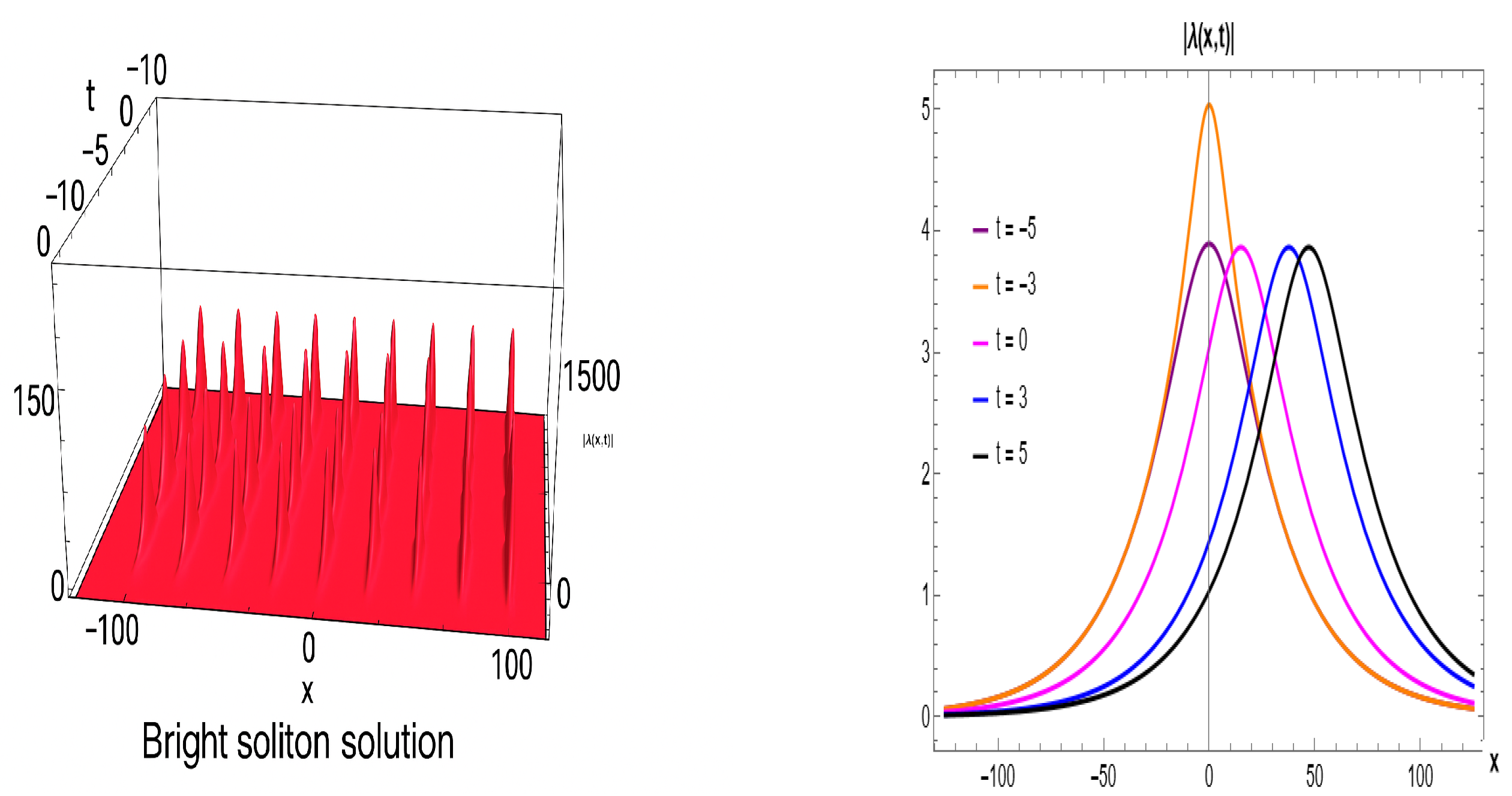
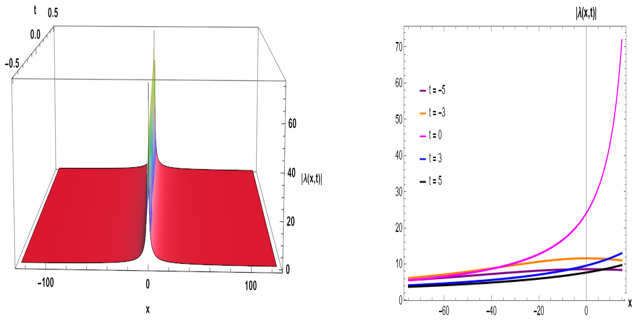
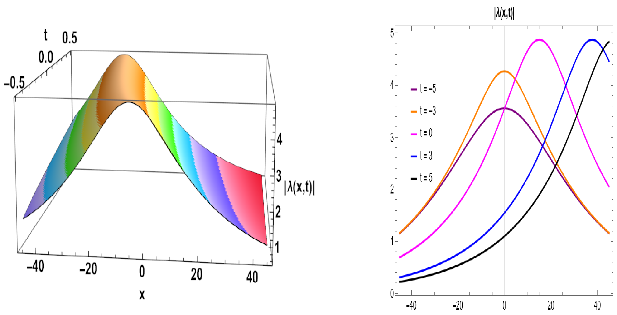
We obtained a variety of optical soliton solutions, including bright soliton (BS) solution represented by Figure 1 (Equation (25)), Figure 4 (Equation (33)), and Figure 10 (Equation (53)). A BS is a particular kind of solitary wave that travels through a medium without dispersing or changing form. This is a self-reinforcing wave phenomenon that is localized. Nonlinear wave equations, such as the NLSEs, are frequently used to mathematically characterize BS. The BS pulse in the context of the NLSE usually takes the form of a sech-shaped pulse. It may travel great distances while maintaining its form and amplitude because it is stable against disturbances. BSs do not disperse or spread out as they move, in contrast to most waves. When dispersion and nonlinearity combine in a range of physical systems, interesting phenomena known as band gaps (BSs) arise that shed light on the intricate dynamics of nonlinear wave propagation. 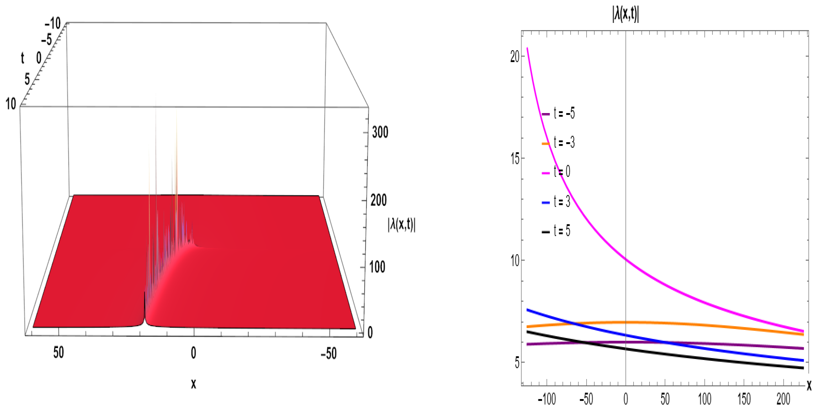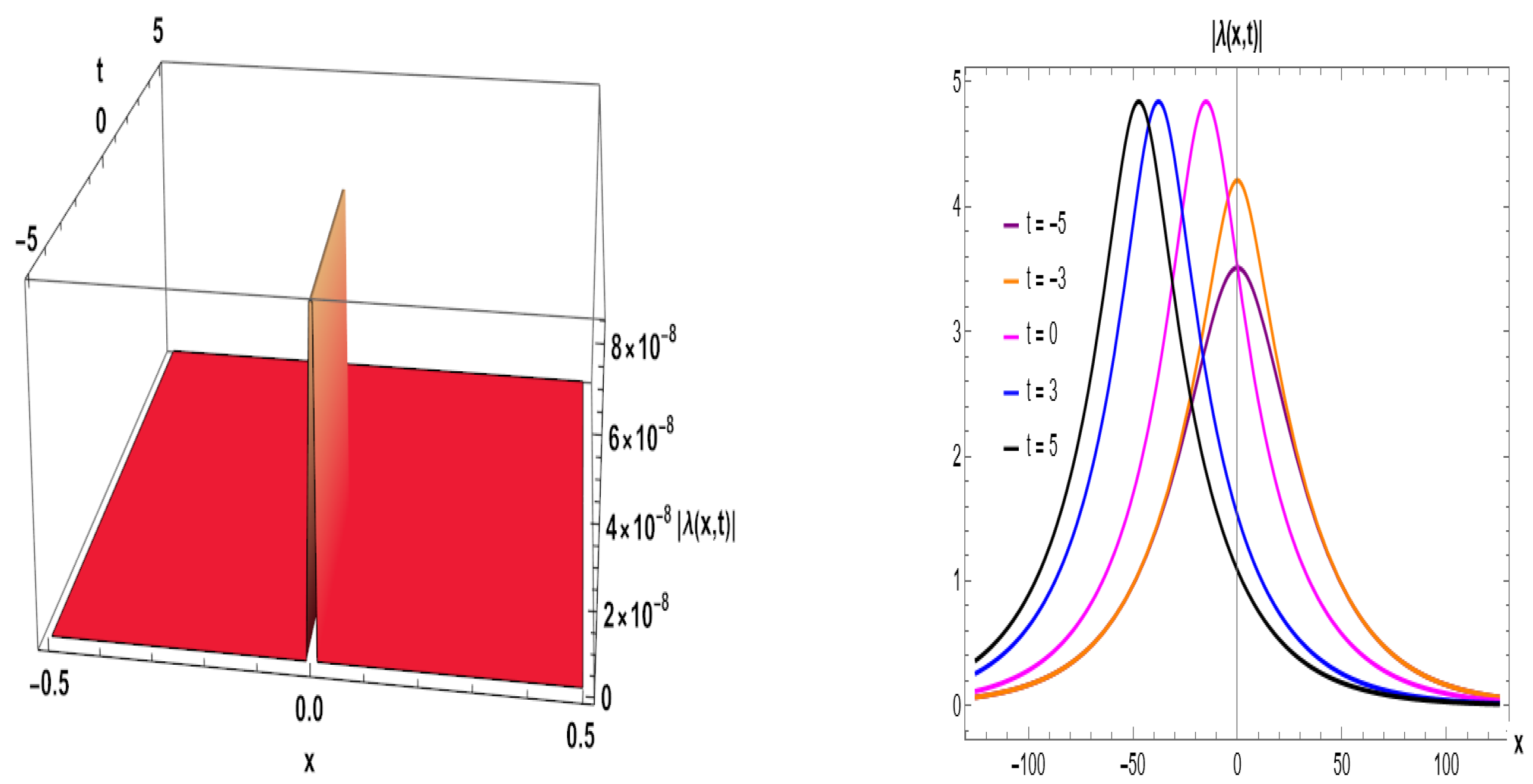Singular solutions (SSs) are represented in Figure 11 (Equation (54)). An SS solution is an example of a solitary wave solution to a particular family of nonlinear PDEs. Solitary waves are localized disturbances that travel through space without changing their direction or speed. A certain type of solitary wave called a soliton has the ability to maintain its shape even after colliding with other soliton. The term singular in single soliton solution frequently denotes the special and frequently noteworthy qualities that these solutions display. These solutions are helpful in a variety of domains, including nonlinear optics, fluid dynamics, and plasma physics, because of their capacity to hold their integrity and shape across extended distances.

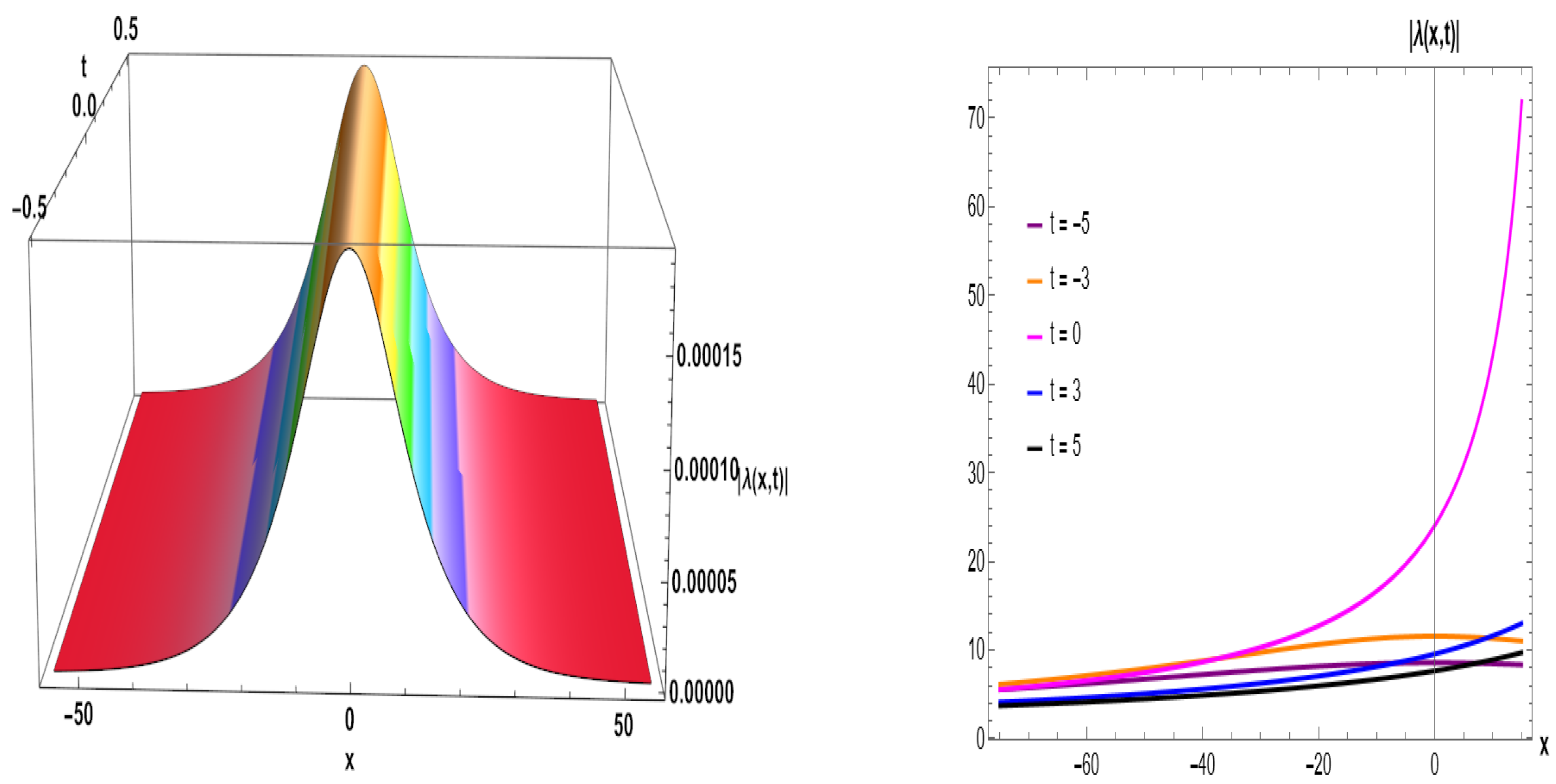
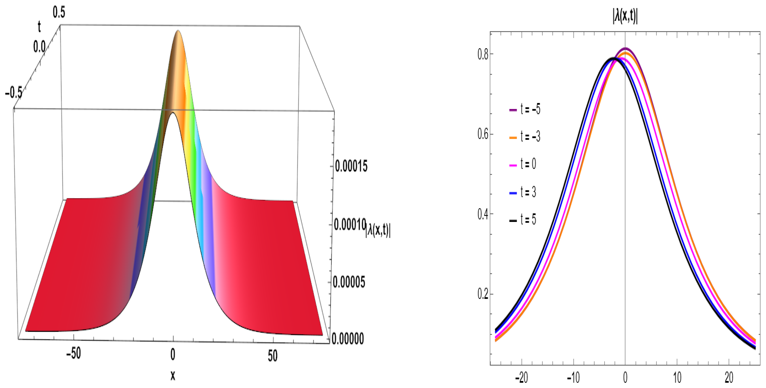
Periodic solutions represented in Figure 5 (Equation (34)), Figure 12 (Equation (60)), Figure 2 (Equation (26)), and Figure 13 (Equation (61)) occur when a function repeats its values at set intervals or periods. The fact that periodic functions repeat their values after predetermined periods is one of their essential characteristics. The largest value from the average value of a periodic function is known as its amplitude. It is possible to shift periodic functions along the x-axis without affecting their periodicity. A periodic function’s frequency in the context of trigonometric functions is correlated with its period and controls the oscillation rate. Periodic functions often arise as solutions to differential equations modeling phenomena with periodic behavior, such as oscillatory systems and wave propagation. We also encounter hyperbolic functions which are essential because they provide strong instruments for simulating and resolving a variety of issues including exponential growth, decay, and wave propagation.

A sort of soliton solution known as a Jacobian elliptic soliton (JES) solution is one that is produced using Jacobian elliptic functions (JEFs) which are unique functions that are employed to characterize periodic and doubly periodic solutions to nonlinear differential equations. JESs are represented in Figure 7 (Equation (41)) and Figure 8 (Equation (42)). For integrable systems such as the sine-Gordon equation or the Korteweg-de Vries equation, JEF is extremely helpful in determining solutions to solitary waves in the setting of soliton equations. Given the way the elliptic functions act properly, these solutions are regularly oscillatory or periodic in creation. A precise mathematical description of the wave’s behavior, including its shape, amplitude, speed, and periodicity, can usually be obtained using a JES solution by expressing the solitary wave solution in terms of JEF. The Weierstrass elliptic function (WEF) soliton describes the elliptic curves and are attributed to the German mathematician Weierstrass. WEFs are represented in Figure 9 (Equation (47)). WEFs can be used to extract equations such as the Korteweg-de Vries equation and NLSEs. WEFs represent periodic solutions. A WEF solution offers a mathematical framework for understanding the occurrence of solitary waves in terms of elliptic functions. This solution explains the wave’s shape, amplitude, speed, and periodicity, which is summarized in Table 3.

Table 3. Summary of Geometrical Structures and Solution Types.

Figure	Solution Type	Geometrical Characteristics	Physical Significance
Figure 1	Bright Soliton (Equation (25))	Bell-shaped pulse, symmetric and localized	Stable soliton structure, resists dispersion
Figure 2	Periodic Soliton (Equation (26))	Oscillatory waveform, modulated amplitude	Represents periodic nonlinear waves
Figure 3	Singular Soliton (Equation (27))	Sharp peak, fast decay, localized	Intense focusing; rogue wave-like structure
Figure 4	Bright Soliton (Equation (33))	Narrow symmetric peak	Weak localized waves; small amplitude soliton
Figure 5	Ultra-Narrow Soliton (Equation (34))	Sharp spike over flat base	High localization; ultra-compact solitons
Figure 6	Rational Soliton (Equation (35))	Growth toward singularity	Describes singular or blow-up behavior
Figure 7	Elliptic Soliton (Equation (41))	Symmetric smooth curve	Intermediate between periodic and solitary waves
Figure 8	Singular Soliton (Equation (42))	Steep peak with long tail	Energy burst or blow-up structure
Figure 9	Elliptic Complex Soliton (Equation (47))	Spike-rich surface; smooth envelope in 2D	Quasi-periodic soliton behavior
Figure 10	Bright Soliton (Equation (53))	Hill-shaped surface, symmetric curves	Sech-type soliton; robust structure
Figure 11	Bright Soliton (Equation (54))	Sharp symmetric peak; dome-like shape	Stable propagation with coherent wave
Figure 12	Decaying Soliton (Equation (60))	Plateau surface; decreasing amplitude	Soliton dissipation over time
Figure 13	Rational Decaying Soliton (Equation (61))	Low amplitude hill, exponential decay	Non-conservative wave energy behavior

Table 3. Summary of Geometrical Structures and Solution Types.

Figure	Solution Type	Geometrical Characteristics	Physical Significance
Figure 1	Bright Soliton (Equation (25))	Bell-shaped pulse, symmetric and localized	Stable soliton structure, resists dispersion
Figure 2	Periodic Soliton (Equation (26))	Oscillatory waveform, modulated amplitude	Represents periodic nonlinear waves
Figure 3	Singular Soliton (Equation (27))	Sharp peak, fast decay, localized	Intense focusing; rogue wave-like structure
Figure 4	Bright Soliton (Equation (33))	Narrow symmetric peak	Weak localized waves; small amplitude soliton
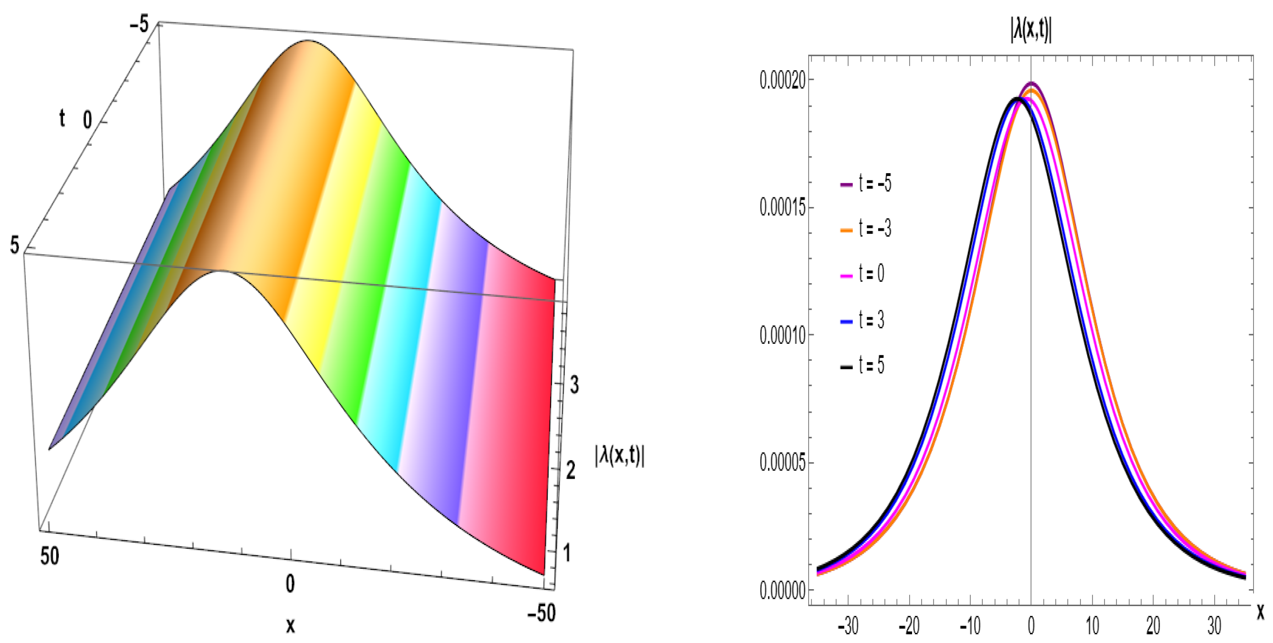
Figure 5	Ultra-Narrow Soliton (Equation (34))	Sharp spike over flat base	High localization; ultra-compact solitons
Figure 6	Rational Soliton (Equation (35))	Growth toward singularity	Describes singular or blow-up behavior
Figure 7	Elliptic Soliton (Equation (41))	Symmetric smooth curve	Intermediate between periodic and solitary waves
Figure 8	Singular Soliton (Equation (42))	Steep peak with long tail	Energy burst or blow-up structure
Figure 9	Elliptic Complex Soliton (Equation (47))	Spike-rich surface; smooth envelope in 2D	Quasi-periodic soliton behavior
Figure 10	Bright Soliton (Equation (53))	Hill-shaped surface, symmetric curves	Sech-type soliton; robust structure
Figure 11	Bright Soliton (Equation (54))	Sharp symmetric peak; dome-like shape	Stable propagation with coherent wave
Figure 12	Decaying Soliton (Equation (60))	Plateau surface; decreasing amplitude	Soliton dissipation over time
Figure 13	Rational Decaying Soliton (Equation (61))	Low amplitude hill, exponential decay	Non-conservative wave energy behavior

Figure 1. Bright soliton for Equation (25) for given parameters ($\mathfrak{r}=0.25$, $\mho =0.5$, $ϵ=5$, $\psi =-5$, $\Theta =2$, $\epsilon =10$, $\delta =-12$, $I=2$). (left) 3D visual. (right) 2D graph.

Figure 1. Bright soliton for Equation (25) for given parameters ($\mathfrak{r}=0.25$, $\mho =0.5$, $ϵ=5$, $\psi =-5$, $\Theta =2$, $\epsilon =10$, $\delta =-12$, $I=2$). (left) 3D visual. (right) 2D graph.

Figure 2. Periodic shape profile of Equation (26) for given parameters ($\mathfrak{r}=0.25$, $\mho =0.5$, $ϵ=-5$, $\psi =5$, $\Theta =-8$, $\epsilon =-15$, $\delta =2$, $I=-2$). (left) 3D depiction. (right) 2D graph.

Figure 2. Periodic shape profile of Equation (26) for given parameters ($\mathfrak{r}=0.25$, $\mho =0.5$, $ϵ=-5$, $\psi =5$, $\Theta =-8$, $\epsilon =-15$, $\delta =2$, $I=-2$). (left) 3D depiction. (right) 2D graph.

Figure 3. Rational dynamical behavior of Equation (27) for given parameters ($\mathfrak{r}=0.15$, $\mho =0.5$, $ϵ=-5$, $\psi =5$, $\Theta =5$, $\epsilon =1$, $\delta =5$, $I=-1$). (left) 3D plot. (right) 2D representation.

Figure 3. Rational dynamical behavior of Equation (27) for given parameters ($\mathfrak{r}=0.15$, $\mho =0.5$, $ϵ=-5$, $\psi =5$, $\Theta =5$, $\epsilon =1$, $\delta =5$, $I=-1$). (left) 3D plot. (right) 2D representation.

Figure 4. Bell shaped plot of Equation (33) for given parameters ($\mathfrak{r}=0.25$, $\mho =0.5$, $\epsilon =-5$, $\psi =5$, $\Theta =25$, $\xi =-0.5$, $\delta =5$, $I=2$, $O=3$). (left) 3D plot. (right) 2D visual.

Figure 4. Bell shaped plot of Equation (33) for given parameters ($\mathfrak{r}=0.25$, $\mho =0.5$, $\epsilon =-5$, $\psi =5$, $\Theta =25$, $\xi =-0.5$, $\delta =5$, $I=2$, $O=3$). (left) 3D plot. (right) 2D visual.

Figure 5. Ultra-narrow soliton: The 3D and 2D graphs of Equation (34) for given parameters ($\mathfrak{r}=0.25$, $\mho =0.5$, $ϵ=-5$, $\psi =5$, $\Theta =25$, $\epsilon =-0.5$, $\delta =5$, $I=2$, $O=3$). (left) 3D graph. (right) 2D representation.

Figure 5. Ultra-narrow soliton: The 3D and 2D graphs of Equation (34) for given parameters ($\mathfrak{r}=0.25$, $\mho =0.5$, $ϵ=-5$, $\psi =5$, $\Theta =25$, $\epsilon =-0.5$, $\delta =5$, $I=2$, $O=3$). (left) 3D graph. (right) 2D representation.

Figure 6. Rational soliton representation of Equation (35) for given parameters ($\mathfrak{r}=0.25$, $\mho =0.5$, $ϵ=-5$, $\psi =5$, $\Theta =125$, $\epsilon =-0.75$, $\delta =55$, $O=3$). (left) 3D plot. (right) 2D diagram.

Figure 6. Rational soliton representation of Equation (35) for given parameters ($\mathfrak{r}=0.25$, $\mho =0.5$, $ϵ=-5$, $\psi =5$, $\Theta =125$, $\epsilon =-0.75$, $\delta =55$, $O=3$). (left) 3D plot. (right) 2D diagram.

Figure 7. Elliptic soliton for Equation (41) for given parameters ($\mathfrak{r}=5.25$, $\mho =0.5$, $ϵ=5$, $\psi =5$, $\Theta =-2.9$, $\epsilon =53$, $\delta =5$, $I=3$, $\mathfrak{m}=1$). (left) 3D representation. (right) 2D diagram.

Figure 7. Elliptic soliton for Equation (41) for given parameters ($\mathfrak{r}=5.25$, $\mho =0.5$, $ϵ=5$, $\psi =5$, $\Theta =-2.9$, $\epsilon =53$, $\delta =5$, $I=3$, $\mathfrak{m}=1$). (left) 3D representation. (right) 2D diagram.

Figure 8. Singular like profile of Equation (42) for given parameters ($\mathfrak{r}=5.25$, $\mho =0.5$, $ϵ=5$, $\psi =5$, $\Theta =9$, $\epsilon =3$, $\delta =5$, $I=3$, $\mathfrak{m}=1$). (left) 3D plot. (right) 2D graph.

Figure 8. Singular like profile of Equation (42) for given parameters ($\mathfrak{r}=5.25$, $\mho =0.5$, $ϵ=5$, $\psi =5$, $\Theta =9$, $\epsilon =3$, $\delta =5$, $I=3$, $\mathfrak{m}=1$). (left) 3D plot. (right) 2D graph.

Figure 9. Elliptic complex soliton for Equation (47) for given parameters ($\mathfrak{r}=0.25$, $\mho =0.5$, $ϵ=12$, $\psi =5$, $\Theta =2$, $\epsilon =1$, $\delta =5$). (left) 3D plot. (right) 2D diagram.

Figure 9. Elliptic complex soliton for Equation (47) for given parameters ($\mathfrak{r}=0.25$, $\mho =0.5$, $ϵ=12$, $\psi =5$, $\Theta =2$, $\epsilon =1$, $\delta =5$). (left) 3D plot. (right) 2D diagram.

Figure 10. Bright type plot of Equation (53) for given parameters ($\mathfrak{r}=0.25$, $\mho =0.5$, $ϵ=5$, $\psi =5$, $\Theta =2$, $\epsilon =-10$, $\delta =5$, $I=2$, $O=3$). (left) 3D plot. (right) 2D visual.

Figure 10. Bright type plot of Equation (53) for given parameters ($\mathfrak{r}=0.25$, $\mho =0.5$, $ϵ=5$, $\psi =5$, $\Theta =2$, $\epsilon =-10$, $\delta =5$, $I=2$, $O=3$). (left) 3D plot. (right) 2D visual.

Figure 11. Bell type with sharp symmetric peak shape profile of Equation (54) for given parameters ($\mathfrak{r}=0.25$, $\mho =0.5$, $ϵ=5$, $\psi =5$, $\Theta =2$, $\epsilon =-10$, $\delta =5$, $I=2$, $O=3$). (left) 3D graph. (right) 2D diagram.

Figure 11. Bell type with sharp symmetric peak shape profile of Equation (54) for given parameters ($\mathfrak{r}=0.25$, $\mho =0.5$, $ϵ=5$, $\psi =5$, $\Theta =2$, $\epsilon =-10$, $\delta =5$, $I=2$, $O=3$). (left) 3D graph. (right) 2D diagram.

Figure 12. The decaying soliton dynamical behavior of Equation (60) for given parameters ($\mathfrak{r}=0.25$, $\mho =0.5$, $ϵ=5$, $\psi =5$, $\Theta =2$, $\epsilon =-10$, $\delta =-5$, $I=-2$, $O=3$). (left) 3D plot. (right) 2D graph.

Figure 12. The decaying soliton dynamical behavior of Equation (60) for given parameters ($\mathfrak{r}=0.25$, $\mho =0.5$, $ϵ=5$, $\psi =5$, $\Theta =2$, $\epsilon =-10$, $\delta =-5$, $I=-2$, $O=3$). (left) 3D plot. (right) 2D graph.

Figure 13. Rational decaying soliton of Equation (61) for given parameters ($\mathfrak{r}=0.25$, $\mho =0.5$, $\epsilon =5$, $\psi =5$, $\Theta =2$, $\xi =-10$, $\delta =-5$, $I=2$, $O=3$). (left) 3D visual (right) 2D diagram.

Figure 13. Rational decaying soliton of Equation (61) for given parameters ($\mathfrak{r}=0.25$, $\mho =0.5$, $\epsilon =5$, $\psi =5$, $\Theta =2$, $\xi =-10$, $\delta =-5$, $I=2$, $O=3$). (left) 3D visual (right) 2D diagram.

5. Novelty of Our Work

The present study introduces a novel and comprehensive analytical framework to explore the diverse family of optical soliton solutions for the TFCQ-NLSE by employing the sub-ODE method coupled with the beta-fractional derivative. Unlike existing studies which focus primarily on classical solution techniques or omit fractional dynamics, our approach yields a significantly broader and richer set of solutions, including bright, singular, periodic, rational, Jacobian elliptic, Weierstrass elliptic, and hyperbolic solitons. The methodology captures both localized and oscillatory behaviors and incorporates fractional memory effects, which are crucial for modeling realistic physical systems with hereditary properties. Notably, the use of advanced ansatz functions in symbolic computation enables the derivation of multi-wave structures and interaction profiles. The inclusion of both geometric interpretation and physical significance, as systematically presented in Table 2, provides a clear classification of solution dynamics. Furthermore, the comparative analysis in Table 1 demonstrates that this is the first attempt to simultaneously implement the sub-ODE method and fractional derivatives for the TFCQ-NLSE. The model’s generality and flexibility are substantiated through 2D and 3D visualizations, revealing the stability, decay, blow-up, and periodic nature of solutions under varying physical parameters. Overall, this work fills a substantial research gap and offers a unified analytical structure for understanding complex nonlinear wave dynamics in optical and physical systems.

6. Conclusions

In this study, a new analytical framework is introduced for solving the TFCQ-NLSE by employing the sub-ODE method in conjunction with the recently proposed beta fractional derivative, which more accurately captures memory effects compared to classical formulations. A diverse spectrum of explicit optical soliton solutions is derived, including bright (bell-shaped), periodic, rational, Jacobian elliptic, Weierstrass elliptic, singular, and hyperbolic waveforms. The solutions are examined both analytically and graphically, highlighting distinct geometric features such as solitary peaks, decaying tails, oscillatory patterns, and singular spikes, thereby enhancing the physical understanding of nonlinear wave dynamics. These geometries are well-represented in 2D and 3D plots under various parameter sets, revealing the sensitivity of wave behavior to the interplay of dispersion and cubic–quintic nonlinearities. The adaptive nature of the model enables its applicability to a wide range of complex real-world phenomena, including optical signal processing, fiber optics, quantum systems, and laser–tissue interactions. The novelty of this work lies in the application of the sub-ODE technique to a fractional framework, leading to a unified and systematic generation of new soliton families, many of which have not been reported previously in the literature, thereby contributing significantly to the analytical understanding of nonlinear pulse propagation in optical and quantum media.

Although this study successfully presents a wide range of analytical soliton solutions to the TFCQ-NLSE using the sub-ODE method and beta-fractional derivative, it is primarily limited to specific parametric forms and idealized conditions. While the sub-ODE method proves highly effective in generating diverse exact solutions including bright, singular, rational, periodic, and elliptic solitons, it inherently depends on selecting appropriate auxiliary equations and trial function forms. This reliance can restrict its applicability in more generalized or complex scenarios, particularly when dealing with perturbations, variable coefficients, damping effects, or arbitrary boundary conditions, which are often present in realistic optical systems. Additionally, the current analysis is confined to one-dimensional wave propagation and does not capture multidimensional or multi-soliton interaction phenomena. The method also does not inherently account for the stability or dynamic evolution of the obtained solutions under external influences. In future work, we aim to extend this study by incorporating stability and modulation instability analysis, higher-order dispersion effects, and advanced numerical or machine learning-based approaches such as physics informed neural networks (PINNs). Moreover, generalizing the methodology to coupled systems and validating results through simulations or experimental setups will further enhance the scope, applicability, and physical relevance of the proposed model.

7. Nomenclature and Physical Interpretations

• $\chi (x,t)$ is the function on which the ℧-fractional derivative is applied.
• ℧ is the order of fractional differentiation such that $0<\mho \le 1$.
• $h=\vartheta {\left(t+{\displaystyle \frac{1}{\Gamma \left(\mathcal{V}\right)}}\right)}^{\mho -1}$ is a small real quantity used in the $\mathcal{V}$-derivative formulation.
• $\Gamma$ is the Gamma function.
• $\lambda (x,t)$ is the complex wave function that represents the light pulse’s phase and amplitude.
• $i=\sqrt{-1}$ denotes the imaginary unit.
• $ϵ$ denotes the coefficient for group velocity dispersion (GVD).
• $\delta$ indicates the contribution from the time-fractional derivative term.
• $Y\left(\right|\lambda \left|\right)=\left(O\right|\lambda |+{I\left|\lambda \right|}^2)$ represents the nonlinearity contribution, where O and I are model constants.
• ${\left|\lambda \right|}^2$ denotes the optical intensity of the wave function.
• $\Lambda \left(v\right)$ is the amplitude part of the complex wave function after transformation.
• $\varrho (x,t)$ denotes the phase of the wave function.
• $v={\displaystyle \frac{x-\epsilon {\left(t+{\displaystyle \frac{1}{\Gamma (\mho )}}\right)}^{\mho }}{\mho }}$ is the transformed spatial variable.
• $\varrho (x,t)={\nu }_{1}x-{\displaystyle \frac{t{\left(t+{\displaystyle \frac{1}{\Gamma (\mho )}}\right)}^{\mho }}{\mho }}$ is the transformed phase function.
• $\psi >0$ is a constant used in the solution ansatz.
• $\kappa \left(v\right)$ is an auxiliary function satisfying the sub-ODE.
• $\Xi$ is a scaling parameter in the solution ansatz.
• $\Theta$ is the power parameter appearing in the homogeneous balancing.
• $\mathcal{A},\mathcal{B},\mathcal{C},\mathcal{D},\mathcal{F}$ are arbitrary constants used in the sub-ODE.

References

- Arnous, A.H.; Mirzazadeh, M. Application of the generalized Kudryashov method to the Eckhaus equation. Nonlinear Anal. Model. Control. 2016, 21, 577–586. [Google Scholar] [CrossRef]
- Mirzazadeh, M.; Eslami, M.; Arnous, A.H. Dark optical solitons of Biswas-Milovic equation with dual-power law nonlinearity. Eur. Phys. J. 2015, 4, 130. [Google Scholar] [CrossRef]
- Arnous, A.H.; Moraru, L. Optical solitons with the complex Ginzburg-Landau equation with Kudryashov’s law of refractive index. Mathematics 2022, 10, 3456. [Google Scholar] [CrossRef]
- Arnous, A.H.H. Optical solitons with Biswas-Milovic equation in magneto-optic waveguide having Kudryashov’s law of refractive index. Optik 2021, 247, 167987. [Google Scholar] [CrossRef]
- Rizvi, S.T.R.; Seadawy, A.R.; Raza, U. Some advanced chirped pulses for generalized mixed for nonlinear Schrödinger dynamical equation. Chaos Solitons Fractals 2022, 163, 112575. [Google Scholar] [CrossRef]
- Seadawy, A.R.; Rizvi, S.T.R.; Ahmed, S. Weierstrass and Jacobi elliptic, bell and kink type, lumps, Ma and Kuznetsov breathers with rogue wave solutions to the dissipative nonlinear Schrödinger equation. Chaos Solitons Fractals 2022, 150, 112258. [Google Scholar] [CrossRef]
- Aziz, N.; Seadawy, A.R.; Ali, K.; Sohail, M.; Rizvi, S.T.R. The nonlinear Schrödinger equation with polynomial law nonlinearity: Localized chirped optical and solitary wave solutions. Opt. Quantum Electron. 2022, 54, 458. [Google Scholar] [CrossRef]
- Ali, I.; Rizvi, S.T.R.; Abbas, S.O.; Zhou, Q. Optical solitons for modulated compressional dispersive Alfven and Heisenberg ferromagnetic spin chains. Res. Phy. 2019, 15, 102714. [Google Scholar] [CrossRef]
- Rezazadeh, H. New solitons solutions of the complex Ginzburg-Landau equation with Kerr law nonlinearity. Optik 2018, 167, 218–227. [Google Scholar] [CrossRef]
- Akinyemi, L.; Mirzazadeh, M.; Hosseini, K. Solitons and other solutions of perturbed nonlinear Biswas-Milovic equation with Kudryashov’s law of refractive index. Nonlinear Anal. Model. Control. 2022, 27, 1–17. [Google Scholar] [CrossRef]
- Rizvi, S.T.R.; Abbas, S.O.; Ali, K. Optical solitons for non-Kerr law nonlinear Schrödinger equation with third and fourth order dispersions. Chin. J. Phys. 2019, 60, 133–140. [Google Scholar] [CrossRef]
- Zhang, C.; Zhang, Z. Application of the enhanced modified simple equation method for Burger-Fisher and modified Volterra equations. Adv. Differ. Equ. 2017, 2017, 145. [Google Scholar] [CrossRef]
- Mathanaranjan, T.; Rezazadeh, H.; Senol, M.; Akinyemi, L. Optical singular and dark solitons to the non-linear Schrödinger equation in magneto-optic waveguides with anti-cubic nonlinearity. Opt. Quant. Electron. 2021, 53, 722. [Google Scholar] [CrossRef]
- Rabie, W.B.; Ahmed, H.M. Cubic-quartic optical soliton and other solutions for twin-core couplers with polynomial lawof nonlinearity using the extended F-expansion method. Optik 2023, 55, 637. [Google Scholar]
- Rafiq, M.H.; Jannat, N.; Rafiq, M.N. Sensitivity analysis and analytical study of the three-component coupled NLS-type equations in fiber optics. Opt. Quant. Electron. 2023, 55, 637. [Google Scholar] [CrossRef]
- Faridi, A.W.; Asjad, I.M.; Jhangeer, A.; Yusuf, A.; Sulaiman, T.A. The weakly non-linear waves propagation for Kelvin-Helmhotz instability in the mangnetohydrodynamic flow impelled by fractional theory. Optik 2023, 55, 172. [Google Scholar]
- Mathanaranjan, T. New Jacobi elliptic solutions and other solutions in optical metamaterials having higher-order dispersion and its stability analysis. Int. J. Appl. Comput. Math. 2023, 9, 66. [Google Scholar] [CrossRef]
- Liang, S.; Jeffrey, D.J. Comparison of homotopy analysis method and homotopy perturbation method through an evolution equation. Commun. Non-linear Sci. Numer. Simul. 2009, 14, 4057–4064. [Google Scholar] [CrossRef]
- Mohanty, S.K.; Kravchenko, O.V.; Deka, M.K.; Dev, A.N.; Churika, D.V. The exact soltion of the (2 + 1)-dimension Kadomtsev-Petviashvili equation with variable coefficient by extended generalized (G’/G)-expansion method. J. King Saud. Univ. Sci. 2023, 35, 102358. [Google Scholar] [CrossRef]
- Faridi, A.W.; Bakar, M.A.; Akgul, A.; El-Rehman, M.A.; Din, M.S.E. Exact fractional soliton solutions of thin-film ferroelectric material equation by analytic approaches. Alex. Eng. J. 2023, 78, 483–497. [Google Scholar] [CrossRef]
- Akbar, M.A.; Abdullah, F.A.; Islam, M.T.; Sharif, M.A.A.; Osman, M.S. New solutions of the soliton type of shallow water waves and superconductivity models. Res. Phys. 2023, 44, 106180. [Google Scholar] [CrossRef]
- Khater, M.M.A.; Ghanbari, B. On the solitary wave solutions and physical characterization of gas diffusion in a homogeneous medium via some efficient techniques. Eur. Phys. J. Plus. 2021, 136, 447. [Google Scholar] [CrossRef]
- Al-Mamun, A.; Ananna, S.N.; An, T.; Asaduzzaman, M.; Miah, M.M. Solitary wave structures of a family of 3D fractional WBBM equation via the tanh-coth approach. Partial. Differ. Equ. Appl. Math. 2022, 5, 100237. [Google Scholar] [CrossRef]
- Khatun, M.M.; Akbar, M.A. New optical soliton solutions to the space-time fractional perturbed Chen-Lee-Liu equation. Res. Phys. 2023, 46, 106306. [Google Scholar] [CrossRef]
- Khalil, R.; Horani, M.A.; Yousef, A.; Sababheh, M. A new definition of fractional derivative. J. Comput. Appl. Math. Comput. Appl. Math. 2014, 264, 65–70. [Google Scholar] [CrossRef]
- Mathanaranjan, T. An effective technique for the conformable space-time fractional cubic-quartic nonlinear Schrödinger equation with different laws of nonlinearity. Comput. Methods Differ. Equ. 2022, 10, 701–715. [Google Scholar]
- Mathanaranjan, T.; Vijayakumar, D. New soliton solutions in Nano-Fibers with space-time fractional derivatives. Fractals 2022, 30, 1–10. [Google Scholar] [CrossRef]
- Akbar, M.A.; Abdullah, F.A.; Khatun, M.M. An invetsigation of optical solitons of the fractional cubic-quintic nonlinear pulse propagation model: An analytic approach and the impact of fractional derivative. Opt. Quantum Electron. 2024, 56, 58. [Google Scholar] [CrossRef]
- Tariq, K.U.; Khater, M.M.A.; Inc, M. On some novel bright, dark and optical solitons to the cubic-quintic nonlinear non-paraxial pulse propagation model. Opt. Quant. Electron. 2021, 53, 726. [Google Scholar] [CrossRef]
- Rizvi, S.T.R.; Seadawy, A.R.; Raza, U. Detailed analysis for chirped pulses to cubic-quintic nonlinear nonparaxial pulse propagation model. J. Geom. Phys. 2022, 178, 104561. [Google Scholar] [CrossRef]
- Jlali, L.; Rizvi, S.T.; Shabbir, S.; Seadawy, A.R. Study of Optical Solitons and Quasi-Periodic Behaviour for the Fractional Cubic Quintic Nonlinear Pulse Propagation Model. Mathematics 2025, 13, 2117. [Google Scholar] [CrossRef]
- Zhong, X.; Du, X.; Cheng, K. Evolution of finite energy Airy pulses and soliton generation in optical fibers with cubic-quintic nonlinearity. Opt. Express 2015, 23, 29467–29475. [Google Scholar] [CrossRef]
- Ahmed, S.; Hashem, A.F.; Rizvi, S.T.R.; Seadawy, A.R. Characterizing the physical and dynamical properties of lump, rogue waves and their interactions for a cascaded system with spatio-temporal dispersion and Kerr nonlinearity. AIMS Math. 2025, 10, 16498–16525. [Google Scholar] [CrossRef]
- Zayed, E.M.E.; Alngara, E.M.M.; Biswasb, A.; Trikif, H.; Yıldırımg, Y.; Alshomranic, A.S. Chirped and chirp-free optical solitons in fiber Bragg gratings with dispersive reflectivity having quadratic-cubic nonlinearity by sub-ODE approach. Optik 2020, 203, 163993. [Google Scholar] [CrossRef]