Analytical and Numerical Treatment of Evolutionary Time-Fractional Partial Integro-Differential Equations with Singular Memory Kernels

Abstract

Evolution equations with fractional-time derivatives and singular memory kernels are used for modeling phenomena exhibiting hereditary properties, as they effectively incorporate memory effects into their formulation. Time-fractional partial integro-differential equations (FPIDEs) represent a significant class of such evolution equations and are widely used in diverse scientific and engineering fields. In this study, we use the $\mathrm{sinc}$-collocation and iterative Laplace transform methods to solve a specific FPIDE with a weakly singular kernel. Specifically, the $\mathrm{sinc}$-collocation method is applied to discretize the spatial domain, while a combination of numerical techniques is utilized for temporal discretization. Then, we prove the convergence analytically. To compare the two methods, we provide two examples. We notice that both the $\mathrm{sinc}$-collocation and iterative Laplace transform methods provide good approximations. Moreover, we find that the accuracy of the methods is influenced by fractional order $\alpha \in (0,1)$ and the memory-kernel parameter $\beta \in (0,1)$. We observe that the error decreases as $\beta$ increases, where the kernel becomes milder, which extends the single-value study of $\beta =1/2$ in the literature.

1. Introduction

While classical integer-order derivatives remain highly effective for modeling many phenomena, their locality operators may not fully capture certain complex phenomena in applied mathematics that depend on a system’s past states, particularly those with non-local characteristics. Fractional (non-local) derivatives can offer an alternative to the classical framework by offering additional flexibility for describing processes with memory and hereditary effects, including those in epidemiology [1,2], viscoelastic materials [3], and gas-film dynamics [4]. Nevertheless, it is challenging to solve most fractional differential equations analytically. This situation has led to the development of numerous numerical techniques for solving fractional differential equations. Numerous studies have been conducted on integro-differential equations. The topic of applying various methods to solve integral equations with fractional derivatives has been the subject of multiple prior studies. For instance, fractional integro-differential equations of weakly singular kernels have been solved using the $\mathrm{sinc}$-collocation method [5], Galerkin spectral and finite difference methods [6], the mesh-free methods [7,8], the Haar wavelet method [9], double Laplace transform [10], parallel-in-time (PinT) algorithm [11,12], and high-order finite difference [13]. Moreover, a $\mathrm{sinc}$-Galerkin approach to solving the fourth-order partial integro-differential equation with a weakly singular kernel is proposed in [14].

In this work, we examine the $\mathrm{sinc}$-collocation and the iterative Laplace methods to solve a time-fractional partial integro-differential equation (FPIDE) with a weakly singular kernel. Let $u(x,t)$ be a differentiable function. Then, the Caputo-fractional derivative of order $\alpha \in (0,1)$ is defined as follows [15]:

$$D_t^{\alpha }u(x,t)=J_t^{1-\alpha }{\displaystyle \frac{\partial u(x,t)}{\partial t}}={\displaystyle \frac{1}{\Gamma (1-\alpha )}}{\int }_0^t{\displaystyle \frac{1}{{(t-\eta )}^{\alpha }}}{\displaystyle \frac{\partial u(r,\eta )}{\partial \eta }}d\eta .$$

(1)

where $J_t^{\alpha }$ is the Riemann–Liouville fractional integral operator is given by the following:

$$J_t^{\alpha }u(x,t)={\displaystyle \frac{1}{\Gamma \left(\alpha \right)}}{\int }_0^t{\displaystyle \frac{1}{{(t-\eta )}^{1-\alpha }}}u(x,\eta )d\eta ,\alpha >0.$$

We adopt the Caputo definition of the fractional derivative here because it is well-suited to modeling physical processes with classical initial conditions.

Consider FPIDE with a weakly singular kernel:

$$\begin{array}{cc}\hfill & D_t^{\alpha }u(x,t)=u_{xx}(x,t)+{\int }_0^t{(t-s)}^{\beta -1}{u}_{xx}(x,s)ds+H(x,t),(x,t)\in \Omega \hfill \\ \hfill & \mathrm{Boundary}\mathrm{conditions}:u(a,t)=u(b,t)=0,\hfill \\ \hfill & \mathrm{Initial}\mathrm{condition}:u(x,0)=g\left(x\right),\hfill \end{array}$$

(2)

where $\alpha ,\beta \in (0,1)$, $D^{\alpha }$ is the Caputo-fractional derivative, $\Omega =[a,b]\times [0,T]$, and $H(x,t)$ is a given function.

To guarantee the existence of a unique solution of Equation (2) in $C([0,T],L^2(a,b))$, we assume that $g\left(x\right)\in L^2(a,b)$, the source term $H(x,t)\in L^2(\Omega )$, and the kernel ${(t-s)}^{\beta -1}$ is completely monotone. A comprehensive review of the relevant frameworks and detailed proofs can be found in [16]. In the rest of the manuscript, we assume that the solution $u(x,t)$ of (2) is unique and sufficiently smooth in both time and space, to consider the second-order weighted and shifted Grünwald difference formula to discretize the Caputo derivative in Equation (2), see, e.g., [17].

The parameter $\beta \in (0,1)$ is called the order of the memory kernel, and it represents the order of singularity in the kernel ${(t-s)}^{\beta -1}$ when $s=t$. This kind of singularity leads to a convergent integral; hence, Equation (2) is said to have a weakly singular kernel. In this work, we aim to solve Equation (2) and discuss the influence of the orders of the fractional derivative $\alpha$ and memory kernel $\beta$ on the robustness of the proposed methods. This kernel models a secondary relaxation mechanism that decays, allowing Equation (2) to capture both instantaneous and retarded diffusion. Applications include anomalous tracer transport in fractured media [18], thermal waves in polymers [19], and charge migration in amorphous semiconductors [20]. Recent analytical and numerical works study related initial–boundary value problems [21,22], underscoring the current interest in mixed Caputo–Volterra models. In [5], the authors studied the solution of Equation (2) when $\beta =0.5$. However, varying $\beta$ in $(0,1)$ will allow testing the accuracy of our proposed methods across a range of kernel singularities as the kernel becomes sharper when $\beta \to 0$ or milder when $\beta \to 1$ [23].

The paper is organized as follows: Section 2 presents the spatial discretization of $u_{xx}$ in Equation (2) using the $\mathrm{sinc}$-collocation method, along with related convergence results. In Section 3, the time-fractional derivative and integral term in Equation (2) are approximated using the weighted and shifted Grünwald operator and a quadrature formula based on the product trapezoidal integration rule, respectively. Section 4 establishes the convergence results of the proposed method. An overview of the iterative Laplace transform method is provided in Section 5. Section 6 presents two numerical examples that illustrate the implementation of the proposed method and its comparison with the iterative Laplace transform method. Finally, Section 7 discusses the obtained results.

2. The $\mathbf{sinc}$-Collocation Method for Spatial Discretization

In this section, we provide notations and definitions and review the main results for the $\mathrm{sinc}$-collocation method [24,25]. Throughout this manuscript, we denote the set of all integers, the real line, and the complex plane by $\mathbb{Z}$, $\mathbb{R}$, and $\mathbb{C}$, respectively.

First, we begin by defining the $\mathrm{sinc}$ function, which is a function defined on the entire set of real numbers $\mathbb{R}$ by

$$\mathrm{sinc}\left(x\right)=\left\{\begin{array}{cc}{\displaystyle \frac{sin\left(\pi x\right)}{\pi x}},\hfill & x\ne 0,\hfill \\ 1,\hfill & x=0.\hfill \end{array}\right.$$

For the $\mathrm{sinc}$-collocation method, we derive its basis from the Whittaker cardinal functions

$$\mathcal{S}(j,h_x)\left(x\right)=\mathrm{sinc}\left({\displaystyle \frac{x-j{h}_x}{h_x}}\right)$$

for $j\in \mathbb{Z}$ and any step size $h_x>0$. Note that the function $\mathcal{S}(j,h_x)\left(x\right)$ is a shifted and scaled version of the function $\mathrm{sinc}\left(x\right)$, that is, it is symmetric about $x=j{h}_x$. More precisely, the parameter j introduces a horizontal shift, moving the center of symmetry of $\mathrm{sinc}\left(x\right)$ from $x=0$ to $x=j{h}_x$, while $h_x$ scales the function accordingly, see Figure 1.

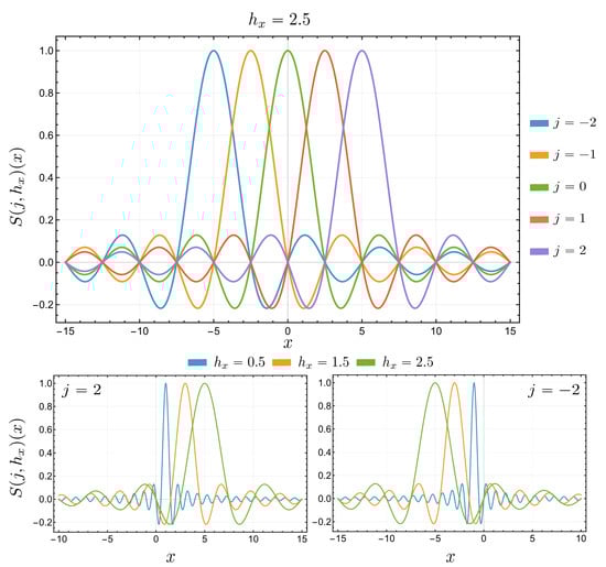
Figure 1. The symmetry of the function $\mathcal{S}(j,h_x)\left(x\right)$ around $x=j{h}_x$ with Row 1: $j=0,\pm 1,\pm 2$ when $h_x=2.5$, Row 2: $h_x=0.5,1.5,2.5$ when $j=\pm 2$. The parameter j determines the horizontal shift, and $h_x$ controls the scaling.

Consequently, for any function $f:\mathbb{R}\to \mathbb{R}$, we define the series

$$\mathcal{C}(f,h_x)\left(x\right)=\sum _{j=-\infty }^{\infty }f\left(jh\right)\mathcal{S}(j,h_x)\left(x\right)$$

as the Whittaker cardinal expansion of f, provided it converges [26]. Fix $0<d\le \frac{\pi }{2}$. For this fixed d, we choose the infinite strip-shaped region ${\mathcal{D}}_d$ in the complex plane

$${\mathcal{D}}_d=\{w\in \mathbb{C}:|\mathrm{Im}\left(w\right)|<d\mathrm{and}0<d\le {\displaystyle \frac{\pi }{2}}\}$$

to provide a domain for the Whittaker cardinal expansion that guarantees convergence. The choice of d, such that $2d<\pi$, is related to the growth constraints of f of exponential type less than $\pi$, i.e., $\left|f\left(z\right)\right|\le q_1{e}^{\pi |q_2|}$ with $0<q_1$ and $0<q_2<\pi$.

Let $N_x\in {\mathbb{Z}}_{+}$, the set of all positive integers, and choose a step size $h_x$ appropriately depending on $N_x$ such that the Whittaker cardinal expansion $f\left(x\right)=\mathcal{C}(f,h_x)\left(x\right)$ is convergent, then the function f is approximated by (see Figure 2)

$$f\left(x\right)\approx f_{N_x}\left(x\right)=\sum _{j=-N_x}^{N_x}f\left(jh\right)\mathcal{S}(j,h_x)\left(x\right).$$

(3)

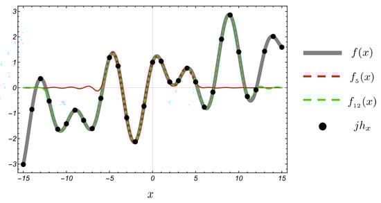
Figure 2. The effect of the choice of $N_x$ on the approximation $f\left(x\right)\approx f_{Nx}\left(x\right)$ in (3).

Note that Equation (2) is focused on the interval $[a,b]\subset \mathbb{R}$. To transform the basis functions on the interval $(a,b)$, we consider a conformal map, which is a complex function that preserves angles locally, that is, it is analytic and its derivative never vanishes [27]. We take the conformal map [24,25]

$$w=\varphi \left(z\right)=ln\left({\displaystyle \frac{z-a}{b-z}}\right),$$

which transforms the simple connected region (see Figure 3)

$${\mathcal{D}}_E=\left\{z\in \mathbb{C}:\left|arg\left({\displaystyle \frac{z-a}{b-z}}\right)\right|<d\mathrm{and}0<d\le {\displaystyle \frac{\pi }{2}}\right\},$$

to the strip-shaped region ${\mathcal{D}}_d$. In this case, the branch of the logarithm is chosen such that the argument of $(z-a)/(b-z)$ is restricted to $(-d,d)$, mapping the boundaries of the z-domain to the lines $\mathrm{Im}\left(w\right)=\pm d$ (see Figure 3). It is easy to check that

$$z={\varphi }^{-1}\left(w\right)={\displaystyle \frac{a+b{e}^w}{1+e^w}}.$$

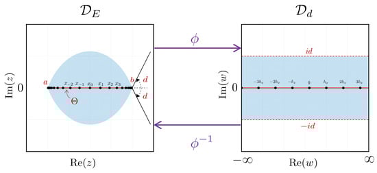
Figure 3. Illustration of the eye-shaped region ${\mathcal{D}}_E$ the strip-shaped region ${\mathcal{D}}_d$ with the corresponding conformal map $\varphi$ and its inverse ${\varphi }^{-1}$.

Note that $a,b\in \partial {\mathcal{D}}_E$, i.e., on the boundary of ${\mathcal{D}}_E$, with $a={\varphi }^{-1}(-\infty )$ and $b={\varphi }^{-1}(\infty )$. Consequently, we set (see Figure 3)

$$\mathrm{\Theta }=\{{\varphi }^{-1}\left(\eta \right):\eta \in \mathbb{R}\}\subset {\mathcal{D}}_E.$$

Let $h_x>0$ and consider the uniformly distributed points ${\left\{j{h}_x\right\}}_{j\in \mathbb{Z}}\subset {\mathcal{D}}_d$ on the real line. Then, the corresponding points $x_j\in \mathrm{\Theta }$ are (see Figure 3)

$$x_j={\varphi }^{-1}\left(j{h}_x\right)={\displaystyle \frac{a+b{e}^{j{h}_x}}{1+e^{j{h}_x}}},j\in \mathbb{Z}.$$

Hence, the basis functions on $(a,b)$ are

$${\mathcal{S}}_j\left(z\right)=\mathcal{S}(j,h_x)\left(x\right)\circ \varphi \left(z\right)=\mathrm{sinc}\left({\displaystyle \frac{\varphi \left(z\right)-j{h}_x}{h_x}}\right),j\in \mathbb{Z}.$$

(4)

Note that these $\mathrm{sinc}$ functions satisfy

$${\delta }_{jk}^{\left(p\right)}=h_x^p{\left.{\displaystyle \frac{d^p{S}_j\left(x\right)}{d{x}^p}}\right|}_{x=x_k},p=0,1,2,\dots .$$

In particular, we have

$$\begin{array}{cc}{\delta }_{jk}^{\left(0\right)}\hfill & ={\mathcal{S}}_j\left(x_k\right)=\left\{\begin{array}{cc}1,\hfill & \mathrm{if}j=k,\hfill \\ 0,\hfill & \mathrm{if}j\ne k,\hfill \end{array}\right.\hfill \\ {\delta }_{jk}^{\left(1\right)}\hfill & =h_x{\left.{\displaystyle \frac{d{S}_j\left(x\right)}{dx}}\right|}_{x=x_k}=\left\{\begin{array}{cc}0,& \mathrm{if}j=k,\hfill \\ {\displaystyle \frac{{(-1)}^{k-j}}{k-j}},& \mathrm{if}j\ne k,\hfill \end{array}\right.\hfill \\ {\delta }_{jk}^{\left(2\right)}\hfill & =h_x^2{\left.{\displaystyle \frac{d^2{S}_j\left(x\right)}{d{x}^2}}\right|}_{x=x_k}=\left\{\begin{array}{cc}{\displaystyle \frac{-{\pi }^2}{3}},& \mathrm{if}j=k,\hfill \\ {\displaystyle \frac{-2{(-1)}^{k-j}}{{(k-j)}^2}},& \mathrm{if}j\ne k.\hfill \end{array}\right.\hfill \end{array}$$

(5)

To approximate the function f by a finite series on $(a,b)$ using $\mathrm{sinc}$ functions in (4)

$$f\left(x\right)\approx f_{N_x}\left(x\right)=\sum _{j=-N_x}^{N_x}f\left(x_j\right){\mathcal{S}}_j\left(x\right),$$

(6)

we provide the following conditions on f to guarantee convergence.

Definition 1 

([24]). Let $\kappa >0$, $\Sigma =\left\{iy:\left|y\right|<d\mathit{and}0<d\le {\displaystyle \frac{\pi }{2}}\right\}$ and for $f:{\mathcal{D}}_E\to \mathbb{C}$ set

$${\mathcal{P}}_t\left(f\right)={\int }_{{\varphi }^{-1}(t+\Sigma )}\left|f\left(z\right)\right|\mathrm{d}zand\mathcal{Q}\left(f\right)={\int }_{\partial {\mathcal{D}}_E}\left|f\left(z\right)\mathrm{d}z\right|.$$

Here, $t+\Sigma =\left\{z\in \mathbb{C}:\mathrm{Re}\left(z\right)=t\mathit{and}i\mathrm{Im}\left(z\right)\in \Sigma \right\}$. Then, we define the following families of functions ${\mathrm{B}}_1\left({\mathcal{D}}_E\right)$ and ${\mathrm{B}}_2\left({\mathcal{D}}_E\right)$ on ${\mathcal{D}}_E$:

$$\begin{array}{cc}\hfill {\mathrm{B}}_1\left({\mathcal{D}}_E\right)& =\left\{f:{\mathcal{D}}_E\to \mathbb{C}:f\mathit{is}\mathit{analytic},\underset{t\to \infty }{lim}{\mathcal{P}}_t\left(f\right)=0,\mathit{and}\mathcal{Q}\left(f\right)<\infty \right\},\hfill \\ \hfill {\mathrm{B}}_2\left({\mathcal{D}}_E\right)& =\left\{f:{\mathcal{D}}_E\to \mathbb{C}:f\mathit{is}\mathit{analytic},\left|f\left(z\right)\right|\le C_0{e}^{-\kappa \left|\varphi \right(x\left)\right|}\mathit{for}\mathit{some}{C}_0\in {\mathbb{R}}_{+}\right\}.\hfill \end{array}$$

The following theorem provides an approximation of the p-derivative of $f\left(x\right)$ [25].

Theorem 1. 

If the conformal map ϕ is one-to-one and $f\left(x\right),{\varphi }^{\prime }\left(x\right)\in {\mathrm{B}}_1\left({\mathcal{D}}_E\right)$. Then, for all $x\in \mathrm{\Theta }$, we have

$$\left|f\left(x\right)-\sum _{j=-N_x}^{N_x}f\left(x_j\right)S_j\left(x\right)\right|\le {\displaystyle \frac{2\mathcal{Q}\left(f{\varphi }^{\prime }\right)}{\pi d}}{e}^{-\pi d/h_x}.$$

Moreover, when $f\left(x\right)\in {\mathrm{B}}_2\left({\mathcal{D}}_E\right)$ and $h_x=\sqrt{{\displaystyle \frac{\pi d}{\kappa N_x}}}$, then there exists $C_1\in {\mathbb{R}}_{+}$ such that

$$\begin{array}{c}\hfill \underset{x\in \mathrm{\Theta }}{sup}\left|{\displaystyle \frac{d^{p}f\left(x\right)}{d{x}^p}}-\sum _{j=-N_x}^{N_x}f\left(x_j\right){\displaystyle \frac{d^p{\mathcal{S}}_j\left(x\right)}{d{x}^p}}\right|\le C_1{N}_x^{(p+1)/2}{e}^{-\sqrt{\pi \kappa d{N}_x}},\end{array}$$

for $p=0,1,2,\dots$. The constant $C_1$ depends on p, ϕ, d, κ, and f.

Note that Theorem 1 provides an approximation of the p-derivative of $f\left(x\right)$ with an exponential convergent, that is,

$${\displaystyle \frac{d^{p}f\left(x\right)}{d{x}^p}}=\sum _{j=-N_x}^{N_x}f\left(x_j\right){\displaystyle \frac{d^p{\mathcal{S}}_j\left(x\right)}{d{x}^p}}+\mathcal{O}\left(N_x^{(p+1)/2}{e}^{-\sqrt{\pi \kappa d{N}_x}}\right).$$

Recall that ${\mathcal{S}}_j\left(z\right)=\mathcal{S}(j,h_x)\left(x\right)\circ \varphi \left(z\right)$. Hence, at $x=x_k$, we have

$${\displaystyle \frac{d^{2}f\left(x_k\right)}{d{x}^2}}\approx \sum _{j=-N_x}^{N_x}\left({\displaystyle \frac{1}{h_x}}{\delta }_{jk}^{\left(1\right)}{\varphi }^{″}\left(x_k\right)+{\displaystyle \frac{1}{h_x^2}}{\delta }_{jk}^{\left(2\right)}{\left({\varphi }^{\prime }\left(x_k\right)\right)}^2\right)f\left(x_j\right).$$

(7)

Let $m_x=2N_x+1$. To help represent discrete systems, we define the column vectors

$$\begin{array}{cc}\hfill \mathbf{F}\left(X\right)& ={\left[f\left(x_{-Nx}\right),\dots ,f\left(x_{Nx}\right)\right]}^T,\hfill \\ \hfill {\displaystyle \frac{d^2\mathbf{F}\left(X\right)}{d{x}^2}}& ={\left[{\displaystyle \frac{d^{2}f\left(x_{-Nx}\right)}{d{x}^2}},\dots ,{\displaystyle \frac{d^{2}f\left(x_{Nx}\right)}{d{x}^2}}\right]}^T,\hfill \end{array}$$

where $\mathbf{X}={[x_{-N_x},\dots ,x_{N_x}]}^T$, and the following $m_x\times m_x$ matrices, the diagonal matrix

$$\mathbf{D}\left(g\right)=\mathrm{diag}\left[g\left(x_{-N_x}\right),\dots ,g\left(x_{Nx}\right)\right],$$

and using (5), we have

$${\mathbf{I}}^{\left(p\right)}={\left[{\delta }_{jk}^{\left(p\right)}\right]}_{j,k=-N_x}^{N_x},p=0,1,2.$$

The matrix ${\mathbf{I}}^{\left(0\right)}$ is the identity matrix, ${\mathbf{I}}^{\left(1\right)}$ is the skew symmetric Toeplitz matrix

$${\mathbf{I}}^{\left(1\right)}=\left[\begin{array}{cccccc}0& -1& {\displaystyle \frac{1}{2}}& -{\displaystyle \frac{1}{3}}& \dots & {\displaystyle \frac{{(-1)}^{m_x-1}}{m_x-1}}\\ 1& 0& -1& {\displaystyle \frac{1}{2}}& \dots & -{\displaystyle \frac{{(-1)}^{m_x-2}}{m_x-2}}\\ -{\displaystyle \frac{1}{2}}& 1& 0& -1& \dots & {\displaystyle \frac{{(-1)}^{m_x-3}}{m_x-3}}\\ {\displaystyle \frac{1}{3}}& -{\displaystyle \frac{1}{2}}& 1& 0& \dots & -{\displaystyle \frac{{(-1)}^{m_x-4}}{m_x-4}}\\ ⋮& ⋮& ⋮& ⋮& \ddots & ⋮\\ -{\displaystyle \frac{{(-1)}^{m_x-1}}{m_x-1}}& {\displaystyle \frac{{(-1)}^{m_x-2}}{m_x-2}}& -{\displaystyle \frac{{(-1)}^{m_x-3}}{m_x-3}}& {\displaystyle \frac{{(-1)}^{m_x-4}}{m_x-4}}& \dots & 0\end{array}\right]$$

and ${\mathbf{I}}^{\left(2\right)}$ is and the symmetric Toeplitz matrix

$${\mathbf{I}}^{\left(2\right)}=\left[\begin{array}{cccccc}-{\displaystyle \frac{{\pi }^2}{3}}& 2& -{\displaystyle \frac{1}{2}}& {\displaystyle \frac{2}{9}}& \dots & {\displaystyle \frac{-2{(-1)}^{m_x-1}}{{(m_x-1)}^2}}\\ 2& -{\displaystyle \frac{{\pi }^2}{3}}& 2& -{\displaystyle \frac{1}{2}}& \dots & {\displaystyle \frac{-2{(-1)}^{m_x-2}}{{(m_x-2)}^2}}\\ -{\displaystyle \frac{1}{2}}& 2& -{\displaystyle \frac{{\pi }^2}{3}}& 2& \dots & {\displaystyle \frac{-2{(-1)}^{m_x-3}}{{(m_x-1)}^3}}\\ {\displaystyle \frac{2}{9}}& -{\displaystyle \frac{1}{2}}& 2& -{\displaystyle \frac{{\pi }^2}{3}}& \dots & {\displaystyle \frac{-2{(-1)}^{m_x-4}}{{(m_x-1)}^4}}\\ ⋮& ⋮& ⋮& ⋮& \ddots & ⋮\\ {\displaystyle \frac{-2{(-1)}^{m_x-1}}{{(m_x-1)}^2}}& {\displaystyle \frac{-2{(-1)}^{m_x-2}}{{(m_x-2)}^2}}& {\displaystyle \frac{-2{(-1)}^{m_x-3}}{{(m_x-1)}^3}}& {\displaystyle \frac{-2{(-1)}^{m_x-4}}{{(m_x-1)}^4}}& \dots & -{\displaystyle \frac{{\pi }^2}{3}}\end{array}\right].$$

Hence, we can write Equation (7) as

$${\displaystyle \frac{d^2\mathbf{F}\left(\mathbf{X}\right)}{d{x}^2}}\approx \left[{\displaystyle \frac{1}{h_x}}\mathbf{D}\left({\varphi }^{″}\right){\mathbf{I}}^{\left(1\right)}+{\displaystyle \frac{1}{h_x^2}}\mathbf{D}\left({\left({\varphi }^{\prime }\right)}^2\right){\mathbf{I}}^{\left(1\right)}\right]\mathbf{F}\left(\mathbf{X}\right).$$

(8)

Consequently, we approximate $u_{xx}(x,t)$ in (2) by (7) or (8)

$$u_{xx}(x_k,t)\approx \sum _{j=-N_x}^{N_x}\left({\displaystyle \frac{1}{h_x}}{\delta }_{jk}^{\left(1\right)}{\varphi }^{″}\left(x_k\right)+{\displaystyle \frac{1}{h_x^2}}{\delta }_{jk}^{\left(2\right)}{\left({\varphi }^{\prime }\left(x_k\right)\right)}^2\right)u(x_j,t),$$

(9)

or

$${\mathbf{U}}_{xx}(\mathbf{X},t)\approx \left[{\displaystyle \frac{1}{h_x}}\mathbf{D}\left({\varphi }^{″}\right){\mathbf{I}}^{\left(1\right)}+{\displaystyle \frac{1}{h_x^2}}\mathbf{D}\left({\left({\varphi }^{\prime }\right)}^2\right){\mathbf{I}}^{\left(1\right)}\right]\mathbf{U}(\mathbf{X},t),$$

(10)

respectively, where

$$\begin{array}{cc}\hfill \mathbf{U}(\mathbf{X},t)& ={\left[u(x_{-N_x},t),\dots ,u(x_{N_x},t)\right]}^T,\hfill \\ \hfill {\mathbf{U}}_{xx}(\mathbf{X},t)& ={\left[u_{xx}(x_{-N_x},t),\dots ,u_{xx}(x_{N_x},t)\right]}^T.\hfill \end{array}$$

3. The Temporal Discretization

In this section, we approximate the time-fractional derivative and integral term in (2). Let $N_t\in {\mathbb{Z}}_{+}$ and set $\Delta t=T/N_t$. Denote $t_n=n\Delta t$, $u^n=u\left(x,t_n\right)$, and $H^n=H\left(x,t_n\right)$ for $n=0,\dots ,N_t$.

To approximate the time-fractional derivative in (2), we use the weighted and shifted Grünwald difference (WSGD) operator. Suppose that $\psi \left(t\right)\in L_1\left(\mathbb{R}\right)$ and $\psi \left(t\right)\in C^{\alpha +1}\left(\mathbb{R}\right)$. Then, the shifted Grünwald difference operator is defined by [28]

$$G_{\Delta t,m}^{\alpha }\psi \left(t\right)={\displaystyle \frac{1}{\Delta t^{\alpha }}}\sum _{i=0}^{\infty }{\xi }_i^{\left(\alpha \right)}\psi (t-(i-m)\Delta t),$$

where $m\in \mathbb{Z}$ and the coefficients ${\xi }_i^{\left(\alpha \right)}$ can be evaluated recursively as

$${\xi }_0^{\left(\alpha \right)}=1,{\xi }_i^{\left(\alpha \right)}=\left(1-{\displaystyle \frac{\alpha +1}{i}}\right){\xi }_{i-1}^{\alpha },i=1,2,\cdots .$$

Moreover, we have

$$G_{\Delta t,m}^{\alpha }\psi \left(t\right)=D_t^{\alpha }\psi \left(t\right)+O(\Delta t)$$

uniformly for $t\in \mathbb{R}$ as $\Delta t\to 0$.

Theorem 2

 ([29]). Assume $\psi \left(t\right)$, $D_t^{\alpha +2}\psi \left(t\right)$, and $\mathcal{F}\left\{D_t^{\alpha +2}\psi \right\}$ belong to the Lebesgue space $L_1\left(\mathbb{R}\right)$, where $\mathcal{F}$ denotes the Fourier transform. Then, the weighted and shifted Grünwald difference operator is defined by

$$D_{\Delta t,m,r}^{\alpha }\psi \left(t\right)={\displaystyle \frac{2r-\alpha }{2(r-m)}}{G}_{\Delta t,m}^{\alpha }\psi \left(t\right)+{\displaystyle \frac{2m-\alpha }{2(m-r)}}{G}_{\Delta t,r}^{\alpha }\psi \left(t\right),$$

where m and r are integers such that $m\ne r$. Then,

$$D_{\Delta t,m,r}^{\alpha }\psi \left(t\right)=D_t^{\alpha }\psi \left(t\right)+O\left(\Delta t^2\right),$$

uniformly for $t\in \mathbb{R}$ as $\Delta t\to 0$. Furthermore, the m and r are symmetric, that is, ${\mathcal{D}}_{\Delta t,m,r}^{\alpha }={\mathcal{D}}_{\Delta t,r,m}^{\alpha }$.

Theorem 2 implies that the discrete approximations for Riemann–Liouville fractional derivatives when $0<\alpha <1$ is simplified as [30]:

$$\begin{array}{cc}{D}_t^{\alpha }u\left(x,t_n\right)\hfill & ={\displaystyle \frac{1}{\Delta t^{\alpha }}}\left(\left(1+{\displaystyle \frac{\alpha }{2}}\right){\displaystyle \sum _{i=0}^n}{\xi }_i^{\left(\alpha \right)}u(x,t_{n-i})-{\displaystyle \frac{\alpha }{2}}{\displaystyle \sum _{i=0}^{n-1}}{\xi }_i^{\left(\alpha \right)}u(x,t_{n-i-1})\right)+O\left(\Delta t^2\right)\\ & ={\displaystyle \frac{1}{\Delta t^{\alpha }}}{\displaystyle \sum _{i=0}^n}{w}_i^{\left(\alpha \right)}u(x,t_{n-i})+{\tilde{E}}_{n+1},\hfill \end{array}$$

(11)

where ${\tilde{E}}_{n+1}=O\left(\Delta t^2\right)$ and

$$\begin{array}{ccc}& w_0^{\left(\alpha \right)}=\left(1+{\displaystyle \frac{\alpha }{2}}\right){\xi }_0^{\left(\alpha \right)}=1+{\displaystyle \frac{\alpha }{2}},\hfill & \hfill w_k^{\left(\alpha \right)}=\left(1+{\displaystyle \frac{\alpha }{2}}\right){\xi }_i^{\left(\alpha \right)}-{\displaystyle \frac{\alpha }{2}}{\xi }_{i-1}^{\left(\alpha \right)},i\ge 1.\end{array}$$

For the integral term in (2) involving the weakly singular kernel, we use a quadrature approximation based on a product trapezoidal integration rule [31,32]. For $n=0,\dots ,N_t-1$, we have

$$\begin{array}{cc}\hfill & {\int }_0^{t_{n+1}}{\left(t_{n+1}-s\right)}^{\beta -1}{u}_{xx}(x,s)ds=\sum _{i=0}^n{\int }_{t_i}^{t_{i+1}}{\left(t_{n+1}-s\right)}^{\beta -1}{u}_{xx}(x,s)ds\hfill \\ \hfill & =\sum _{i=0}^n{\int }_{t_i}^{t_{i+1}}{\left(t_{n+1}-s\right)}^{\beta -1}\left({\displaystyle \frac{t_{i+1}-s}{\Delta t}}{u}_{xx}(x,t_i)+{\displaystyle \frac{s-t_i}{\Delta t}}{u}_{xx}(x,t_{i+1})\right)ds+{\widehat{E}}_{n+1}\hfill \\ \hfill & ={\displaystyle \frac{1}{\Delta t}}\sum _{i=0}^n\left(P_{n,i}{u}_{xx}(x,t_i)\left(x\right)+Q_{n,i}{u}_{xx}(x,t_{i+1})\right)+{\widehat{E}}_{n+1},\hfill \end{array}$$

where

$$\begin{array}{ccc}\hfill & P_{n,i}={\int }_{t_i}^{t_{i+1}}{\left(t_{n+1}-s\right)}^{\beta -1}\left(t_{i+1}-s\right)ds,\hfill & \hfill Q_{n,i}={\int }_{t_i}^{t_{i+1}}{\left(t_{n+1}-s\right)}^{\beta -1}\left(s-t_i\right)ds,\end{array}$$

and ${\widehat{E}}_{n+1}=\mathcal{O}\left(\Delta t^{1+\beta }\right)$ is the order of the product trapezoidal integration rule [32]. Consequently, we have

$${\int }_0^{t_{n+1}}{\left(t_{n+1}-s\right)}^{\beta -1}{u}_{xx}(x,s)ds={\displaystyle \frac{1}{\Delta t}}\left(Q_{n,n}{u}_{xx}(x,t_{n+1})+\sum _{i=0}^n{\Lambda }_{n,i}{u}_{xx}(x,t_i)\right)+{\widehat{E}}_{n+1},$$

(12)

where

$$\begin{array}{c}\hfill {\Lambda }_{n,0}=P_{n,0},{\Lambda }_{n,i}=P_{n,i}+Q_{n,i-1},i=1,2,\dots ,n.\end{array}$$

Substituting Equations (11) and (12) into Equation (2) leads to a temporal semi-discrete form of Equation (2) as follows:

$$\begin{array}{cc}\hfill & w_0^{\left(\alpha \right)}u(x,t_{n+1})-\left(\Delta t^{\alpha }+\Delta t^{\alpha -1}{Q}_{n,n}\right)u_{xx}(x,t_{n+1})\hfill \\ \hfill =& \Delta t^{\alpha -1}\sum _{i=0}^n{\Lambda }_{n,i}{u}_{xx}(x,t_i)-\sum _{i=1}^{n+1}{w}_i^{\left(\alpha \right)}u(x,t_{n+1-i})+\Delta t^{\alpha }H(x,t_{n+1})+E_{n+1},\hfill \end{array}$$

where $E_{n+1}\le min\{{\tilde{E}}_{n+1},{\widehat{E}}_{n+1}\}$. Dropping the error term $E_{n+1}$, we obtain

$$\begin{array}{cc}\hfill & w_0^{\left(\alpha \right)}u(x,t_{n+1})-\left(\Delta t^{\alpha }+\Delta t^{\alpha -1}{Q}_{n,n}\right)u_{xx}(x,t_{n+1})\hfill \\ \hfill =& \Delta t^{\alpha -1}\sum _{i=0}^n{\Lambda }_{n,i}{u}_{xx}(x,t_i)-\sum _{i=1}^{n+1}{w}_i^{\left(\alpha \right)}u(x,t_{n+1-i})+\Delta t^{\alpha }H(x,t_{n+1}),\hfill \end{array}$$

(13)

with $u(a,t_{n+1})=0$, $u(b,t_{n+1})=0$, and $u(x,0)=g\left(x\right)$. Suppose that the approximate solution to Equation (13) using Equation (9) is given by

$$v_{\mathrm{app}}(x,t_n)=\sum _{j=-N_x}^{N_x}{v}_j^n{\mathcal{S}}_j\left(x\right).$$

(14)

At $x=x_k$, denote $H_k^n=H\left(x_k,t_n\right)$ for $n=0,\dots ,N_t$. Now, substituting $v_{\mathrm{app}}(x,t_n)$ in Equation (13) leads to

$$\begin{array}{cc}\hfill & w_0^{\left(\alpha \right)}\sum _{j=-N_x}^{N_x}{v}_k^{n+1}{\delta }_{jk}^{\left(0\right)}-\left(\Delta t^{\alpha }+\Delta t^{\alpha -1}{Q}_{n,n}\right)\sum _{j=-N_x}^{N_x}{v}_k^{n+1}\left[{\varphi }^{″}\left(x_k\right){\displaystyle \frac{{\delta }_{jk}^{\left(1\right)}}{h_x}}+{\left({\varphi }^{\prime }\left(x_k\right)\right)}^2{\displaystyle \frac{{\delta }_{jk}^{\left(2\right)}}{h_x^2}}\right]\hfill \\ \hfill =& \Delta t^{\alpha -1}\sum _{i=0}^n\sum _{j=-N_x}^{N_x}{\Lambda }_{n,i}{v}_k^i\left[{\varphi }^{″}\left(x_k\right){\displaystyle \frac{{\delta }_{jk}^{\left(1\right)}}{h_x}}+{\left({\varphi }^{\prime }\left(x_k\right)\right)}^2{\displaystyle \frac{{\delta }_{jk}^{\left(2\right)}}{h_x^2}}\right]-\sum _{i=1}^{n+1}\sum _{j=-N_x}^{N_x}{w}_i^{\left(\alpha \right)}{v}_k^{n+1-i}{\delta }_{jk}^{\left(0\right)}+\Delta t^{\alpha }{H}_i^{n+1},\hfill \end{array}$$

(15)

with initial condition $v_j^0=g\left(x_j\right)$. Multiplying Equation (15) by ${\displaystyle \frac{1}{{\left({\varphi }^{\prime }\left(x_k\right)\right)}^2}}$ gives

$$\begin{array}{cc}\hfill & {\displaystyle \frac{w_0^{\left(\alpha \right)}}{{\left({\varphi }^{\prime }\left(x_k\right)\right)}^2}}{v}_k^{n+1}-\left(\Delta t^{\alpha }+\Delta t^{\alpha -1}{Q}_{n,n}\right)\sum _{j=-N_x}^{N_x}{v}_k^{n+1}\left[{\displaystyle \frac{{\varphi }^{″}\left(x_k\right)}{{\left({\varphi }^{\prime }\left(x_k\right)\right)}^2}}{\displaystyle \frac{{\delta }_{jk}^{\left(1\right)}}{h_x}}+{\displaystyle \frac{{\delta }_{jk}^{\left(2\right)}}{h_x^2}}\right]\hfill \\ \hfill =& \Delta t^{\alpha -1}\sum _{i=1}^{n+1}\sum _{j=-N_x}^{N_x}{\Lambda }_{n,i}{v}_k^i\left[{\displaystyle \frac{{\varphi }^{″}\left(x_k\right)}{{\left({\varphi }^{\prime }\left(x_k\right)\right)}^2}}{\displaystyle \frac{{\delta }_{jk}^{\left(1\right)}}{h_x}}+{\displaystyle \frac{{\delta }_{jk}^{\left(2\right)}}{h_x^2}}\right]\hfill \\ \hfill & -{\displaystyle \frac{1}{{\left({\varphi }^{\prime }\left(x_k\right)\right)}^2}}\sum _{i=1}^{n+1}\sum _{j=-N_x}^{N_x}{w}_i^{\left(\alpha \right)}{v}_k^{n+1-i}{\delta }_{jk}^{\left(0\right)}+{\displaystyle \frac{\Delta t^{\alpha }}{{\left({\varphi }^{\prime }\left(x_k\right)\right)}^2}}{H}_i^{n+1}.\hfill \end{array}$$

(16)

Let

$$\begin{array}{c}\hfill {\mathbf{V}}^n={\left[v_{-N_x}^n,v_{-N_x+1}^n,\dots ,v_{N_x}^n\right]}^{\mathrm{T}},\\ \hfill {\mathbf{H}}^n={\left[H_{-N_x}^n,H_{-N_x+1}^n,\dots ,H_{N_x}^n\right]}^{\mathrm{T}}.\end{array}$$

Then, the matrix form of Equation (16) is

$$\begin{array}{cc}\hfill & w_0^{\left(\alpha \right)}\mathbf{D}\left[{\displaystyle \frac{1}{{\left({\varphi }^{\prime }\right)}^2}}\right]{\mathbf{V}}^{n+1}-\left(\Delta t^{\alpha }+\Delta t^{\alpha -1}{Q}_{n,n}\right)\left[{\displaystyle \frac{1}{h_x}}\mathbf{D}{\left({\displaystyle \frac{1}{{\varphi }^{\prime }}}\right)}^{\prime }{\mathbf{I}}^{\left(1\right)}+{\displaystyle \frac{1}{h_x^2}}{\mathbf{I}}^{\left(2\right)}\right]{\mathbf{V}}^{n+1}\hfill \\ \hfill & =\Delta t^{\alpha -1}\sum _{i=0}^n{\Lambda }_{n,i}\left[{\displaystyle \frac{1}{h_x}}\mathbf{D}{\left({\displaystyle \frac{1}{{\varphi }^{\prime }}}\right)}^{\prime }{\mathbf{I}}^{\left(1\right)}+{\displaystyle \frac{1}{h_x^2}}{\mathbf{I}}^{\left(2\right)}\right]{\mathbf{V}}^i+\Delta t^{\alpha }\mathbf{D}\left[{\displaystyle \frac{1}{{\left({\varphi }^{\prime }\right)}^2}}\right]{\mathbf{H}}^{n+1}\hfill \\ \hfill +& \mathbf{D}\left[{\displaystyle \frac{1}{{\left({\varphi }^{\prime }\right)}^2}}\right]\left(w_1^{\left(\alpha \right)}{\mathbf{V}}^n+w_2^{\left(\alpha \right)}{\mathbf{V}}^{n-1}+\dots +w_n^{\left(\alpha \right)}{\mathbf{V}}^1+w_{n+1}^{\left(\alpha \right)}{\mathbf{V}}^0\right).\hfill \end{array}$$

Consequently, we write it as

$${\mathbf{M}}_3{\mathbf{V}}^{n+1}={\mathbf{M}}_1\left({\displaystyle \frac{\Delta t^{\alpha }}{w_0^{\left(\alpha \right)}}}{\mathbf{H}}^{n+1}+{\displaystyle \frac{1}{w_0^{\left(\alpha \right)}}}\sum _{i=0}^n{w}_{n+1-i}^{\left(\alpha \right)}{\mathbf{V}}^i\right)+{\displaystyle \frac{\Delta t^{\alpha -1}}{w_0^{\left(\alpha \right)}}}\sum _{i=0}^n{\Lambda }_{n,i}{\mathbf{M}}_2{\mathbf{V}}^i,$$

(17)

where

$${\mathbf{M}}_1=\mathbf{D}\left[{\displaystyle \frac{1}{{\left({\varphi }^{\prime }\right)}^2}}\right],{\mathbf{M}}_2={\displaystyle \frac{1}{h_x}}\mathbf{D}{\left({\displaystyle \frac{1}{{\varphi }^{\prime }}}\right)}^{\prime }{\mathbf{I}}^{\left(1\right)}+{\displaystyle \frac{1}{h_x^2}}{\mathbf{I}}^{\left(2\right)},{\mathbf{M}}_3={\mathbf{M}}_1-Q_{n,n}{\mathbf{M}}_2.$$

(18)

Denote

$${\mathrm{\Psi }}^{n+1}={\mathbf{M}}_1\left({\displaystyle \frac{\Delta t^{\alpha }}{w_0^{\left(\alpha \right)}}}{\mathbf{H}}^{n+1}+{\displaystyle \frac{1}{w_0^{\left(\alpha \right)}}}\sum _{i=0}^n{w}_{n+1-i}^{\left(\alpha \right)}{\mathbf{V}}^i\right)+{\displaystyle \frac{\Delta t^{\alpha -1}}{w_0^{\left(\alpha \right)}}}\sum _{i=0}^n{\Lambda }_{n,i}{\mathbf{M}}_2{\mathbf{V}}^i.$$

Then, Equation (17) can be written as the iteration form

$${\mathbf{M}}_3{\mathbf{V}}^{n+1}={\mathrm{\Psi }}^{n+1},$$

(19)

with the initial condition

$${\mathbf{V}}^0={\left[g\left(x_{-N_x}\right),g\left(x_{-N_x+1}\right),\dots ,g\left(x_{N_x}\right)\right]}^{\mathrm{T}}.$$

For each $n\in \{0,\dots ,N_t-1\}$, the iteration Equation (19) forms a system of $2N_x+1$ linear equations and $2N_x+1$ variables. The coefficients of the approximate solution in Equation (14) can be obtained by solving this system.

Note that due to its diagonal shape and strictly positive entries, the matrix ${\mathbf{M}}_1$ is invertible and positive definite. A discretized second derivative gives rise to the symmetric positive semi-definite matrix ${\mathbf{M}}_2$. Since the coefficient $Q_{n,n}$ is small for sufficiently small time steps $\Delta t$, the matrix ${\mathbf{M}}_3$ is a minor perturbation of a positive definite matrix. Thus, ${\mathbf{M}}_3$ is, therefore, invertible, and hence, Equation (19) has a unique solution ${\mathbf{V}}^{n+1}={\mathbf{M}}_3^{-1}{\mathrm{\Psi }}^{n+1}$.

4. Stability and Convergence Analysis

Now, we analyze the convergence of the iteration Equation (19) for the FPIDE Equation (2). To this end, we rewrite, for simplicity, Equation (13) as an ordinary differential equation

$$w_0^{\left(\alpha \right)}{u}^{n+1}\left(x\right)-\left(\Delta t^{\alpha }+\Delta t^{\alpha -1}{Q}_{n,n}\right){\displaystyle \frac{d^2{u}^{n+1}\left(x\right)}{d{x}^2}}=\mathrm{\Phi }\left(x\right),$$

(20)

where

$$\mathrm{\Phi }\left(x\right)=\Delta t^{\alpha -1}\sum _{i=0}^n{\Lambda }_{n,i}{\displaystyle \frac{d^2{u}^i\left(x\right)}{d{x}^2}}-\sum _{i=1}^{n+1}{w}_i^{\left(\alpha \right)}{u}^{n+1-i}\left(x\right)+\Delta t^{\alpha }H(x,t_{n+1})$$

taking into account the boundary conditions $u^{n+1}\left(0\right)=u^{n+1}\left(1\right)=0$. Suppose that $u^{n+1}\left(x\right)$ is the exact solution of Equation (20), which satisfies Equation (2) at the $(n+1)$-th time step. Assume that $u_{\mathrm{app}}^{n+1}\left(x\right)$ be the approximate solution of Equation (20) using the $\mathrm{sinc}$-collocation formula in Equation (14). At $x=x_j$, the solution of Equation (2) is computed by

$$u_{\mathrm{pt}}^{n+1}\left(x\right)=\sum _{j=-N_x}^{N_x}{u}^{n+1}\left(x_j\right)S_j\left(x\right).$$

(21)

In the following, we first determine a suitable upper bound for $\left|u_{\mathrm{app}}^{n+1}-u_{\mathrm{pt}}^{n+1}\left(x\right)\right|$, then we establish an upper bound for $\left|u^{n+1}\left(x\right)-u_{\mathrm{app}}^{n+1}\left(x\right)\right|$.

The following result from [33] provides the necessary upper bound for ${∥{\mathbf{M}}_3^{-1}∥}_2$.

Theorem 3. 

Denote ${\mathbf{M}}_3^{*}$ by the conjugate transpose of the matrix ${\mathbf{M}}_3$ in Equation (17). Let $x\in \mathrm{\Theta }$, then we have

$${\displaystyle \frac{{\mathbf{M}}_3+{\mathbf{M}}_3^{*}}{2}}=\mathrm{\Pi }-{\displaystyle \frac{Q_{n,n}}{h_x^2}}{\mathbf{I}}^{\left(2\right)},$$

where

$$\mathrm{\Pi }=\mathbf{D}\left(Re\left({\left({\displaystyle \frac{1}{{\varphi }^{\prime }}}\right)}^2\right)\right)-{\displaystyle \frac{Q_{n,n}}{2h_x}}\left[\mathbf{D}\left({\left({\displaystyle \frac{1}{{\varphi }^{\prime }}}\right)}^{\prime }\right){\mathbf{I}}^{\left(1\right)}-{\mathbf{I}}^{\left(1\right)}\mathbf{D}\left({\left(\overline{{\displaystyle \frac{1}{{\varphi }^{\prime }}}}\right)}^{\prime }\right)\right].$$

Moreover, if the eigenvalues of the matrix $\mathrm{\Pi }$ are nonnegative, then there exists $C_0$, which is independent of $N_x$, such that for a sufficiently large $N_x$, we have

$${∥{\mathbf{M}}_3^{-1}∥}_2\le {\displaystyle \frac{4d{N}_x}{\kappa \pi Q_{n,n}}}\left(1+{\displaystyle \frac{C_0}{N_x}}\right).$$

(22)

Note that Theorem 3 implies that the matrix ${∥{\mathbf{M}}_3^{-1}∥}_2$ is bounded as long as $Q_{n,n}$ does not vanish and $N_x$ is sufficiently large. Consistently, we have the following result.

Theorem 4. 

The numerical scheme in Equation (19) is stable.

Proof. 

Suppose that ${\mathrm{\Psi }}^{n+1}$, with solution ${\mathbf{V}}^{n+1}$ in Equation (19), contains a small error $\epsilon \mathrm{\Psi }$. Denote ${\tilde{\mathrm{\Psi }}}^{n+1}={\mathrm{\Psi }}^{n+1}+\epsilon {\mathrm{\Psi }}^{n+1}$ and the corresponding solution ${\tilde{\mathbf{V}}}^{n+1}$. Hence, Equation (19) gives

$${\mathbf{M}}_3{\tilde{\mathbf{V}}}^{n+1}={\tilde{\mathrm{\Psi }}}^{n+1}.$$

Note that

$${\tilde{\mathrm{\Psi }}}^{n+1}={\mathbf{M}}_3{\mathbf{V}}^{n+1}+\epsilon {\mathrm{\Psi }}^{n+1}.$$

Thus,

$${\mathbf{M}}_3({\tilde{\mathbf{V}}}^{n+1}-{\mathbf{V}}^{n+1})=\epsilon {\mathrm{\Psi }}^{n+1}.$$

Define the error $\epsilon {\mathbf{V}}^{n+1}:={\tilde{V}}^{n+1}-V^{n+1}$. Then,

$$\epsilon {\mathbf{V}}^{n+1}={\mathbf{M}}_3^{-1}·\epsilon {\mathrm{\Psi }}^{n+1}.$$

Hence,

$$\parallel \epsilon {\mathbf{V}}^{n+1}{\parallel }_2\le \parallel {\mathbf{M}}_3^{-1}{\parallel }_2·{\parallel \epsilon {\mathrm{\Psi }}^{n+1}\parallel }_2.$$

By Theorem 3, we have

$$\parallel \epsilon {\mathbf{V}}^{n+1}{\parallel }_2\le {\displaystyle \frac{4d{N}_x}{\kappa \pi Q_{n,n}}}\left(1+{\displaystyle \frac{C_0}{N_x}}\right)·{\parallel \epsilon {\mathrm{\Psi }}^{n+1}\parallel }_2.$$

Thus, the error in the perturbed solution is bounded, and hence, the numerical scheme in Equation (19) is stable. □

Now, we find an upper bound for $\left|u_{\mathrm{app}}^{n+1}-u_{\mathrm{pt}}^{n+1}\left(x\right)\right|$ in the following result.

Theorem 5. 

Suppose $v_{\mathrm{app}}^{n+1}$ (resp. $u_{\mathrm{app}}^{n+1}$) is an approximate solution of Equation (13) (resp. Equation (20)). Then, there exists a constant $C_1$, which is independent of $N_x$, such that

$$\underset{x\in \mathrm{\Theta }}{sup}\left|u_{\mathrm{app}}^{n+1}\left(x\right)-u_{\mathrm{pt}}^{n+1}\left(x\right)\right|\le C_1{m}_x^3{e}^{-\sqrt{\pi \kappa d{N}_x}}$$

where $m_x=2N_x+1$.

Proof. 

Applying the Cauchy–Schwarz inequality to $\left|u_{\mathrm{app}}^{n+1}-u_{\mathrm{pt}}^{n+1}\left(x\right)\right|$ gives

$$\begin{array}{cc}\hfill \left|u_{\mathrm{app}}^{n+1}-u_{\mathrm{pt}}^{n+1}\left(x\right)\right|& =\left|\sum _{j=-N_x}^{N_x}{v}_j^{n+1}{S}_j\left(x\right)-\sum _{j=-N_x}^{N_x}{u}^{n+1}\left(x_j\right)S_j\left(x\right)\right|\hfill \\ \hfill & \le {\left(\sum _{j=-N_x}^{N_x}{\left|v_j^{n+1}-u^{n+1}\left(x_j\right)\right|}^2\right)}^{{\displaystyle \frac{1}{2}}}{\left(\sum _{j=-N_x}^{N_x}{\left|S_j\left(x\right)\right|}^2\right)}^{{\displaystyle \frac{1}{2}}}.\hfill \end{array}$$

Since

$${\left(\sum _{j=-N_x}^{N_x}{\left|S_j\left(x\right)\right|}^2\right)}^{{\displaystyle \frac{1}{2}}}\le C_2,$$

where $C_2$ is a constant independent of $N_x$. Denote

$${\mathbf{U}}^{n+1}={\left[u^{n+1}\left(x_{-N_x}\right),u^{n+1}\left(x_{-N+1}\right),\dots ,u^{n+1}\left(x_{N_x}\right)\right]}^T.$$

Then, we have

$$\left|u_{\mathrm{app}}^{n+1}-u_{\mathrm{pt}}^{n+1}\left(x\right)\right|\le C_2{∥{\mathbf{V}}^{n+1}-{\mathbf{U}}^{n+1}∥}_2.$$

Using the iteration Equation (19), we obtain

$${∥{\mathbf{V}}^{n+1}-{\mathbf{U}}^{n+1}∥}_2={∥{\mathbf{M}}_3^{-1}\left({\mathbf{M}}_3{\mathbf{V}}^{n+1}-{\mathbf{M}}_3{\mathbf{U}}^{n+1}\right)∥}_2\le {∥{\mathbf{M}}_3^{-1}∥}_2{∥{\mathrm{\Psi }}^{n+1}-{\mathbf{M}}_3{\mathbf{U}}^{n+1}∥}_2.$$

To find an bound for ${∥{\mathrm{\Psi }}^{n+1}-{\mathbf{M}}_3{\mathbf{U}}^{n+1}∥}_2$, we denote

$${\zeta }_j={\left\{{\mathrm{\Psi }}^{n+1}-{\mathbf{M}}_3{\mathbf{U}}^{n+1}\right\}}_j\mathrm{where}j=-N_x,\dots ,N_x.$$

Then, Equation (20) gives

$$\begin{array}{cc}\left|{\zeta }_j\right|& =\left|{\left.\mathrm{\Phi }\left(x_j\right)\right|}_{u_{\mathrm{app}}^{n+1}}-{\left.\mathrm{\Phi }\left(x_j\right)\right|}_{u_{\mathrm{pt}}^{n+1}}\right|\hfill \\ & =\left|w_0^{\left(\alpha \right)}{u}_{\mathrm{app}}^{n+1}\left(x_j\right)-\left(\Delta t^{\alpha }+\Delta t^{\alpha -1}{Q}_{n,n}\right){\displaystyle \frac{d^2{u}_{\mathrm{app}}^{n+1}\left(x_j\right)}{d{x}^2}}\right.\hfill \\ & \left.-w_0^{\left(\alpha \right)}{u}_{\mathrm{pt}}^{n+1}\left(x_j\right)+\left(\Delta t^{\alpha }+\Delta t^{\alpha -1}{Q}_{n,n}\right){\displaystyle \frac{d^2}{d{x}^2}}{\displaystyle \frac{d^2{u}_{\mathrm{pt}}^{n+1}\left(x_j\right)}{d{x}^2}}\right|\hfill \\ & \le w_0^{\left(\alpha \right)}\left|u_{\mathrm{app}}^{n+1}\left(x_j\right)-u_{\mathrm{pt}}^{n+1}\left(x_j\right)\right|+\left(\Delta t^{\alpha }+\Delta t^{\alpha -1}{Q}_{n,n}\right)\left|{\displaystyle \frac{d^2{u}_{\mathrm{app}}^{n+1}\left(x_j\right)}{d{x}^2}}-{\displaystyle \frac{d^2{u}_{\mathrm{pt}}^{n+1}\left(x_j\right)}{d{x}^2}}\right|.\hfill \end{array}$$

Then, Theorem 1 implies that there exist two constants $C_2$ and $C_3$, which are independent of $N_x$, such that

$$\begin{array}{cc}\hfill \left|{\zeta }_j\right|& \le C_3{w}_0^{\left(\alpha \right)}{N}_x^{1/2}{e}^{-\sqrt{\pi \kappa d{N}_x}}+\left(\Delta t^{\alpha }+\Delta t^{\alpha -1}{Q}_{n,n}\right)C_4{N}_x^{3/2}{e}^{-\sqrt{\pi \kappa d{N}_x}}\hfill \\ \hfill & \le \left(C_3{w}_0^{\left(\alpha \right)}{N}_x^{3/2}+\left(\Delta t^{\alpha }+\Delta t^{\alpha -1}{Q}_{n,n}\right)C_4{N}_x^{3/2}\right)e^{-\sqrt{\pi \kappa d{N}_x}}\hfill \\ \hfill & =C_5{N}_x^{3/2}{e}^{-\sqrt{\pi \kappa d{N}_x}},\hfill \end{array}$$

(23)

where $C_5=C_3{w}_0^{\left(\alpha \right)}+\left(\Delta t^{\alpha }+\Delta t^{\alpha -1}{Q}_{n,n}\right)C_4$. Since,

$${∥{\mathrm{\Psi }}^{n+1}-{\mathbf{M}}_3{\mathbf{U}}^{n+1}∥}_2\le \sqrt{2N_x+1}{∥{\mathrm{\Psi }}^{n+1}-{\mathbf{M}}_3{\mathbf{U}}^{n+1}∥}_{\infty },$$

it follows from Equation (23) that

$${∥{\mathrm{\Psi }}^{n+1}-{\mathbf{M}}_3{\mathbf{U}}^{n+1}∥}_2\le C_5\sqrt{2N_x+1}{N}_x^{3/2}{e}^{-\sqrt{\pi \kappa d{N}_x}}\le C_5{(2N_x+1)}^2{e}^{-\sqrt{\pi \kappa d{N}_x}}.$$

Now, using the upper bound of ${∥{\mathbf{M}}_3^{-1}∥}_2$ in Theorem 3, we obtain

$$\begin{array}{cc}\hfill {∥{\mathbf{V}}^{n+1}-{\mathbf{U}}^{n+1}∥}_2& \le {\displaystyle \frac{4d{N}_x}{\kappa \pi Q_{n,n}}}\left(1+{\displaystyle \frac{C_0}{N_x}}\right)\left(C_5{(2N_x+1)}^2{e}^{-\sqrt{\pi \kappa d{N}_x}}\right)\hfill \\ \hfill & \le {\displaystyle \frac{4d{C}_5}{\kappa \pi Q_{n,n}}}\left(1+C_0\right){(2N_x+1)}^3{e}^{-\sqrt{\pi \kappa d{N}_x}}.\hfill \\ \hfill & ={\displaystyle \frac{4d{C}_5}{\kappa \pi Q_{n,n}}}\left(1+C_0\right)m_x^3{e}^{-\sqrt{\pi \kappa d{N}_x}}.\hfill \end{array}$$

Hence,

$$\underset{x\in \mathrm{\Theta }}{sup}\left|u_{\mathrm{app}}^{n+1}\left(x\right)-u_{\mathrm{pt}}^{n+1}\left(x\right)\right|\le C_1{m}_x^3{e}^{-\sqrt{\pi \kappa d{N}_x}},$$

where $C_1={\displaystyle \frac{4d{C}_5}{\kappa \pi Q_{n,n}}}\left(1+C_0\right)$ □

In the following theorem, we establish an upper bound for $\left|u^{n+1}\left(x\right)-u_{\mathrm{app}}^{n+1}\left(x\right)\right|$.

Theorem 6. 

Suppose that $u^{n+1}\left(x\right)$ be the exact solution of (20), which satisfies the Equation (2) at the $(n+1)$-th time step. Assume that $v_{\mathrm{app}}^{n+1}\left(x\right)$ be the approximate solution of Equation (2) using the $\mathrm{sinc}$-collocation method in Equation (14). Then, there exists a constant $C_6$, which is independent of $N_x$, such that

$$\underset{x\in \mathrm{\Theta }}{sup}\left|u^{n+1}\left(x\right)-u_{\mathrm{app}}^{n+1}\left(x\right)\right|\le C_6{m}_x^3{e}^{-\sqrt{\pi \kappa d{N}_x}},$$

where $m_x=2N_x+1$.

Proof. 

Note that the triangular inequality implies that

$$\left|u^{n+1}\left(x\right)-u_{\mathrm{app}}^{n+1}\left(x\right)\right|\le \left|u^{n+1}\left(x\right)-u_{\mathrm{pt}}^{n+1}\left(x\right)\right|+\left|u_{\mathrm{pt}}^{n+1}\left(x\right)-u_{\mathrm{app}}^{n+1}\left(x\right)\right|.$$

Then, we have from Theorems 1 and 5 that there are constants $C_7$ and $C_8$, which are independent of $N_x$, such that

$$\left|u^{n+1}\left(x\right)-u_{\mathrm{pt}}^{n+1}\left(x\right)\right|\le C_7{N}_x^{1/2}{e}^{-\sqrt{\pi \kappa d{N}_x}}\le C_7{m}_x^{1/2}{e}^{-\sqrt{\pi \kappa d{N}_x}}$$

and

$$\left|u_{\mathrm{pt}}^{n+1}\left(x\right)-u_{\mathrm{app}}^{n+1}\left(x\right)\right|\le C_8{m}_x^3{e}^{-\sqrt{\pi \kappa d{N}_x}},$$

respectively.

Consequently, we have

$$\underset{x\in \mathrm{\Theta }}{sup}\left|u^{n+1}\left(x\right)-u_{\mathrm{app}}^{n+1}\left(x\right)\right|\le C_5{m}_x^3{e}^{-\sqrt{\pi \kappa d{N}_x}},$$

where $C_6=max\left\{C_7,C_8\right\}$. □

5. Iterative Laplace Transform Method

For comparison purposes, and since the kernel of the integral equation under study is of the convolution type, we will take advantage of this property and find another approximate solution using an iterative method linked with the Laplace transform, called the Iterative Laplace Transform Method (ILTM). Because of its computational efficiency and ability to treat weakly singular kernels and convolution terms, ILTM has become a widely used technique for solving fractional integro-differential equations. The accuracy and convergence of the method have been examined in depth (see e.g., [34,35]). These studies report that ILTM typically attains a super-linear convergence rate and converges rapidly for linear problems with smooth initial and boundary conditions. In the following, we illustrate and describe the properties of this iterative method.

Definition 2 

([36]). The Laplace transform of the Caputo-fractional derivative of order α of the function $u(x,t)$ is given by

$$\mathcal{L}\left[D_t^{\alpha }u(x,t)\right]=s^{\alpha }\mathcal{L}\left[u(x,t)\right]-s^{\alpha -1}u(x,0),0<\alpha \le 1.$$

where $u^k(x,0)$ is the $k-$ order derivative of $u(x,t)$ at $t=0$.

First, we introduce the method when there is a nonlinear term $N\left(u\right(x,t\left)\right)$ in Equation (2). Consider the nonlinear time-fractional integro-differential equation

$$D_t^{\alpha }u(x,t)=u_{xx}(x,t)+{\int }_0^t{(t-s)}^{\beta -1}{u}_{xx}(x,s)ds+N\left(u(x,t)\right)+H(x,t),$$

(24)

subject to the same initial and boundary conditions in Equation (2). We apply the Laplace–Adomian Decomposition Method (LADM) [34] and solve Equation (24). Taking the Laplace transform of both sides in Equation (24) and using the convolution property of the Laplace transform gives

$$\mathcal{L}\left[D_t^{\alpha }u(x,t)\right]=\mathcal{L}\left[u_{xx}(x,t)\right]+\mathcal{L}\left[t^{\beta -1}\right]\mathcal{L}\left[u_{xx}(x,t)\right]+\mathcal{L}\left[N\left(u(x,t)\right)\right]+\mathcal{L}\left[H(x,t)\right].$$

(25)

Consequently, we obtain from Equations (25) that

$$\begin{array}{cc}\hfill s^{\alpha }\mathcal{L}\left[u(x,t)\right]-s^{\alpha -1}u(x,0)& =\mathcal{L}\left[u_{xx}(x,t)\right]+{\displaystyle \frac{\Gamma \left(\beta \right)}{s^{\beta }}}\mathcal{L}\left[u_{xx}(x,t)\right]+\mathcal{L}\left[N\left(u(x,t)\right)\right]+\mathcal{L}\left[H(x,t)\right].\hfill \end{array}$$

Dividing by $s^{\alpha }$ and using the boundary conditions in Equations (24) imply

$$\begin{array}{cc}\hfill \mathcal{L}\left[u\right(x,t\left)\right]& ={\displaystyle \frac{1}{s}}u(x,0)+{\displaystyle \frac{1}{s^{\alpha }}}\mathcal{L}\left[u_{xx}(x,t)\right]+{\displaystyle \frac{\Gamma \left[\beta \right]}{s^{\alpha +\beta }}}\mathcal{L}\left[u_{xx}(x,t)\right]+{\displaystyle \frac{1}{s^{\alpha }}}\left(\mathcal{L}\left[H\right(x,t\left)\right]+\mathcal{L}\left[N\right(x,t\left)\right]\right),\hfill \\ \hfill & ={\displaystyle \frac{1}{s}}g\left(x\right)+\left({\displaystyle \frac{1}{s^{\alpha }}}+{\displaystyle \frac{\Gamma \left[\beta \right]}{s^{\alpha +\beta }}}\right)\mathcal{L}\left[u_{xx}(x,t)\right]+{\displaystyle \frac{1}{s^{\alpha }}}\left(\mathcal{L}\left[H\right(x,t\left)\right]+\mathcal{L}\left[N\right(x,t\left)\right]\right).\hfill \end{array}$$

Hence, we have

$$u(x,t)=g\left(x\right)+{\mathcal{L}}^{-1}\left[\left({\displaystyle \frac{1}{s^{\alpha }}}+{\displaystyle \frac{\Gamma \left[\beta \right]}{s^{\alpha +\beta }}}\right)\mathcal{L}\left[u_{xx}(x,t)\right]]\right]+{\mathcal{L}}^{-1}\left[{\displaystyle \frac{1}{s^{\alpha }}}\left(\mathcal{L}\left[H\right(x,t\left)\right]+\mathcal{L}\left[N\right(x,t\left)\right]\right)\right].$$

Assume the nonlinear term can be written as

$$N\left(u(x,t)\right)=\sum _{n=0}^{\infty }{A}_n,$$

where $A_n$ are the Adomian polynomials and given by

$$A_n={\displaystyle \frac{1}{n!}}{\left.{\displaystyle \frac{d^n}{d{\lambda }^n}}N\left(\sum _{k=0}^{\infty }{\lambda }^k{u}_k\right)\right|}_{\lambda =0}.$$

Then, using the iterative solution

$$u(x,t)=\sum _{i=0}^{\infty }{u}_i(x,t)$$

implies

$$\sum _{i=0}^{\infty }{u}_i(x,t)=g\left(x\right)+{\mathcal{L}}^{-1}\left[\left({\displaystyle \frac{1}{s^{\alpha }}}+{\displaystyle \frac{\Gamma \left[\beta \right]}{s^{\alpha +\beta }}}\right)\mathcal{L}\left[\sum _{i=0}^{\infty }{\displaystyle \frac{{\partial }^2{u}_i(x,t)}{\partial x^2}}\right]\right]+{\mathcal{L}}^{-1}\left[{\displaystyle \frac{1}{s^{\alpha }}}\left(\mathcal{L}\left[H(x,t)\right]+\mathcal{L}\left[A_n\right]\right)\right].$$

We now introduce the following recurrence relation [34]:

$$\begin{array}{cc}{u}_0(x,t)\hfill & =g\left(x\right)+{\mathcal{L}}^{-1}\left[{\displaystyle \frac{1}{s^{\alpha }}}\mathcal{L}\left[H(x,t)\right]\right],\hfill \\ u_i(x,t)\hfill & ={\mathcal{L}}^{-1}\left[\left({\displaystyle \frac{1}{s^{\alpha }}}+{\displaystyle \frac{\Gamma \left[\beta \right]}{s^{\alpha +\beta }}}\right)\mathcal{L}\left[{\displaystyle \frac{{\partial }^2{u}_{i-1}(x,t)}{\partial x^2}}\right]\right]+{\mathcal{L}}^{-1}\left[{\displaystyle \frac{1}{s^{\alpha }}}\mathcal{L}\left[A_n\right]\right],i=1,2,3,\dots .\hfill \end{array}$$

(26)

Let $k\in \mathbb{N}$, we obtain an approximate solution in series form as

$$u(x,t)\approx u_{\mathrm{app}}^{\mathcal{L}}(x,t)=u_0(x,t)+u_1(x,t)+u_2(x,t)+\dots +u_k(x,t).$$

Assume that the initial and boundary conditions in Equation (2) are smooth. Then, since there is no nonlinear term, the iterative Laplace transform method converges.

Note that when there is no nonlinear term $N\left(u\right(x,t\left)\right)=0$ as in Equation (2), the method is called Iterative Laplace transform method [35] and the recurrence relation Equation (26) becomes

$$\begin{array}{cc}{u}_0(x,t)\hfill & =g\left(x\right)+{\mathcal{L}}^{-1}\left[{\displaystyle \frac{1}{s^{\alpha }}}\mathcal{L}\left[H(x,t)\right]\right],\hfill \\ \hfill u_i(x,t)& ={\mathcal{L}}^{-1}\left[\left({\displaystyle \frac{1}{s^{\alpha }}}+{\displaystyle \frac{\Gamma \left[\beta \right]}{s^{\alpha +\beta }}}\right)\mathcal{L}\left[{\displaystyle \frac{{\partial }^2{u}_{i-1}(x,t)}{\partial x^2}}\right]\right],i=1,2,3,\dots .\hfill \end{array}$$

(27)

For instance, when $i=1$, we have

$$u_1(x,t)={\mathcal{L}}^{-1}\left[\left({\displaystyle \frac{1}{s^{\alpha +1}}}+{\displaystyle \frac{\Gamma \left[\beta \right]}{s^{\alpha +\beta +1}}}\right)g\left(x\right)+\left({\displaystyle \frac{1}{s^{2\alpha }}}+{\displaystyle \frac{\Gamma \left[\beta \right]}{s^{2\alpha +\beta }}}\right)\mathcal{L}\left[H(x,t)\right]\right].$$

6. Numerical Results

In this section, we present two numerical examples to demonstrate the validity and accuracy of the proposed method. We set $d=\pi /2$, $\Delta t=0.005$, $N_x=20$, and $h_x=\pi /\sqrt{2N_x}$.

Example 1. 

Choose $\beta =0.5$ in Equation (2), and consider the FPIDE with a weakly singular kernel:

$$\begin{array}{cc}\hfill D_t^{\alpha }u(x,t)=u_{xx}(x,t)& +{\int }_0^t{\displaystyle \frac{u_{xx}(x,s)}{\sqrt{t-s}}}ds\hfill \\ & +{\displaystyle \frac{2}{\Gamma (3-\alpha )}}x(x-1)t^{2-\alpha }-2t^2-{\displaystyle \frac{4\Gamma (1/2)}{\Gamma (7/2)}}{t}^{{\displaystyle \frac{5}{2}}},\hfill \\ \hfill \mathit{Boundary}\mathit{conditions}:& u(0,t)=u(1,t)=0,\hfill \\ \hfill \mathit{Initial}\mathit{condition}:& u(x,0)=0,\hfill \end{array}$$

(28)

with $\Omega =[0,1]\times [0,1]$. Then, the exact solution is

$$u(x,t)=t^2(x^2-x).$$

It is well established in fractional calculus theory that for fractional derivatives with orders $0<\alpha \le 1$, the approximate solution converges continuously to the exact solution of the corresponding problem when $\alpha =1$ [37]. Figure 4 and Figure 5 illustrate that the exact solution corresponding to $\alpha =1$ is quite close to the approximate solution when $\alpha =0.99$ and $0.95$. We note that the error distribution aligns with the behavior of the exact solution, with higher errors where the solution has its lowest magnitude when $x_j=0.5$. Moreover, the behavior of the approximate solutions across different values of $\alpha$ is consistent with that of the exact solution when $\alpha =1$. These observations underscore the efficiency and robustness of the approximate solution method. Moreover, Figure 4 and Figure 5 show certain patterns in the numerical results. The tendency for errors to become more pronounced near $(t_n,x_j)\approx (200,0)$ and the natural accumulation and propagation of discretization errors, which may become more evident in regions with significant solution dynamics or evolving gradients as the simulation progresses.

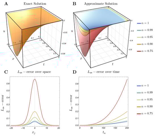
Figure 4. Example 1: (A) Exact solution; (B) approximate solution with $\alpha =1,0.99,0.95,0.9,0.75$ and (C,D) $L_{\infty }$-error over space and time with $\alpha =1,0.99,0.95,0.9,0.75$.

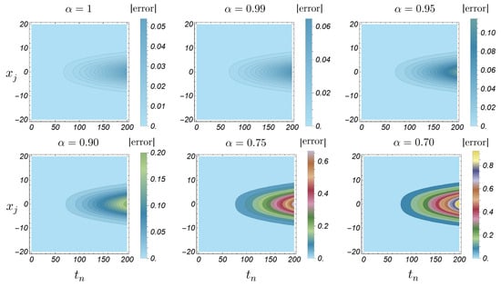
Figure 5. Absolute error heatmap for Example 1 with different values of $\alpha$.

Applying the recurrence relation for the iterative Laplace transform method in Equation (26) leads to

$$\begin{array}{cc}\hfill & \alpha =1.00:u_0(x,t)=t^2(x^2-x)-{\displaystyle \frac{1}{105}}64t^{7/2}-{\displaystyle \frac{2t^3}{3}},u_1(x,t)={\displaystyle \frac{64t^{7/2}}{105}}+{\displaystyle \frac{2t^3}{3}},\hfill \\ \hfill & \alpha =0.99:u_0(x,t)=t^2(x^2-x)-{\displaystyle \frac{4t^{299/100}}{\Gamma \left(\frac{399}{100}\right)}}-{\displaystyle \frac{4\sqrt{\pi }{t}^{349/100}}{\Gamma \left(\frac{449}{100}\right)}},u_1(x,t)={\displaystyle \frac{4t^{299/100}}{\Gamma \left(\frac{399}{100}\right)}}+{\displaystyle \frac{4\sqrt{\pi }{t}^{349/100}}{\Gamma \left(\frac{449}{100}\right)}},\hfill \\ \hfill & \alpha =0.95:u_0(x,t)=t^2(x^2-x)-{\displaystyle \frac{4t^{59/20}}{\Gamma \left(\frac{79}{20}\right)}}-{\displaystyle \frac{4\sqrt{\pi }{t}^{69/20}}{\Gamma \left(\frac{89}{20}\right)}},u_1(x,t)={\displaystyle \frac{4t^{59/20}}{\Gamma \left(\frac{79}{20}\right)}}+{\displaystyle \frac{4\sqrt{\pi }{t}^{69/20}}{\Gamma \left(\frac{89}{20}\right)}},\hfill \\ \hfill & \alpha =0.90:u_0(x,t)=t^2(x^2-x)-{\displaystyle \frac{4t^{29/10}}{\Gamma \left(\frac{39}{10}\right)}}-{\displaystyle \frac{4\sqrt{\pi }{t}^{17/5}}{\Gamma \left(\frac{22}{5}\right)}},u_1(x,t)={\displaystyle \frac{4\sqrt{\pi }{t}^{17/5}}{\Gamma \left(\frac{22}{5}\right)}}+{\displaystyle \frac{4t^{29/10}}{\Gamma \left(\frac{39}{10}\right)}},\hfill \\ \hfill & \alpha =0.75:u_0(x,t)=t^2(x^2-x)-{\displaystyle \frac{4t^{11/4}}{\Gamma \left(\frac{15}{4}\right)}}-{\displaystyle \frac{4\sqrt{\pi }{t}^{13/4}}{\Gamma \left(\frac{17}{4}\right)}},u_1(x,t)={\displaystyle \frac{4t^{11/4}}{\Gamma \left(\frac{15}{4}\right)}}+{\displaystyle \frac{4\sqrt{\pi }{t}^{13/4}}{\Gamma \left(\frac{17}{4}\right)}},\hfill \end{array}$$

and, in all cases, $u_i(x,t)=0$, for all $i\ge 2$. Hence, the approximate solution is

$$u_{\mathrm{app}}^{\mathcal{L}}(x,t)=u_0(x,t)+u_1(x,t)=t^2(x^2-x)=u(x,t).$$

Thus, the approximate solution converges to the exact solution after two iterations. This is because the structure of the function

$$H(x,t)={\displaystyle \frac{2}{\Gamma (3-\alpha )}}x(x-1)t^{2-\alpha }-2t^2-{\displaystyle \frac{4\Gamma (1/2)}{\Gamma (7/2)}}{t}^{{\displaystyle \frac{5}{2}}},$$

which consists only of integer powers of x. As a result, the term $\mathcal{L}\left[{\displaystyle \frac{{\partial }^2{u}_{i-1}(x,t)}{\partial x^2}}\right]$ will disappear after a finite number of derivatives, ensuring the rapid convergence of the approximation.

Example 2. 

Consider the FPIDE with a weakly singular kernel:

$$\begin{array}{cc}\hfill & D_t^{\alpha }u(x,t)=u_{xx}(x,t)+{\int }_0^t{(t-s)}^{\beta -1}{u}_{xx}(x,s)ds\hfill \\ \hfill & +sin\left(\pi x\right)\left({\displaystyle \frac{24}{\Gamma (5-\alpha )}}{t}^{4-\alpha }+{\pi }^2{t}^4+{\displaystyle \frac{24{\pi }^2}{\beta (\beta +1)(\beta +2)(\beta +3)(\beta +4)}}{t}^{\beta +4}\right),\hfill \\ \hfill & \mathit{Boundary}\mathit{conditions}:u(0,t)=u(1,t)=0,\hfill \\ \hfill & \mathit{Initial}\mathit{condition}:u(x,0)=0,\hfill \end{array}$$

(29)

with $\Omega =[0,1]\times [0,1]$. Then, the exact solution is

$$u(x,t)=t^{4}sin\left(\pi x\right).$$

In Figure 6, Figure 7, Figure 8, Figure 9, Figure 10 and Figure 11, we plot the exact and approximate solutions along with $L_{\infty }$-error and absolute error. The same qualitative behavior is observed as in Example 1 when $\alpha$ is decreased. We note that, for $\alpha =1$, the exact solution remains close to the approximate one for values of $\alpha$ near 1. As $\alpha$ decreases further, the solution curve shifts upward, which results in larger error values; see Figure 6, Figure 8 and Figure 10. Furthermore, the absolute error distribution aligns with the shape of the exact solution, reaching its largest values where the solution itself is largest—particularly at $x_j=0.5$, as illustrated in Figure 7, Figure 9 and Figure 11. Additionally, we observe that the error decreases as $\beta$ increases.

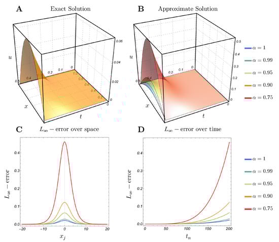
Figure 6. Example 2 with $\beta =0.25$: (A) Exact solution; (B) approximate solution with $\alpha =1,0.99,0.95,0.9,0.75$ and (C,D) $L_{\infty }$-error over space and time with $\alpha =1,0.99,0.95,0.9,0.75$.

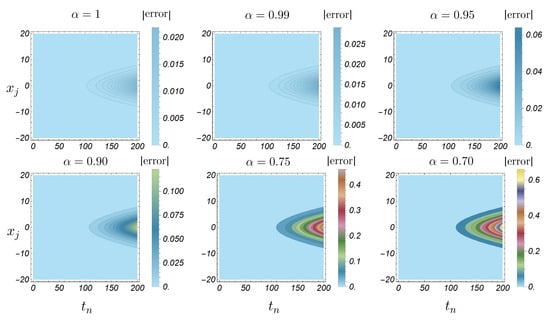
Figure 7. Absolute error heatmap for Example 2 with $\beta =0.25$ and different values of $\alpha$.

Figure 8. Example 2 with $\beta =0.5$: (A) Exact solution; (B) approximate solution with $\alpha =1,0.99,0.95,0.9,0.75$ and (C,D) $L_{\infty }$-error over space and time with $\alpha =1,0.99,0.95,0.9,0.75$.

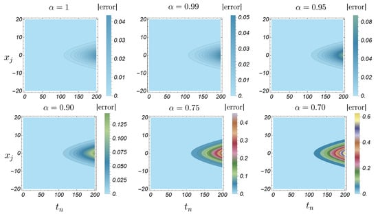
Figure 9. Absolute error heatmap for Example 2 with $\beta =0.5$ and different values of $\alpha$.

Figure 10. Example 2 with $\beta =0.75$: (A) Exact solution; (B) approximate solution with $\alpha =1,0.99,0.95,0.9,0.75$ and (C,D) $L_{\infty }$-error over space and time with $\alpha =1,0.99,0.95,0.9,0.75$.

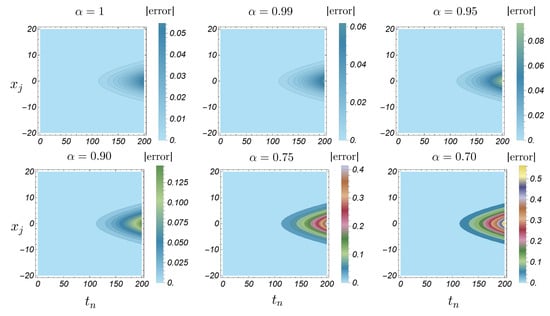
Figure 11. Absolute error heatmap for Example 2 with $\beta =0.75$ and different values of $\alpha$.

For comparison in this example, we apply the recurrence relation for the iterative Laplace transform method in Equation (26) when $\beta =0.5$ and $\alpha =0.99$. Consequently, we have

$$\begin{array}{cc}\hfill & u_0(x,t)=\left({\displaystyle \frac{24{\pi }^2{t}^{499/100}}{\Gamma \left(\frac{599}{100}\right)}}+{\displaystyle \frac{24{\pi }^{5/2}{t}^{549/100}}{\Gamma \left(\frac{649}{100}\right)}}+t^4\right)sin\left(\pi x\right),\hfill \\ \hfill & u_1(x,t)=-24{\pi }^2{t}^{499/100}\left({\displaystyle \frac{{\pi }^2{t}^{99/100}}{\Gamma \left(\frac{349}{50}\right)}}+{\displaystyle \frac{2{\pi }^{5/2}{t}^{149/100}}{\Gamma \left(\frac{187}{25}\right)}}+{\displaystyle \frac{{\pi }^3{t}^{199/100}}{\Gamma \left(\frac{399}{50}\right)}}+{\displaystyle \frac{\sqrt{\pi }\sqrt{t}}{\Gamma \left(\frac{649}{100}\right)}}+{\displaystyle \frac{1}{\Gamma \left(\frac{599}{100}\right)}}\right)sin\left(\pi x\right),\hfill \\ \hfill & u_2(x,t)=24{\pi }^4{t}^{299/50}\left({\displaystyle \frac{{\pi }^2{t}^{99/100}}{\Gamma \left(\frac{797}{100}\right)}}+{\displaystyle \frac{3{\pi }^{5/2}{t}^{149/100}}{\Gamma \left(\frac{847}{100}\right)}}+{\displaystyle \frac{3{\pi }^3{t}^{199/100}}{\Gamma \left(\frac{897}{100}\right)}}+{\displaystyle \frac{{\pi }^{7/2}{t}^{249/100}}{\Gamma \left(\frac{947}{100}\right)}}+{\displaystyle \frac{\pi t}{\Gamma \left(\frac{399}{50}\right)}}\right.\hfill \\ \hfill & \left.+{\displaystyle \frac{2\sqrt{\pi }\sqrt{t}}{\Gamma \left(\frac{187}{25}\right)}}+{\displaystyle \frac{1}{\Gamma \left(\frac{349}{50}\right)}}\right)sin\left(\pi x\right).\hfill \end{array}$$

Hence, the approximate solution is

$$\begin{array}{cc}{u}_{\mathrm{app}}^{\mathcal{L}}(x,t)\hfill & =u_0(x,t)+u_1(x,t)+u_2(x,t)\hfill \\ & =t^4\left({\displaystyle \frac{24{\pi }^6{t}^{297/100}}{\Gamma \left(\frac{797}{100}\right)}}+{\displaystyle \frac{72{\pi }^{13/2}{t}^{347/100}}{\Gamma \left(\frac{847}{100}\right)}}+{\displaystyle \frac{72{\pi }^7{t}^{397/100}}{\Gamma \left(\frac{897}{100}\right)}}+{\displaystyle \frac{24{\pi }^{15/2}{t}^{447/100}}{\Gamma \left(\frac{947}{100}\right)}}+1\right)sin\left(\pi x\right).\hfill \end{array}$$

Table 1 shows that both the $\mathrm{sinc}$-collocation and iterative Laplace transform methods provide good approximations to the exact solution of the FPIDE in Example 2 at $t=0.2$ when $\alpha =0.99$ and $\beta =0.5$. However, the iterative Laplace transform method outperforms the $\mathrm{sinc}$-collocation method in terms of accuracy across all tested $x_j$ points.

Table 1. Error comparison between the $\mathrm{sinc}$-collocation and Iterative Laplace transform methods at different $x_j$ when $t_{80}=0.2$ in Example 2. We take $\alpha =0.99$ and $\beta =0.5$.

j	${\mathit{x}}_{\mathit{j}}$	$\mathbf{sinc}$-Collocation Method Error	Iterative Laplace Method Error
−18	0.0001234	6.77366 $\times {10}^{-8}$	5.35182 $\times {10}^{-8}$
−4	0.119203	2.65155 $\times {10}^{-4}$	5.05002 $\times {10}^{-5}$
−2	0.268941	5.42283 $\times {10}^{-4}$	1.03253 $\times {10}^{-4}$
0	0.5	7.2509 $\times {10}^{-4}$	1.38056 $\times {10}^{-4}$
2	0.731059	5.42283 $\times {10}^{-4}$	1.03253 $\times {10}^{-4}$
4	0.880797	2.65155 $\times {10}^{-4}$	5.05002 $\times {10}^{-5}$
18	0.999877	6.77366 $\times {10}^{-8}$	5.35182 $\times {10}^{-8}$

The temporal errors of the suggested method at the spatial point $x=0.97$ for different time step sizes $\Delta t$ with fixed parameters $\alpha =0.99$, $\beta =0.5$, and spatial resolution $N_x=100$ are shown in Table 2. We can calculate the maximum norm of the error $\parallel u-u_{\mathrm{app}}{\parallel }_{\infty }$ at different time steps. From Table 2, we observe that when the time step size $\Delta t$ is halved, the corresponding error is reduced by approximately a factor of 40. This behavior indicates that the spatial error, which is of exponential order, consequently took center stage, hiding the actual temporal convergence and producing false results.

Table 2. Temporal error in Example 2 at $x=0.97$, with fixed $N_x=100$, $\alpha =0.99$, and $\beta =0.5$.

$\mathbf{\Delta }\mathit{t}$	$\parallel \mathit{u}-{\mathit{u}}_{\mathbf{app}}{\parallel }_{\mathit{\infty }}$
$1/100$	$1.21\times {10}^{-3}$
$1/200$	$3.06\times {10}^{-5}$
$1/400$	$7.66\times {10}^{-7}$
$1/800$	$1.91\times {10}^{-8}$

7. Conclusions

In this article, we have solved a time-fractional partial integro-differential equation (FPIDE) with a weakly singular kernel using the $\mathrm{sinc}$-collocation and iterative Laplace transform methods. The $\mathrm{sinc}$-collocation method has been employed to discretize the spatial domain, while a combination of numerical techniques has been utilized for temporal discretization. Consequently, a symmetric discrete system of equations has been developed. Subsequently, an upper bound on the error was determined, and a convergence analysis was conducted. Since the considered FPIDE has the convolution property, we have applied the iterative Laplace transform method to solve it. For comparison, we have considered two numerical examples. We have observed that the absolute error distribution of the $\mathrm{sinc}$-collocation method exhibits an almost perfect symmetry about the spatial domain’s midpoint due to the discrete system’s symmetrical property. Moreover, we have noted that the approximation solution with various fractional-order $\alpha \in (0,1)$ exhibits the same behavior as the exact solution for which $\alpha =1$. Within the theory of fractional calculus, it is evident that the approximate solution consistently tends to the exact solution of the problem when the fractional derivative $\alpha$ tends to 1, Additionally, the parameter $\beta$, the order of singularity inside the kernel in the FPIDE, has shown effects on the maximum error with different $\alpha$. Numerical experiments have demonstrated that both the $\mathrm{sinc}$-collocation method and the iterative Laplace transform approach yield accurate approximations to the exact solution.

Future research may include fractional integro-differential equations with nonlinear term $N\left(u\right(x,t\left)\right)$ and tempered kernels $K(t,s)=e^{-\lambda (t-s)}{(t-s)}^{\beta -1},\lambda >0,\beta \in (0,1)$, to model systems with fading memory, where past influences decay exponentially over time. Due to its exponential damping, this kernel circumvents the infinite-memory problem of classical fractional models. It is used in applications such as viscoelastic materials, financial models with finite variance, and anomalous diffusion in heterogeneous media. Moreover, we may extend the theoretical analysis to two- and three-dimensional problems, as well as semi-linear formulations.

References

- Sun, T.C.; DarAssi, M.H.; Alfwzan, W.F.; Khan, M.A.; Alqahtani, A.S.; Alshahrani, S.S.; Muhammad, T. Mathematical modeling of COVID-19 with vaccination using fractional derivative: A case study. Fractal Fract. 2023, 7, 234. [Google Scholar] [CrossRef]
- Dababneh, A.; Djenina, N.; Ouannas, A.; Grassi, G.; Batiha, I.M.; Jebril, I.H. A new incommensurate fractional-order discrete COVID-19 model with vaccinated individuals compartment. Fractal Fract. 2022, 6, 456. [Google Scholar] [CrossRef]
- Adolfsson, K.; Enelund, M.; Olsson, P. On the fractional order model of viscoelasticity. Mech. Time-Depend. Mater. 2005, 9, 15–34. [Google Scholar] [CrossRef]
- Tang, X.; Luo, Y.; Han, B. Fractional-order gas film model. Fractal Fract. 2022, 6, 561. [Google Scholar] [CrossRef]
- Li, M.; Chen, L.; Zhou, Y. Sinc Collocation Method to Simulate the Fractional Partial Integro-Differential Equation with a Weakly Singular Kernel. Axioms 2023, 12, 898. [Google Scholar] [CrossRef]
- Fakhari, H.; Mohebbi, A. Galerkin spectral and finite difference methods for the solution of fourth-order time fractional partial integro-differential equation with a weakly singular kernel. J. Appl. Math. Comput. 2024, 70, 5063–5080. [Google Scholar] [CrossRef]
- Mohib, A.; Elbostani, S.; Rachid, A.; El Jid, R. Numerical approximation of a generalized time fractional partial integro-differential equation of Volterra type based on a meshless method. Partial Differ. Equ. Appl. Math. 2024, 11, 100791. [Google Scholar] [CrossRef]
- Panda, A.; Mohapatra, J. Analysis of Some Semi-analytical Methods for the Solutions of a Class of Time Fractional Partial Integro-differential Equations. Int. J. Appl. Comput. Math 2024, 10, 54. [Google Scholar] [CrossRef]
- Darweesh, A.; Alquran, M.; Aghzawi, K. New numerical treatment for a family of two-dimensional fractional Fredholm integro-differential equations. Algorithms 2020, 13, 1–37. [Google Scholar] [CrossRef]
- Dhunde, R. Double Laplace Transform Method for Solving Fractional Fourth-Order Partial Integro-Differential Equations with Weakly Singular Kernel. Indian J. Sci. Technol. 2024, 17, 3712–3718. [Google Scholar] [CrossRef]
- Gu, X.M.; Wu, S.L. A parallel-in-time iterative algorithm for Volterra partial integro-differential problems with weakly singular kernel. J. Comput. Phys. 2020, 417, 109576. [Google Scholar] [CrossRef]
- Zhao, Y.L.; Gu, X.M.; Ostermann, A. A preconditioning technique for an all-at-once system from Volterra subdiffusion equations with graded time steps. J. Sci. Comput. 2021, 88, 11. [Google Scholar] [CrossRef]
- Luo, Z.; Zhang, X.; Wei, L. Analysis of a High-Accuracy Numerical Method for Time-Fractional Integro-Differential Equations. Fractal Fract. 2023, 7, 480. [Google Scholar] [CrossRef]
- Qiu, W.; Xu, D.; Guo, J. The Crank-Nicolson-type Sinc-Galerkin method for the fourth-order partial integro-differential equation with a weakly singular kernel. Appl. Numer. Math. 2021, 159, 239–258. [Google Scholar] [CrossRef]
- Miller, K.S.; Ross, B. An Introduction to the Fractional Calculus and Fractional Differential Equations; Wiley-Interscience: Hoboken, NJ, USA, 1993. [Google Scholar]
- Kubica, A.; Ryszewska, K.; Yamamoto, M. Time-Fractional Differential Equations: A Theoretical Introduction; Springer: Berlin/Heidelberg, Germany, 2020. [Google Scholar]
- Wang, Y.; Yan, Y.; Yan, Y.; Pani, A.K. Higher order time stepping methods for subdiffusion problems based on weighted and shifted Grünwald–Letnikov formulae with nonsmooth data. J. Sci. Comput. 2020, 83, 40. [Google Scholar] [CrossRef]
- Benson, D.A.; Wheatcraft, S.W.; Meerschaert, M.M. Application of a fractional advection-dispersion equation. Water Resour. Res. 2000, 36, 1403–1412. [Google Scholar] [CrossRef]
- Bagley, R.L.; Torvik, P.J. A theoretical basis for the application of fractional calculus to viscoelasticity. J. Rheol. 1983, 27, 201–210. [Google Scholar] [CrossRef]
- Nigmatullin, R. The realization of the generalized transfer equation in a medium with fractal geometry. Phys. Status Solidi (B) Basic Res. 1986, 133, 425–430. [Google Scholar] [CrossRef]
- Sakamoto, K.; Yamamoto, M. Initial value/boundary value problems for fractional diffusion-wave equations and applications to some inverse problems. J. Math. Anal. Appl. 2011, 382, 426–447. [Google Scholar] [CrossRef]
- Luchko, Y. Initial-boundary-value problems for the generalized multi-term time-fractional diffusion equation. J. Math. Anal. Appl. 2011, 374, 538–548. [Google Scholar] [CrossRef]
- Yang, Y. Jacobi spectral Galerkin methods for Volterra integral equations with weakly singular kernel. Bull. Korean Chem. Soc. 2016, 53, 247–262. [Google Scholar] [CrossRef]
- Lund, J.; Bowers, K.L. Sinc Methods for Quadrature and Differential Equations; SIAM: Philadelphia, PA, USA, 1992. [Google Scholar]
- Stenger, F. Numerical Methods Based on Sinc and Analytic Functions; Springer Science & Business Media: Berlin/Heidelberg, Germany, 1993; Volume 20. [Google Scholar]
- McNamee, J.; Stenger, F.; Whitney, E. Whittaker’s cardinal function in retrospect. Math. Comput. 1971, 25, 141–154. [Google Scholar]
- Gamelin, T. Complex Analysis; Springer Science & Business Media: Berlin/Heidelberg, Germany, 2003. [Google Scholar]
- Meerschaert, M.M.; Tadjeran, C. Finite difference approximations for fractional advection–dispersion flow equations. J. Comput. Appl. Math. 2004, 172, 65–77. [Google Scholar] [CrossRef]
- Tian, W.; Zhou, H.; Deng, W. A class of second order difference approximations for solving space fractional diffusion equations. Math. Comput. 2015, 84, 1703–1727. [Google Scholar] [CrossRef]
- Gao, G.h.; Sun, H.w.; Sun, Z.z. Some high-order difference schemes for the distributed-order differential equations. J. Comput. Phys. 2015, 298, 337–359. [Google Scholar] [CrossRef]
- Linz, P. Analytical and Numerical Methods for Volterra Equations; SIAM: Philadelphia, PA, USA, 1985. [Google Scholar]
- Dixon, J. On the order of the error in discretization methods for weakly singular second kind non-smooth solutions. BIT Numer. Math. 1985, 25, 623–634. [Google Scholar] [CrossRef]
- Fahim, A.; Fariborzi Araghi, M.A.; Rashidinia, J.; Jalalvand, M. Numerical solution of Volterra partial integro-differential equations based on sinc-collocation method. Adv. Differ. Equ. 2017, 2017, 1–21. [Google Scholar] [CrossRef]
- Alghamdi, N.; Ellahi, R.; Asjad, M.; Khan, M.I.; Ali, H.M. ψ-Laplace Transform Adomian Decomposition Method for Solving Fractional Differential Equations with Applications. Mathematics 2024, 12, 3499. [Google Scholar]
- Sharma, S.; Bairwa, R. Iterative Laplace transform method for solving fractional heat and wave-like equations. Res. J. Math. Stat. Sci. 2015, 2320, 6047. [Google Scholar]
- Kilbas, A.A.; Srivastava, H.M.; Trujillo, J.J. Theory and Applications of Fractional Differential Equations; Elsevier: Amsterdam, The Netherlands, 2006; Volume 204. [Google Scholar]
- Al-Khaled, K. Numerical solution of time-fractional partial differential equations using Sumudu decomposition method. Rom. J. Phys. 2015, 60, 99–110. [Google Scholar]
Disclaimer/Publisher’s Note: The statements, opinions and data contained in all publications are solely those of the individual author(s) and contributor(s) and not of MDPI and/or the editor(s). MDPI and/or the editor(s) disclaim responsibility for any injury to people or property resulting from any ideas, methods, instructions or products referred to in the content. |
© 2025 by the authors. Licensee MDPI, Basel, Switzerland. This article is an open access article distributed under the terms and conditions of the Creative Commons Attribution (CC BY) license (https://creativecommons.org/licenses/by/4.0/).