An Averaging Principle for Hilfer Fractional Stochastic Evolution Equations with Non-Instantaneous Impulses

Abstract

This paper investigates non-instantaneous impulsive Hilfer fractional stochastic evolution equations. To obtain a more accurate convergence rate, an equivalent form of the above equation is derived by the time-scale separation method. Then, we prove that the solution of the equivalent equation converges to that of the averaged equation. Furthermore, we estimate the convergence rate between the exact and approximate solutions of the equation. Finally, we provide an example to justify our result.

1. Introduction

This paper concentrates on the fractional stochastic evolution equations as follows

$$\left\{\begin{array}{c}{\mathbb{D}}_{\tau }^{\alpha ,\beta }\zeta \left(\tau \right)=\mathcal{A}\zeta \left(\tau \right)+\mathcal{F}({\displaystyle \frac{\tau }{\epsilon }},\zeta \left(\tau \right))+\mathcal{G}({\displaystyle \frac{\tau }{\epsilon }},\zeta \left(\tau \right)){\displaystyle \frac{dW\left(\tau \right)}{d\tau }}\hfill \\ +\mathcal{H}({\displaystyle \frac{\tau }{\epsilon }},\zeta \left(\tau \right)){\displaystyle \frac{d{B}^H\left(\tau \right)}{d\tau }},\tau \in ({\varsigma }_i,{\tau }_{i+1}],i=0,1,2,\cdots ,n,\hfill \\ \zeta \left(\tau \right)=\epsilon {\Phi }_j(\tau ,\zeta \left(\tau \right)),\tau \in ({\tau }_j,{\varsigma }_j],j=1,2,\cdots ,n,\hfill \\ {\mathbb{I}}_{\tau }^{(1-\alpha )(1-\beta )}\zeta \left(0\right)={\zeta }_0,\hfill \end{array}\right.$$

(1)

where ${\mathbb{D}}_{\tau }^{\alpha ,\beta }$ is the Hilfer derivative of order $0<\alpha <1$ and type $0\le \beta \le 1$, and $\tau \in I=[0,T]$. Let $0<\epsilon \ll 1$ be a small parameter. $\mathbb{H}$ denotes a Hilbert space with the norm ${\parallel ·\parallel }_{\mathbb{H}}$. Let $\mathcal{A}:D\left(\mathcal{A}\right)\to \mathbb{H}$ be the infinitesimal generator of ${\mathcal{C}}_0$-semigroup $\mathcal{T}\left(\tau \right)$. $W\left(\tau \right)$ is an $\mathbb{H}$-valued Wiener process, and $B^H\left(\tau \right)$ is a fractional Brownian motion with $H\in ({\displaystyle \frac{1}{2}},1)$. ${\mathbb{I}}_{\tau }^{(1-\alpha )(1-\beta )}$ indicates the Riemann–Liouville fractional integral. See [1,2,3,4] for more details.

In time intervals without impulses, the nonlinear terms $\mathcal{F}$, $\mathcal{G}$, and $\mathcal{H}$ explicitly depend on the fast-time-scale ${\displaystyle \frac{\tau }{\epsilon }}$. It is difficult to study such highly oscillatory equations directly. Therefore, we give an equivalent slow-time-scale equation for Equation (1) by the time-scale separation method and establish an approximate solution to the equivalent form by the averaging principle.

The advantages of the averaging principle lie in replacing complicated differential equations with simple averaged equations under appropriate conditions and significantly reducing analytical and computational complexity. The stochastic averaging principle originated in Khasminskii’s foundational work [5]. Subsequently, various classes of stochastic differential equations (SDEs) were studied by this principle, including stochastic evolution equations [6,7,8], fractional SDEs [9,10,11,12], and SDEs with fractional Brownian motion [13,14,15,16].

Despite these developments, the averaging principle for non-instantaneous impulsive fractional SDEs remains unresolved. Most existing literature has focused on the qualitative properties of instantaneous impulsive SDEs, such as the uniqueness of solutions [17,18,19,20], the averaging principle [21,22,23], and the exponential stability [24,25]. In contrast, studying non-instantaneous impulsive fractional SDEs has become increasingly important in real-world applications, such as biology, engineering, and medicine. Although Balasubramaniam [26] established the existence of solutions for such equations, exact solutions are generally unavailable due to their non-linearity and memory effects. Consequently, constructing approximate solutions for such equations is necessary.

The key challenges mainly arise from the discontinuity induced by the non-instantaneous impulse term and the rigorous quantification of convergence rates between solutions of the equivalent and averaged equations.

Our main contributions are as follows.

• We derive a novel equivalent form of Equation (1), which can reflect the system’s long-term evolution behavior on a slow time scale and can also more accurately estimate the convergence rate between solutions.
• We show that the equivalent equation’s solution converges to the averaged equation’s solution with an order of convergence $2\alpha -1$, which is related to the fractional order.
• To handle the discontinuity of Equation (1), we partition the entire interval into smaller ones and estimate the convergence between solutions on each small interval.

This paper is organized as follows. In Section 2, the theoretical basis is introduced. In Section 3, the mean square convergence and the order of convergence by the averaging principle are given. Finally, in Section 4, the corresponding numerical simulation results are provided.

2. Preliminaries

Some necessary concepts, as well as lemmas, are given in this section.

Let ${\mathbb{L}}_2(\Omega ,\mathbb{H})$ be the set of all strongly measurable and square-integrable random variables with norm ${\parallel \zeta (·)\parallel }_{{\mathbb{L}}_2}={\left(\mathrm{E}[\parallel \zeta (·,\omega ){\parallel }_{\mathbb{H}}^2]\right)}^{{\displaystyle \frac{1}{2}}}$, where $\omega \in \Omega$, and $\mathrm{E}$ is the expectation.

Assume that $C(I,{\mathbb{L}}_2(\Omega ,\mathbb{H}))$ is the Banach space comprised of all $\mathbb{H}$-valued continuous functions from I to ${\mathbb{L}}_2(\Omega ,\mathbb{H})$ with ${sup}_{\tau \in I}{\mathrm{E}[\parallel \zeta \left(\tau \right)\parallel }_{\mathbb{H}}^2]<\infty$. Let $U_i=({\varsigma }_i,{\tau }_{i+1}],i=0,1,2,\cdots ,n$, and $V_j=({\tau }_j,{\varsigma }_j],j=1,2,\cdots ,n$. The set of all piecewise continuous functions from I to ${\mathbb{L}}_2(\Omega ,\mathbb{H})$ is denoted by

$$\begin{array}{cc}\hfill \mathbf{M}& =P{C}_{(1-\alpha )(1-\beta )}(I,{\mathbb{L}}_2(\Omega ,\mathbb{H}))\hfill \\ \hfill & =\{\zeta :{(\tau -{\varsigma }_i)}^{(1-\alpha )(1-\beta )}\zeta \left(\tau \right)\in C(U_i,{\mathbb{L}}_2(\Omega ,\mathbb{H})),\underset{\tau \to {\varsigma }_i^{+}}{lim}{(\tau -{\varsigma }_i)}^{(1-\alpha )(1-\beta )}\zeta \left(\tau \right)\mathrm{exist},\hfill \\ \hfill & \zeta \left(\tau \right)\in C(V_j,{\mathbb{L}}_2(\Omega ,\mathbb{H})),\underset{\tau \to {\tau }_j^{+}}{lim}\zeta \left(\tau \right)\mathrm{exist}\},\hfill \end{array}$$

and the norm is given by

$$\begin{array}{c}\hfill {\parallel ·\parallel }_{\mathbf{M}}=max\left\{\underset{i=0,1,2,\cdots ,n}{max}\underset{\tau \in U_i}{sup}\parallel {(\tau -{\varsigma }_i)}^{(1-\alpha )(1-\beta )}\zeta \left(\tau \right){\parallel }_{{\mathbb{L}}_2},\underset{j=1,2,\cdots ,n}{max}\underset{\tau \in V_j}{sup}{\parallel \zeta \left(\tau \right)\parallel }_{{\mathbb{L}}_2}\right\}.\end{array}$$

The following lemmas are presented to establish our main result.

Lemma 1

(see [26]). A ${\mathcal{W}}_0$-adopted stochastic process $\zeta \left(\tau \right)$ is a mild solution of Equation (1) if

$$\zeta \left(\tau \right)=\left\{\begin{array}{c}{\mathcal{S}}_{\alpha ,\beta }\left(\tau \right){\zeta }_0+{\int }_0^{\tau }{\mathcal{P}}_{\beta }(\tau -\varsigma )\mathcal{F}({\displaystyle \frac{\varsigma }{\epsilon }},\zeta \left(\varsigma \right))d\varsigma +{\int }_0^{\tau }{\mathcal{P}}_{\beta }(\tau -\varsigma )\mathcal{G}({\displaystyle \frac{\varsigma }{\epsilon }},\zeta \left(\varsigma \right))dW\left(\varsigma \right)\hfill \\ +{\int }_0^{\tau }{\mathcal{P}}_{\beta }(\tau -\varsigma )\mathcal{H}({\displaystyle \frac{\varsigma }{\epsilon }},\zeta \left(\varsigma \right))d{B}^H\left(\varsigma \right),\tau \in [0,{\tau }_1],\hfill \\ \epsilon {\Phi }_j(\tau ,\zeta \left(\tau \right)),\tau \in V_j,j=1,2,\cdots ,n,\hfill \\ {\mathcal{S}}_{\alpha ,\beta }(\tau -{\varsigma }_i){\Phi }_i({\varsigma }_i,\zeta \left({\varsigma }_i\right))+{\int }_{{\varsigma }_i}^{\tau }{\mathcal{P}}_{\beta }(\tau -\varsigma )\mathcal{F}({\displaystyle \frac{\varsigma }{\epsilon }},\zeta \left(\varsigma \right))d\varsigma \hfill \\ +{\int }_{{\varsigma }_i}^{\tau }{\mathcal{P}}_{\beta }(\tau -\varsigma )\mathcal{G}({\displaystyle \frac{\varsigma }{\epsilon }},\zeta \left(\varsigma \right))dW\left(\varsigma \right)\hfill \\ +{\int }_{{\varsigma }_i}^{\tau }{\mathcal{P}}_{\beta }(\tau -\varsigma )\mathcal{H}({\displaystyle \frac{\varsigma }{\epsilon }},\zeta \left(\varsigma \right))d{B}^H\left(\varsigma \right),\tau \in U_i,i=1,2,\cdots ,n,\hfill \end{array}\right.$$

holds, and $n<\infty$, where ${\mathcal{S}}_{\alpha ,\beta }\left(\tau \right)={\mathbb{I}}_{\tau }^{\alpha (1-\beta )}{\mathcal{P}}_{\beta }\left(\tau \right)$, ${\mathcal{P}}_{\beta }\left(\tau \right)={\tau }^{\beta -1}{\int }_0^{\infty }\beta \varsigma {\psi }_{\beta }\left(\varsigma \right)\mathcal{T}\left({\tau }^{\beta }\varsigma \right)d\varsigma$. The wright function ${\psi }_{\beta }\left(\varsigma \right)$ is defined by ${\psi }_{\beta }\left(\varsigma \right)={\sum }_{n=1}^{\infty }{\displaystyle \frac{{(-\varsigma )}^{n-1}}{(n-1)!\Gamma (1-\beta n)}},\varsigma \in [0,\tau ]$.

Lemma 2

(see [2]). For $\tau >0$, if semigroup $\mathcal{T}\left(\tau \right)$ is bounded and continuous, then $\left\{{\mathcal{S}}_{\alpha ,\beta }\left(\tau \right)\right\}$ and $\left\{{\mathcal{P}}_{\beta }\left(\tau \right)\right\}$ are strongly continuous bounded linear operators, and

$$\begin{array}{ccc}\hfill \parallel {\mathcal{S}}_{\alpha ,\beta }\left(\tau \right)\zeta \left(\tau \right)\parallel & \le {\displaystyle \frac{C_T{\tau }^{(1-\alpha )(\beta -1)}}{\Gamma (\alpha +\beta -\alpha \beta )}}\parallel \zeta \left(\tau \right)\parallel ,\parallel {\mathcal{P}}_{\beta }\left(\tau \right)\zeta \left(\tau \right)\parallel \hfill & \hfill \le {\displaystyle \frac{C_T{\tau }^{\beta -1}}{\Gamma \left(\beta \right)}}\parallel \zeta \left(\tau \right)\parallel ,\end{array}$$

where $C_T$ is a constant dependent on T.

The time-scaling characteristic of the Hilfer fractional derivative is presented below.

Lemma 3.

Let the time-scale $\tau =\epsilon \nu$, then

$${\mathbb{D}}_{\nu }^{\alpha ,\beta }f\left(\epsilon \nu \right)={\epsilon }^{\alpha }{\mathbb{D}}_{\tau }^{\alpha ,\beta }f\left(\tau \right).$$

Proof. 

Due to the definition of the Hilfer derivative in [1], we have

$$\begin{array}{cc}\hfill {\mathbb{D}}_{\nu }^{\alpha ,\beta }f\left(\epsilon \nu \right)& ={\displaystyle \frac{1}{{\Gamma }_{\alpha ,\beta }}}{\int }_0^{\nu }{\displaystyle \frac{f\left(\epsilon \varsigma \right)}{{(\nu -\varsigma )}^{\alpha +1}}}d\varsigma \hfill \\ \hfill & ={\displaystyle \frac{{\epsilon }^{\alpha +1}}{{\Gamma }_{\alpha ,\beta }}}{\int }_0^{\epsilon \nu }{\displaystyle \frac{f\left(u\right)}{{(\epsilon \nu -u)}^{\alpha +1}}}{\displaystyle \frac{1}{\epsilon }}du(\mathrm{let}u=\epsilon \varsigma )\hfill \\ \hfill & ={\displaystyle \frac{{\epsilon }^{\alpha }}{{\Gamma }_{\alpha ,\beta }}}{\int }_0^{\tau }{\displaystyle \frac{f\left(u\right)}{{(\tau -u)}^{\alpha +1}}}du(\mathrm{let}\epsilon \nu =\tau )\hfill \\ \hfill & ={\epsilon }^{\alpha }{\mathbb{D}}_{\tau }^{\alpha ,\beta }f\left(\tau \right),\hfill \end{array}$$

where ${\Gamma }_{\alpha ,\beta }=\Gamma (\alpha +(1-\beta ))\Gamma \left((1-\alpha )(1-\beta )\right)$ denotes a generalized Gamma function. □

The equivalent form of Equation (1) is given using the time-scale separation method. Let $\tau =\epsilon \nu$. According to Lemma 3, for any $\tau \in U_i$ with $i=0,1,2,\cdots ,n$, the first equation of Equation (1) can be rewritten as

$${\epsilon }^{-\alpha }{\mathbb{D}}_{\nu }^{\alpha ,\beta }\zeta \left(\epsilon \nu \right)=\mathcal{A}\zeta \left(\epsilon \nu \right)+\mathcal{F}(\nu ,\zeta \left(\epsilon \nu \right))+\mathcal{G}(\nu ,\zeta \left(\epsilon \nu \right)){\displaystyle \frac{dW\left(\epsilon \nu \right)}{\epsilon d\nu }}+\mathcal{H}(\nu ,\zeta \left(\epsilon \nu \right)){\displaystyle \frac{d{B}^H\left(\epsilon \nu \right)}{\epsilon d\nu }}.$$

Let $\zeta \left(\epsilon \nu \right)={\zeta }_{\epsilon }\left(\nu \right)$ and $\nu :=\tau$. Owing to

$$dW\left(\epsilon \nu \right)=\sqrt{\epsilon }dW\left(\nu \right),d{B}^H\left(\epsilon \nu \right)={\epsilon }^{H}d{B}^H\left(\nu \right),$$

the equivalent equation of Equation (1) is as follows

$$\left\{\begin{array}{c}{\mathbb{D}}_{\tau }^{\alpha ,\beta }{\zeta }_{\epsilon }\left(\tau \right)={\epsilon }^{\alpha }\mathcal{A}{\zeta }_{\epsilon }\left(\tau \right)+{\epsilon }^{\alpha }\mathcal{F}(\tau ,{\zeta }_{\epsilon }\left(\tau \right))+{\epsilon }^{\alpha -{\displaystyle \frac{1}{2}}}\mathcal{G}(\tau ,{\zeta }_{\epsilon }\left(\tau \right)){\displaystyle \frac{dW\left(\tau \right)}{d\tau }}\hfill \\ +{\epsilon }^{\alpha +H-1}\mathcal{H}(\tau ,{\zeta }_{\epsilon }\left(\tau \right)){\displaystyle \frac{d{B}^H\left(\tau \right)}{d\tau }},\tau \in U_i,i=0,1,2,\cdots ,n,\hfill \\ {\zeta }_{\epsilon }\left(\tau \right)=\epsilon {\Phi }_j(\tau ,{\zeta }_{\epsilon }\left(\tau \right)),\tau \in V_j,j=1,2,\cdots ,n,\hfill \\ {\mathbb{I}}_{\tau }^{(1-\alpha )(1-\beta )}{\zeta }_{\epsilon }\left(0\right)={\zeta }_0.\hfill \end{array}\right.$$

(2)

By Lemma 1, Equation (2)’s equivalent integral form is given by

$${\zeta }_{\epsilon }\left(\tau \right)=\left\{\begin{array}{c}{\epsilon }^{\alpha }{\mathcal{S}}_{\alpha ,\beta }\left(\tau \right){\zeta }_0+{\epsilon }^{\alpha }{\int }_0^{\tau }{\mathcal{P}}_{\beta }(\tau -\varsigma )\mathcal{F}(\varsigma ,{\zeta }_{\epsilon }\left(\varsigma \right))d\varsigma \hfill \\ +{\epsilon }^{\alpha -{\displaystyle \frac{1}{2}}}{\int }_0^{\tau }{\mathcal{P}}_{\beta }(\tau -\varsigma )\mathcal{G}(\varsigma ,{\zeta }_{\epsilon }\left(\varsigma \right))dW\left(\varsigma \right)\hfill \\ +{\epsilon }^{\alpha +H-1}{\int }_0^{\tau }{\mathcal{P}}_{\beta }(\tau -\varsigma )\mathcal{H}(\varsigma ,{\zeta }_{\epsilon }\left(\varsigma \right))d{B}^H\left(\varsigma \right),\tau \in [0,{\tau }_1],\hfill \\ \epsilon {\Phi }_j(\tau ,{\zeta }_{\epsilon }\left(\tau \right)),\tau \in V_j,j=1,2,\cdots ,n,\hfill \\ {\epsilon }^{\alpha }{\mathcal{S}}_{\alpha ,\beta }(\tau -{\varsigma }_i){\Phi }_i({\varsigma }_i,{\zeta }_{\epsilon }\left({\varsigma }_i\right))+{\epsilon }^{\alpha }{\int }_{{\varsigma }_i}^{\tau }{\mathcal{P}}_{\beta }(\tau -\varsigma )\mathcal{F}(\varsigma ,{\zeta }_{\epsilon }\left(\varsigma \right))d\varsigma \hfill \\ +{\epsilon }^{\alpha -{\displaystyle \frac{1}{2}}}{\int }_{{\varsigma }_i}^{\tau }{\mathcal{P}}_{\beta }(\tau -\varsigma )\mathcal{G}(\varsigma ,{\zeta }_{\epsilon }\left(\varsigma \right))dW\left(\varsigma \right)\hfill \\ +{\epsilon }^{\alpha +H-1}{\int }_{{\varsigma }_i}^{\tau }{\mathcal{P}}_{\beta }(\tau -\varsigma )\mathcal{H}(\varsigma ,{\zeta }_{\epsilon }\left(\varsigma \right))d{B}^H\left(\varsigma \right),\tau \in U_i,i=1,2,\cdots ,n.\hfill \end{array}\right.$$

Remark 1.

In contrast to Equation (1), Equation (2) exhibits a slow time-scale property, which facilitates the investigation of its long-term dynamical behavior and enables a more accurate estimation of the approximate solution.

3. Averaging Principle

This section establishes the mean square convergence between the solution of Equation (2) and its averaged counterpart and determines the convergence order.

Traditionally, the averaging principle typically considers averaging over entire time intervals, making it unsuitable for handling equations with discontinuous right-hand-side functions. Therefore, we impose the following conditions. For notational convenience, the norm in the Hilbert space is denoted by $\parallel ·\parallel$.

$\left(A_1\right)$ Let $\mathcal{F},\mathcal{G},\mathcal{H}:U_i\times \mathbb{H}\to \mathbb{H}$. There exists $L>0$, such that for any ${\zeta }_1,{\zeta }_2\in {\mathbb{L}}_2(\Omega ,\mathbb{H})$ and $\tau \in U_i$, we have

$$\begin{array}{cc}\hfill \parallel \mathsf{\Lambda }(\tau ,{\zeta }_1\left(\tau \right)){\parallel }^2& \le L\left(1+\parallel {\zeta }_1{\left(\tau \right)\parallel }_{{\mathbb{L}}_2}^2\right),\hfill \\ \hfill \parallel \mathsf{\Lambda }(\tau ,{\zeta }_1\left(\tau \right))-\mathsf{\Lambda }(\tau ,{\zeta }_2\left(\tau \right)){\parallel }^2& \le L\parallel {\zeta }_1\left(\tau \right)-{\zeta }_2{\left(\tau \right)\parallel }_{{\mathbb{L}}_2}^2,\hfill \end{array}$$

where $\mathsf{\Lambda }=\mathcal{F},\mathcal{G},\mathcal{H}$;

$\left(A_2\right)$ The functions ${\Phi }_j:V_j\times \mathbb{H}\to \mathbb{H}$ are continuous and there exist positive and nondecreasing functions ${\varrho }_j\left(\tau \right)$ such that

$$\begin{array}{cc}\hfill \parallel {\Phi }_j(\tau ,{\zeta }_1\left(\tau \right)){\parallel }^2& \le {\varrho }_j\left(\tau \right)\left(1+\parallel {\zeta }_1{\left(\tau \right)\parallel }_{{\mathbb{L}}_2}^2\right),\hfill \\ \hfill \parallel {\Phi }_j(\tau ,{\zeta }_1\left(\tau \right))-{\Phi }_j(\tau ,{\zeta }_2\left(\tau \right)){\parallel }^2& \le {\varrho }_j\left(\tau \right)\left(1+\parallel {\zeta }_1\left(\tau \right)-{\zeta }_2{\left(\tau \right)\parallel }_{{\mathbb{L}}_2}^2\right),\hfill \end{array}$$

where $\widehat{\varrho }=max\left\{{\varrho }_j\left(\tau \right),j=1,2,\cdots ,n\right\}$ and $0<\widehat{\varrho }<1$;

$\left(A_3\right)$ For any $\tau \in U_i$, the following estimates hold

$$\begin{array}{cc}\hfill \underset{\tau \in ({\varsigma }_i,{\tau }_{i+1}]}{sup}{\displaystyle \frac{1}{\tau -{\varsigma }_i}}{\int }_{{\varsigma }_i}^{\tau }\parallel \mathcal{F}(\varsigma ,\zeta \left(\varsigma \right))-\overline{\mathcal{F}}\left(\zeta \left(\varsigma \right)\right){\parallel }^{2}d\varsigma & \le {\sigma }_1({\tau }_{i+1}-{\varsigma }_i){\parallel \zeta \left(\tau \right)\parallel }_{{\mathbb{L}}_2}^2,\hfill \\ \hfill \underset{\tau \in ({\varsigma }_i,{\tau }_{i+1}]}{sup}{\displaystyle \frac{1}{\tau -{\varsigma }_i}}{\int }_{{\varsigma }_i}^{\tau }\parallel \mathcal{G}(\varsigma ,\zeta \left(\varsigma \right))-\overline{\mathcal{G}}\left(\zeta \left(\varsigma \right)\right){\parallel }^{2}d\varsigma & \le {\sigma }_2({\tau }_{i+1}-{\varsigma }_i){\parallel \zeta \left(\tau \right)\parallel }_{{\mathbb{L}}_2}^2,\hfill \\ \hfill \underset{\tau \in ({\varsigma }_i,{\tau }_{i+1}]}{sup}{\displaystyle \frac{1}{\tau -{\varsigma }_i}}{\int }_{{\varsigma }_i}^{\tau }\parallel \mathcal{H}(\varsigma ,\zeta \left(\varsigma \right))-\overline{\mathcal{H}}\left(\zeta \left(\varsigma \right)\right){\parallel }^{2}d\varsigma & \le {\sigma }_3({\tau }_{i+1}-{\varsigma }_i){\parallel \zeta \left(\tau \right)\parallel }_{{\mathbb{L}}_2}^2,\hfill \end{array}$$

where ${\sigma }_k(·),k=1,2,3$ are positive bounded functions. Let

$${\sigma }^{\ast }\left(\tau \right)=sup\left\{{\sigma }_k\left(\tau \right),\tau \in ({\varsigma }_i,{\tau }_{i+1}],k=1,2,3,i=0,1,2,\cdots ,n\right\}.$$

We associate Equation (2) with the following averaged form

$$\left\{\begin{array}{c}{\mathbb{D}}_{\tau }^{\alpha ,\beta }{\varphi }_{\epsilon }\left(\tau \right)={\epsilon }^{\alpha }\mathcal{A}{\varphi }_{\epsilon }\left(\tau \right)+{\epsilon }^{\alpha }\overline{\mathcal{F}}\left({\varphi }_{\epsilon }\left(\tau \right)\right)+{\epsilon }^{\alpha -{\displaystyle \frac{1}{2}}}\overline{\mathcal{G}}\left({\varphi }_{\epsilon }\left(\tau \right)\right){\displaystyle \frac{dW\left(\tau \right)}{d\tau }}\hfill \\ +{\epsilon }^{\alpha +H-1}\overline{\mathcal{H}}\left({\varphi }_{\epsilon }\left(\tau \right)\right){\displaystyle \frac{d{B}^H\left(\tau \right)}{d\tau }},\tau \in U_i,i=0,1,2,\cdots ,n,\hfill \\ {\varphi }_{\epsilon }\left(\tau \right)=\epsilon {\Phi }_j(\tau ,{\varphi }_{\epsilon }\left(\tau \right)),\tau \in V_j,j=1,2,\cdots ,n,\hfill \\ {\mathbb{I}}_{\tau }^{(1-\alpha )(1-\beta )}{\varphi }_{\epsilon }\left(0\right)={\zeta }_0,\hfill \end{array}\right.$$

(3)

where the functions $\overline{\mathcal{F}},\overline{\mathcal{G}},\overline{\mathcal{H}}:\mathbb{H}\to \mathbb{H}$ are specified in $\left(A_3\right)$.

By Lemma 1, the equivalent integral form of Equation (2) is as follows

$${\varphi }_{\epsilon }\left(\tau \right)=\left\{\begin{array}{c}{\epsilon }^{\alpha }{\mathcal{S}}_{\alpha ,\beta }\left(\tau \right){\zeta }_0+{\epsilon }^{\alpha }{\int }_0^{\tau }{\mathcal{P}}_{\beta }(\tau -\varsigma )\overline{\mathcal{F}}\left({\varphi }_{\epsilon }\left(\varsigma \right)\right)d\varsigma +{\epsilon }^{\alpha -{\displaystyle \frac{1}{2}}}{\int }_0^{\tau }{\mathcal{P}}_{\beta }(\tau -\varsigma )\overline{\mathcal{G}}\left({\varphi }_{\epsilon }\left(\varsigma \right)\right)dW\left(\varsigma \right)\hfill \\ +{\epsilon }^{\alpha +H-1}{\int }_0^{\tau }{\mathcal{P}}_{\beta }(\tau -\varsigma )\overline{\mathcal{H}}\left({\varphi }_{\epsilon }\left(\varsigma \right)\right)d{B}^H\left(\varsigma \right),\tau \in [0,{\tau }_1],\hfill \\ \epsilon {\Phi }_j(\tau ,{\varphi }_{\epsilon }\left(\tau \right)),\tau \in V_j,j=1,2,\cdots ,n,\hfill \\ {\epsilon }^{\alpha }{\mathcal{S}}_{\alpha ,\beta }(\tau -{\varsigma }_i){\Phi }_i({\varsigma }_i,\varphi \left({\varsigma }_i\right))+{\epsilon }^{\alpha }{\int }_{{\varsigma }_i}^{\tau }{\mathcal{P}}_{\beta }(\tau -\varsigma )\overline{\mathcal{F}}\left({\varphi }_{\epsilon }\left(\varsigma \right)\right)d\varsigma \hfill \\ +{\epsilon }^{\alpha -{\displaystyle \frac{1}{2}}}{\int }_{{\varsigma }_i}^{\tau }{\mathcal{P}}_{\beta }(\tau -\varsigma )\overline{\mathcal{G}}\left({\varphi }_{\epsilon }\left(\varsigma \right)\right)dW\left(\varsigma \right)\hfill \\ +{\epsilon }^{\alpha +H-1}{\int }_{{\varsigma }_i}^{\tau }{\mathcal{P}}_{\beta }(\tau -\varsigma )\overline{\mathcal{H}}\left({\varphi }_{\epsilon }\left(\varsigma \right)\right)d{B}^H\left(\varsigma \right),\tau \in U_i,i=1,2,\cdots ,n,\hfill \end{array}\right.$$

where $n<\infty$. The definitions of ${\mathcal{S}}_{\alpha ,\beta }\left(\tau \right)$ and ${\mathcal{P}}_{\beta }(\tau -\varsigma )$ are the same as Lemma 1.

Lemma 4

( see [26]). Assume that conditions $\left(A_1\right)$–$\left(A_2\right)$ hold, and then Equation (2) has a unique solution ${\zeta }_{\epsilon }\left(\tau \right)$, and $\mathrm{E}\left[\parallel {\zeta }_{\epsilon }{\left(\tau \right)\parallel }^2\right]<\infty$.

Lemma 5.

Assume that conditions $\left(A_1\right)$–$\left(A_3\right)$ hold, Equation (3) admits a unique solution ${\varphi }_{\epsilon }\left(\tau \right)$, and $\mathrm{E}\left[\parallel {\varphi }_{\epsilon }{\left(\tau \right)\parallel }^2\right]<\infty$.

Proof. 

We need to prove $\overline{\mathcal{F}}$, $\overline{\mathcal{G}}$, and $\overline{\mathcal{H}}$ satisfy conditions $\left(A_1\right)$ and $\left(A_2\right)$ as in Equation (2). For $\tau \in U_i$, according to condition $\left(A_3\right)$, we have

$$\begin{array}{cc}\hfill \parallel \overline{\mathcal{F}}\left({\zeta }_1\left(\tau \right)\right){\parallel }^2& \le 2\parallel \overline{\mathcal{F}}\left({\zeta }_1\left(\tau \right)\right)-{\displaystyle \frac{1}{\tau -{\varsigma }_i}}{\int }_{{\varsigma }_i}^{\tau }\mathcal{F}(\varsigma ,{\zeta }_1\left(\varsigma \right))d\varsigma {\parallel }^2+{\displaystyle \frac{2}{\tau -{\varsigma }_i}}\parallel {\int }_{{\varsigma }_i}^{\tau }\mathcal{F}(\varsigma ,{\zeta }_1\left(\varsigma \right))d\varsigma {\parallel }^2\hfill \\ \hfill & \le 2{\sigma }_1(\tau -{\varsigma }_i)\parallel {\zeta }_1\left(\tau \right){\parallel }_{{\mathbb{L}}_2}^2+2L(1+\parallel {\zeta }_1\left(\tau \right){\parallel }_{{\mathbb{L}}_2}^2).\hfill \end{array}$$

$$\begin{array}{cc}\hfill \parallel \overline{\mathcal{F}}\left({\zeta }_1\left(\tau \right)\right)-\overline{\mathcal{F}}\left({\zeta }_2\left(\tau \right)\right){\parallel }^2& \le 3\parallel \overline{\mathcal{F}}\left({\zeta }_1\left(\tau \right)\right)-{\displaystyle \frac{1}{\tau -{\varsigma }_i}}{\int }_{{\varsigma }_i}^{\tau }\mathcal{F}(\varsigma ,{\zeta }_1\left(\varsigma \right))d\varsigma {\parallel }^2\hfill \\ \hfill & +{\displaystyle \frac{3}{\tau -{\varsigma }_i}}\parallel {\int }_{{\varsigma }_i}^{\tau }\left(\mathcal{F}(\varsigma ,{\zeta }_1\left(\varsigma \right))-\mathcal{F}(\varsigma ,{\zeta }_2\left(\varsigma \right))\right)d\varsigma {\parallel }^2\hfill \\ \hfill & +3\parallel {\displaystyle \frac{1}{\tau -{\varsigma }_i}}{\int }_{{\varsigma }_i}^{\tau }\mathcal{F}(\varsigma ,{\zeta }_2\left(\varsigma \right))d\varsigma -\overline{\mathcal{F}}\left({\zeta }_2\left(\tau \right)\right){\parallel }^2\hfill \\ \hfill & \le 3{\sigma }_1(\tau -{\varsigma }_i)\left(\parallel {\zeta }_1{\left(\tau \right)\parallel }_{{\mathbb{L}}_2}^2+{\parallel {\zeta }_2\left(\tau \right)\parallel }_{{\mathbb{L}}_2}^2\right)+3L{\parallel {\zeta }_1\left(\tau \right)-{\zeta }_2\left(\tau \right)\parallel }_{{\mathbb{L}}_2}^2.\hfill \end{array}$$

Since ${\sigma }_1(·)$ is a positive and bounded function, and by Lemma 4, we know $\mathrm{E}\left[\parallel {\zeta }_{\epsilon }{\left(\tau \right)\parallel }^2\right]$ is bounded by a certain positive constant. Therefore, $\overline{\mathcal{F}}$ satisfies condition $\left(A_1\right)$. We can repeat the procedure above to check $\overline{\mathcal{G}}$ and $\overline{\mathcal{H}}$. It is clear that Equation (3) satisfies condition $\left(A_2\right)$. Thus, we complete the proof. □

Now, our main result is presented as follows.

Theorem 1.

Assume that conditions $\left(A_1\right)$–$\left(A_3\right)$ hold. Then, for any given sufficiently small number $\eta >0$, there exists a constant $0<{\epsilon }^{\ast }\ll 1$, such that for any $\epsilon \in (0,{\epsilon }^{\ast }]$ and $\tau \in [0,T]$, we have

$$\parallel {\zeta }_{\epsilon }\left(\tau \right)-{\varphi }_{\epsilon }{\left(\tau \right)\parallel }_{\mathbf{M}}^2\le \eta .$$

Proof. 

To deal with the discontinuity caused by the non-instantaneous impulse term, we divide the whole interval into three parts and consider the convergence on each interval separately.

Part 1. For $\tau \in [0,{\tau }_1]$, due to Equations (2) and (3), we get

$$\begin{array}{cc}\hfill & \mathrm{E}\left[\underset{\tau \in [0,{\tau }_1]}{sup}{\parallel {\zeta }_{\epsilon }\left(\tau \right)-{\varphi }_{\epsilon }\left(\tau \right)\parallel }^2\right]\hfill \\ \hfill & \le 3{\epsilon }^{2\alpha }\mathrm{E}\left[\underset{\tau \in [0,{\tau }_1]}{sup}\parallel {\int }_0^{\tau }{\mathcal{P}}_{\beta }(\tau -\varsigma )\mathcal{F}(\varsigma ,{\zeta }_{\epsilon }\left(\varsigma \right))d\varsigma -{\int }_0^{\tau }{\mathcal{P}}_{\beta }(\tau -\varsigma )\overline{\mathcal{F}}\left({\varphi }_{\epsilon }\left(\varsigma \right)\right)d\varsigma {\parallel }^2\right]\hfill \\ \hfill & +3{\epsilon }^{2\alpha -1}\mathrm{E}\left[\underset{\tau \in [0,{\tau }_1]}{sup}\parallel {\int }_0^{\tau }{\mathcal{P}}_{\beta }(\tau -\varsigma )\mathcal{G}(\varsigma ,{\zeta }_{\epsilon }\left(\varsigma \right))dW\left(\varsigma \right)-{\int }_0^{\tau }{\mathcal{P}}_{\beta }(\tau -\varsigma )\overline{\mathcal{G}}\left({\varphi }_{\epsilon }\left(\varsigma \right)\right)dW\left(\varsigma \right){\parallel }^2\right]\hfill \\ \hfill & +3{\epsilon }^{2\alpha +2H-2}\mathrm{E}[\underset{\tau \in [0,{\tau }_1]}{sup}\parallel {\int }_0^{\tau }{\mathcal{P}}_{\beta }(\tau -\varsigma )\mathcal{H}(\varsigma ,{\zeta }_{\epsilon }\left(\varsigma \right))d{B}^H\left(\varsigma \right)-\hfill \\ \hfill & {\int }_0^{\tau }{\mathcal{P}}_{\beta }(\tau -\varsigma )\overline{\mathcal{H}}\left({\varphi }_{\epsilon }\left(\varsigma \right)\right)d{B}^H\left(\varsigma \right){\parallel }^2]\hfill \\ \hfill & \le 3{\epsilon }^{2\alpha }{I}_1+3{\epsilon }^{2\alpha -1}{I}_2+3{\epsilon }^{2\alpha +2H-2}{I}_3,\hfill \end{array}$$

(4)

where

$$\begin{array}{cc}\hfill I_1& =\mathrm{E}\left[\underset{\tau \in [0,{\tau }_1]}{sup}\parallel {\int }_0^{\tau }{\mathcal{P}}_{\beta }(\tau -\varsigma )\mathcal{F}(\varsigma ,{\zeta }_{\epsilon }\left(\varsigma \right))d\varsigma -{\int }_0^{\tau }{\mathcal{P}}_{\beta }(\tau -\varsigma )\overline{\mathcal{F}}\left({\varphi }_{\epsilon }\left(\varsigma \right)\right)d\varsigma {\parallel }^2\right],\hfill \\ \hfill I_2& =\mathrm{E}\left[\underset{\tau \in [0,{\tau }_1]}{sup}\parallel {\int }_0^{\tau }{\mathcal{P}}_{\beta }(\tau -\varsigma )\mathcal{G}(\varsigma ,{\zeta }_{\epsilon }\left(\varsigma \right))dW\left(\varsigma \right)-{\int }_0^{\tau }{\mathcal{P}}_{\beta }(\tau -\varsigma )\overline{\mathcal{G}}\left({\varphi }_{\epsilon }\left(\varsigma \right)\right)dW\left(\varsigma \right){\parallel }^2\right],\hfill \\ \hfill I_3& =\mathrm{E}\left[\underset{\tau \in [0,{\tau }_1]}{sup}\parallel {\int }_0^{\tau }{\mathcal{P}}_{\beta }(\tau -\varsigma )\mathcal{H}(\varsigma ,{\zeta }_{\epsilon }\left(\varsigma \right))d{B}^H\left(\varsigma \right)-{\int }_0^{\tau }{\mathcal{P}}_{\beta }(\tau -\varsigma )\overline{\mathcal{H}}\left({\varphi }_{\epsilon }\left(\varsigma \right)\right)d{B}^H\left(\varsigma \right){\parallel }^2\right].\hfill \end{array}$$

According to condition $\left(A_3\right)$, we know that there exist monotonically decreasing functions ${\sigma }_k\left(\tau \right)$, $k=1,2,3$, such that for any $\tau \in ({\varsigma }_0,{\tau }_1]$ (here we let ${\varsigma }_0=0$), the following inequality holds

$$\begin{array}{c}\hfill \underset{\tau \in (0,{\tau }_1]}{sup}{\int }_0^{\tau }\parallel \mathsf{\Lambda }(\varsigma ,{\zeta }_{\epsilon }\left(\varsigma \right))-\overline{\mathsf{\Lambda }}\left({\zeta }_{\epsilon }\left(\varsigma \right)\right){\parallel }^{2}d\varsigma \le {\tau }_1{\sigma }_k\left({\tau }_1\right){\parallel {\zeta }_{\epsilon }\left(\tau \right)\parallel }_{{\mathbb{L}}_2}^2,\end{array}$$

(5)

where $\mathsf{\Lambda }=\mathcal{F},\mathcal{G},\mathcal{H}$ correspond to bounded functions ${\sigma }_k\left({\tau }_1\right)$, $k=1,2,3$, respectively.

From Hölder’s inequality, Lemma 2, condition $\left(A_1\right)$ and (5), we have

$$\begin{array}{cc}\hfill I_1& \le \mathrm{E}\left[\underset{\tau \in [0,{\tau }_1]}{sup}\parallel {\int }_0^{\tau }{\mathcal{P}}_{\beta }(\tau -\varsigma )\left(\mathcal{F}(\varsigma ,{\zeta }_{\epsilon }\left(\varsigma \right))-\overline{\mathcal{F}}\left({\varphi }_{\epsilon }\left(\varsigma \right)\right)\right)d\varsigma {\parallel }^2\right]\hfill \\ \hfill & \le \mathrm{E}\left[\underset{\tau \in [0,{\tau }_1]}{sup}{\int }_0^{\tau }{\parallel {\mathcal{P}}_{\beta }(\tau -\varsigma )\parallel }^{2}d\varsigma \times {\int }_0^{\tau }\parallel \mathcal{F}(\varsigma ,{\zeta }_{\epsilon }\left(\varsigma \right))-\overline{\mathcal{F}}\left({\varphi }_{\epsilon }\left(\varsigma \right)\right){\parallel }^{2}d\varsigma \right]\hfill \\ \hfill & \le {\displaystyle \frac{C_T^2}{{\Gamma }^2\left(\beta \right)}}\mathrm{E}\left[\underset{\tau \in [0,{\tau }_1]}{sup}{\int }_0^{\tau }{(\tau -\varsigma )}^{2(\beta -1)}d\varsigma \times {\int }_0^{\tau }\parallel \mathcal{F}(\varsigma ,{\zeta }_{\epsilon }\left(\varsigma \right))-\overline{\mathcal{F}}\left({\varphi }_{\epsilon }\left(\varsigma \right)\right){\parallel }^{2}d\varsigma \right]\hfill \\ \hfill & \le {\displaystyle \frac{2C_T^2{\tau }_1^{2\beta -1}}{{\Gamma }^2\left(\beta \right)(2\beta -1)}}\mathrm{E}\left[\underset{\tau \in [0,{\tau }_1]}{sup}\right({\int }_0^{\tau }{\parallel \mathcal{F}(\varsigma ,{\zeta }_{\epsilon }\left(\varsigma \right))-\mathcal{F}(\varsigma ,{\varphi }_{\epsilon }\left(\varsigma \right))\parallel }^{2}d\varsigma \hfill \\ \hfill & +{\int }_0^{\tau }{\parallel \mathcal{F}(\varsigma ,{\varphi }_{\epsilon }\left(\varsigma \right))-\overline{\mathcal{F}}\left({\varphi }_{\epsilon }\left(\varsigma \right)\right)\parallel }^{2}d\varsigma \left)\right]\hfill \\ \hfill & \le {\displaystyle \frac{2C_T^2{\tau }_1^{2\beta }{\sigma }^{\ast }\left(\tau \right)}{{\Gamma }^2\left(\beta \right)(2\beta -1)}}\mathrm{E}\left[\parallel {\varphi }_{\epsilon }{\left(\tau \right)\parallel }^2\right]+{\displaystyle \frac{2L{C}_T^2{\tau }_1^{2\beta -1}}{{\Gamma }^2\left(\beta \right)(2\beta -1)}}\mathrm{E}\left[\underset{\tau \in [0,{\tau }_1]}{sup}{\int }_0^{\tau }{\parallel {\zeta }_{\epsilon }\left(\varsigma \right)-{\varphi }_{\epsilon }\left(\varsigma \right)\parallel }^{2}d\varsigma \right]\hfill \\ \hfill & \le {\mathcal{I}}_{11}+{\mathcal{I}}_{12}\mathrm{E}\left[\underset{\tau \in [0,{\tau }_1]}{sup}{\int }_0^{\tau }{\parallel {\zeta }_{\epsilon }\left(\varsigma \right)-{\varphi }_{\epsilon }\left(\varsigma \right)\parallel }^{2}d\varsigma \right],\hfill \end{array}$$

(6)

where

$${\mathcal{I}}_{11}={\displaystyle \frac{2C_T^2{\tau }_1^{2\beta }{\sigma }^{\ast }\left(\tau \right)}{{\Gamma }^2\left(\beta \right)(2\beta -1)}}\mathrm{E}\left[\parallel {\varphi }_{\epsilon }{\left(\tau \right)\parallel }^2\right],{\mathcal{I}}_{12}={\displaystyle \frac{2L{C}_T^2{\tau }_1^{2\beta -1}}{{\Gamma }^2\left(\beta \right)(2\beta -1)}}.$$

By Hölder’s inequality, Lemma 2, ([27], Theorem 7.3, p. 40), conditions $\left(A_2\right)$ and $\left(A_3\right)$, we obtain

$$\begin{array}{cc}\hfill I_2& \le \mathrm{E}\left[\underset{\tau \in [0,{\tau }_1]}{sup}\parallel {\int }_0^{\tau }{\mathcal{P}}_{\beta }(\tau -\varsigma )\left(\mathcal{G}(\varsigma ,{\zeta }_{\epsilon }\left(\varsigma \right))-\overline{\mathcal{G}}\left({\varphi }_{\epsilon }\left(\varsigma \right)\right)\right)dW\left(\varsigma \right){\parallel }^2\right]\hfill \\ \hfill & \le C_1\mathrm{E}\left[\underset{\tau \in [0,{\tau }_1]}{sup}{\int }_0^{\tau }{\parallel {\mathcal{P}}_{\beta }(\tau -\varsigma )\parallel }^{2}d\varsigma \times {\int }_0^{\tau }\parallel \mathcal{G}(\varsigma ,{\zeta }_{\epsilon }\left(\varsigma \right))-\overline{\mathcal{G}}\left({\varphi }_{\epsilon }\left(\varsigma \right)\right){\parallel }^{2}d\varsigma \right]\hfill \\ \hfill & \le {\displaystyle \frac{C_1{C}_T^2}{{\Gamma }^2\left(\beta \right)}}\mathrm{E}\left[\underset{\tau \in [0,{\tau }_1]}{sup}{\int }_0^{\tau }{(\tau -\varsigma )}^{2(\beta -1)}d\varsigma \times {\int }_0^{\tau }\parallel \mathcal{G}(\varsigma ,{\zeta }_{\epsilon }\left(\varsigma \right))-\overline{\mathcal{G}}\left({\varphi }_{\epsilon }\left(\varsigma \right)\right){\parallel }^{2}d\varsigma \right]\hfill \\ \hfill & \le {\displaystyle \frac{2C_1{C}_T^2{\tau }_1^{2\beta -1}}{{\Gamma }^2\left(\beta \right)(2\beta -1)}}\mathrm{E}\left[\underset{\tau \in [0,{\tau }_1]}{sup}\right({\int }_0^{\tau }{\parallel \mathcal{G}(\varsigma ,{\zeta }_{\epsilon }\left(\varsigma \right))-\mathcal{G}(\varsigma ,{\varphi }_{\epsilon }\left(\varsigma \right))\parallel }^{2}d\varsigma \hfill \\ \hfill & +{\int }_0^{\tau }{\parallel \mathcal{G}(\varsigma ,{\varphi }_{\epsilon }\left(\varsigma \right))-\overline{\mathcal{G}}\left({\varphi }_{\epsilon }\left(\varsigma \right)\right)\parallel }^{2}d\varsigma \left)\right]\hfill \\ \hfill & \le {\displaystyle \frac{2C_1{C}_T^2{\tau }_1^{2\beta }{\sigma }^{\ast }\left(\tau \right)}{{\Gamma }^2\left(\beta \right)(2\beta -1)}}\mathrm{E}\left[\parallel {\varphi }_{\epsilon }{\left(\tau \right)\parallel }^2\right]+{\displaystyle \frac{2L{C}_1{C}_T^2{\tau }_1^{2\beta -1}}{{\Gamma }^2\left(\beta \right)(2\beta -1)}}\mathrm{E}\left[\underset{\tau \in [0,{\tau }_1]}{sup}{\int }_0^{\tau }{\parallel {\zeta }_{\epsilon }\left(\varsigma \right)-{\varphi }_{\epsilon }\left(\varsigma \right)\parallel }^{2}d\varsigma \right]\hfill \\ \hfill & \le {\mathcal{I}}_{21}+{\mathcal{I}}_{22}\mathrm{E}\left[\underset{\tau \in [0,{\tau }_1]}{sup}{\int }_0^{\tau }{\parallel {\zeta }_{\epsilon }\left(\varsigma \right)-{\varphi }_{\epsilon }\left(\varsigma \right)\parallel }^{2}d\varsigma \right],\hfill \end{array}$$

(7)

where

$${\mathcal{I}}_{21}={\displaystyle \frac{2C_1{C}_T^2{\tau }_1^{2\beta }{\sigma }^{\ast }\left(\tau \right)}{{\Gamma }^2\left(\beta \right)(2\beta -1)}}\mathrm{E}\left[\parallel {\varphi }_{\epsilon }{\left(\tau \right)\parallel }^2\right],{\mathcal{I}}_{22}={\displaystyle \frac{2L{C}_1{C}_T^2{\tau }_1^{2\beta -1}}{{\Gamma }^2\left(\beta \right)(2\beta -1)}}.$$

By Lemma 2, ([26], Lemma 2.1), conditions $\left(A_2\right)$ and $\left(A_3\right)$, we find

$$\begin{array}{cc}\hfill I_3& \le \mathrm{E}\left[\underset{\tau \in [0,{\tau }_1]}{sup}\parallel {\int }_0^{\tau }{\mathcal{P}}_{\beta }(\tau -\varsigma )\left(\mathcal{H}(\varsigma ,{\zeta }_{\epsilon }\left(\varsigma \right))-\overline{\mathcal{H}}\left({\varphi }_{\epsilon }\left(\varsigma \right)\right)\right)d{B}^H\left(\varsigma \right){\parallel }^2\right]\hfill \\ \hfill & \le C_H\mathrm{E}\left[\underset{\tau \in [0,{\tau }_1]}{sup}{\int }_0^{\tau }{\parallel {\mathcal{P}}_{\beta }(\tau -\varsigma )\parallel }^{2}d\varsigma \times {\int }_0^{\tau }\parallel \mathcal{H}(\varsigma ,{\zeta }_{\epsilon }\left(\varsigma \right))-\overline{\mathcal{H}}\left({\varphi }_{\epsilon }\left(\varsigma \right)\right){\parallel }^{2}d\varsigma \right]\hfill \\ \hfill & \le {\displaystyle \frac{C_H{C}_T^2}{{\Gamma }^2\left(\beta \right)}}\mathrm{E}\left[\underset{\tau \in [0,{\tau }_1]}{sup}{\int }_0^{\tau }{(\tau -\varsigma )}^{2(\beta -1)}d\varsigma \times {\int }_0^{\tau }\parallel \mathcal{H}(\varsigma ,{\zeta }_{\epsilon }\left(\varsigma \right))-\overline{\mathcal{H}}\left({\varphi }_{\epsilon }\left(\varsigma \right)\right){\parallel }^{2}d\varsigma \right]\hfill \\ \hfill & \le {\displaystyle \frac{2C_H{C}_T^2{\tau }_1^{2\beta -1}}{{\Gamma }^2\left(\beta \right)(2\beta -1)}}\mathrm{E}\left[\underset{\tau \in [0,{\tau }_1]}{sup}\right({\int }_0^{\tau }{\parallel \mathcal{H}(\varsigma ,{\zeta }_{\epsilon }\left(\varsigma \right))-\mathcal{H}(\varsigma ,{\varphi }_{\epsilon }\left(\varsigma \right))\parallel }^{2}d\varsigma \hfill \\ \hfill & +{\int }_0^{\tau }{\parallel \mathcal{H}(\varsigma ,{\varphi }_{\epsilon }\left(\varsigma \right))-\overline{\mathcal{H}}\left({\varphi }_{\epsilon }\left(\varsigma \right)\right)\parallel }^{2}d\varsigma \left)\right]\hfill \\ \hfill & \le {\displaystyle \frac{2C_H{C}_T^2{\tau }_1^{2\beta }{\sigma }^{\ast }\left(\tau \right)}{{\Gamma }^2\left(\beta \right)(2\beta -1)}}\mathrm{E}\left[\parallel {\varphi }_{\epsilon }{\left(\tau \right)\parallel }^2\right]+{\displaystyle \frac{2L{C}_H{C}_T^2{\tau }_1^{2\beta -1}}{{\Gamma }^2\left(\beta \right)(2\beta -1)}}\mathrm{E}\left[\underset{\tau \in [0,{\tau }_1]}{sup}{\int }_0^{\tau }{\parallel {\zeta }_{\epsilon }\left(\varsigma \right)-{\varphi }_{\epsilon }\left(\varsigma \right)\parallel }^{2}d\varsigma \right]\hfill \\ \hfill & \le {\mathcal{I}}_{31}+{\mathcal{I}}_{32}\mathrm{E}\left[\underset{\tau \in [0,{\tau }_1]}{sup}{\int }_0^{\tau }{\parallel {\zeta }_{\epsilon }\left(\varsigma \right)-{\varphi }_{\epsilon }\left(\varsigma \right)\parallel }^{2}d\varsigma \right],\hfill \end{array}$$

(8)

where

$${\mathcal{I}}_{31}={\displaystyle \frac{2C_H{C}_T^2{\tau }_1^{2\beta }{\sigma }^{\ast }\left(\tau \right)}{{\Gamma }^2\left(\beta \right)(2\beta -1)}}\mathrm{E}\left[\parallel {\varphi }_{\epsilon }{\left(\tau \right)\parallel }^2\right],{\mathcal{I}}_{32}={\displaystyle \frac{2L{C}_H{C}_T^2{\tau }_1^{2\beta -1}}{{\Gamma }^2\left(\beta \right)(2\beta -1)}}.$$

Plugging (6), (7), and (8) into (4), we obtain the following estimation

$$\begin{array}{cc}\hfill & \mathrm{E}\left[\underset{\tau \in [0,{\tau }_1]}{sup}{\parallel {\zeta }_{\epsilon }\left(\tau \right)-{\varphi }_{\epsilon }\left(\tau \right)\parallel }^2\right]\hfill \\ \hfill & \le 3{\epsilon }^{2\alpha -1}\left(\epsilon {\mathcal{I}}_{11}+{\mathcal{I}}_{21}+{\epsilon }^{2H-1}{\mathcal{I}}_{31}\right)\hfill \\ \hfill & +3{\epsilon }^{2\alpha -1}\left(\epsilon {\mathcal{I}}_{12}+{\mathcal{I}}_{22}+{\epsilon }^{2H-1}{\mathcal{I}}_{32}\right)\mathrm{E}\left[\underset{\tau \in [0,{\tau }_1]}{sup}{\int }_0^{\tau }{\parallel {\zeta }_{\epsilon }\left(\varsigma \right)-{\varphi }_{\epsilon }\left(\varsigma \right)\parallel }^{2}d\varsigma \right]\hfill \\ \hfill & \le P_1(\tau ,\epsilon ){\epsilon }^{2\alpha -1}+P_2(\tau ,\epsilon )\mathrm{E}\left[\underset{\tau \in [0,{\tau }_1]}{sup}{\int }_0^{\tau }{\parallel {\zeta }_{\epsilon }\left(\varsigma \right)-{\varphi }_{\epsilon }\left(\varsigma \right)\parallel }^{2}d\varsigma \right],\hfill \end{array}$$

(9)

where

$$\begin{array}{cc}\hfill P_1(\tau ,\epsilon )& ={\displaystyle \frac{6C_T^2{\tau }_1^{2\beta }{\sigma }^{\ast }\left(\tau \right)}{{\Gamma }^2\left(\beta \right)(2\beta -1)}}\left(\epsilon +C_1+{\epsilon }^{2H-1}{C}_H\right)\mathrm{E}\left[\parallel {\varphi }_{\epsilon }{\left(\tau \right)\parallel }^2\right],\hfill \\ \hfill P_2(\tau ,\epsilon )& ={\displaystyle \frac{6{\epsilon }^{2\alpha -1}L{C}_T^2{\tau }_1^{2\beta -1}}{{\Gamma }^2\left(\beta \right)(2\beta -1)}}\left(\epsilon +C_1+{\epsilon }^{2H-1}{C}_H\right).\hfill \end{array}$$

Applying Gronwall’s inequality, we derive

$$\mathrm{E}\left[\underset{\tau \in [0,{\tau }_1]}{sup}{\parallel {\zeta }_{\epsilon }\left(\tau \right)-{\varphi }_{\epsilon }\left(\tau \right)\parallel }^2\right]\le P_1(\tau ,\epsilon )e^{P_2(\tau ,\epsilon ){\tau }_1}{\epsilon }^{2\alpha -1}.$$

(10)

By choosing appropriate parameters $C_1,C_T,C_H,L$, and $\beta$, there exists $K_1>0$, such that for any $\tau \in [0,{\tau }_1]$, $P_1(\tau ,\epsilon )e^{P_2(\tau ,\epsilon ){\tau }_1}\le K_1$. Thus, inequality (10) is equivalent to

$$\mathrm{E}\left[\underset{\tau \in [0,{\tau }_1]}{sup}{\parallel {\zeta }_{\epsilon }\left(\tau \right)-{\varphi }_{\epsilon }\left(\tau \right)\parallel }^2\right]\le K_1{\epsilon }^{2\alpha -1}.$$

(11)

Consequently, for any given number $\eta >0$, we can select ${\epsilon }_1\left(\eta \right)={\left({\displaystyle \frac{\eta }{K_1}}\right)}^{{\displaystyle \frac{1}{2\alpha -1}}}$ to obtain

$$\underset{\tau \in [0,{\tau }_1]}{sup}{\parallel {\zeta }_{\epsilon }\left(\tau \right)-{\varphi }_{\epsilon }\left(\tau \right)\parallel }_{{\mathbb{L}}_2}^2=\mathrm{E}\left[\underset{\tau \in [0,{\tau }_1]}{sup}{\parallel {\zeta }_{\epsilon }\left(\tau \right)-{\varphi }_{\epsilon }\left(\tau \right)\parallel }^2\right]\le \eta ,$$

where $\epsilon \in (0,{\epsilon }_1\left(\eta \right)]$.

Part 2. For $\tau \in V_j$ with $j=1,2,\cdots ,n$, due to Equations (2) and (3), and condition $\left(A_2\right)$, we obtain

$$\begin{array}{cc}\hfill \mathrm{E}\left[\underset{\tau \in ({\tau }_j,{\varsigma }_j]}{sup}{\parallel {\zeta }_{\epsilon }\left(\tau \right)-{\varphi }_{\epsilon }\left(\tau \right)\parallel }^2\right]& \le {\epsilon }^2\mathrm{E}\left[\underset{\tau \in ({\tau }_j,{\varsigma }_j]}{sup}{\parallel {\Phi }_j(\tau ,{\zeta }_{\epsilon }\left(\tau \right))-{\Phi }_j(\tau ,{\varphi }_{\epsilon }\left(\tau \right))\parallel }^2\right]\hfill \\ \hfill & \le {\epsilon }^2\widehat{\varrho }\mathrm{E}\left[\underset{\tau \in ({\tau }_j,{\varsigma }_j]}{sup}\left(1+\parallel {\zeta }_{\epsilon }\left(\tau \right)-{\varphi }_{\epsilon }{\left(\tau \right)\parallel }^2\right)\right],\hfill \end{array}$$

which is euqivalent to

$$\begin{array}{c}\hfill \mathrm{E}\left[\underset{\tau \in ({\tau }_j,{\varsigma }_j]}{sup}{\parallel {\zeta }_{\epsilon }\left(\tau \right)-{\varphi }_{\epsilon }\left(\tau \right)\parallel }^2\right]\le {\displaystyle \frac{{\epsilon }^2\widehat{\varrho }}{1-{\epsilon }^2\widehat{\varrho }}}.\end{array}$$

(12)

Based on the above analysis, for any given number $\eta >0$, we can select ${\epsilon }_2\left(\eta \right)={({\displaystyle \frac{\eta }{(1+\eta )\widehat{\varrho }}})}^{{\displaystyle \frac{1}{2}}}$ to obtain

$$\underset{\tau \in ({\tau }_j,{\varsigma }_j]}{sup}{\parallel {\zeta }_{\epsilon }\left(\tau \right)-{\varphi }_{\epsilon }\left(\tau \right)\parallel }_{{\mathbb{L}}_2}^2=\mathrm{E}\left[\underset{\tau \in ({\tau }_j,{\varsigma }_j]}{sup}{\parallel {\zeta }_{\epsilon }\left(\tau \right)-{\varphi }_{\epsilon }\left(\tau \right)\parallel }^2\right]\le \eta ,$$

where $\epsilon \in (0,{\epsilon }_2\left(\eta \right)]$.

Part 3. Considering $\tau \in U_i$ with $i=1,2,\cdots ,n$, from Equations (2) and (3), we obtain

$$\begin{array}{cc}\hfill & \mathrm{E}\left[\underset{\tau \in ({\varsigma }_i,{\tau }_{i+1}]}{sup}{\parallel {\zeta }_{\epsilon }\left(\tau \right)-{\varphi }_{\epsilon }\left(\tau \right)\parallel }^2\right]\hfill \\ \hfill & \le 4{\epsilon }^{2\alpha }\mathrm{E}\left[\underset{\tau \in ({\varsigma }_i,{\tau }_{i+1}]}{sup}\parallel {\mathcal{S}}_{\alpha ,\beta }(\tau -{\varsigma }_i){\Phi }_i({\varsigma }_i,{\zeta }_{\epsilon }\left({\varsigma }_i\right))-{\mathcal{S}}_{\alpha ,\beta }(\tau -{\varsigma }_i){\Phi }_i({\varsigma }_i,{\varphi }_{\epsilon }\left({\varsigma }_i\right)){\parallel }^2\right]\hfill \\ \hfill & +4{\epsilon }^{2\alpha }\mathrm{E}\left[\underset{\tau \in ({\varsigma }_i,{\tau }_{i+1}]}{sup}\parallel {\int }_{{\varsigma }_i}^{\tau }{\mathcal{P}}_{\beta }(\tau -\varsigma )\mathcal{F}(\varsigma ,{\zeta }_{\epsilon }\left(\varsigma \right))d\varsigma -{\int }_{{\varsigma }_i}^{\tau }{\mathcal{P}}_{\beta }(\tau -\varsigma )\overline{\mathcal{F}}\left({\varphi }_{\epsilon }\left(\varsigma \right)\right)d\varsigma {\parallel }^2\right]\hfill \\ \hfill & +4{\epsilon }^{2\alpha -1}\mathrm{E}[\underset{\tau \in ({\varsigma }_i,{\tau }_{i+1}]}{sup}\parallel {\int }_{{\varsigma }_i}^{\tau }{\mathcal{P}}_{\beta }(\tau -\varsigma )\mathcal{G}(\varsigma ,{\zeta }_{\epsilon }\left(\varsigma \right))dW\left(\varsigma \right)\hfill \\ \hfill & -{\int }_{{\varsigma }_i}^{\tau }{\mathcal{P}}_{\beta }(\tau -\varsigma )\overline{\mathcal{G}}\left({\varphi }_{\epsilon }\left(\varsigma \right)\right)dW\left(\varsigma \right){\parallel }^2]\hfill \\ \hfill & +4{\epsilon }^{2\alpha +2H-2}\mathrm{E}[\underset{\tau \in ({\varsigma }_i,{\tau }_{i+1}]}{sup}\parallel {\int }_{{\varsigma }_i}^{\tau }{\mathcal{P}}_{\beta }(\tau -\varsigma )\mathcal{H}(\varsigma ,{\zeta }_{\epsilon }\left(\varsigma \right))d{B}^H\left(\varsigma \right)\hfill \\ \hfill & -{\int }_{{\varsigma }_i}^{\tau }{\mathcal{P}}_{\beta }(\tau -\varsigma )\overline{\mathcal{H}}\left({\varphi }_{\epsilon }\left(\varsigma \right)\right)d{B}^H\left(\varsigma \right){\parallel }^2]\hfill \\ \hfill & \le 4{\epsilon }^{2\alpha }{J}_1+4{\epsilon }^{2\alpha }{J}_2+4{\epsilon }^{2\alpha -1}{J}_3+4{\epsilon }^{2\alpha +2H-2}{J}_4,\hfill \end{array}$$

(13)

where

$$\begin{array}{cc}\hfill J_1& =\mathrm{E}\left[\underset{\tau \in ({\varsigma }_i,{\tau }_{i+1}]}{sup}\parallel {\mathcal{S}}_{\alpha ,\beta }(\tau -{\varsigma }_i){\Phi }_i({\varsigma }_i,{\zeta }_{\epsilon }\left({\varsigma }_i\right))-{\mathcal{S}}_{\alpha ,\beta }(\tau -{\varsigma }_i){\Phi }_i({\varsigma }_i,{\varphi }_{\epsilon }\left({\varsigma }_i\right)){\parallel }^2\right],\hfill \\ \hfill J_2& =\mathrm{E}\left[\underset{\tau \in ({\varsigma }_i,{\tau }_{i+1}]}{sup}\parallel {\int }_{{\varsigma }_i}^{\tau }{\mathcal{P}}_{\beta }(\tau -\varsigma )\mathcal{F}(\varsigma ,{\zeta }_{\epsilon }\left(\varsigma \right))d\varsigma -{\int }_{{\varsigma }_i}^{\tau }{\mathcal{P}}_{\beta }(\tau -\varsigma )\overline{\mathcal{F}}\left({\varphi }_{\epsilon }\left(\varsigma \right)\right)d\varsigma {\parallel }^2\right],\hfill \\ \hfill J_3& =\mathrm{E}\left[\underset{\tau \in ({\varsigma }_i,{\tau }_{i+1}]}{sup}\parallel {\int }_{{\varsigma }_i}^{\tau }{\mathcal{P}}_{\beta }(\tau -\varsigma )\mathcal{G}(\varsigma ,{\zeta }_{\epsilon }\left(\varsigma \right))dW\left(\varsigma \right)-{\int }_{{\varsigma }_i}^{\tau }{\mathcal{P}}_{\beta }(\tau -\varsigma )\overline{\mathcal{G}}\left({\varphi }_{\epsilon }\left(\varsigma \right)\right)dW\left(\varsigma \right){\parallel }^2\right],\hfill \\ \hfill J_4& =\mathrm{E}\left[\underset{\tau \in ({\varsigma }_i,{\tau }_{i+1}]}{sup}\parallel {\int }_{{\varsigma }_i}^{\tau }{\mathcal{P}}_{\beta }(\tau -\varsigma )\mathcal{H}(\varsigma ,{\zeta }_{\epsilon }\left(\varsigma \right))d{B}^H\left(\varsigma \right)-{\int }_{{\varsigma }_i}^{\tau }{\mathcal{P}}_{\beta }(\tau -\varsigma )\overline{\mathcal{H}}\left({\varphi }_{\epsilon }\left(\varsigma \right)\right)d{B}^H\left(\varsigma \right){\parallel }^2\right].\hfill \end{array}$$

For $J_1$, using Lemma 2 and condition $\left(A_2\right)$, we have

$$\begin{array}{cc}\hfill J_1& \le \mathrm{E}\left[\underset{\tau \in ({\varsigma }_i,{\tau }_{i+1}]}{sup}\parallel {\mathcal{S}}_{\alpha ,\beta }(\tau -{\varsigma }_i)\left({\Phi }_i({\varsigma }_i,{\zeta }_{\epsilon }\left({\varsigma }_i\right))-{\Phi }_i({\varsigma }_i,{\varphi }_{\epsilon }\left({\varsigma }_i\right))\right){\parallel }^2\right]\hfill \\ \hfill & \le \mathrm{E}\left[\underset{\tau \in ({\varsigma }_i,{\tau }_{i+1}]}{sup}{\displaystyle \frac{C_T^2{(\tau -{\varsigma }_i)}^{2(1-\alpha )(\beta -1)}}{{\Gamma }^2(\alpha +\beta -\alpha \beta )}}\parallel {\Phi }_i({\varsigma }_i,{\zeta }_{\epsilon }\left({\varsigma }_i\right))-{\Phi }_i({\varsigma }_i,{\varphi }_{\epsilon }\left({\varsigma }_i\right)){\parallel }^2\right]\hfill \\ \hfill & \le {\displaystyle \frac{C_T^2{({\tau }_{i+1}-{\varsigma }_i)}^{2(1-\alpha )(\beta -1)}}{{\Gamma }^2(\alpha +\beta -\alpha \beta )}}\mathrm{E}\left[\underset{\tau \in ({\varsigma }_i,{\tau }_{i+1}]}{sup}{\varrho }_i\left(\tau \right)\parallel {\zeta }_{\epsilon }\left(\tau \right)-{\varphi }_{\epsilon }\left(\tau \right){\parallel }^2\right]\hfill \\ \hfill & \le {\displaystyle \frac{\widehat{\varrho }{C}_T^2{\delta }^{2(1-\alpha )(\beta -1)}}{{\Gamma }^2(\alpha +\beta -\alpha \beta )}}\mathrm{E}\left[\underset{\tau \in ({\varsigma }_i,{\tau }_{i+1}]}{sup}\parallel {\zeta }_{\epsilon }\left(\tau \right)-{\varphi }_{\epsilon }\left(\tau \right){\parallel }^2\right],\hfill \end{array}$$

(14)

where $\delta =max\{{\tau }_{i+1}-{\varsigma }_i|i=1,2,\cdots ,n\}$.

Analogous to $I_1$, we estimate $J_2$ as follows

$$\begin{array}{cc}\hfill J_2& \le \mathrm{E}\left[\underset{\tau \in ({\varsigma }_i,{\tau }_{i+1}]}{sup}\parallel {\int }_{{\varsigma }_i}^{\tau }{\mathcal{P}}_{\beta }(\tau -\varsigma )\left(\mathcal{F}(\varsigma ,{\zeta }_{\epsilon }\left(\varsigma \right))-\overline{\mathcal{F}}\left({\varphi }_{\epsilon }\left(\varsigma \right)\right)\right)d\varsigma {\parallel }^2\right]\hfill \\ \hfill & \le \mathrm{E}\left[\underset{\tau \in ({\varsigma }_i,{\tau }_{i+1}]}{sup}{\int }_{{\varsigma }_i}^{\tau }{\parallel {\mathcal{P}}_{\beta }(\tau -\varsigma )\parallel }^{2}d\varsigma \times {\int }_{{\varsigma }_i}^{\tau }\parallel \mathcal{F}(\varsigma ,{\zeta }_{\epsilon }\left(\varsigma \right))-\overline{\mathcal{F}}\left({\varphi }_{\epsilon }\left(\varsigma \right)\right){\parallel }^{2}d\varsigma \right]\hfill \\ \hfill & \le {\displaystyle \frac{2C_T^2}{{\Gamma }^2\left(\beta \right)}}\mathrm{E}[\underset{\tau \in ({\varsigma }_i,{\tau }_{i+1}]}{sup}{\int }_{{\varsigma }_i}^{\tau }{(\tau -\varsigma )}^{2(\beta -1)}d\varsigma \times \hfill \\ \hfill & \left({\int }_{{\varsigma }_i}^{\tau }\parallel \mathcal{F}(\varsigma ,{\zeta }_{\epsilon }\left(\varsigma \right))-\mathcal{F}(\varsigma ,{\varphi }_{\epsilon }\left(\varsigma \right)){\parallel }^{2}d\varsigma +{\int }_{{\varsigma }_i}^{\tau }{\parallel \mathcal{F}(\varsigma ,{\varphi }_{\epsilon }\left(\varsigma \right))-\overline{\mathcal{F}}\left({\varphi }_{\epsilon }\left(\varsigma \right)\right)\parallel }^{2}d\varsigma \right)]\hfill \\ \hfill & \le {\displaystyle \frac{2{\tau }_{i+1}{C}_T^2{\delta }^{2\beta -1}{\sigma }^{\ast }\left(\tau \right)}{{\Gamma }^2\left(\beta \right)(2\beta -1)}}\mathrm{E}\left[\parallel {\varphi }_{\epsilon }{\left(\tau \right)\parallel }^2\right]\hfill \\ \hfill & +{\displaystyle \frac{2L{C}_T^2{\delta }^{2\beta -1}}{{\Gamma }^2\left(\beta \right)(2\beta -1)}}\mathrm{E}\left[\underset{\tau \in ({\varsigma }_i,{\tau }_{i+1}]}{sup}{\int }_{{\varsigma }_i}^{\tau }{\parallel {\zeta }_{\epsilon }\left(\varsigma \right)-{\varphi }_{\epsilon }\left(\varsigma \right)\parallel }^{2}d\varsigma \right].\hfill \end{array}$$

(15)

Similar to the estimations in (7) and (8), we have

$$\begin{array}{cc}\hfill J_3& \le {\displaystyle \frac{2{\tau }_{i+1}{C}_1{C}_T^2{\delta }^{2\beta -1}{\sigma }^{\ast }\left(\tau \right)}{{\Gamma }^2\left(\beta \right)(2\beta -1)}}\mathrm{E}\left[\parallel {\varphi }_{\epsilon }{\left(\tau \right)\parallel }^2\right]\hfill \\ \hfill & +{\displaystyle \frac{2L{C}_1{C}_T^2{\delta }^{2\beta -1}}{{\Gamma }^2\left(\beta \right)(2\beta -1)}}\mathrm{E}\left[\underset{\tau \in ({\varsigma }_i,{\tau }_{i+1}]}{sup}{\int }_{{\varsigma }_i}^{\tau }{\parallel {\zeta }_{\epsilon }\left(\varsigma \right)-{\varphi }_{\epsilon }\left(\varsigma \right)\parallel }^{2}d\varsigma \right],\hfill \end{array}$$

(16)

and

$$\begin{array}{cc}\hfill J_4& \le {\displaystyle \frac{2{\tau }_{i+1}{C}_H{C}_T^2{\delta }^{2\beta -1}{\sigma }^{\ast }\left(\tau \right)}{{\Gamma }^2\left(\beta \right)(2\beta -1)}}\mathrm{E}\left[\parallel {\varphi }_{\epsilon }{\left(\tau \right)\parallel }^2\right]\hfill \\ \hfill & +{\displaystyle \frac{2L{C}_H{C}_T^2{\delta }^{2\beta -1}}{{\Gamma }^2\left(\beta \right)(2\beta -1)}}\mathrm{E}\left[\underset{\tau \in ({\varsigma }_i,{\tau }_{i+1}]}{sup}{\int }_{{\varsigma }_i}^{\tau }{\parallel {\zeta }_{\epsilon }\left(\varsigma \right)-{\varphi }_{\epsilon }\left(\varsigma \right)\parallel }^{2}d\varsigma \right].\hfill \end{array}$$

(17)

By substituting (14)–(17) into (13), we have

$$\begin{array}{cc}\hfill & \left(1-{\displaystyle \frac{4{\epsilon }^{2\alpha }\widehat{\varrho }{C}_T^2{\delta }^{2(1-\alpha )(\beta -1)}}{{\Gamma }^2(\alpha +\beta -\alpha \beta )}}\right)\mathrm{E}\left[\underset{\tau \in ({\varsigma }_i,{\tau }_{i+1}]}{sup}{\parallel {\zeta }_{\epsilon }\left(\tau \right)-{\varphi }_{\epsilon }\left(\tau \right)\parallel }^2\right]\hfill \\ \hfill & \le {\displaystyle \frac{8{\epsilon }^{2\alpha -1}{\tau }_{i+1}{C}_T^2{\delta }^{2\beta -1}{\sigma }^{\ast }\left(\tau \right)}{{\Gamma }^2\left(\beta \right)(2\beta -1)}}\left(\epsilon +C_1+{\epsilon }^{2H-1}{C}_H\right)\mathrm{E}\left[\parallel {\varphi }_{\epsilon }{\left(\tau \right)\parallel }^2\right]\hfill \\ \hfill & +{\displaystyle \frac{8{\epsilon }^{2\alpha -1}L{C}_T^2{\delta }^{2\beta -1}}{{\Gamma }^2\left(\beta \right)(2\beta -1)}}\left(\epsilon +C_1+{\epsilon }^{2H-1}{C}_H\right)\mathrm{E}\left[\underset{\tau \in ({\varsigma }_i,{\tau }_{i+1}]}{sup}{\int }_{{\varsigma }_i}^{\tau }{\parallel {\zeta }_{\epsilon }\left(\varsigma \right)-{\varphi }_{\epsilon }\left(\varsigma \right)\parallel }^{2}d\varsigma \right].\hfill \end{array}$$

This implies

$$\begin{array}{cc}\hfill & \mathrm{E}\left[\underset{\tau \in ({\varsigma }_i,{\tau }_{i+1}]}{sup}{\parallel {\zeta }_{\epsilon }\left(\tau \right)-{\varphi }_{\epsilon }\left(\tau \right)\parallel }^2\right]\hfill \\ \hfill & \le {\displaystyle \frac{{\Gamma }^2(\alpha +\beta -\alpha \beta )\left(\epsilon +C_1+{\epsilon }^{2H-1}{C}_H\right)}{{\Gamma }^2(\alpha +\beta -\alpha \beta )-4{\epsilon }^{2\alpha }\widehat{\varrho }{C}_T^2{\delta }^{2(1-\alpha )(\beta -1)}}}\times {\displaystyle \frac{8{\epsilon }^{2\alpha -1}{C}_T^2{\delta }^{2\beta -1}}{{\Gamma }^2\left(\beta \right)(2\beta -1)}}\times \hfill \\ \hfill & \left({\tau }_{i+1}{\sigma }^{\ast }\left(\tau \right)\mathrm{E}\left[\parallel {\varphi }_{\epsilon }{\left(\tau \right)\parallel }^2\right]+L\mathrm{E}\left[\underset{\tau \in ({\varsigma }_i,{\tau }_{i+1}]}{sup}{\int }_{{\varsigma }_i}^{\tau }{\parallel {\zeta }_{\epsilon }\left(\varsigma \right)-{\varphi }_{\epsilon }\left(\varsigma \right)\parallel }^{2}d\varsigma \right]\right)\hfill \\ \hfill & \le P_3(\tau ,\epsilon ){\epsilon }^{2\alpha -1}+P_4(\tau ,\epsilon )\mathrm{E}\left[\underset{\tau \in ({\varsigma }_i,{\tau }_{i+1}]}{sup}{\int }_{{\varsigma }_i}^{\tau }{\parallel {\zeta }_{\epsilon }\left(\varsigma \right)-{\varphi }_{\epsilon }\left(\varsigma \right)\parallel }^{2}d\varsigma \right],\hfill \end{array}$$

(18)

where

$$\begin{array}{cc}\hfill P_3(\tau ,\epsilon )& ={\Gamma }_{\alpha ,\beta ,T}\times 8{\tau }_{i+1}{C}_T^2{\delta }^{2\beta -1}{\sigma }^{\ast }\left(\tau \right)\left(\epsilon +C_1+{\epsilon }^{2H-1}{C}_H\right)\mathrm{E}\left[\parallel {\varphi }_{\epsilon }{\left(\tau \right)\parallel }^2\right],\hfill \\ \hfill P_4(\tau ,\epsilon )& ={\Gamma }_{\alpha ,\beta ,T}\times 8{\epsilon }^{2\alpha -1}L{C}_T^2{\delta }^{2\beta -1}\left(\epsilon +C_1+{\epsilon }^{2H-1}{C}_H\right),\hfill \\ \hfill {\Gamma }_{\alpha ,\beta ,T}& ={\displaystyle \frac{{\Gamma }^2(\alpha +\beta -\alpha \beta )}{\left({\Gamma }^2(\alpha +\beta -\alpha \beta )-4{\epsilon }^{2\alpha }\widehat{\varrho }{C}_T^2{\delta }^{2(1-\alpha )(\beta -1)}\right){\Gamma }^2\left(\beta \right)(2\beta -1)}}.\hfill \end{array}$$

Applying Gronwall’s inequality, we derive

$$\mathrm{E}\left[\underset{\tau \in ({\varsigma }_i,{\tau }_{i+1}]}{sup}{\parallel {\zeta }_{\epsilon }\left(\tau \right)-{\varphi }_{\epsilon }\left(\tau \right)\parallel }^2\right]\le P_3(\tau ,\epsilon )e^{P_4(\tau ,\epsilon ){\tau }_{i+1}}{\epsilon }^{2\alpha -1}.$$

(19)

By choosing appropriate parameters $C_1,C_T,C_H,L,\delta$ and $\beta$, there exists $K_2>0$, such that for any $\tau \in ({\varsigma }_i,{\tau }_{i+1}]$, $P_3(\tau ,\epsilon )e^{P_4(\tau ,\epsilon ){\tau }_{i+1}}\le K_2$. Then, inequality (19) can be written as

$$\mathrm{E}\left[\underset{\tau \in ({\varsigma }_i,{\tau }_{i+1}]}{sup}{\parallel {\zeta }_{\epsilon }\left(\tau \right)-{\varphi }_{\epsilon }\left(\tau \right)\parallel }^2\right]\le K_2{\epsilon }^{2\alpha -1}.$$

(20)

Hence, for any given number $\eta >0$, we can select ${\epsilon }_3\left(\eta \right)={\left({\displaystyle \frac{\eta }{K_2}}\right)}^{{\displaystyle \frac{1}{2\alpha -1}}}$ to obtain

$$\underset{\tau \in ({\varsigma }_i,{\tau }_{i+1}]}{sup}{\parallel {\zeta }_{\epsilon }\left(\tau \right)-{\varphi }_{\epsilon }\left(\tau \right)\parallel }_{{\mathbb{L}}_2}^2=\mathrm{E}\left[\underset{\tau \in ({\varsigma }_i,{\tau }_{i+1}]}{sup}{\parallel {\zeta }_{\epsilon }\left(\tau \right)-{\varphi }_{\epsilon }\left(\tau \right)\parallel }^2\right]\le \eta ,$$

where $\epsilon \in (0,{\epsilon }_3\left(\eta \right)]$.

By (10), (12), and (19), for any given sufficiently small number $\eta >0$, there exists a constant ${\epsilon }^{\ast }=\underset{i=1,2,3}{min}\left\{{\epsilon }_i\left(\eta \right)\right\}$ such that for any $\epsilon \in (0,{\epsilon }^{\ast }]$ and $\tau \in I$, we have

$$\parallel {\zeta }_{\epsilon }\left(\tau \right)-{\varphi }_{\epsilon }\left(\tau \right){\parallel }_{\mathbf{M}}^2\le \eta .$$

This completes the proof of Theorem 1. □

Finally, we analyze the convergence rate between the solutions of Equations (2) and (3) and give the convergence order.

Combining (11) and (20), let $K=max\{K_1,K_2\}$, we have

$$\begin{array}{c}\hfill \mathrm{E}\left[\parallel {\zeta }_{\epsilon }\left(\tau \right)-{\varphi }_{\epsilon }{\left(\tau \right)\parallel }^2\right]\le K{\epsilon }^{2\alpha -1}.\end{array}$$

This implies that the solutions converge in the mean square sense with $O\left({\epsilon }^{2\alpha -1}\right)$, where the convergence order $2\alpha -1$ depends on the fractional order $\alpha$.

4. Example

In this section, we present a numerical example to validate the efficacy of our theoretical findings through the following Hilfer fractional stochastic evolution equations

$$\left\{\begin{array}{c}{\mathbb{D}}^{{\displaystyle \frac{2}{3}},{\displaystyle \frac{1}{2}}}{\zeta }_{\epsilon }(\tau ,\varpi )={\epsilon }^{{\displaystyle \frac{2}{3}}}\mathcal{A}{\zeta }_{\epsilon }(\tau ,\varpi )+{\epsilon }^{{\displaystyle \frac{2}{3}}}{\zeta }_{\epsilon }(\tau ,\varpi ){sin}^2\left(\tau \right)+{\epsilon }^{{\displaystyle \frac{1}{6}}}{\zeta }_{\epsilon }(\tau ,\varpi ){cos}^2\left(\tau \right){\displaystyle \frac{dW\left(\tau \right)}{d\tau }}\hfill \\ +{\epsilon }^{H-{\displaystyle \frac{1}{3}}}{\zeta }_{\epsilon }(\tau ,\varpi ){\displaystyle \frac{d{B}^H\left(\tau \right)}{d\tau }},\tau \in [0,1],\varpi \in [0,\pi ],\hfill \\ {\zeta }_{\epsilon }(\tau ,0)={\zeta }_{\epsilon }(\tau ,\pi )=0,\tau \in [0,1],\hfill \\ {\mathbb{I}}_{\tau }^{{\displaystyle \frac{1}{6}}}{\zeta }_{\epsilon }\left(0\right)={\zeta }_0,\hfill \end{array}\right.$$

(21)

where ${\mathbb{D}}^{{\displaystyle \frac{2}{3}},{\displaystyle \frac{1}{2}}}$ is the Hilfer derivative and $\mathbb{H}=L^2([0,1],[0,\pi ])$. The operator $\mathcal{A}$ is defined by $\mathcal{A}\zeta ={\zeta }^{\prime \prime }$.

In this context, the averaged forms of coefficient functions are defined as follows

$$\begin{array}{cc}\hfill \overline{\mathcal{F}}(\tau ,\zeta \left(\tau \right))& ={\displaystyle \frac{1}{2\pi }}{\int }_0^{2\pi }\mathcal{F}(\tau ,{\zeta }_{\epsilon }(\tau ,\varpi ))d\tau ={\displaystyle \frac{{\zeta }_{\epsilon }(\tau ,\varpi )}{2}},\hfill \\ \hfill \overline{\mathcal{G}}(\tau ,\zeta \left(\tau \right))& ={\displaystyle \frac{1}{2\pi }}{\int }_0^{2\pi }\mathcal{G}(\tau ,{\zeta }_{\epsilon }(\tau ,\varpi ))d\tau ={\displaystyle \frac{{\zeta }_{\epsilon }(\tau ,\varpi )}{2}},\hfill \\ \hfill \overline{\mathcal{H}}(\tau ,\zeta \left(\tau \right))& ={\displaystyle \frac{1}{2\pi }}{\int }_0^{2\pi }\mathcal{H}(\tau ,{\zeta }_{\epsilon }(\tau ,\varpi ))d\tau ={\zeta }_{\epsilon }(\tau ,\varpi ).\hfill \end{array}$$

Therefore, the averaged equation for the original Equation (21) can be expressed as

$$\left\{\begin{array}{c}{\mathbb{D}}^{{\displaystyle \frac{2}{3}},{\displaystyle \frac{1}{2}}}{\varphi }_{\epsilon }(\tau ,\varpi )={\epsilon }^{{\displaystyle \frac{2}{3}}}\mathcal{A}{\varphi }_{\epsilon }(\tau ,\varpi )+{\epsilon }^{{\displaystyle \frac{2}{3}}}{\displaystyle \frac{{\varphi }_{\epsilon }(\tau ,\varpi )}{2}}+{\epsilon }^{{\displaystyle \frac{1}{6}}}{\displaystyle \frac{{\varphi }_{\epsilon }(\tau ,\varpi )}{2}}{\displaystyle \frac{dW\left(\tau \right)}{d\tau }}\hfill \\ +{\epsilon }^{H-{\displaystyle \frac{1}{3}}}{\varphi }_{\epsilon }(\tau ,\varpi ){\displaystyle \frac{d{B}^H\left(\tau \right)}{d\tau }},\tau \in [0,1],\varpi \in [0,\pi ],\hfill \\ {\varphi }_{\epsilon }(\tau ,0)={\varphi }_{\epsilon }(\tau ,\pi )=0,\tau \in [0,1],\hfill \\ {\mathbb{I}}_{\tau }^{{\displaystyle \frac{1}{6}}}{\varphi }_{\epsilon }\left(0\right)={\zeta }_0.\hfill \end{array}\right.$$

(22)

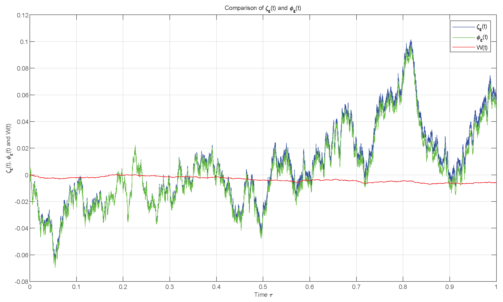
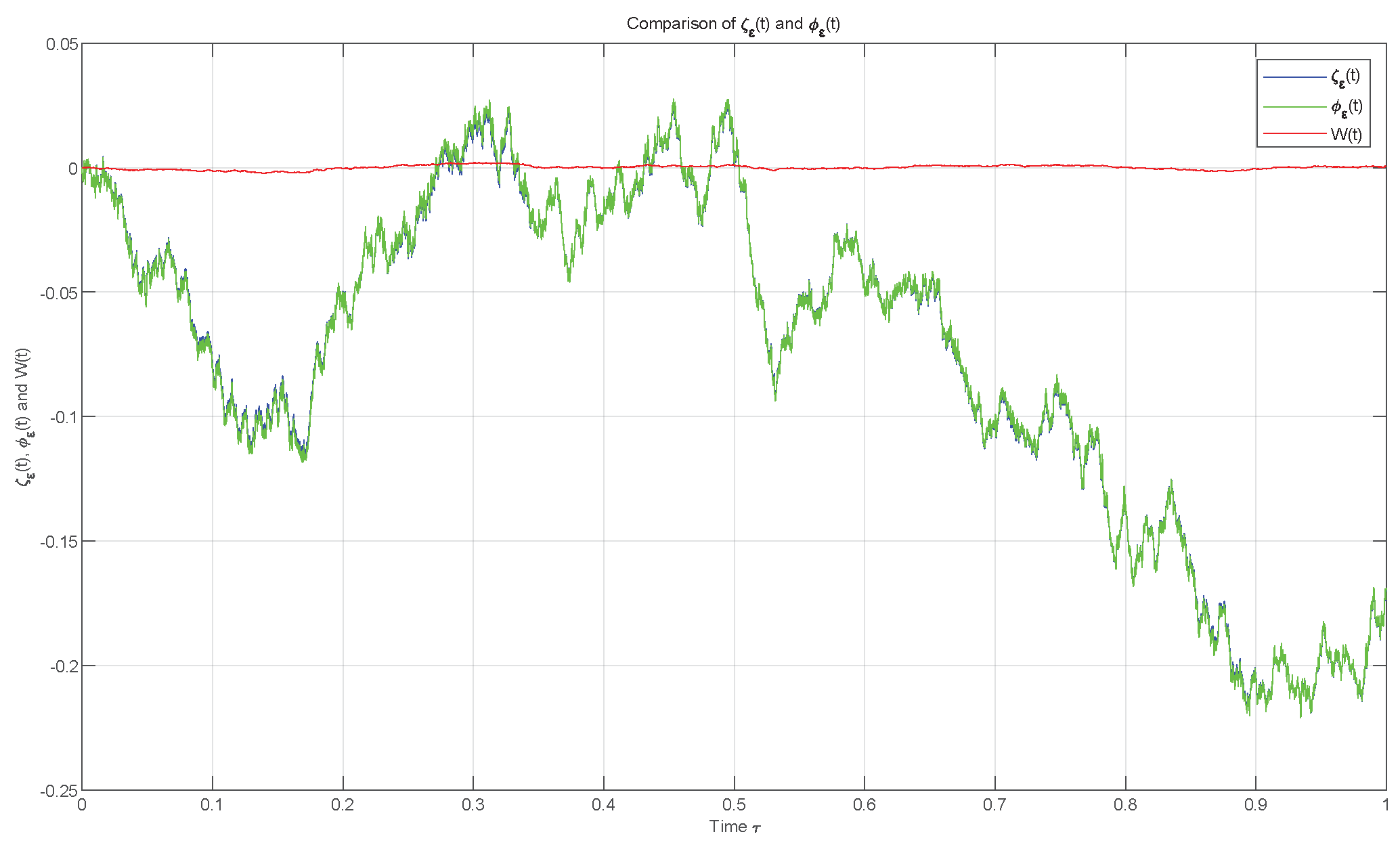
Then, it can be easily verified that the original Equation (21) and averaged Equation (22) satisfy conditions $\left(A_1\right)$–$\left(A_3\right)$. According to Theorem 1, we compare the error $W\left(t\right)=\parallel {\zeta }_{\epsilon }\left(\tau \right)-{\varphi }_{\epsilon }\left(\tau \right){\parallel }_{\mathbf{M}}^2$ between the solution ${\zeta }_{\epsilon }\left(\tau \right)$ of Equation (21) and the solution ${\varphi }_{\epsilon }\left(\tau \right)$ of Equation (22) for $\epsilon =0.01$ and $\epsilon =0.001$ on the interval $[0,1]$. See Figure 1 and Figure 2.

As $\epsilon \to 0$, we conclude that the solutions ${\zeta }_{\epsilon }\left(t\right)$ and ${\varphi }_{\epsilon }\left(t\right)$ are close in the mean square sense.

5. Conclusions

In this paper, we proposed a new equivalent form of Equation (1) through Lemma 3. The equivalent equation facilitates the construction of approximate solutions. Compared with existing literature, our work extends the applicability of averaging principles to fractional SDEs with discontinuous right-hand-side functions. Additionally, we prove that the convergence order between solutions is $2\alpha -1$, which is related to the fractional order. Numerical simulations validate the theoretical results. For future research, these results can be extended to higher-dimensional systems with multiplicative noise and stochastic control problems involving non-smooth dynamics.

References

1. Gu, H.; Trujillo, J.J. Existence of mild solution for evolution equation with Hilfer fractional derivative. Appl. Math. Comput. 2015, 257, 344–354. [Google Scholar] [CrossRef]
2. Pazy, A. Semigroups of Linear Operators and Applications to Partial Differential Equations; Springer: London, UK, 2012. [Google Scholar]
3. Kilbas, A.A.; Srivastava, H.M.; Trujillo, J.J. Theory and Applications of Fractional Differential Equations; Elsevier: Amsterdam, The Netherlands, 2006. [Google Scholar]
4. Rhaima, M.; Mchiri, L.; Makhlouf, A.B. Ulam type stability for mixed Hadamard and Riemann–Liouville fractional stochastic differential equations. Chaos Solitons Fract. 2024, 178, 114356. [Google Scholar] [CrossRef]
5. Khasminskii, R.Z. A limit theorem for the solutions of differential equations with random right-hand sides. Theory Probab. Appl. 1966, 11, 390–406. [Google Scholar] [CrossRef]
6. Maslowski, B.; Seidler, J.; Vrkoc, I. An averaging principle for stochastic evolution equations II. Math. Bohem. 1991, 116, 191–224. [Google Scholar] [CrossRef]
7. Xu, W.; Xu, W. An averaging principle for the time-dependent abstract stochastic evolution equations with infinite delay and Wiener process. J. Stat. Phys. 2020, 178, 1126–1141. [Google Scholar] [CrossRef]
8. Han, M.; Pei, B. An averaging principle for stochastic evolution equations with jumps and random time delays. AIMS Math. 2021, 6, 39–51. [Google Scholar] [CrossRef]
9. Abouagwa, M.; Aljoufi, L.S.; Bantan, R.A.R. Mixed neutral Caputo fractional stochastic evolution equations with infinite delay: Existence, uniqueness and averaging principle. Fractal. Fract. 2022, 6, 105. [Google Scholar] [CrossRef]
10. Yang, M.; Lv, T.; Wang, Q. The averaging principle for Hilfer fractional stochastic evolution equations with Lévy noise. Fractal. Fract. 2023, 7, 701. [Google Scholar] [CrossRef]
11. Liu, J.; Zhang, H.; Wang, J. A note on averaging principles for fractional stochastic differential equations. Fractal. Fract. 2024, 8, 216. [Google Scholar] [CrossRef]
12. Guo, Z.K.; Hu, J.H.; Yuan, C.G. Averaging principle for a type of Caputo fractional stochastic differential equations. Chaos 2021, 31, 053123. [Google Scholar] [CrossRef]
13. Pei, B.; Xu, Y.; Yin, G. Averaging principles for functional stochastic partial differential equations driven by a fractional Brownian motion modulated by two-time-scale Markovian switching processes. Nonlinear Anal. Hybrid Syst. 2018, 27, 107–124. [Google Scholar] [CrossRef]
14. Li, Z.; Yan, L. Stochastic averaging for two-time-scale stochastic partial differential equations with fractional Brownian motion. Nonlinear Anal. Hybrid Syst. 2019, 31, 317–333. [Google Scholar] [CrossRef]
15. Shen, G.; Xiang, J.; Wu, J.L. Averaging principle for distribution dependent stochastic differential equations driven by fractional Brownian motion and standard Brownian motion. J. Differ. Equ. 2022, 321, 381–414. [Google Scholar] [CrossRef]
16. Han, M.; Xu, Y.; Pei, B. Mixed stochastic differential equations: Averaging principle result. Appl. Math. Lett. 2021, 112, 106705. [Google Scholar] [CrossRef]
17. Lakshmikantham, V.; Bainov, D.D.; Simeonov, P.S. Theory of Impulsive Differential Equations; World Scientific: Singapore, 1989. [Google Scholar]
18. Shen, L.; Sun, J. Existence and uniqueness of solutions for stochastic impulsive differential equations. Stoch. Dyn. 2010, 10, 375–383. [Google Scholar] [CrossRef]
19. Lakhel, E.H.; Tlidi, A. Existence, uniqueness and stability of impulsive stochastic neutral functional differential equations driven by Rosenblatt process with varying-time delays. Rand. Oper. Stoch. Equ. 2019, 27, 213–223. [Google Scholar] [CrossRef]
20. Zou, J.; Luo, D.; Li, M. The existence and averaging principle for stochastic fractional differential equations with impulses. Math. Method. Appl. Sci. 2023, 46, 6857–6874. [Google Scholar] [CrossRef]
21. Ma, S.; Kang, Y. Periodic averaging method for impulsive stochastic differential equations with Lévy noise. Appl. Math. Lett. 2019, 93, 91–97. [Google Scholar] [CrossRef]
22. Khalaf, A.D.; Abouagwa, M.; Wang, X. Periodic averaging method for impulsive stochastic dynamical systems driven by fractional Brownian motion under non-Lipschitz condition. Adv. Differ. Equ. 2019, 2019, 526. [Google Scholar] [CrossRef]
23. Liu, J.; Wei, W.; Xu, W. An averaging principle for stochastic fractional differential equations driven by fBm involving impulses. Fractal. Fract. 2022, 6, 256. [Google Scholar] [CrossRef]
24. Tran, K.Q.; Yin, G. Exponential stability of stochastic functional differential equations with impulsive perturbations and Markovian switching. Syst. Control Lett. 2023, 173, 105457. [Google Scholar] [CrossRef]
25. Kao, Y.; Zhu, Q.; Qi, W. Exponential stability and instability of impulsive stochastic functional differential equations with Markovian switching. Appl. Math. Comput. 2015, 271, 795–804. [Google Scholar] [CrossRef]
26. Balasubramaniam, P. Hilfer fractional stochastic system driven by mixed Brownian motion and Lévy noise suffered by non-instantaneous impulses. Stoch. Anal. Appl. 2023, 41, 60–79. [Google Scholar] [CrossRef]
27. Mao, X. Stochastic Differential Equations and Application, 2nd ed.; Horwood Publishing Limited: Chichester, UK, 2007. [Google Scholar]
Figure 1. ζ ε ( t ) , ϕ ε ( t ) and W ( t ) with ζ 0 = 0 , ϕ 0 = 0 , ε = 0.01 , τ [ 0 , 1 ] .
Fractalfract 09 00340 g001
Figure 2. ζ ε ( t ) , ϕ ε ( t ) and W ( t ) with ζ 0 = 0 , ϕ 0 = 0 , ε = 0.001 , τ [ 0 , 1 ] .
Fractalfract 09 00340 g002
Disclaimer/Publisher’s Note: The statements, opinions and data contained in all publications are solely those of the individual author(s) and contributor(s) and not of MDPI and/or the editor(s). MDPI and/or the editor(s) disclaim responsibility for any injury to people or property resulting from any ideas, methods, instructions or products referred to in the content.