Graph-Based Stock Volatility Forecasting with Effective Transfer Entropy and Hurst-Based Regime Adaptation

Abstract

This study proposes a novel hybrid model for stock volatility forecasting by integrating directional and temporal dependencies among financial time series and market regime changes into a unified modeling framework. Specifically, we design a novel Hurst Exponent Effective Transfer Entropy Graph Neural Network (H-ETE-GNN) model that captures directional and asymmetric interactions based on Effective Transfer Entropy (ETE), and incorporates regime change detection using the Hurst exponent to reflect evolving global market conditions. To assess the effectiveness of the proposed approach, we compared the forecast performance of the hybrid GNN model with GNN models constructed using Transfer Entropy (TE), Granger causality, and Pearson correlation—each representing different measures of causality and correlation among time series. The empirical analysis was based on daily price data of 10 major country-level ETFs over a 19-year period (2006–2024), collected via Yahoo Finance. Additionally, we implemented recurrent neural network (RNN)-based models such as Long Short-Term Memory (LSTM) and Gated Recurrent Unit (GRU) under the same experimental conditions to evaluate their performance relative to the GNN-based models. The effect of incorporating regime changes was further examined by comparing the model performance with and without Hurst-exponent-based detection. The experimental results demonstrated that the hybrid GNN-based approach effectively captured the structure of information flow between time series, leading to substantial improvements in the forecast performance for one-day-ahead realized volatility. Furthermore, incorporating regime change detection via the Hurst exponent enhanced the model’s adaptability to structural shifts in the market. This study highlights the potential of H-ETE-GNN in jointly modeling interactions between time series and market regimes, offering a promising direction for more accurate and robust volatility forecasting in complex financial environments.

1. Introduction

Volatility prediction in financial markets is essential for various fields, such as portfolio optimization, risk management, and option pricing. Over the years, significant efforts have been made to develop reliable models that can accurately forecast market volatility. Traditionally, statistical time series models, such as Generalized Autoregressive Conditional Heteroskedasticity (GARCH), have predominantly been used for this purpose [1,2]. While GARCH models have proven effective in many contexts, recent advances have positioned deep learning algorithms at the forefront of volatility prediction [3]. In particular, Long Short-Term Memory (LSTM) models have gained prominence in the financial domain due to their ability to effectively capture long-term dependencies in time series data [4,5]. Despite the ability of deep learning models to effectively learn time series patterns, integrating domain knowledge is essential to account for the complexities and non-stationarity of financial markets [6]. While deep learning models have made significant strides, the integration of domain-specific knowledge remains a critical gap, especially in financial markets, where non-stationarity and regime shifts are prevalent. Models that are developed without a proper understanding of the specific characteristics of financial markets are at a higher risk of overfitting, which can undermine the generalizability of their predictive performance [7].

One of the primary challenges in volatility prediction in financial markets is regime changes, or shifts in market states. Markets experience alternating periods of economic growth and recession, each characterized by distinct volatility patterns. These changes can reduce the predictive power of models that do not consider regime changes. Consequently, various approaches that incorporate regime changes have been proposed. In particular, estimation of the time-varying Hurst exponent has received considerable attention as a way to capture long memory and structural changes in financial markets. To detect these changes, Melike and Özgür Ömer introduced a fractal-based GARCH model that accounts for long memory and volatility clustering [8]. Choi utilized the Hurst exponent through multifractal detrended fluctuation analysis (MFDFA) to assess dynamic market efficiency [9], and analyzed time-series variations in dynamic volatility spillovers to identify key points of market state transitions [10]. The Hurst exponent is a valuable tool for quantifying the long memory characteristics and autocorrelation structure of time series data, making it particularly effective in capturing the complex volatility patterns in financial markets [11]. In this context, Morales et al. proposed a dynamic Hurst exponent tool for monitoring unstable periods in financial time series [12]. Trinidad Segovia et al. employed the Hurst exponent via the fractal-based FD4 algorithm to detect volatility clusters [13]. Notably, the Hurst exponent can effectively detect non-stationarity and volatility clustering in markets, aiding in the identification of subtle patterns that traditional statistical models may overlook [14]. Eom et al. empirically investigated the relationship between market efficiency and the predictability of future price changes using the Hurst exponent [15]. Furthermore, the dynamic Hurst exponent, which evolves over time, can be used to track changes in financial market conditions in real-time, offering a more refined approach for detecting regime changes [16]. In these studies, wavelet-based estimators, parametric filtering techniques, and detrended fluctuation analysis (DFA/MFDFA) are frequently employed to estimate the time-varying Hurst exponent [17,18,19,20,21], each providing valuable insights into the dynamic structure of financial time series. According to the Fractal Market Hypothesis, the Hurst exponent, which reflects the multi-time scale characteristics of financial markets, plays a crucial role in identifying market instability and structural changes, thereby improving predictive accuracy across diverse market environments [22].

In addition to this perspective, recent literature on volatility modeling has proposed rough volatility models based on fractional Brownian motion (fBm), which suggest that the Hurst exponent is significantly smaller than $0.5$ when estimated on log-transformed realized volatility series [23,24,25]. These models challenge the traditional interpretation of long memory and suggest that volatility is rough, exhibiting anti-persistent behavior, rather than being persistent. While our approach does not adopt the log-transformation of high-frequency realized volatility, we instead compute the Hurst exponent of daily returns. This choice was motivated by empirical observations that the Hurst exponent of daily returns tends to fluctuate around $0.5$, allowing the detection of regime shifts as the market transitions between persistent ($H>0.5$) and anti-persistent ($H<0.5$) dynamics. For instance, during turbulent periods such as 2020, H consistently falls below $0.5$, aligning with a notable decrease in predictive performance. This suggests that the predictive difficulty associated with anti-persistent regimes, as also reported in the rough volatility literature [24], holds true in our empirical setting. While volatility estimates derived from daily returns are known to exhibit strong serial dependence, which may enhance predictability, we emphasize that this property is shared across all benchmark models used in our evaluation.

While regime changes describe temporal shifts, another important challenge in predicting volatility in financial time series is the structural interdependence among assets, influenced by various stakeholders. Stock prices are not determined in isolation; they are influenced by interactions with other stocks, exchange rates, and other economic factors [26]. The international financial market network is fully connected, strongly globalized, and intricately entangled, consisting of modular structures with similar efficiency dynamics [27]. Consequently, a model that simultaneously accounts for these financial stakeholders is essential, and various approaches have been proposed to address this issue. For example, Baltakys et al. proposed a graph neural network (GNN) approach to predict the trading behavior of socially connected investors, thereby enhancing market surveillance and detecting abnormal transactions [28]. Similarly, Chen and Robert utilized GNNs to model interactions between financial assets, which improves the accuracy of multivariate realized volatility forecasting [29]. Das et al. employed GNNs to model relationships among financial entities, integrating sentiment analysis to capture sentiment dynamics and structural dependencies [30]. Recent studies have increasingly adopted GNNs in financial forecasting, due to their ability to model complex relationships among financial entities. Unlike recurrent neural networks (RNN), GNNs reflect the relationships and structures between entities, making them a powerful tool for analyzing graph-structured data [31]. In particular, a Graph Convolutional Network (GCN), a prominent variation of GNNs, applies convolution operations to graph data to efficiently aggregate and propagate information from neighboring nodes [32]. These models are well suited for capturing relationships and interactions in complex network structures, making them particularly useful for analyzing multidimensional, interconnected data such as financial markets [33]. To effectively utilize GNN-based models, information about the interactions between entities is crucial, and various approaches have been developed to infer these relationships. Traditionally, statistical techniques and information theory have been used to measure correlation and causality. For example, Lu et al. presented a Pearson-correlation-based graph attention network that captures internal relationships between electroencephalography signal segments within brain regions to improve sleep stage classification [34]. Similarly, Jia and Benson proposed a framework that enhances GNN regression by modeling residual correlations using a parameterized multivariate Gaussian distribution, leading to improved prediction outcomes [35]. On the other hand, Wein et al. proposed a GNN-based causality network to infer causal relationships in brain networks, improving the accuracy of identifying directed dependencies between brain regions [36]. Zheng et al. developed a Granger causality-inspired graph neural network to model causal relationships in brain networks for interpretable psychiatric diagnosis [37]. Granger causality is a widely used technique for analyzing causality in time series data, assessing whether changes in one variable influence another [38]. However, this method can only determine the presence of information flow, and is limited when quantifying the magnitude or strength of the information transfer. To address this, research has been conducted using mutual information, based on information theory, to assess the quantity of information transferred. While mutual information is useful for measuring the dependence between two variables, it does not capture the directionality of the information flow. To overcome this limitation, Transfer Entropy (TE) was proposed, which is gaining attention as a metric that simultaneously estimates the direction and quantity of information transfer [39]. In line with this, Duan et al. presented a GNN that utilizes TE to capture causal relationships in multivariate time series, achieving superior forecasting performance across various real-world datasets [40]. However, TE can quantify causal relationships by measuring changes in probability distributions but suffers from issues related to finite sample effects and the presence of noise, which can degrade the accuracy of estimations [41]. To address these problems, Effective Transfer Entropy (ETE), which provides a more precise measurement of the direction and strength of information transfer, has been introduced [42].

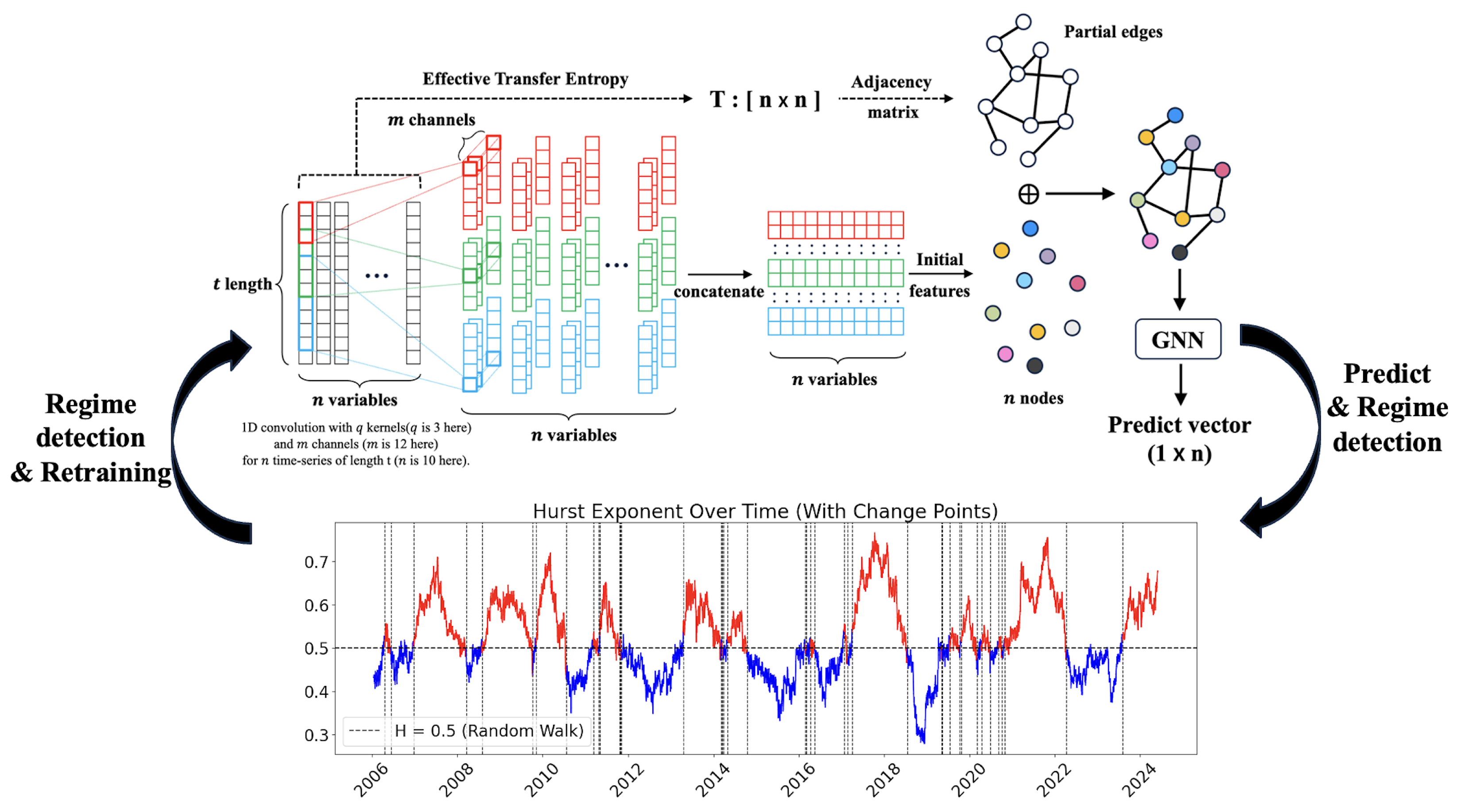
This study proposes a novel model that simultaneously considers the influence of multiple stakeholders, while adapting to regime changes by retraining the graph structure based on the Hurst exponent. First, the model quantifies information flows among ten country exchange-traded funds (ETFs) using effective transfer entropy. Second, it constructs a graph convolutional network utilizing ETE-based graphs to forecast one-day-ahead realized volatility. Third, the model detects regime changes through the Hurst exponent and dynamically retrains the graph when a regime change is identified. In comparison to prior works that relied on linear causality measures such as Granger causality or Pearson correlation, our approach captures nonlinear and directional causality more effectively through the use of ETE. Furthermore, we introduce a novel regime adaptation strategy that leverages the Hurst exponent to avoid unnecessary retraining during stable market trends, and focus updates only when structural changes are detected. The key contributions of this study are threefold. First, we develop a GNN-based forecasting framework that effectively captures nonlinear inter-asset dependencies by constructing adjacency matrices using ETE. Second, we propose a dynamic graph updating mechanism using the Hurst exponent, enabling the model to adapt to long-term memory dynamics and market regime shifts. Third, we empirically demonstrate that our hybrid model significantly outperformed various benchmarks, including GNNs using alternative causality measures and RNN-based models, in forecasting volatility over 19 years of ETF data. These results have practical implications for portfolio managers and risk analysts, as more accurate volatility forecasts can enhance asset allocation, hedging strategies, and option pricing. Theoretically, our framework advances the understanding of financial markets by integrating GNNs with nonlinear causality measures and a regime-adaptive mechanism based on the Hurst exponent, which captures varying memory characteristics across different market phases. The novelty of this study lies in being the first to integrate ETE-based graphs to capture collective dynamics among assets, while simultaneously accounting for regime changes using the Hurst exponent. Empirical results indicate that the proposed hybrid model improved the accuracy of realized volatility forecasts. These findings can contribute to a deeper understanding of fractal dynamics in financial markets, offering valuable insights for financial stakeholders.

The remainder of this paper is structured as follows: Section 2, which outlines the foundations of the ETE, causality graph neural network, and Hurst exponent; Section 3, which details the experimental approach and provides a statistical analysis of the financial time-series data; Section 4, which presents a comprehensive analysis of forecasting the realized volatility of ETFs; and Section 5, which interprets the findings and offers conclusions.

2. Methods

In order to forecast stock volatility more accurately, it is essential to consider the relationships between stocks and account for global regime changes. The ETE method was chosen because it effectively captures the directional causality among stocks, which is crucial for constructing a causality network that reflects the dynamic interconnections between different stocks [42]. GNNs can leverage the graph structure of the causality network to incorporate the relationships between different stocks into volatility forecasting [32]. Furthermore, the global stock market experiences episodic regime changes, which can be captured using the Hurst exponent [19]. The data included the daily closing prices of ten national ETFs, collected via Yahoo Finance. Log-returns were calculated, and the Hurst exponent was determined using a sliding window approach for global regime detection.

2.1. Effective Transfer Entropy

To understand ETE, it is essential to begin with the key concept of Mutual Information (MI) from information theory. MI is a measure that quantifies the statistical dependence between two random variables. Specifically, the MI between random variables X and Y, denoted as $I(X;Y)$, is defined as shown in Equation (1).

$$\begin{array}{cc}\hfill I(X;Y)& =H\left(X\right)+H\left(Y\right)-H(X,Y)\hfill \\ \hfill & =H\left(X\right)-H\left(X\mid Y\right)\hfill \end{array}$$

(1)

where $H\left(X\right)$ denotes the Shannon entropy of the random variable X, measuring the uncertainty of the probability distribution [43]. The conditional entropy $H\left(X\mid Y\right)$ represents the uncertainty of X given Y.

This concept of MI is extended to measure the causal relationship between time series, resulting in TE. TE measures the flow of information between two time series X and Y, quantifying the extent to which past values of Y contribute to predicting future values of X, and is defined as shown in Equation (2).

$$\begin{array}{cc}\hfill T{E}_{Y\to X}^{(k,l)}& =H(X_{t+1}\mid X_t^{\left(k\right)})-H(X_{t+1}\mid X_t^{\left(k\right)},Y_t^{\left(l\right)})\hfill \\ \hfill & =\sum _{i}p(x_{t+1},x_t^{\left(k\right)},y_t^{\left(l\right)})log{\displaystyle \frac{p(x_{t+1}\mid x_t^{\left(k\right)},y_t^{\left(l\right)})}{p(x_{t+1}\mid x_t^{\left(k\right)})}}\hfill \end{array}$$

(2)

where $x_t^{\left(k\right)}=\left(x_t,x_{t-1},\dots ,x_{t-k+1}\right)$ and $y_t^{\left(l\right)}=\left(y_t,y_{t-1},\dots ,y_{t-l+1}\right)$ represent the past k and l values of the times series X and Y, respectively. The conditional probability distribution $p(x_{t+1}\mid x_t^{\left(k\right)},y_t^{\left(l\right)})$ is used to measure how much better the probability of $x_{t+1}$ can be explained by incorporating the past information of Y along with that of X. Here, the sum is calculated over all possible joint combinations of $(x_{t+1},x_t^{\left(k\right)},y_t^{\left(l\right)})$, with i denoting the index for these joint combinations. In this study, following the approach in a previous work [44], we set the lag parameters k and l to 1, reflecting both theoretical and practical considerations. Theoretically, prior studies noted that stock markets in different time zones may experience delayed information transmission, and incorporating a one-day lag can better capture such cross-market dynamics. Practically, higher lag values exponentially increase the dimensionality of the conditional probability space, leading to greater computational complexity and estimation instability, especially in financial time series with limited data. As a result, TE is simplified as shown in Equation (3).

$$\begin{array}{cc}\hfill T{E}_{Y\to X}& =\sum _{i}p(x_{t+1},x_t,y_t)log{\displaystyle \frac{p(x_{t+1}\mid x_t,y_t)}{p(x_{t+1}\mid x_t)}}\hfill \end{array}$$

(3)

TE is calculated by estimating the conditional probability distribution between the past and future information of a time series. However, financial time series often contain high-frequency noise or extreme values, making it difficult to accurately estimate the continuous distribution. To address this issue, this study applied the Discretized Transfer Entropy method, which estimates the probability mass function through a discretization process [42]. Specifically, the time series segment for which TE is to be calculated is divided into proper intervals based on the maximum and minimum values, and the frequency of data points falling into each interval is measured to construct the probability mass function. Additionally, by constructing the joint probability distribution of the two time series in the same manner, all the conditional probabilities required for TE calculation can be estimated. This approach is useful for more reliably estimating the information flow in financial time series that include nonlinearity and noise. In this study, the number of intervals used for discretization was set to 3, following the approach in a previous study [42], where a ternary partition was adopted to represent the three fundamental types of price movements: significant gain, neutral or stable return, and significant loss. This discretization scheme provides an interpretable symbolic representation of market dynamics, while maintaining computational tractability in the estimation of Transfer Entropy [45].

On the other hand, while TE effectively captures nonlinear and asymmetric dependencies between time series, its application to real data may lead to overestimation or distorted interpretations, due to finite sample effects and the influence of noise. To address this, Marschinski and Kantz introduced the concept of ETE [42]. ETE is defined as shown in Equation (4), where the average TE value, calculated using randomized transfer entropy (RTE), is subtracted from the original TE in order to enhance the statistical significance of the TE value. The value of RTE is interpreted as a significance threshold, serving as a baseline to distinguish genuine information transfer from noise. To assess the statistical significance of the ETE value, we compute the Z-score based on the distribution of RTE, as shown in Equation (5). The Z-score measures how far the observed TE is from the mean of the shuffled TE values, normalized by their standard deviation. Only ETE values with a Z-score greater than $1.96$ are considered statistically significant.

$$\begin{array}{cc}\hfill ET{E}_{Y\to X}& =T{E}_{Y\to X}-{\displaystyle \frac{1}{m}}\sum _{i=1}^{m}T{E}_{Y_{\left(i\right)}\to X}\hfill \\ \hfill & =T{E}_{Y\to X}-{\mu }_{\mathrm{shuffled}Y\to X}\hfill \end{array}$$

(4)

$$Z={\displaystyle \frac{T{E}_{Y\to X}-{\mu }_{\mathrm{shuffled}Y\to X}}{{\sigma }_{\mathrm{shuffled}Y\to X}}}$$

(5)

where ${\mu }_{\mathrm{shuffled}Y\to X}$ and ${\sigma }_{\mathrm{shuffled}Y\to X}$ denote the mean and standard deviation of the transfer entropy values computed from m independently shuffled versions of Y to X. This filtering step mitigates the risk of overestimating spurious causality due to noise or finite sample effects, ensuring that only statistically robust information flows are preserved in the final ETE matrix. This process removes the temporal structure, while preserving the marginal distribution of the time series, thus destroying the causal relationship between variables [46]. Therefore, ETE adjusts the TE value to exclude information flows arising from mere chance or noise, reflecting only statistically significant information transmission. By considering both the direction and strength of information flow, while providing statistical control over randomness, ETE serves as a useful tool for financial time series analysis. As suggested by Marschinski and Kantz, multiple shuffle simulations are commonly used to stabilize the bias estimate [42]. While no fixed optimal number of shuffles is prescribed, several studies have used between 25 and 100 or more simulations [45,47,48]. In this study, the number of shuffle simulations was treated as a hyperparameter and hyperparameter tuning was conducted to identify the most effective value.

Meanwhile, to demonstrate the effectiveness of ETE, this study used traditional methods for measuring causality or correlation between two variables as benchmarks. One such method, Granger causality, evaluates whether past values of variable Y can predict future values of variable X, examining the potential causal relationship from Y to X [38]. To do this, a linear regression model, as shown in Equation (6), is set up, and the model’s predictive performance is tested by including past values of Y.

$$x_t=a_0+\sum _{i=1}^p{a}_i{x}_{t-i}+\sum _{j=1}^p{b}_j{y}_{t-j}+{ϵ}_t,$$

(6)

where $a_0$, ${\sum }_{i=1}^p{a}_i{x}_{t-i}$, ${\sum }_{j=1}^p{b}_j{y}_{t-j}$, p and ${ϵ}_t$ represent the constant term, autoregressive terms, exogenous terms, lag order, and error term, respectively. If the coefficients $b_j$ are statistically different from zero, this indicates that Y Granger causes X. However, Granger causality inherently assumes linearity and requires that the time series satisfy the condition of weak stationarity.

Another benchmark, Pearson correlation, is a statistical measure that quantifies the degree to which two variables, X and Y, change together linearly. The correlation coefficient ${\rho }_{X,Y}$ is defined as shown in Equation (7).

$${\rho }_{X,Y}={\displaystyle \frac{{\sum }_{i=1}^n(x_i-\overline{x})(y_i-\overline{y})}{\sqrt{{\sum }_{i=1}^n{(x_i-\overline{x})}^2}\sqrt{{\sum }_{i=1}^n{(y_i-\overline{y})}^2}}},$$

(7)

where $\overline{x}$ and $\overline{y}$ represent the mean values of X and Y, respectively, and n denotes the length of the time series. A Pearson correlation coefficient ${\rho }_{X,Y}$ close to 0 indicates a weak linear relationship, while a value near 1 or −1 indicates a strong positive or negative linear correlation, respectively. While Pearson correlation is useful for identifying simple linear relationships between variables, it has limitations: it cannot identify causal relationships, nor does it account for hidden common causes or non-linear structures.

In contrast, TE extends the causal concept of Granger causality from an information-theoretic perspective, offering the advantages of capturing non-linear relationships and measuring the direction of information flow. While Pearson correlation is a simple tool for correlation analysis, Granger causality, TE, and, most notably, the ETE used in this study, are focused on analyzing temporal causal structures or information flow. Specifically, TE and ETE differentiate themselves from Granger causality by evaluating the significance of information flow without assuming linearity.

2.2. Causality Graph Neural Network

GNNs are deep learning techniques designed to perform computations on graph-structured data [49]. By leveraging the structural relationships between nodes, GNNs can effectively solve node prediction tasks. The core of GNN training lies in the message passing mechanism, in which each node aggregates information from its neighboring nodes and updates its embedding vector accordingly. By repeating this process multiple times, GNNs are able to capture the structural dependencies between nodes in depth. In this study, we propose a model that predicts the one-day-ahead realized volatility of stocks by applying GNNs with adjacency matrices constructed based on ETE. Specifically, we estimate the statistically significant causal influence of one asset’s past information on the future volatility of another asset using ETE. Based on these causal relationships, we construct a sparse adjacency matrix that reflects only meaningful links between assets. Unlike fully connected graphs, where all nodes are linked, this approach builds a graph that only incorporates actual causal links, which reduces the model complexity and helps to minimize noise during training.

Time series data not only contain numerical information but also embody crucial temporal structures, such as periodicity. In particular, financial time series often exhibit fractal structures, demonstrating statistical self-similarity across various time scales. This means that statistical properties such as variance or autocorrelation may be preserved across different temporal resolutions. This characteristic highlights the importance of volatility forecasting, since capturing such scale-invariant statistical patterns is essential for modeling financial uncertainty. To effectively capture such characteristics, single-scale feature extraction is often insufficient. Therefore, this study employs multiple convolutional filters with different receptive fields to extract multi-scale features from time series data. These features are then concatenated and used as the initial node embeddings. Each convolutional filter $K_i$ has a distinct receptive field with a shape of $(1\times m_i)$, where $m_i$ is a predefined constant specifying the width of the receptive field for the i-th filter, and $i=0,1,\dots ,q$, with q denoting the number of filters used. Given a time series input v, the resulting initial node embedding f is computed as shown in Equation (8).

$$f=\underset{i=0}{\overset{q}{⨁}}\mathrm{ReLU}\left(K_i\ast v+b_i\right)$$

(8)

where ∗, ⨁, and $\mathrm{ReLU}\left(·\right)$ denote the convolution, concatenation, and rectified linear unit activation function $\mathrm{ReLU}\left(x\right)=max(0,x)$, respectively. In this framework, multivariate time series data are transformed into a feature matrix $H\in {\mathbb{R}}^{n\times d}$, where n and d denote the number of variables and the number of features, respectively. The adjacency matrix A between nodes is constructed based on the causality-driven methods described earlier. The message passing process in the GNN follows Equation (9).

$$h_i^{(l+1)}=\mathrm{ReLU}(h_i^{\left(l\right)}{W}_1^{\left(l\right)}+\sum _{j\in N\left(i\right)}{A}_{ji}{h}_j^{\left(l\right)}{W}_2^{\left(l\right)}),h^{\left(0\right)}=f.$$

(9)

where $W_1^{\left(l\right)}$ and $W_2^{\left(l\right)}$ are learnable weight matrices for the l-th layer, while $h_i^{\left(l\right)}$ and $h_j^{\left(l\right)}$ denote the hidden states of nodes i and j at layer l, respectively. $A_{ji}$ represents the weight of the directed edge from node j to node i, indicating the causal influence of node j on node i. $N\left(i\right)$ denotes the set of neighboring nodes of node i. In addition to integrating ETE into the GNN, this study also applied other causal inference methods, such as transfer entropy and Granger causality, as well as a correlation-based method, namely Pearson correlation, to construct the adjacency matrix, and compared their predictive performance.

2.3. Regime Detection Using Hurst Exponent

In this study, the Hurst exponent is used to analyze the fractal structure of time series data, identify structural changes, and define corresponding regimes. Reflecting the long-term memory and self-similarity of time series, the Hurst exponent represents its fractal characteristics and is widely recognized as an effective tool for interpreting the nonlinear and complex patterns of financial time series. In particular, rescaled range (R/S) analysis, which is employed to estimate the Hurst exponent, is a widely used method for quantitatively assessing the fractal characteristics of time series data [50].

Consider a time series $X=\{x_1,x_2,\dots ,x_n\}$, which is partitioned into segments of length w, resulting in a set of segments $X_w=\{T_1,T_2,\dots ,T_m\}$. Each segment $T_i$ is defined as $T_i=\{x_{(i-1)w+1},x_{(i-1)w+2},\dots ,x_{iw}\}$, where the total number of segments is $m=\lfloor {\displaystyle \frac{n}{w}}\rfloor$. By calculating the rescaled range $R/S$ for various scales w and analyzing the changes in the average $R/S$ values across these scales, the fractal scaling relationship of the time series can be determined. To accomplish this, the rescaled range value for each segment $T_i$ is determined by the procedure described below. Initially, the mean of each segment is calculated as given in Equation (10).

$$\overline{T_i}={\displaystyle \frac{1}{w}}\sum _{j=1}^w{x}_{(i-1)w+j}.$$

(10)

Subsequently, the cumulative deviation $Y_k^{\left(i\right)}$ from the segment mean is computed as shown in Equation (11).

$$Y_k^{\left(i\right)}=\sum _{j=1}^k(x_{(i-1)w+j}-\overline{T_i}),k=1,2,\dots ,w.$$

(11)

Next, the range $R_i$ for each segment is calculated by determining the difference between the maximum and minimum values of the cumulative deviation, as shown in Equation (12).

$$R_i=\underset{1\le k\le w}{max}\left\{Y_k^{\left(i\right)}\right\}-\underset{1\le k\le w}{min}\left\{Y_k^{\left(i\right)}\right\}.$$

(12)

Additionally, the standard deviation $S_i$ for each segment is calculated as shown in Equation (13).

$$S_i=\sqrt{{\displaystyle \frac{1}{w}}\sum _{j=1}^w{\left(X_{(i-1)w+j}-\overline{T_i}\right)}^2}.$$

(13)

The rescaled range is defined as $R_i/S_i$, and the average rescaled range for each scale w is calculated by averaging this value over all segments, as shown in Equation (14).

$${\left({\displaystyle \frac{R}{S}}\right)}_w={\displaystyle \frac{1}{m}}\sum _{i=1}^m{\displaystyle \frac{R_i}{S_i}}$$

(14)

The average $R/S$ value exhibits a specific pattern with respect to scale w, as shown in Equation (15), which generally follows a power law, indicating a fractal scaling relationship.

$${\left(R/S\right)}_w=c{w}^H.$$

(15)

where c is a constant and H is the Hurst exponent. Taking the logarithm of both sides yields a linear relationship, as shown in Equation (16).

$$log{\left(R/S\right)}_w=logc+Hlogw.$$

(16)

This can be interpreted as a linear regression model related to the fractal dimension. By fitting the relationship between $logw$ and $log{\left(R/S\right)}_w$ for multiple scales w using Ordinary Least Squares (OLS), the Hurst exponent can be estimated.

The Hurst exponent serves as a key numerical indicator of the fractality of a time series and enables interpretation of its dynamic properties according to its value. When H is close to $0.5$, the time series exhibits behavior similar to a random walk, implying the absence of serial dependence. A value of H greater than $0.5$ indicates a persistent structure with strong fractal autocorrelation, whereas a value less than $0.5$ reflects an anti-persistent structure, in which changes tend to occur in the opposite direction.

In this study, a Hurst exponent value of $0.5$ served as the criterion for regime classification. The value $0.5$ is commonly interpreted as the point where the time series behavior shifts from exhibiting persistent or anti-persistent characteristics to randomness, and it is often used to distinguish between regimes with long-term memory, random walk, and anti-persistent behavior [51,52]. A given time window is classified as a regime if the number of days on which the Hurst exponent exceeds $0.5$ is greater than or equal to a specified threshold s. Since slightly higher or lower values than $0.5$ can also produce meaningful results in empirical time series, several alternative thresholds—such as $0.45$ and $0.55$—were examined in a preliminary tuning phase. Additionally, a three-regime classification approach was also considered, where the regimes were defined as follows: Hurst exponent values below $0.45$, between $0.45$ and $0.55$, and above $0.55$. After a comprehensive evaluation of experimental results, a binary classification based on the $0.5$ threshold was selected, as it provided the best trade-off between interpretability and predictive performance. Details regarding the observation window and the threshold s for regime classification are presented in Section 3.1.

3. Experiments and Data

3.1. Experiments

This study proposes the H-ETE-GNN model to predict the realized volatility of ten national ETFs by incorporating causal relationships across countries and a global regime detection mechanism. This study used ten national ETFs, following the dataset configuration in Barua and Sharma (2021) [53]. These ETFs represent both developed and developing countries, providing a broad view of international equity markets. This selection supports the objective of modeling causal relationships across countries, which aligns with the proposed GNN framework. This study concentrated on national ETFs, rather than sectoral ETFs or other asset classes such as commodities or fixed income, in order to capture cross-country causal dynamics.

The overall experimental framework is presented in Figure 1. First, the close prices of the ten target national ETFs were collected to compute log-returns, which were used as inputs to construct the edge matrix, and the realized volatility values, which served as prediction targets. In addition, the log-return series of a representative world ETF was obtained, and the Hurst exponent was calculated using a sliding window approach. The window size was set to 250, since this setting produced a reasonable number of regime changes. With this window size, 47 regime changes were detected, while using 500 and 750 resulted in only 29 and 14 changes, respectively. These smaller counts may have been insufficient to adequately capture shifts in market conditions, so we chose 250, as it offered a more informative segmentation of the time series. To normalize the log-returns used as input features, min-max scaling was applied to rescale the values between zero and one. The GNN was trained using data from the most recent N days, which defined the training period. The edge matrix was also constructed based on these N days by estimating the directional causality among the ten national ETFs using the ETE method. For model training and evaluation, the training dataset was divided into two periods—training and validation—at a ratio of 7:3. A sliding window approach was employed during prediction, where the model took the most recent M days of information as input to forecast the next day’s realized volatility. Here, N refers to the length of the training period, and M denotes the input size of the model.

In the subsequent stage, if a regime change was detected, the GNN was retrained. The regime detection procedure was as follows. For the daily Hurst exponent of the world ETF, if the number of days with values exceeding $0.5$ during the past 10 days was greater than or equal to a threshold s, the current period was classified as an “Above” regime. Conversely, if the number of days with values below $0.5$ exceeded or equaled s, the period was classified as a “Below” regime. The threshold s served as a hyperparameter controlling the sensitivity of regime classification and was tuned through experimentation. When a regime shift was identified based on this criterion, the edge matrix was recalculated and the GNN was updated. Since the Hurst exponent reflected the memory and dependence structure in past observations, a detected regime shift indicated that structural changes had already been underway in the recent window. Therefore, although the detection point may coincide with the tail end of the previous regime, it already embeds early signs of the new regime’s characteristics, making it a reasonable point for fine-tuning the model. To reduce computational cost, the model was not fully retrained; instead, only the edge matrix was replaced, and the model was fine-tuned accordingly. On the other hand, if the regime remained unchanged, the previously trained model was directly used to predict the one-day-ahead realized volatility, without additional training.

In this study, three multi-scale convolutional filters were used to extract features from the time series data during the initialization of the GNN model. The lengths of each kernel were set to 3, 5, and 7 to capture both short-term and long-term temporal patterns simultaneously. The number of channels for each kernel was set to 12. Additionally, the GNN consisted of three layers, allowing for three iterations of message passing. The model was retrained every time a regime change was detected via the Hurst exponent, as shown in Figure 2. The lower part of Figure 2 presents the Hurst exponent over time, where regimes are alternately marked in red and blue to indicate regime changes. The objective function of the GNN model was the mean squared error (MSE), and the Adam optimizer was used for weight optimization. The activation function applied was ReLU, with 100 epochs and early stopping to prevent overfitting. Hyperparameter tuning was conducted using Bayesian optimization [54], and the hyperparameters used for tuning are listed in

Table 1. Hyperparameter tuning for GNNs.

Hyperparameter	Search Space
Learning rate	[1$\times {10}^{-2}$–1$\times {10}^{-5}$]
Batch size	$[4,8,16]$
Hidden state size of Nodes in layer 1	[10–100]
Hidden state size of Nodes in layer 2	[10–100]
Input size (M)	$[20,40,60]$
Training period (N)	$[250,500,750]$
Sensitivity of regime frequency (s)	$[6,7,8]$
Number of simulations for RTE (m) *	$[10\sim 100]$

Note: * is the hyperparameter only for ETE-GNN.

. For benchmarking, the RNN model was tuned with the hyperparameters specified in

Table 2. Hyperparameter tuning for RNNs.

Hyperparameter	Search Space
Learning rate	[1$\times {10}^{-2}$–1$\times {10}^{-5}$]
Batch size	$[4,8,16]$
Hidden size of Nodes in each layer	[10–100]
Number of layer	$[1,2,3,4,5]$
Drop out	[0–0.5]
Input size (M)	$[20,40,60]$
Training period (N)	$[250,500,750]$
Sensitivity of regime frequency (s)	$[6,7,8]$

, and the tuning results for the common hyperparameters M, N, and s are shown in

Table 3. Results of Hyperparameter tuning.

Hyperparameter	Result
Input size (M)	20
Training period (N)	750
Sensitivity of regime frequency (s)	6

.

For benchmarking, LSTM and Gated Recurrent Unit (GRU) models, which are widely used in time series forecasting, were adopted. LSTM, a variant of a RNN, effectively learns long-term dependencies through its input gate, forget gate, and output gate [55]. A GRU, proposed to alleviate the excessive complexity of LSTM while maintaining its performance, is used as well [56,57]. Since LSTM and GRU are not graph-based models, no separate causality matrix was used; instead, the past N-day log-return data of the ETFs were directly utilized to predict the realized volatility. During this process, regime detection and model retraining based on the Hurst exponent were performed. This allowed a comparison of the performance of the proposed H-ETE-GNN model with that of the LSTM and GRU models, as well as the evaluation of the predictive performance of a graph-based model that considered causality between countries. In addition, to assess the causality information encoded by ETE, benchmark GNN models were constructed using TE, Granger causality, and Pearson correlation to generate the edge matrix. When Granger causality was used to construct the edge matrix, the causality values were binarized into 0 and 1 based on a 5% significance level. In the case of Pearson correlation, only the magnitude of the correlation was considered by using the absolute correlation value. Furthermore, to evaluate the effectiveness of regime change detection, experiments were conducted on the aforementioned models without using the Hurst exponent, with the models being periodically retrained every N days during the training period.

Model performance was evaluated using Root Mean Squared Error (RMSE), Mean Absolute Error (MAE), Mean Absolute Percentage Error (MAPE), correlation, and Hit ratio. The implementation was carried out in Python 3.8.20 with PyTorch 2.0.0, and the experiments were conducted on a system with an AMD Ryzen 9 4.5 GHz processor, 32 GB of RAM, and an NVIDIA GTX 4090 with 24 GB of memory.

3.2. Data

The data for each ETF used in this study are presented in

Table 4. List of MSCI Country ETFs.

Ticker	MSCI Country ETFs
World	iShares MSCI World ETF
EWA	iShares MSCI Australia
EWC	iShares MSCI Canada
EWG	iShares MSCI Germany
EWJ	iShares MSCI Japan
EWT	iShares MSCI Taiwan
EWU	iShares MSCI United Kingdom
EWW	iShares MSCI Mexico
EWY	iShares MSCI South Korea
EWZ	iShares MSCI Brazil
EZA	iShares MSCI South Africa

. To comprehensively reflect the diverse stock price volatility across countries with differing macroeconomic conditions and market structures, 10 country ETFs representing both developed and emerging markets were selected. Since each ETF represents the overall market movement of the corresponding country’s stock market, they are useful for integrative analysis of various market dynamics observed across regions. For regime change detection, the Hurst exponent was calculated based on the time series of the iShares MSCI World ETF rather than individual countries. This ETF includes various regions and industrial sectors, reflecting global macroeconomic trends that extend beyond the market fluctuations of individual countries. By aggregating the stock markets of multiple developed nations into a single index, this provides a useful indicator for assessing the general direction of the global market, rather than focusing solely on specific countries. Therefore, the MSCI World index was used as a proxy for the Hurst exponent [58]. If the Hurst exponent were calculated separately for each country, the regime detection for each ETF would vary due to the heterogeneous market characteristics of each nation. This would result in different model retraining points for each ETF, significantly increasing the complexity and making it difficult to intuitively identify a common regime change. Thus, while realized volatility was predicted for each individual country ETF, the regime change detection relied solely on the MSCI World ETF, which reflects the overall market trends.

The Hurst exponent estimate provides more meaningful interpretation when the time series is stationary [59]. Therefore, the close price was converted into log return. The sample period was from 7 February 2003 to 29 May 2024. The log return, used as the model’s input, and the realized volatility, which served as the prediction target, were calculated as shown in Equations (17) and (18).

$$r_t=ln\left(p_t/p_{t-1}\right)$$

(17)

$${\mathrm{RV}}_t=\sqrt{{\displaystyle \frac{1}{n}}\sum _{i=1}^n{\left(100r_{t-i}\right)}^2}$$

(18)

where t refers to the specific date and n denotes the number of past observations. In this study, realized volatility was computed using the past 20 days of log returns. The log return at time t is denoted as $r_t$, and $p_t$ represents the closing price at time t.

Table 5. Descriptive statistics of each ETF.

ETF	Mean	Max	Min	Std.	Skewness	Kurtosis	Jarque-Bera Test	ADF Test 1
World	0.0003	0.1138	−0.1143	0.0122	−0.43	11.63	30,382.3 $*$	−18.0 $*$
EWA	0.0004	0.1885	−0.1756	0.0170	−0.40	13.76	42,430.8 $*$	−18.1 $*$
	1.4107	8.8432	0.4495	0.9523	3.85	20.24	104,378.4 $*$	−6.4 $*$
EWC	0.0003	0.1210	−0.1430	0.0139	−0.73	12.02	32,734.3 $*$	−14.0 $*$
	1.1754	6.9567	0.2797	0.7398	3.60	18.53	87,932.7 $*$	−6.3 $*$
EWG	0.0003	0.1806	−0.1357	0.0158	−0.2499	10.8642	26,425.98 $*$	−15.89 $*$
	1.3566	7.1317	0.3314	0.8108	3.04	13.13	46,587.8 $*$	−6.0 $*$
EWJ	0.0002	0.1469	−0.1099	0.0129	−0.0541	9.5307	20,296.35 $*$	−17.60 $*$
	1.1410	6.5646	0.2428	0.6101	3.64	21.64	115,961.8 $*$	−6.7 $*$
EWT	0.0003	0.1324	−0.1173	0.0161	−0.11	6.85	10,493.4 $*$	−14.3 $*$
	1.4247	6.9500	0.3769	0.7572	2.80	11.43	36,067.1 $*$	−5.4 $*$
EWU	0.0002	0.1576	−0.1281	0.0142	−0.5849	14.7663	49,020.56 $*$	−16.13 $*$
	1.1796	7.1011	0.3249	0.7886	3.49	16.94	74,691.7 $*$	−5.9 $*$
EWW	0.0004	0.1947	−0.1655	0.0171	−0.2500	9.5553	20,454.52 $*$	−15.91 $*$
	1.5051	7.8534	0.4583	0.8109	3.5113	18.00	83,056.8 $*$	−6.9 $*$
EWY	0.0003	0.2023	−0.1720	0.0191	0.1285	13.2797	39,414.09 $*$	−15.97 $*$
	1.6322	10.4741	0.5197	0.9981	4.31	26.05	167,526.7 $*$	−6.6 $*$
EWZ	0.0004	0.2278	−0.2626	0.0237	−0.6636	10.9457	27,160.56 $*$	−16.78 $*$
	2.0861	11.2281	0.5390	1.1278	4.13	24.64	150,277.7 $*$	−7.0 $*$
EZA	0.0003	0.2064	−0.2242	0.0213	−0.42	9.19	19,006.7 $*$	−16.7 $*$
	1.8931	10.1423	0.5694	0.9824	3.90	22.33	124,468.2 $*$	−7.1 $*$

Note: ¹ refers to the Augmented Dickey–Fuller Test, and * indicates the 1% level of significance. For each ETF, the top row shows the log-return data, while the bottom row presents the realized volatility data.

presents the descriptive statistics of the log returns and realized volatilities for each ETF. To examine the normality of the distributions, a Jarque–Bera test was conducted [60], and the augmented Dickey–Fuller (ADF) test was applied to assess the stationarity of the data [61]. Most log returns exhibit negative skewness, where this indicates that the left tail of the distribution is longer and large negative fluctuations are more probable. The kurtosis values are substantially higher than those of a normal distribution, where this suggests the presence of heavy tails and implies that extreme variations occur more frequently than under the normality assumption, which is a well-known characteristic of financial return time series. At the 1% significance level, the Jarque–Bera test rejected the null hypothesis of normality for all series, and the ADF test results indicated that all series were stationary.

Figure 3 illustrates the daily Hurst exponent calculated using the World ETF. Also, Hurst exponent is color-coded in alternating red and blue to indicate each regime shift. The sensitivity of regime frequency was set to 6, as determined by the experiment that yielded the best performance. Each vertical dashed line in the figure marks a detected regime change, with a total of 47 changes observed. Consequently, the proposed model, H-ETE-GNN, was retrained 47 times accordingly.

4. Results

To evaluate the predictive performance of the proposed model, three analytical approaches were employed. First, the validity of regime detection using the Hurst exponent was assessed to determine whether it contributed to improved forecasting accuracy. Second, the effectiveness of the GNN in capturing and analyzing the structural relationships among the ten ETFs was verified through ETE, a statistical measure that estimates the directional flow of information between time series. To this end, the results were comprehensively compared and analyzed against benchmark models, with particular attention paid to year-by-year performance differences and the impact of each factor on model predictions. The model’s predictive performance was evaluated using RMSE, MAE, MAPE, and correlation, as defined by the following equations. In addition to those, we report the hit ratio, which measures the percentage of times the predicted direction matched the actual direction.

$$\begin{array}{cc}\hfill \mathrm{RMSE}& =\sqrt{{\displaystyle \frac{1}{n}}\sum _{i=1}^n{\left({\widehat{y}}_i-y_i\right)}^2},\hfill \end{array}$$

(19)

$$\begin{array}{cc}\hfill \mathrm{MAE}& ={\displaystyle \frac{1}{n}}\sum _{i=1}^n\left|{\widehat{y}}_i-y_i\right|,\hfill \end{array}$$

(20)

$$\begin{array}{cc}\hfill \mathrm{MAPE}& ={\displaystyle \frac{1}{n}}\sum _{i=1}^n\left|{\displaystyle \frac{{\widehat{y}}_i-y_i}{y_i}}\right|\times 100,\hfill \end{array}$$

(21)

$$\begin{array}{cc}\hfill \mathrm{Corr}(y,\widehat{y})& ={\displaystyle \frac{{\sum }_{i=1}^n(y_i-\overline{y})({\widehat{y}}_i-\overline{\widehat{y}})}{\sqrt{{\sum }_{i=1}^n{(y_i-\overline{y})}^2}\sqrt{{\sum }_{i=1}^n{({\widehat{y}}_i-\overline{\widehat{y}})}^2}}}.\hfill \end{array}$$

(22)

$$\begin{array}{cc}\hfill \mathrm{Hit}\mathrm{Ratio}& ={\displaystyle \frac{1}{n-1}}\sum _{i=2}^n\mathbb{I}\left[sign({\widehat{y}}_i-{\widehat{y}}_{i-1})=sign(y_i-y_{i-1})\right]\hfill \end{array}$$

(23)

where n, $y_i$, ${\widehat{y}}_i$, $\overline{y}$, and $\overline{\widehat{y}}$ represent the total number of samples, the real value, the predicted value, the mean of the real values, and the mean of the predicted values, respectively. The operator $sign\left(·\right)$ returns the sign of a value (i.e., 1 if positive, 0 if zero, and $-1$ if negative), and $\mathbb{I}\left[·\right]$ the indicator function, which returns 1 if the condition inside the brackets is true, and 0 otherwise.

4.1. Forecasting Performance by Model

To evaluate the effectiveness of regime detection using the Hurst exponent,

Table 6. Comparison of Periodic changes vs. Hurst regimes; best results are highlighted in bold.

Regime	Model	RMSE	MAE	MAPE	Correlation	Hit Ratio
Periodic	LSTM	$0.5136\pm 0.0159$	$0.3489\pm 0.0104$	$22.3469\pm 0.7976$	$0.6913\pm 0.0225$	$0.5882\pm 0.0073$
	GRU	$0.4598\pm 0.0330$	$0.3112\pm 0.0169$	$19.9726\pm 0.6166$	$0.7545\pm 0.0141$	$0.6137\pm 0.0113$
	Pearson-GNN	$0.2162\pm 0.0125$	$0.1495\pm 0.0059$	$10.2881\pm 0.1839$	$0.9514\pm 0.0042$	$0.7010\pm 0.0160$
	Granger-GNN	$0.1858\pm 0.0136$	$0.1231\pm 0.0074$	$8.2433\pm 0.4123$	$0.9509\pm 0.0042$	$0.7027\pm 0.0109$
	TE-GNN	$0.2142\pm 0.0166$	$0.1455\pm 0.0101$	$9.9158\pm 0.5892$	$0.9552\pm 0.0049$	$0.7082\pm 0.0287$
	ETE-GNN	$0.2001\pm 0.0077$	$0.1301\pm 0.0051$	$8.4759\pm 0.4749$	$0.9565\pm 0.0030$	$0.7040\pm 0.0074$
Hurst	LSTM	$0.5008\pm 0.0227$	$0.3381\pm 0.0144$	$21.2038\pm 0.7920$	$0.6993\pm 0.0295$	$0.5995\pm 0.0104$
	GRU	$0.4494\pm 0.0618$	$0.3059\pm 0.0398$	$19.6617\pm 1.9591$	$0.7337\pm 0.0656$	$0.6166\pm 0.0196$
	Pearson-GNN	$0.2021\pm 0.0129$	$0.1371\pm 0.0050$	$9.1044\pm 0.1768$	$0.9471\pm 0.0027$	$0.6904\pm 0.0142$
	Granger-GNN	$0.1833\pm 0.0387$	$0.1118\pm 0.0143$	$6.9656\pm 0.6217$	$0.9595\pm 0.0057$	$0.7091\pm 0.0133$
	TE-GNN	$0.1973\pm 0.0171$	$0.1309\pm 0.0107$	$8.5549\pm 0.7052$	$0.9535\pm 0.0055$	$\mathbf{0}.\mathbf{7213}\pm \mathbf{0}.\mathbf{0115}$
	ETE-GNN	$\mathbf{0}.\mathbf{1623}\pm \mathbf{0}.\mathbf{0166}$	$\mathbf{0}.\mathbf{1024}\pm \mathbf{0}.\mathbf{0091}$	$\mathbf{6}.\mathbf{6555}\pm \mathbf{0}.\mathbf{6552}$	$\mathbf{0}.\mathbf{9605}\pm \mathbf{0}.\mathbf{0060}$	$0.7206\pm 0.0087$

compares periodic retraining with Hurst-based regime retraining. ETE-GNN, TE-GNN, Granger-GNN, and Pearson-GNN denote models that employed ETE, TE, Granger causality, and Pearson correlation, respectively, to construct the edge matrix of the GNN. The comparison included both RNNs, specifically LSTM and GRU models, and the GNN models under the two retraining strategies. All experiments were repeated ten times, and both the average and standard deviation were reported to ensure the reliability of the results. The results indicate that regime detection using the Hurst exponent consistently led to improved performance in all GNN-based models. Notably, H-ETE-GNN achieved the best performance among all models. Under the periodic regime, Granger-GNN showed the lowest error rates among all models. While regime detection also improved the performance in LSTM and GRU, the degree of improvement was relatively modest compared to the GNN-based models. In addition, both LSTM and GRU exhibited relatively high RMSE and MAPE values, and their correlation coefficients remained below $0.76$. Overall, regime detection based on the Hurst exponent proved effective across all GNN-based architectures, including H-ETE-GNN. Moreover, models that incorporated relational information among multiple time series outperformed those that relied solely on individual series. Among them, H-ETE-GNN, which utilized ETE, demonstrated the highest level of predictive accuracy. In terms of hit ratio, the Hurst-based TE-GNN achieved the highest value at $0.7213$, but the Hurst-based ETE-GNN also recorded a comparable score of $0.7206$, with no statistically significant difference between the two models.

Table 7. p-Value for pairwise comparison.

Regime	Pairwise Comparison	RMSE	MAE	MAPE	Correlation	Hit Ratio
Periodic	ETE-GNN vs. LSTM	<0.0001	<0.0001	<0.0001	<0.0001	<0.0001
	ETE-GNN vs. GRU	<0.0001	<0.0001	<0.0001	<0.0001	<0.0001
	ETE-GNN vs. Pearson-GNN	0.0017	<0.0001	<0.0001	0.0031	0.3020
	ETE-GNN vs. Granger-GNN	0.9941	0.9871	0.8712	0.0018	0.3795
	ETE-GNN vs. TE-GNN	0.0152	0.0004	<0.0001	0.2432	0.6704
Hurst	ETE-GNN vs. LSTM	<0.0001	<0.0001	<0.0001	<0.0001	<0.0001
	ETE-GNN vs. GRU	<0.0001	<0.0001	<0.0001	<0.0001	<0.0001
	ETE-GNN vs. Pearson-GNN	<0.0001	<0.0001	<0.0001	<0.0001	<0.0001
	ETE-GNN vs. Granger-GNN	0.0699	0.0493	0.1460	0.3537	0.0185
	ETE-GNN vs. TE-GNN	<0.0001	<0.0001	<0.0001	0.0075	0.5592
Hurst vs. Periodic	LSTM	0.0811	0.0348	0.0024	0.2531	0.0060
	GRU	0.3233	0.3524	0.3209	0.8248	0.3471
	Pearson-GNN	0.0113	<0.0001	<0.0001	0.9916	0.9339
	Granger-GNN	0.4254	0.0223	<0.0001	0.0008	0.1275
	TE-GNN	<0.0001	0.0029	0.0001	0.7543	0.1039
	ETE-GNN	<0.0001	<0.0001	<0.0001	0.0408	0.0001

Note: bold indicate statistically significant differences in pairwise comparisons at the 5% level based on one-tailed t-tests.

presents the results of the one-tailed t-tests conducted to evaluate the statistical significance of performance differences between ETE-GNN and existing models. The table lists pairwise comparisons across three settings: between ETE-GNN and other models under the Periodic regime, under the Hurst-based regime detection, and between models with and without regime detection. In the Periodic regime, ETE-GNN consistently achieved a better performance than the RNN-based models across all metrics and showed statistically significant improvements over Pearson-GNN in terms of RMSE and correlation. In contrast, no significant differences were observed between ETE-GNN and Granger-GNN, indicating comparable performance. ETE-GNN showed superiority over TE-GNN only in RMSE and MAE. Under the Hurst-based regime, ETE-GNN outperformed LSTM, GRU, Pearson-GNN, and TE-GNN across all metrics, with strong statistical significance, and also showed clear superiority over Granger-GNN in MAE and hit ratio. In comparisons between the Hurst-based and Periodic settings, ETE-GNN showed significant improvements across all metrics, while LSTM, Pearson-GNN, and TE-GNN also exhibited meaningful improvements in specific metrics. These findings suggest that the Hurst-exponent-based regime detection strategy effectively contributed to improving the performance of ETE-GNN, while also providing measurable benefits for other models.

To examine whether splitting regimes based on the Hurst exponent around $0.5$ was optimal, this study also explored a ternary regime detection scheme using three ranges of H values.

Table 8. Comparison of Periodic changes vs. Hurst regimes: Ternary Regimes; best results are highlighted in bold.

Regime	Model	RMSE	MAE	MAPE	Correlation	Hit Ratio
Periodic	LSTM	$0.5273\pm 0.0293$	$0.3591\pm 0.0197$	$23.1487\pm 1.3677$	$0.6817\pm 0.0351$	$0.5888\pm 0.0143$
	GRU	$0.4501\pm 0.0310$	$0.3046\pm 0.0170$	$19.6434\pm 0.9358$	$0.7656\pm 0.0229$	$0.6224\pm 0.0201$
	Pearson-GNN	$0.2118\pm 0.0125$	$0.1448\pm 0.0071$	$9.8856\pm 0.4464$	$0.9563\pm 0.0045$	$0.7054\pm 0.0198$
	Granger-GNN	$0.1805\pm 0.0169$	$0.1223\pm 0.0108$	$8.3726\pm 0.7512$	$0.9578\pm 0.0061$	$0.7167\pm 0.0145$
	TE-GNN	$0.2164\pm 0.0230$	$0.1488\pm 0.0131$	$10.3996\pm 0.8008$	$0.9529\pm 0.0056$	$0.6906\pm 0.0210$
	ETE-GNN	$0.1922\pm 0.0184$	$0.1335\pm 0.0043$	$8.4740\pm 0.9299$	$0.9570\pm 0.0027$	$0.7037\pm 0.0109$
Hurst	LSTM	$0.4833\pm 0.0233$	$0.3229\pm 0.0165$	$20.2248\pm 0.7979$	$0.7050\pm 0.0276$	$0.6001\pm 0.0097$
	GRU	$0.4586\pm 0.0511$	$0.3038\pm 0.0227$	$18.9682\pm 0.8370$	$0.7492\pm 0.0279$	$0.6193\pm 0.0166$
	Pearson-GNN	$0.2015\pm 0.0108$	$0.1335\pm 0.0043$	$8.7634\pm 0.1912$	$0.9485\pm 0.0038$	$0.7072\pm 0.0094$
	Granger-GNN	$0.1933\pm 0.0341$	$0.1192\pm 0.0156$	$7.3380\pm 0.5441$	$0.9624\pm 0.0049$	$0.7328\pm 0.0153$
	TE-GNN	$0.1937\pm 0.0279$	$0.1247\pm 0.0107$	$8.1341\pm 0.5742$	$0.9399\pm 0.0069$	$0.7106\pm 0.0117$
	ETE-GNN	$\mathbf{0}.\mathbf{1677}\pm \mathbf{0}.\mathbf{0203}$	$\mathbf{0}.\mathbf{1066}\pm \mathbf{0}.\mathbf{0122}$	$\mathbf{6}.\mathbf{9536}\pm \mathbf{0}.\mathbf{8295}$	$\mathbf{0}.\mathbf{9646}\pm \mathbf{0}.\mathbf{0065}$	$\mathbf{0}.\mathbf{7359}\pm \mathbf{0}.\mathbf{0125}$

presents the experimental results using a ternary regime detection scheme based on the Hurst exponent. Each model operated under identical experimental settings, applied to both the Periodic-change and Hurst-based regime detection frameworks. The ternary regime detection approach classified each time window into three regimes according to the Hurst exponent: the Below regime when the Hurst value is below $0.45$, indicating anti-persistent behavior; the Middle regime, when it lies between $0.45$ and $0.55$; and the Above regime, when it exceeds $0.55$, indicating persistent trends. The difference in prediction performance between the binary and ternary regime detection methods remained small. The binary approach identified 47 regime changes, while the ternary approach identified 57, based on hyperparameter settings that yielded the best performance in each case. Although the more fine-grained ternary classification aimed to capture a richer representation of market states, the experimental results did not indicate a significant performance gain compared to the simpler binary approach and instead introduced additional computational overhead. This study adopted the binary regime detection method as the final strategy, considering both interpretability and computational efficiency.

Figure 4 illustrates the edge matrices used at the initial training stage for each GNN model. The edge matrix based on Pearson correlation broadly captured the correlation structure among assets; however, its overly dense connectivity tended to degrade the prediction performance. In contrast, the matrix constructed using Granger causality strictly filtered the edges based on statistical significance, resulting in a highly sparse structure. While this sparsity prevented overfitting, it also removed potentially informative connections, limiting predictive gains. The adjacency matrix derived from TE fell between Pearson and ETE in terms of sparsity, reflecting meaningful information flow, while avoiding excessive linkage. The matrix based on ETE, which subtracted RTE from TE, further eliminated statistically insignificant edges, leading to a sparser but more informative structure. This enabled the model to more effectively capture essential information flow across assets. As a result, the model utilizing ETE demonstrated the highest predictive accuracy, followed closely by the model using Granger causality. These findings highlight that avoiding both overly dense and overly sparse structures, while accurately reflecting relationships among assets, is crucial for improving volatility forecasting performance.

Figure 5 presents the predicted time series of models with Hurst-exponent-based regime detection, compared to the actual realized volatility. During periods of sharp volatility spikes, such as the 2008 global financial crisis and the 2020 COVID pandemic, the predicted trends from the models diverged significantly. Across all periods, the GNN-based models such as ETE-GNN, TE-GNN, Granger-GNN, and Pearson-GNN generally provided predictions close to the actual values. In contrast, the RNN-based models such as LSTM and GRU tended to either overestimate or underestimate the volatility in certain periods, with this tendency being most pronounced during sharp increases in volatility.

4.2. Forecasting Performance by Period

To thoroughly evaluate the predictive performance of the proposed model, we examined the annual prediction results.

Table 9. RMSE of prediction results with Hurst exponent by year; best results are highlighted in bold.

Year	ETE-GNN	TE-GNN	Granger-GNN	Pearson-GNN	GRU	LSTM
2006	0.093576	0.120988	0.107847	0.150821	0.251559	0.360012
2007	0.138237	0.155003	0.119717	0.19180	0.358143	0.414321
2008	0.528721	0.265332	0.363093	0.350294	1.071818	1.31239
2009	0.130072	0.189313	0.16203	0.206066	0.480808	0.606376
2010	0.097381	0.130098	0.184585	0.186329	0.319448	0.385758
2011	0.108857	0.131685	0.141575	0.179691	0.303854	0.372681
2012	0.079983	0.095109	0.092748	0.136270	0.196815	0.222060
2013	0.085781	0.116787	0.087138	0.159504	0.249111	0.312822
2014	0.092161	0.126627	0.114354	0.317552	0.334894	0.138842
2015	0.072724	0.104604	0.085149	0.302509	0.335230	0.142492
2016	0.114217	0.189315	0.136153	0.409397	0.411964	0.207057
2017	0.081223	0.101730	0.094578	0.218263	0.295346	0.131794
2018	0.074196	0.117100	0.111772	0.276600	0.335285	0.141714
2019	0.057191	0.078074	0.078111	0.161840	0.194780	0.100395
2020	0.279826	0.337985	0.410608	0.738375	0.769176	0.283386
2021	0.097534	0.116206	0.096964	0.204433	0.229905	0.119735
2022	0.165068	0.191153	0.128979	0.295869	0.342428	0.202757
2023	0.092029	0.102919	0.074890	0.193309	0.218770	0.115690
2024	0.064914	0.073564	0.073252	0.157016	0.220153	0.086697
ALL	0.128991	0.147395	0.139473	0.169092	0.338264	0.418793

compares the annual RMSE values of models with Hurst-exponent-based regime detection. Overall, the proposed H-ETE-GNN demonstrated the best performance, but its results were less favorable during the periods of the 2008 financial crisis and the COVID pandemic. This was due to the infrequent occurrence of regime changes during these periods. According to Figure 3, there were two regime changes between 2007 and 2008, while only one regime change occurred between 2021 and 2023. Over 19 years, there were 47 regime changes, making these periods below average in terms of regime changes. If an incorrect network was learned and no regime change occurred, the prediction performance in those periods deteriorated. Furthermore, although ETE was introduced to address the shortcomings of TE, ETE had limitations in capturing extreme non-linear interactions [62]. During these periods, ETE’s failure to capture extreme non-linear patterns and the lack of regime change resulted in suboptimal predictions. Meanwhile, the Granger-GNN model, which was relatively simple and effective in capturing linear relationships, performed better during these periods. In conclusion, the proposed H-ETE-GNN performed outstandingly during periods of low volatility, but its performance was relatively lower during the high-volatility periods of the 2007–2008 financial crisis and the 2020–2023 COVID-19 pandemic.

Figure 6, Figure 7, Figure 8 and Figure 9 present the annual prediction performance of each model, corresponding to RMSE, MAE, MAPE, and correlation metrics, respectively. For each model, the results of Hurst regime detection and periodic changes were averaged and displayed as annual charts. Overall, the GNN models exhibited superior predictive performance compared to the RNN models, with the RNN models showing a tendency to significantly increase errors during periods of sharp market fluctuations. The proposed H-ETE-GNN model demonstrated a stable prediction performance across most periods, indicating that ETE effectively captured the information flow between time series.

Next, we examined the effectiveness of Hurst-exponent-based regime detection by analyzing annual prediction performance.

Table 10. RMSE of H-ETE-GNN and ETE-GNN; best results are highlighted in bold.

Year	H-ETE-GNN	ETE-GNN
2006	0.093576	0.115425
2007	0.138237	0.132837
2008	0.528721	0.400041
2009	0.130072	0.163219
2010	0.097381	0.100169
2011	0.108857	0.147067
2012	0.079983	0.073312
2013	0.085781	0.114265
2014	0.092161	0.101416
2015	0.072724	0.085714
2016	0.114217	0.082246
2017	0.068729	0.119254
2018	0.071846	0.076547
2019	0.052705	0.061678
2020	0.329050	0.235567
2021	0.083982	0.121108
2022	0.144332	0.158366
2023	0.074686	0.190886
2024	0.060439	0.069389
ALL	0.128991	0.135264

presents the annual RMSE results for H-ETE-GNN and ETE-GNN. In all years, except for 2008, 2012, and 2020, H-ETE-GNN demonstrated superior performance. In 2012, the difference between the two models was minimal, while in 2008 and 2020, ETE-GNN showed better performance. As mentioned earlier, this may occur in periods where regime changes are infrequent.

To further assess the broad applicability of Hurst-exponent-based regime detection,

Table 11. RMSE comparison: Hurst-exponent-based regime detection vs. Periodic changes; best results are highlighted in bold.

Year	Hurst	Periodic
2006	0.188091	0.181199
2007	0.204936	0.203966
2008	0.295798	0.296016
2009	0.237579	0.243642
2010	0.195083	0.205760
2011	0.170849	0.185416
2012	0.151699	0.165340
2013	0.170993	0.165369
2014	0.159629	0.171022
2015	0.129706	0.144976
2016	0.185998	0.199404
2017	0.170929	0.168490
2018	0.199629	0.219936
2019	0.136258	0.144142
2020	0.310456	0.325601
2021	0.142529	0.156203
2022	0.184521	0.189637
2023	0.114369	0.125710
2024	0.123529	0.140107
ALL	0.223708	0.238767

presents the annual RMSE from a collective perspective. For all RNN and GNN models, the average RMSE values under both Hurst regime detection and periodic changes were calculated. The results show that, in certain periods, the periodic changes model slightly outperformed, which may indicate that regime detection’s advantages are less clear in market environments where fluctuations are not extreme or during specific phases. Nevertheless, in general, the application of regime detection resulted in better performance. This suggests that the Hurst-exponent-based regime detection method effectively captured market phase changes, regardless of the predictive model used.

Finally, the effectiveness of GNNs considering causality between countries was examined.

Table 12. RMSE of GNN and RNN; best results are highlighted in bold.

Year	GNN	RNN
2006	0.123901	0.295199
2007	0.167630	0.396877
2008	0.395544	1.182893
2009	0.177603	0.550174
2010	0.130343	0.372061
2011	0.157550	0.438664
2012	0.106249	0.207390
2013	0.137923	0.285685
2014	0.117996	0.326223
2015	0.101242	0.318869
2016	0.161685	0.410681
2017	0.102331	0.256804
2018	0.111196	0.305943
2019	0.078443	0.178310
2020	0.327951	0.753776
2021	0.107610	0.217169
2022	0.171989	0.319148
2023	0.096382	0.206040
2024	0.074263	0.188584
ALL	0.153018	0.387370

compares the annual RMSE averages of GNN models and RNN models. In every year, the GNNs significantly outperformed the RNNs, demonstrating that GNNs are better at capturing the structural information of financial markets.

5. Discussion and Conclusions

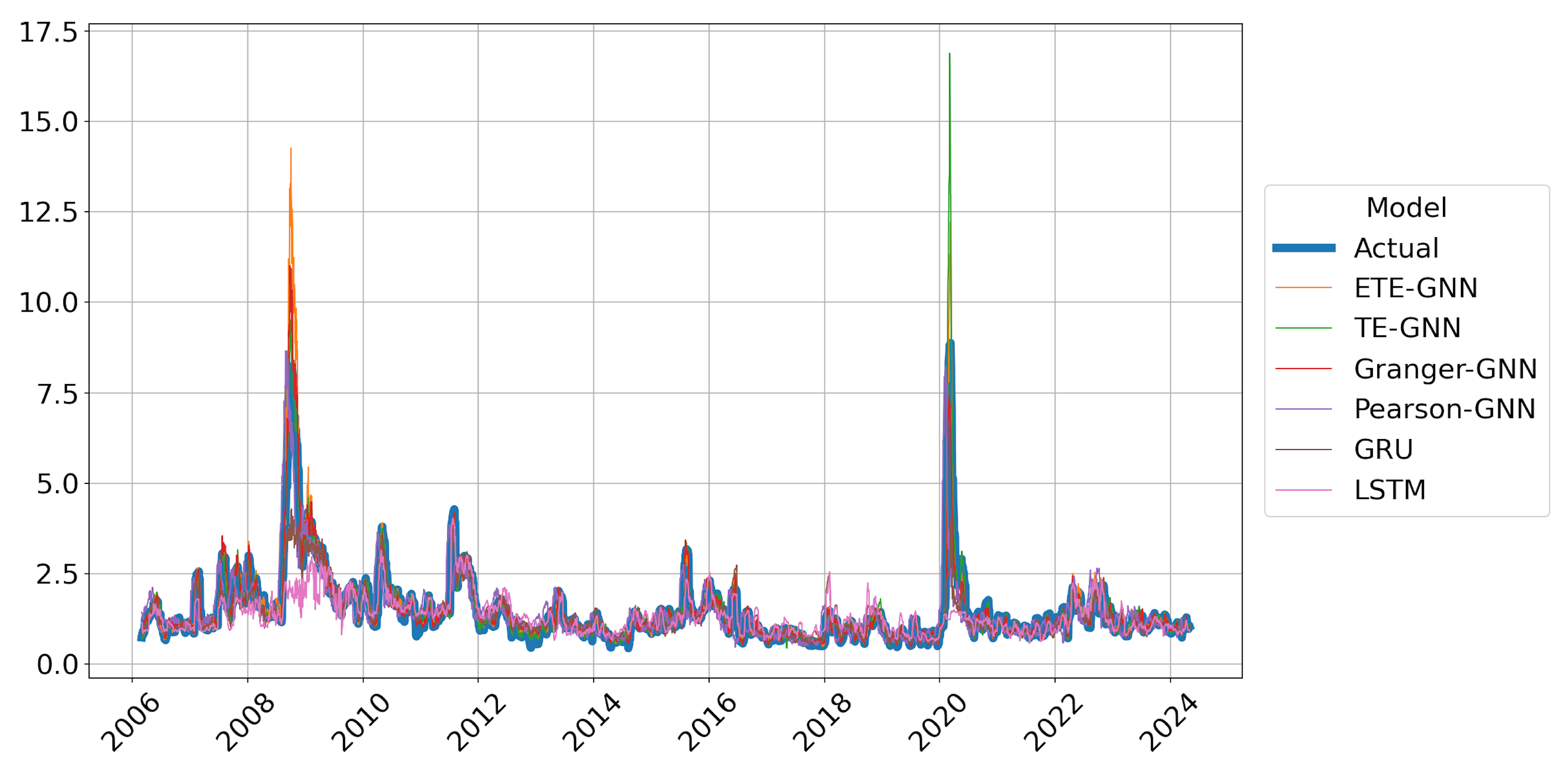
This paper introduces a hybrid model, H-ETE-GNN, which combines the ETE to estimate nonlinear inter-asset causality with GNNs, while dynamically reflecting market regime changes using the Hurst exponent. The primary contributions of this study are clearly outlined as follows: First, a framework is developed that effectively analyzes data structures reflecting inter-asset causality through an adjacency matrix composed of ETE. By utilizing this approach, GNNs can interpret the network structure of financial markets and systematically analyze the impact of interactions between nodes on prediction performance, unlike traditional RNN models based on sequential learning. Second, the study introduces a strategy that monitors the long-term dependency characteristics of financial markets using the Hurst exponent. By detecting regime changes based on this, the model dynamically retrains the ETE graph and parameters, demonstrating the potential for a prediction system that adapts flexibly to structural market fluctuations. Third, the effectiveness of the proposed H-ETE-GNN was validated by analyzing 19 years of data from 10 national ETFs. When compared to various benchmark models, the H-ETE-GNN showed superior performance in volatility forecasting, confirming its applicability. In addition to these contributions, the novelty of our work lies in the comprehensive comparison against benchmark models. In contrast to prior works that relied on linear causality measures, such as Granger causality or Pearson correlation, our approach highlighted the superior ability of the GNN model based on ETE to capture nonlinear and directional causality. Moreover, the incorporation of Hurst-exponent-based regime change detection adds significant value, enhancing the model’s adaptability to shifting market dynamics.

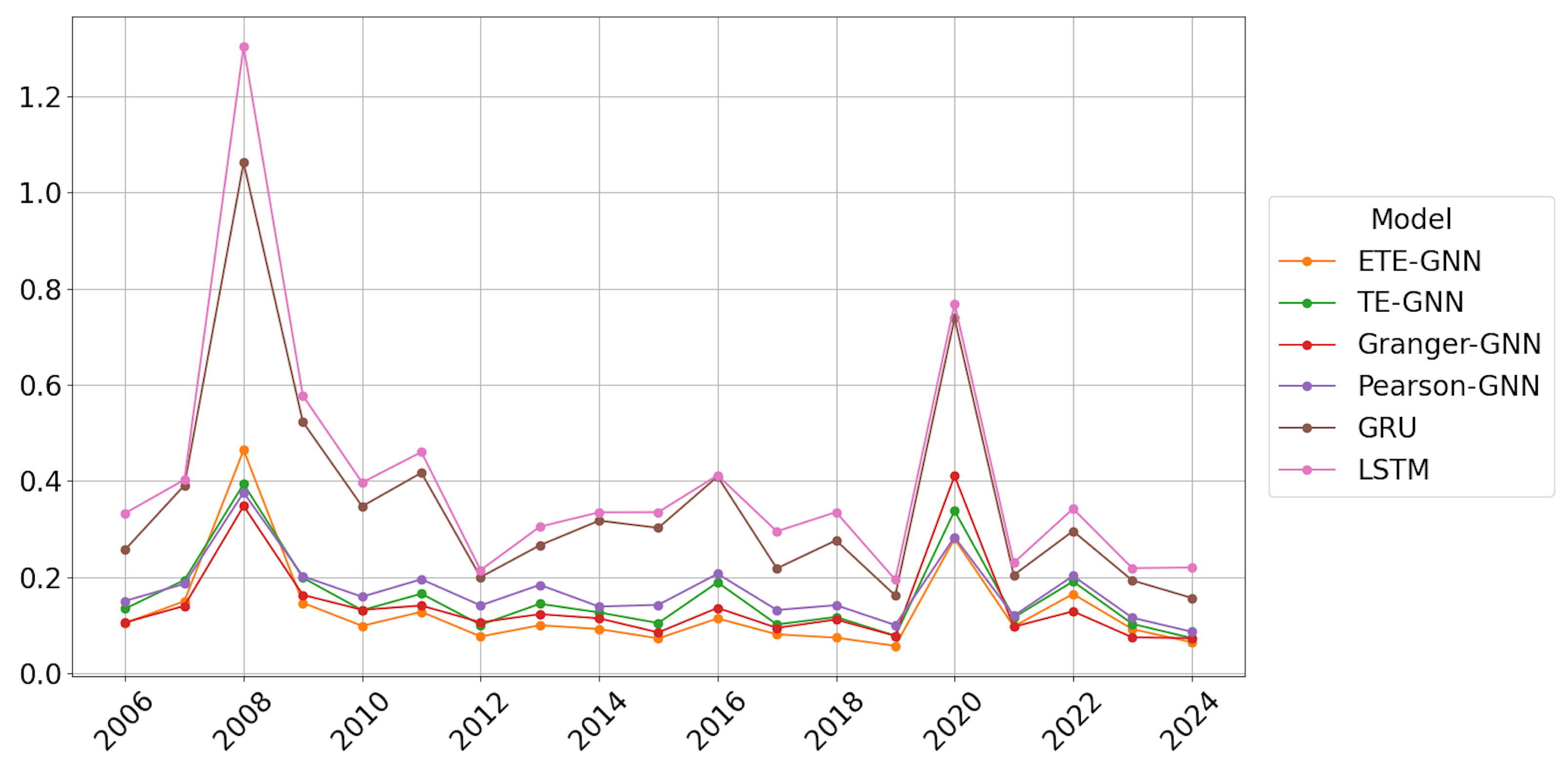
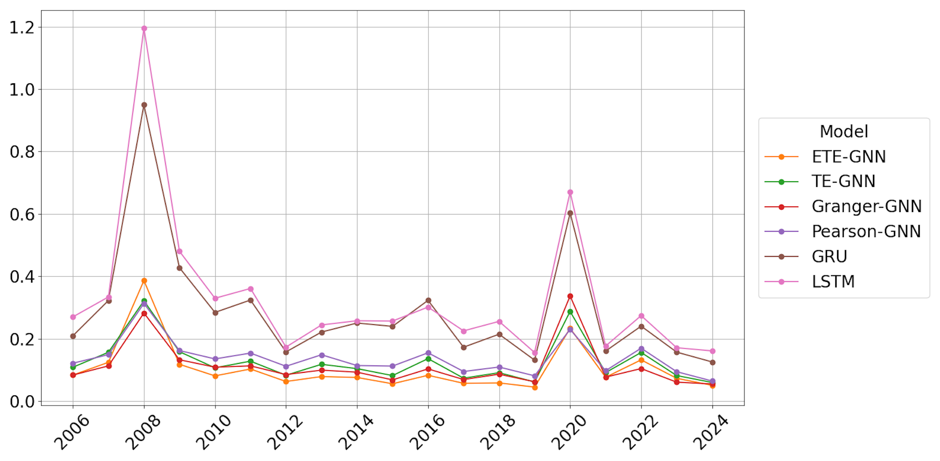
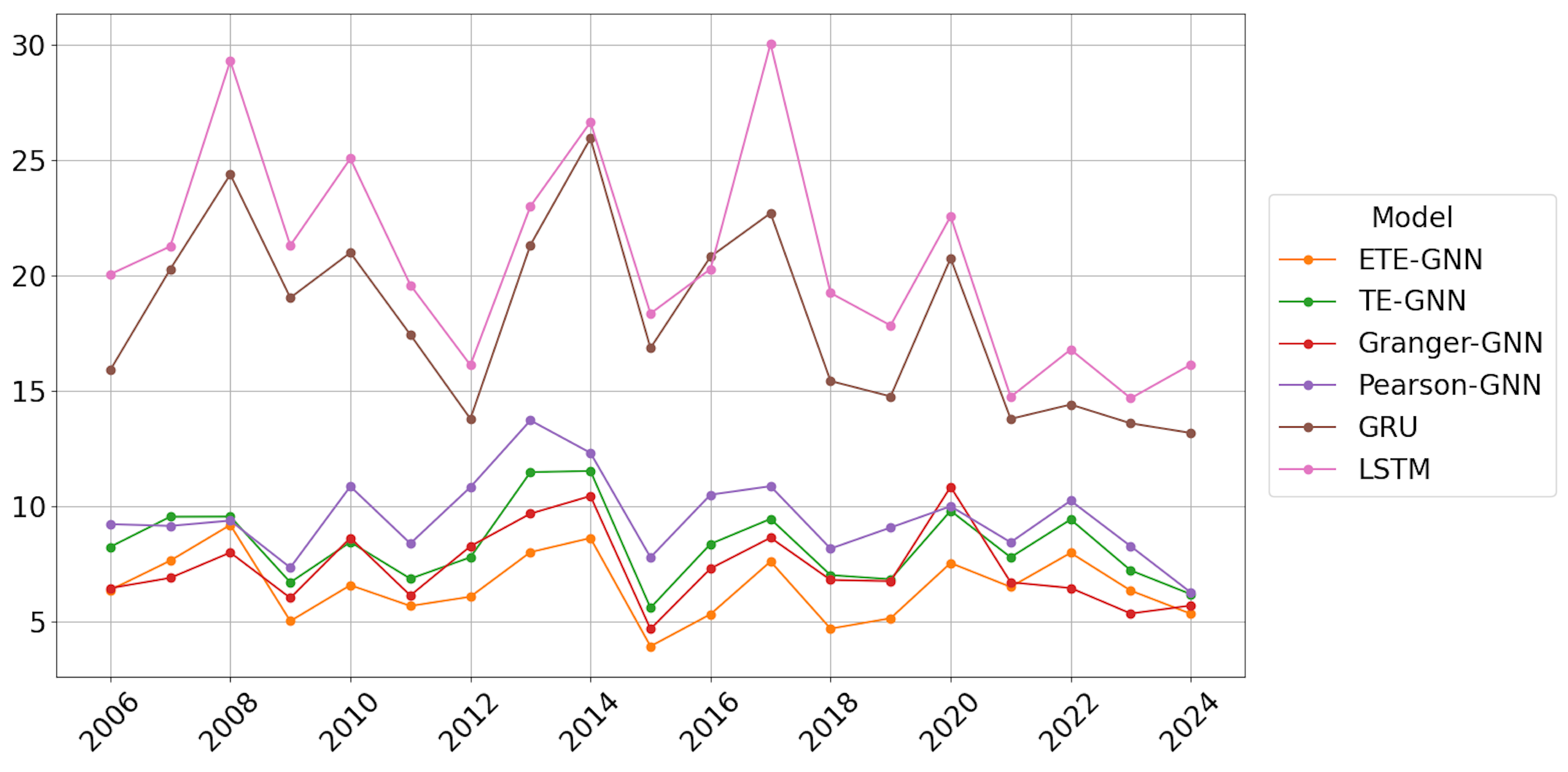
In this study, a series of benchmark experiments revealed that the GNN model based on ETE outperformed those based on TE, Granger causality, and Pearson correlation. This highlights that ETE’s ability to effectively capture nonlinear information flow contributes to improved prediction performance. Furthermore, when compared to RNN-based models under the same conditions, the GNN-based models, which reflected structural interactions between assets, generally demonstrated superior performance. Additionally, the strategy incorporating Hurst-exponent-based regime change detection outperformed Periodic retraining, underscoring the value of adapting models to long-term memory dependencies in the market.

The proposed H-ETE-GNN efficiently balances both accuracy and effectiveness by avoiding unnecessary retraining during stable market trends and only retraining at regime change points. This adaptive mechanism allows for more efficient deployment in real-world systems where computational resources are limited, and market dynamics are highly variable. However, during periods of rapid market collapse, such as the 2008 financial crisis or the 2020 COVID-19 pandemic, the model’s performance temporarily deteriorated. This suggests that the current modeling approach, while effective under typical conditions, has limitations in capturing abrupt and extreme market behaviors. This can be attributed to the fact that the Hurst exponent operates under a monofractal assumption, which may not fully capture the asymmetric and complex nature of the market structure. Additionally, while ETE improves causal inference compared to traditional TE, it has limitations in detecting extreme, localized nonlinear interactions, potentially missing crucial regime changes. These findings imply that, although H-ETE-GNN offers a promising solution for volatility forecasting in complex markets, its current structure may need further enhancement to deal with sudden and extreme market fluctuations and rapidly changing dependency structures. Thus, future research should focus on developing algorithms that can sensitively incorporate event significance or extreme probabilities to enhance causal inference stability during extreme market conditions. Recent studies have suggested that asymmetric multifractal Hurst exponents positively impact volatility forecasting [4], and the potential use of Rényi-entropy-based Transfer Entropy to better capture key information flow has also been explored [63]. Building on these advancements, future work could focus on hybridizing H-ETE-GNN with asymmetric multifractal analysis and Renyi transfer entropy, thereby increasing its robustness and adaptability across diverse market regimes, including crises. Another promising future direction involves incorporating high-frequency financial data to estimate realized volatility more accurately. While our current model relies on daily-return-based volatility estimates, applying ETE and GNN techniques to realized volatility derived from intraday data may improve responsiveness and granularity, particularly during volatile or rapidly evolving market conditions. Additionally, future research could explore integrating past volatility values directly into the model architecture. While our current GNN framework is designed around return-based node features, incorporating volatility information may enhance prediction performance if implemented carefully. To avoid potential overfitting due to increased input dimensionality, a hybrid approach such as LSTM-GNN could be adopted to jointly capture temporal and cross-sectional dependencies—an extension that lies beyond the scope of the present study but offers a promising avenue for future work.

References

1. Franses, P.H.; Van Dijk, D. Forecasting stock market volatility using (non-linear) Garch models. J. Forecast. 1996, 15, 229–235. [Google Scholar] [CrossRef]
2. Sen, J.; Mehtab, S.; Dutta, A. Volatility Modeling of Stocks from Selected Sectors of the Indian Economy Using GARCH. In Proceedings of the 2021 Asian Conference on Innovation in Technology (ASIANCON), Pune, India, 27–29 August 2021; pp. 1–9. [Google Scholar] [CrossRef]
3. Kim, H.Y.; Won, C.H. Forecasting the volatility of stock price index: A hybrid model integrating LSTM with multiple GARCH-type models. Expert Syst. Appl. 2018, 103, 25–37. [Google Scholar] [CrossRef]
4. Cho, P.; Lee, M. Forecasting the Volatility of the Stock Index with Deep Learning Using Asymmetric Hurst Exponents. Fractal Fract. 2022, 6, 394. [Google Scholar] [CrossRef]
5. Sivadasan, E.T.; Mohana Sundaram, N.; Santhosh, R. Stock market forecasting using deep learning with long short-term memory and gated recurrent unit. Soft Comput. 2024, 28, 3267–3282. [Google Scholar] [CrossRef]
6. Ahmed, D.M.; Hassan, M.M.; Mstafa, R.J. A Review on Deep Sequential Models for Forecasting Time Series Data. Appl. Comput. Intell. Soft Comput. 2022, 2022, 6596397. [Google Scholar] [CrossRef]
7. Hommes, C.H. Financial markets as nonlinear adaptive evolutionary systems. Quant. Financ. 2001, 1, 149. [Google Scholar] [CrossRef]
8. Bildirici, M.; Ersin, Ö.Ö. Regime-Switching Fractionally Integrated Asymmetric Power Neural Network Modeling of Nonlinear Contagion for Chaotic Oil and Precious Metal Volatilities. Fractal Fract. 2022, 6, 703. [Google Scholar] [CrossRef]
9. Choi, S.Y. Analysis of stock market efficiency during crisis periods in the US stock market: Differences between the global financial crisis and COVID-19 pandemic. Phys. A Stat. Mech. Its Appl. 2021, 574, 125988. [Google Scholar] [CrossRef]
10. Choi, S.Y. Dynamic volatility spillovers between industries in the US stock market: Evidence from the COVID-19 pandemic and Black Monday. N. Am. J. Econ. Financ. 2022, 59, 101614. [Google Scholar] [CrossRef]
11. Hurst, H.E. Long-term storage capacity of reservoirs. Trans. Am. Soc. Civ. Eng. 1951, 116, 770–799. [Google Scholar] [CrossRef]
12. Morales, R.; Di Matteo, T.; Gramatica, R.; Aste, T. Dynamical generalized Hurst exponent as a tool to monitor unstable periods in financial time series. Phys. A Stat. Mech. Its Appl. 2012, 391, 3180–3189. [Google Scholar] [CrossRef]
13. Trinidad Segovia, J.; Fernández-Martínez, M.; Sánchez-Granero, M. A novel approach to detect volatility clusters in financial time series. Phys. A Stat. Mech. Its Appl. 2019, 535, 122452. [Google Scholar] [CrossRef]
14. Tzouras, S.; Anagnostopoulos, C.; McCoy, E. Financial time series modeling using the Hurst exponent. Phys. A Stat. Mech. Its Appl. 2015, 425, 50–68. [Google Scholar] [CrossRef]
15. Eom, C.; Choi, S.; Oh, G.; Jung, W.S. Hurst exponent and prediction based on weak-form efficient market hypothesis of stock markets. Phys. A Stat. Mech. Its Appl. 2008, 387, 4630–4636. [Google Scholar] [CrossRef]
16. Endres, S.; Stübinger, J. A flexible regime switching model with pairs trading application to the S&P 500 high-frequency stock returns. Quant. Financ. 2019, 19, 1727–1740. [Google Scholar] [CrossRef]
17. Simonsen, I.; Hansen, A.; Nes, O.M. Determination of the Hurst exponent by use of wavelet transforms. Phys. Rev. E 1998, 58, 2779–2787. [Google Scholar] [CrossRef]
18. Carbone, A.; Castelli, G.; Stanley, H. Time-dependent Hurst exponent in financial time series. Phys. A Stat. Mech. Its Appl. 2004, 344, 267–271, Applications of Physics in Financial Analysis 4 (APFA4). [Google Scholar] [CrossRef]
19. Gómez-Águila, A.; Trinidad-Segovia, J.; Sánchez-Granero, M. Improvement in Hurst exponent estimation and its application to financial markets. Financ. Innov. 2022, 8, 86. [Google Scholar] [CrossRef]
20. Peng, C.K.; Buldyrev, S.V.; Havlin, S.; Simons, M.; Stanley, H.E.; Goldberger, A.L. Mosaic organization of DNA nucleotides. Phys. Rev. E 1994, 49, 1685–1689. [Google Scholar] [CrossRef]
21. Kantelhardt, J.W.; Zschiegner, S.A.; Koscielny-Bunde, E.; Havlin, S.; Bunde, A.; Stanley, H. Multifractal detrended fluctuation analysis of nonstationary time series. Phys. A Stat. Mech. Its Appl. 2002, 316, 87–114. [Google Scholar] [CrossRef]
22. Doorasamy, M.; Sarpong, P. Fractal market hypothesis and Markov regime switching model: A possible synthesis and integration. Int. J. Econ. Financ. Issues 2018, 8, 93–100. [Google Scholar]
23. Gatheral, J.; Jaisson, T.; Rosenbaum, M. Volatility is rough. Quant. Financ. 2018, 18, 933–949. [Google Scholar] [CrossRef]
24. Garcin, M. Forecasting with fractional Brownian motion: A financial perspective. Quant. Financ. 2022, 22, 1495–1512. [Google Scholar] [CrossRef]
25. Wang, X.; Yu, J.; Zhang, C. On the optimal forecast with the fractional Brownian motion. Quant. Financ. 2024, 24, 337–346. [Google Scholar] [CrossRef]
26. Summer, M. Financial Contagion and Network Analysis. Annu. Rev. Financ. Econ. 2013, 5, 277–297. [Google Scholar] [CrossRef]
27. Cho, P.; Kim, K. Global Collective Dynamics of Financial Market Efficiency Using Attention Entropy with Hierarchical Clustering. Fractal Fract. 2022, 6, 562. [Google Scholar] [CrossRef]
28. Baltakys, K.; Baltakienė, M.; Heidari, N.; Iosifidis, A.; Kanniainen, J. Predicting the trading behavior of socially connected investors: Graph neural network approach with implications to market surveillance. Expert Syst. Appl. 2023, 228, 120285. [Google Scholar] [CrossRef]
29. Chen, Q.; Robert, C.Y. Multivariate Realized Volatility Forecasting with Graph Neural Network. In Proceedings of the Third ACM International Conference on AI in Finance, New York, NY, USA, 2–4 November 2022; ICAIF ’22. pp. 156–164. [Google Scholar] [CrossRef]
30. Das, N.; Sadhukhan, B.; Chatterjee, R.; Chakrabarti, S. Integrating sentiment analysis with graph neural networks for enhanced stock prediction: A comprehensive survey. Decis. Anal. J. 2024, 10, 100417. [Google Scholar] [CrossRef]
31. Scarselli, F.; Gori, M.; Tsoi, A.C.; Hagenbuchner, M.; Monfardini, G. The Graph Neural Network Model. IEEE Trans. Neural Netw. 2009, 20, 61–80. [Google Scholar] [CrossRef]
32. Kipf, T.N.; Welling, M. Semi-Supervised Classification with Graph Convolutional Networks. arXiv 2017. [Google Scholar] [CrossRef]
33. Wang, J.; Zhang, S.; Xiao, Y.; Song, R. A Review on Graph Neural Network Methods in Financial Applications. arXiv 2022. [Google Scholar] [CrossRef]
34. Lu, J.; Tian, Y.; Wang, S.; Sheng, M.; Zheng, X. PearNet: A Pearson Correlation-based Graph Attention Network for Sleep Stage Recognition. In Proceedings of the 2022 IEEE 9th International Conference on Data Science and Advanced Analytics (DSAA), Shenzhen, China, 13–16 October 2022; pp. 1–8. [Google Scholar] [CrossRef]
35. Jia, J.; Benson, A.R. Residual Correlation in Graph Neural Network Regression. In Proceedings of the 26th ACM SIGKDD International Conference on Knowledge Discovery & Data Mining, New York, NY, USA, 6–10 July 2020; KDD ’20. pp. 588–598. [Google Scholar] [CrossRef]
36. Wein, S.; Malloni, W.M.; Tomé, A.M.; Frank, S.M.; Henze, G.I.; Wüst, S.; Greenlee, M.W.; Lang, E.W. A graph neural network framework for causal inference in brain networks. Sci. Rep. 2021, 11, 8061. [Google Scholar] [CrossRef] [PubMed]
37. Zheng, K.; Yu, S.; Chen, B. CI-GNN: A Granger causality-inspired graph neural network for interpretable brain network-based psychiatric diagnosis. Neural Netw. 2024, 172, 106147. [Google Scholar] [CrossRef] [PubMed]
38. Granger, C.W.J. Investigating Causal Relations by Econometric Models and Cross-spectral Methods. Econometrica 1969, 37, 424–438. [Google Scholar] [CrossRef]
39. Schreiber, T. Measuring Information Transfer. Phys. Rev. Lett. 2000, 85, 461–464. [Google Scholar] [CrossRef]
40. Duan, Z.; Xu, H.; Huang, Y.; Feng, J.; Wang, Y. Multivariate Time Series Forecasting with Transfer Entropy Graph. Tsinghua Sci. Technol. 2023, 28, 141–149. [Google Scholar] [CrossRef]
41. Kaiser, A.; Schreiber, T. Information transfer in continuous processes. Phys. D Nonlinear Phenom. 2002, 166, 43–62. [Google Scholar] [CrossRef]
42. Marschinski, R.; Kantz, H. Analysing the information flow between financial time series. Eur. Phys. J. B 2002, 30, 275–281. [Google Scholar] [CrossRef]
43. Shannon, C.E. A mathematical theory of communication. Bell Syst. Tech. J. 1948, 27, 379–423. [Google Scholar] [CrossRef]
44. Sandoval, L., Jr. To lag or not to lag? How to compare indices of stock markets that operate on different times. Phys. A Stat. Mech. Its Appl. 2014, 403, 227–243. [Google Scholar] [CrossRef]
45. Yao, C.Z.; Li, H.Y. Effective transfer entropy approach to information flow among epu, investor sentiment and stock market. Front. Phys. 2020, 8, 206. [Google Scholar] [CrossRef]
46. Sensoy, A.; Sobaci, C.; Sensoy, S.; Alali, F. Effective transfer entropy approach to information flow between exchange rates and stock markets. Chaos Solitons Fractals 2014, 68, 180–185. [Google Scholar] [CrossRef]
47. Kim, S.; Ku, S.; Chang, W.; Song, J.W. Predicting the Direction of US Stock Prices Using Effective Transfer Entropy and Machine Learning Techniques. IEEE Access 2020, 8, 111660–111682. [Google Scholar] [CrossRef]
48. Caserini, N.A.; Pagnottoni, P. Effective transfer entropy to measure information flows in credit markets. Stat. Methods Appl. 2022, 31, 729–757. [Google Scholar] [CrossRef]
49. Wu, Z.; Pan, S.; Chen, F.; Long, G.; Zhang, C.; Yu, P.S. A comprehensive survey on graph neural networks. IEEE Trans. Neural Netw. Learn. Syst. 2020, 32, 4–24. [Google Scholar] [CrossRef] [PubMed]
50. Borys, P.; Trybek, P.; Dworakowska, B.; Sekrecka-Belniak, A.; Nurowska, E.; Bednarczyk, P.; Wawrzkiewicz-Jałowiecka, A. Selectivity filter conductance, rectification and fluctuations of subdomains—How can this all relate to the value of Hurst exponent in the dwell-times of ion channels states? Chaos Solitons Fractals 2024, 180, 114492. [Google Scholar] [CrossRef]
51. Yang, H.; Qu, L.; Chen, L.; Song, K.; Yang, Y.; Liang, Z. Potential sliding zone recognition method for the slow-moving landslide based on the Hurst exponent. J. Rock Mech. Geotech. Eng. 2024, 16, 4105–4124. [Google Scholar] [CrossRef]
52. Mukherjee, S.; Sadhukhan, B.; Das, A.K.; Chaudhuri, A. Hurst exponent estimation using neural network. Int. J. Comput. Sci. Eng. 2023, 26, 157–170. [Google Scholar] [CrossRef]
53. Barua, R.; Sharma, A.K. Using fear, greed and machine learning for optimizing global portfolios: A Black-Litterman approach. Financ. Res. Lett. 2023, 58, 104515. [Google Scholar] [CrossRef]
54. Akiba, T.; Sano, S.; Yanase, T.; Ohta, T.; Koyama, M. Optuna: A next-generation hyperparameter optimization framework. In Proceedings of the 25th ACM SIGKDD International Conference on Knowledge Discovery & Data Mining, Anchorage, AK, USA, 4–8 August 2019; pp. 2623–2631. [Google Scholar] [CrossRef]
55. Greff, K.; Srivastava, R.K.; Koutník, J.; Steunebrink, B.R.; Schmidhuber, J. LSTM: A search space odyssey. IEEE Trans. Neural Netw. Learn. Syst. 2016, 28, 2222–2232. [Google Scholar] [CrossRef]
56. Chung, J.; Gulcehre, C.; Cho, K.; Bengio, Y. Empirical evaluation of gated recurrent neural networks on sequence modeling. arXiv 2014. [Google Scholar] [CrossRef]
57. Cho, K.; Van Merriënboer, B.; Gulcehre, C.; Bahdanau, D.; Bougares, F.; Schwenk, H.; Bengio, Y. Learning phrase representations using RNN encoder-decoder for statistical machine translation. arXiv 2014. [Google Scholar] [CrossRef]
58. Arenas, L.; Gil-Lafuente, A.M. Regime Switching in High-Tech ETFs: Idiosyncratic Volatility and Return. Mathematics 2021, 9, 742. [Google Scholar] [CrossRef]
59. Ohanissian, A.; Russell, J.R.; Tsay, R.S. True or Spurious Long Memory? A New Test. J. Bus. Econ. Stat. 2008, 26, 161–175. [Google Scholar] [CrossRef]
60. Jarque, C.M.; Bera, A.K. Efficient tests for normality, homoscedasticity and serial independence of regression residuals. Econ. Lett. 1980, 6, 255–259. [Google Scholar] [CrossRef]
61. Sirisha, U.M.; Belavagi, M.C.; Attigeri, G. Profit Prediction Using ARIMA, SARIMA and LSTM Models in Time Series Forecasting: A Comparison. IEEE Access 2022, 10, 124715–124727. [Google Scholar] [CrossRef]
62. He, J.; Shang, P. Comparison of transfer entropy methods for financial time series. Phys. A Stat. Mech. Its Appl. 2017, 482, 772–785. [Google Scholar] [CrossRef]
63. Jizba, P.; Lavička, H.; Tabachová, Z. Causal inference in time series in terms of Rényi transfer entropy. Entropy 2022, 24, 855. [Google Scholar] [CrossRef]
Figure 1. Experiment framework using Hurst exponent with GNN.
Fractalfract 09 00339 g001
Figure 2. Proposed model framework using ETE-GNN with Hurst exponent.
Fractalfract 09 00339 g002
Figure 3. Result of Hurst exponent; vertical line is the rep of regime change.
Fractalfract 09 00339 g003
Figure 4. The edge matrices which were used in GNNs; (a) Effective Transfer Entropy matrix, (b) Transfer Entropy matrix, (c) Granger Causality matrix, (d) Pearson Correlation matrix.
Fractalfract 09 00339 g004
Figure 5. Forecast performance of realized volatility; All Hurst models.
Fractalfract 09 00339 g005
Figure 6. RMSE of prediction results by year; mean of Hurst and NoHurst results.
Fractalfract 09 00339 g006
Figure 7. MAE of prediction results by year; mean of Hurst and NoHurst results.
Fractalfract 09 00339 g007
Figure 8. MAPE of prediction results by year; mean of Hurst and NoHurst results.
Fractalfract 09 00339 g008
Figure 9. Correlation between actual values and prediction results by year; mean of Hurst and NoHurst results.
Fractalfract 09 00339 g009