Analytical and Dynamical Study of Solitary Waves in a Fractional Magneto-Electro-Elastic System

Abstract

Magneto-electro-elastic materials, a novel class of smart materials, exhibit remarkable energy conversion properties, making them highly suitable for applications in nanotechnology. This study focuses on various aspects of the fractional nonlinear longitudinal wave equation (FNLWE) that models wave propagation in a magneto-electro-elastic circular rod. Using the direct algebraic method, several new soliton solutions were derived under specific parameter constraints. In addition, Galilean transformation was employed to explore the system’s sensitivity and quasi-periodic dynamics. The study incorporates 2D, 3D, and time-series visualizations as effective tools for analyzing quasi-periodic behavior. The results contribute to a deeper understanding of the nonlinear dynamical features of such systems and demonstrate the robustness of the applied methodologies. This research not only extends existing knowledge of nonlinear wave equations but also introduces a substantial number of new solutions with broad applicability.

1. Introduction

Nonlinear systems are critical in fields like mathematics, physics, and engineering due to their complex, unpredictable behavior. These systems often exhibit characteristics such as chaos and sensitivity to initial conditions. Understanding the evolution of nonlinear dynamical systems is essential for analyzing physical phenomena, and exact solutions to nonlinear equations are crucial for stability analysis and verifying numerical results. These equations, often in the form of differential equations, provide a foundation for comprehending a wide range of phenomena [1,2]. Nonlinear partial differential equations (NLPDEs), including their fractional forms, are vital for modeling complex processes in fluid dynamics, optics, and other applied fields, aiding in the development of practical applications. Recent studies suggest that solitons could offer a solution for high-capacity, long-distance transmission, following Hasegawa’s 1973 prediction and Mollenauer’s experimental work in 1980 [3,4]. These solitons have been explored in various systems such as bulk materials, photopolymers, waveguides, and photonic crystal fibers. Their practical applications in science and technology continue to grow. Dynamical systems, described by differential equations, model the evolution of systems over time. These systems are crucial for understanding complex phenomena across fields like physics, biology, and engineering. Dynamical systems can exhibit significant behavioral changes due to parameter variations. Chaos theory studies deterministic systems that, despite being governed by simple equations, exhibit unpredictable behavior, with small changes in initial conditions drastically altering outcomes. Chaotic systems are found in fluid dynamics, weather patterns, and even social sciences. Various methods have been developed to find exact solutions to nonlinear problems, including the modified generalized exponential rational function method [5], the generalized Arnous technique [6], the modified generalized riccati equation mapping method [7], the new Kudryashov method [8] have been employed to obtain solitary wave solutions [9,10,11,12,13]. Neural-network-based methods for resolving nonlinear differential equations have drawn a lot of interest lately. Techniques like neural-network-based symbolic computation, the bilinear neural network approach, and the bilinear residual network method have demonstrated encouraging results for capturing intricate dynamical behaviours. Where standard analytical methods could encounter difficulties, these methods provide adaptable frameworks for approximation solutions. In nonlinear science, combining machine learning and mathematical modelling keeps leading to new discoveries [14,15,16].

The longitudinal wave equation (LWE) in magneto electro-elastic circular (MEEC) models calculates the propagation of longitudinal waves in a cylindrical rod with magneto-electric, elastic, and electromagnetic properties. Derived from electromagnetism and continuum mechanics, it describes the stresses and strains caused by nonlinear solitary waves. Using cylindrical coordinates, Xue et al. [17] studied the rod’s properties, including stresses, strains, and its elastic, dielectric, and magneto-electric characteristics. Assumptions based on the problem’s one-dimensional nature led to the formulation of the following equation:

$${\displaystyle \frac{1}{\eta }}\left({\mathcal{P}}_1\eta H_1+{\mathcal{P}}_2{\eta }_2-{\mathcal{W}}_{\mathrm{eff}}{\mathcal{H}}_4{\eta }_3\right)=\beta {{\rm Y}}_{tt}-{\mathcal{P}}_4{\left({\Xi }_x\right)}_x·$$

(1)

${\mathcal{H}}_4$ is the ratio of elastic coefficients; ${\mathcal{P}}_1$, ${\mathcal{P}}_2$, and ${\mathcal{P}}_4$ are the ratios of elastic, piezoelectric, and piezomagnetic coefficients; and ${\mathcal{W}}_{\mathrm{eff}}$ is the effective Poisson’s ratio. $\eta$, ${\eta }_1$, ${\eta }_2$, and ${\eta }_3$ are the determinants of matrices with ${\mathcal{W}}_{\mathrm{eff}}$ and corresponding coefficients. Here, x and t are the spatial and temporal variables, respectively, and ${\rm Y}$ represents the wave profile as a function of both. Differentiating this with respect to the wave propagation direction gives the LWE for the MEEC rod:

$${\displaystyle \frac{1}{\eta }}\left({\mathcal{P}}_1{\eta }_1^{*}+{\mathcal{P}}_2{\eta }_2^{*}-{\mathcal{W}}_{\mathrm{eff}}{\mathcal{P}}_4{\eta }_3^{*}\right)=\beta {{\rm Y}}_{tt}-{\mathcal{P}}_4{\left({\rm Y}+{\displaystyle \frac{{{\rm Y}}^2}{2}}\right)}_x·$$

(2)

This equation can be transformed into the standard NLWE, as shown in the form by Xue et al. [17]:

$${{\rm Y}}_{tt}-v{{\rm Y}}_{xx}={\left({\displaystyle \frac{v^2{{\rm Y}}^2}{2}}+n{{\rm Y}}_{tt}\right)}_{xx}.$$

(3)

Here, ${\rm Y}(x,t)$ is the longitudinal displacement; v is the wave velocity; n is the dispersion parameter, and ${\mathcal{H}}_i$, ${\mathcal{P}}_i$, ${\mathcal{V}}_i$, and ${\mathcal{F}}_i$ are ratios of parameter coefficients depending on the rod’s geometry and material properties:

$$\begin{array}{cc}\hfill v^2& ={\displaystyle \frac{{\mathcal{W}}_{\mathrm{eff}}}{\eta \beta }}[{\mathcal{P}}_1\left[-{\mathcal{H}}_4({\mathcal{V}}_2{\mathcal{H}}_2-{\mathcal{H}}_1{\mathcal{F}}_2)+{\mathcal{P}}_1({\mathcal{H}}_2^2+{\mathcal{H}}_3{\mathcal{F}}_2)+{\mathcal{P}}_2({\mathcal{H}}_1{\mathcal{H}}_2+{\mathcal{V}}_2{\mathcal{H}}_3)\right]\hfill \\ \hfill & +{\mathcal{P}}_2\left[{\mathcal{H}}_4({\mathcal{V}}_1{\mathcal{H}}_2-{\mathcal{H}}_1{\mathcal{V}}_2)+{\mathcal{P}}_1({\mathcal{H}}_1{\mathcal{H}}_2+{\mathcal{V}}_2{\mathcal{H}}_3)-{\mathcal{P}}_2({\mathcal{H}}_1^2+{\mathcal{V}}_1{\mathcal{H}}_3)\right]\hfill \\ \hfill & -{\mathcal{H}}_4\left[-{\mathcal{H}}_4({\mathcal{V}}_1{\mathcal{F}}_2-{\mathcal{V}}_1^2)-{\mathcal{P}}_1({\mathcal{H}}_1{\mathcal{F}}_2-{\mathcal{V}}_2{\mathcal{H}}_2)+{\mathcal{P}}_2({\mathcal{H}}_1{\mathcal{V}}_2-{\mathcal{V}}_1{\mathcal{H}}_2)\right]]+{\displaystyle \frac{{\mathcal{P}}_4}{\beta }}·\hfill \end{array}$$

$$\begin{array}{cc}\hfill n& ={\displaystyle \frac{{\mathcal{W}}_{\mathrm{eff}}{v}^2}{2}}\left({\displaystyle \frac{{\mathcal{P}}_1({\mathcal{V}}_2{\mathcal{H}}_2-{\mathcal{H}}_1{\mathcal{F}}_2)-{\mathcal{P}}_2({\mathcal{V}}_1{\mathcal{H}}_2-{\mathcal{H}}_1{\mathcal{V}}_2)-{\mathcal{H}}_4({\mathcal{V}}_1{\mathcal{F}}_2-{\mathcal{V}}_2^2)}{{\mathcal{H}}_1({\mathcal{V}}_2{\mathcal{H}}_2-{\mathcal{H}}_1{\mathcal{F}}_2)-{\mathcal{H}}_2({\mathcal{V}}_1{\mathcal{H}}_2-{\mathcal{H}}_1{\mathcal{V}}_2)-{\mathcal{H}}_3({\mathcal{V}}_1{\mathcal{F}}_2-{\mathcal{V}}_2^2)}}\right)·\hfill \end{array}$$

In this paper, we analyze the FNLWE in its truncated $\mathcal{M}$-fractional form [18], which is expressed as follows:

$${{\rm Y}}_{tt}^{2\Psi }-v^2{{\rm Y}}_{xx}^{2\Psi }-v^2{\left({{\rm Y}}_x^{\Psi }\right)}^2-v^2{\rm Y}{{\rm Y}}_{xx}^{2\Psi }-n{{\rm Y}}_{xxtt}^{4\Psi }=0,0<\Psi \le 1.$$

(4)

Here, x represents the spatial variable, t denotes the temporal variable, and ${\rm Y}$ is the dependent variable, which is a function of both x and t, representing the wave profile. The other physical parameters are described in the following points:

• ${{\rm Y}}_{tt}$: Represents the acceleration of the quantity ${\rm Y}$ with respect to time, indicating how the rate of change of ${\rm Y}$ over time influences the wave’s evolution.
• $v^2$: A constant representing the square of the wave velocity, influencing the speed at which the wave propagates.
• $v^2{{\rm Y}}_{xx}$: Describes the curvature of the wavefront in the spatial dimension x, showing how wave velocity affects the spatial variation of ${\rm Y}$, thereby impacting wave propagation.
• ${\displaystyle \frac{v^2{{\rm Y}}^2}{2}}$: Represents a nonlinear interaction within the system, indicating how the nonlinearity of the system influences the wave’s behavior.
• $n{{\rm Y}}_{tt}$: Accounts for the effect of nonlinearity on the time evolution of ${\rm Y}$, showing how nonlinearities influence the time-dependent behavior.

Djaouti et al. [19] investigated soliton solutions of the equation using the modified simple equation method and conducted a bifurcation analysis. Roshid et al. [18] obtained soliton solutions of the same equation through the modified Kudryashov technique. Kumar et al. [20] explored soliton solutions using the unified method. In the present work, we focus on deriving soliton solutions and performing a comprehensive dynamical analysis. Soliton solutions are obtained using the direct algebraic method. Furthermore, we examine the system’s dynamics through sensitivity and chaos analysis. Chaos is detected via 2D and 3D phase portraits, as well as time series analysis.

Dynamical analysis plays a central role in understanding the qualitative behavior of nonlinear systems. By investigating how solutions evolve over time, researchers can uncover fixed points, periodic orbits, bifurcations, and attractors. The framework often involves PDEs into ordinary differential equations (ODEs) via suitable transformations. These resulting systems are then explored using phase portraits, trajectory plots, and numerical integration methods. Dynamical analysis not only helps in identifying stability or instability in the system but also provides insight into how perturbations and parameter variations influence long-term behavior [21,22]. Chaos theory, a subfield of dynamical systems, deals with deterministic systems that exhibit sensitive dependence on initial conditions. In such systems, small changes in initial parameters can lead to vastly different outcomes, making long-term predictions practically impossible. Tools such as Lyapunov exponents, bifurcation diagrams, and phase space reconstructions are commonly used to detect and characterize chaos [23,24]. In mathematical models governed by nonlinear differential equations, chaotic behavior often arises through a cascade of bifurcations or under the influence of periodic or quasi-periodic forcing. Borhan et al. [25] conducted dynamical analysis using the Kadomtsev–Petviashvili and Jimbo–Miwa equations. Li et al. [26] carried out dynamical analysis of a fractional twin-core coupler system. Shah et al. [27] investigated dynamical analysis using the modified equal width equation. Hussain et al. [28] performed dynamical analysis based on the nonlinear Sharma–Tasso–Olver–Burgers equation.

Nonlinear differential equation solutions can be built exactly through the application of the direct algebraic method [29] as an analytical tool. The technique achieves importance through its basic operational design which eliminates the requirement of auxiliary equations while reducing complexity. The governing nonlinear equation accepts substitution of assumed algebraic solution forms which allows the method to efficiently generate soliton structures as well as kinks and periodic waves. The analytical workflow simplifies when solving a differential equation because this method converts it into an algebraic equation to solve. Its effectiveness in solving nonlinear wave equations makes the method advantageous as it reveals details about solution structure.Various scientific and engineering disciplines use the direct algebraic method to solve a wide assortment of nonlinear models. Plasma physics scientists employ the method to obtain solitary and shock wave solutions that model both ion-acoustic and magnetoacoustic waves. The method serves fluid dynamics researchers by providing capable models for analyzing shallow water waves together with atmospheric flow patterns. The modeling of pulse dynamics in nonlinear fiber optics using the nonlinear Schrödinger equation is assisted by this methodology in optics. The procedure finds use both in biological scenarios by studying nerve signal transmission and population ecosystems behavior patterns. The method helps mechanical and structural engineering professionals to analyze vibration frequencies and nonlinear oscillation patterns of beams and membranes.

The layout of this paper is as follows: Section 1 discusses the properties of the truncated M-fractional derivative. Section 2 provides an overview of the methodology. Section 3 presents the soliton solutions and includes a discussion of the graphical results. Section 4 focuses on the dynamical analysis of the considered model. Section 5 offers the concluding remarks.

2. Exploring the Truncated $\mathcal{M}$-Fractional Derivative

The study of solitary wave solutions remains a key area of interest, with the truncated $\mathcal{M}$- fractional derivative emerging as a widely explored approach among researchers.

Definition 1.

Let $\hslash \left(\varrho \right):[l\to \infty ]\to \Re ,$ M-fractional derivatives of function $\hslash \left(\varrho \right)$ is defined by, as:

$${\mathcal{F}}_{\mathcal{M},\varrho }^{\Psi ,\kappa }\{\hslash \left(\varrho \right)\}=\underset{p\to 0}{\lim }{\displaystyle \frac{\hslash \left(\varrho E_{\kappa }\left(p{\kappa }^{1-\Psi }\right)\right)-\hslash \left(\varrho \right)}{p}},0<\Psi \le 1,\kappa >0,$$

(5)

where $\mathcal{M}$ is the Mittag-Leffler function ($E_{\kappa }(.)$), defined as

$$E_{\kappa }(\Xi )=\underset{r=0}{\sum ^i}{\displaystyle \frac{{\Xi }^r}{\Gamma (\kappa r+1)}},\kappa >0,\Xi \in \mathbb{C}.$$

(6)

Some of the characteristics of mfd are listed below: if $\Psi \in (0,1],\kappa >0$ and $\hslash ,\omega$ are κ-differentiable functions at $\varrho >0,$ then

• ${\mathcal{F}}_{\mathcal{M},\varrho }^{\Psi ;\kappa }\left(m\hslash \left(\varrho \right)+n\omega \left(\varrho \right)\right)=m{\mathcal{F}}_{\mathcal{M},\varrho }^{\Psi ;\kappa }\hslash \left(\varrho \right)+n{\mathcal{F}}_{\mathcal{M},\varrho }^{\Psi ;\kappa }\omega \left(\varrho \right)$
• ${\mathcal{F}}_{\mathcal{M},\varrho }^{\Psi ;\kappa }\left(\hslash \left(\varrho \right)·\omega \left(\varrho \right)\right)=\omega \left(\varrho \right){\mathcal{F}}_{\mathcal{M},\varrho }^{\Psi ;\kappa }\hslash \left(\varrho \right)+\hslash \left(\varrho \right){\mathcal{F}}_{\mathcal{M},\varrho }^{\Psi ;\kappa }\omega \left(\varrho \right)$
• ${\mathcal{F}}_{\mathcal{M},\varrho }^{\Psi ;\kappa }\left({\displaystyle \frac{\hslash \left(\varrho \right)}{\omega \left(\varrho \right)}}\right)={\displaystyle \frac{\omega \left(\varrho \right){\mathcal{F}}_{\mathcal{M},\varrho }^{\Psi ;\kappa }\hslash \left(\varrho \right)-\hslash \left(\varrho \right){\mathcal{F}}_{\mathcal{M},\varrho }^{\Psi ;\kappa }\omega \left(\varrho \right)}{\omega {\left(\varrho \right)}^2}}$
• ${\mathcal{F}}_{\mathcal{M},\varrho }^{\Psi ;\kappa }\left(\Omega \right)=0,$ where Ω is a constant.
• ${\mathcal{F}}_{\mathcal{M},\varrho }^{\Psi ;\kappa }\left(\hslash \left(\varrho \right)\right)={\displaystyle \frac{{\varrho }^{1-\Psi }}{\Gamma (\kappa +1)}}{\displaystyle \frac{d}{d\varrho }}\hslash \left(\varrho \right)$

3. Methodology

The key steps of the developed direct algebraic method [29] can be outlined as follows. Suppose we have an NPDE expressed in the following form:

$$\mathsf{Ϝ}({\rm Y},{{\rm Y}}_x^{\Psi },{{\rm Y}}_t^{\Psi },{{\rm Y}}_{xx}^{2\Psi },{{\rm Y}}_{xt}^{2\Psi },{{\rm Y}}_{xxx}^{3\Psi },...)=0·$$

(7)

Consider a fractional transformation:

$$\mathsf{Ϝ}=\mathsf{Ϝ}\left(\xi \right),\xi ={\displaystyle \frac{\Gamma (\kappa +1)}{\Psi }}(\phi x^{\Psi }-\epsilon t^{\Psi })·$$

(8)

Substituting Equation (8) into Equation (7), we obtain

$$\mathsf{Ϝ}(\mathfrak{S},{\mathfrak{S}}^{\prime },{\mathfrak{S}}^{″},...)=0·$$

(9)

It is assumed that Equation (9) admits a solution in the following form:

$${\rm Y}\left(\xi \right)=\stackrel{\mathfrak{N}}{\sum _{i=0}}{\mathcal{P}}_{i}R{\left(\xi \right)}^i,$$

(10)

where $R\left(\xi \right)$ satisfies the following ODE:

$$R^{\prime }\left(\xi \right)=\ln \left(\rho \right)\left(\vartheta +\omega R\left(\xi \right)+\alpha R{\left(\xi \right)}^2\right)·$$

(11)

Set 1: While $\Sigma ={\omega }^2-4\alpha \vartheta <0$ and $\alpha \ne 0,$ then

$$\begin{array}{cc}\hfill & R_1\left(\xi \right)=-{\displaystyle \frac{\omega }{2\alpha }}+{\displaystyle \frac{\sqrt{-\Sigma }}{2\alpha }}{\tan }_{\rho }\left({\displaystyle \frac{\sqrt{-\Sigma }}{2}}\xi \right)·\hfill \\ \hfill & R_2\left(\xi \right)=-{\displaystyle \frac{\omega }{2\alpha }}-{\displaystyle \frac{\sqrt{-\Sigma }}{2\alpha }}{\cot }_{\rho }\left({\displaystyle \frac{\sqrt{-\Sigma }}{2}}\xi \right)·\hfill \\ \hfill & R_3\left(\xi \right)=-{\displaystyle \frac{\omega }{2\alpha }}+{\displaystyle \frac{\sqrt{-\Sigma }}{2\alpha }}\left({\tan }_{\rho }\left(\sqrt{-\Sigma }\xi \right)\pm \sqrt{rs}{\sec }_{\rho }\left(\sqrt{-\Sigma }\xi \right)\right)·\hfill \\ \hfill & R_4\left(\xi \right)=-{\displaystyle \frac{\omega }{2\alpha }}-{\displaystyle \frac{\sqrt{-\Sigma }}{2\alpha }}\left({\cot }_{\rho }\left(\sqrt{-\Sigma }\xi \right)\pm \sqrt{rs}{\csc }_{\rho }\left(\sqrt{-\Sigma }\xi \right)\right)·\hfill \\ \hfill & R_5\left(\xi \right)=-{\displaystyle \frac{\omega }{2\alpha }}-{\displaystyle \frac{\sqrt{-\Sigma }}{4\alpha }}\left({\tan }_{\rho }\left({\displaystyle \frac{\sqrt{-\Sigma }}{4}}\xi \right)-{\cot }_{\rho }\left({\displaystyle \frac{\sqrt{-\Sigma }}{4}}\xi \right)\right)·\hfill \end{array}$$

Set 2: While $\Sigma ={\omega }^2-4\alpha \vartheta >0$ and $\alpha \ne 0,$ then

$$\begin{array}{cc}\hfill & R_6\left(\xi \right)=-{\displaystyle \frac{\omega }{2\alpha }}-{\displaystyle \frac{\sqrt{\Sigma }}{2\alpha }}{\tanh }_{\rho }\left({\displaystyle \frac{\sqrt{\Sigma }}{2}}\xi \right)·\hfill \\ \hfill & R_7\left(\xi \right)=-{\displaystyle \frac{\omega }{2\alpha }}-{\displaystyle \frac{\sqrt{\Sigma }}{2\alpha }}{\coth }_{\rho }\left({\displaystyle \frac{\sqrt{\Sigma }}{2}}\xi \right)·\hfill \end{array}$$

$$\begin{array}{cc}\hfill & R_8\left(\xi \right)=-{\displaystyle \frac{\omega }{2\alpha }}-{\displaystyle \frac{\sqrt{\Sigma }}{2\alpha }}\left({\tanh }_{\rho }\left(\sqrt{\Sigma }\xi \right)\pm i\sqrt{rs}\sec h_{\rho }\left(\sqrt{\Sigma }\xi \right)\right)·\hfill \\ \hfill & R_9\left(\xi \right)=-{\displaystyle \frac{\omega }{2\alpha }}-{\displaystyle \frac{\sqrt{\Sigma }}{2\alpha }}\left({\coth }_{\rho }\left(\sqrt{\Sigma }\xi \right)\pm \sqrt{rs}\csc h_{\rho }\left(\sqrt{\Sigma }\xi \right)\right)·\hfill \\ \hfill & R_{10}\left(\xi \right)=-{\displaystyle \frac{\omega }{2\alpha }}-{\displaystyle \frac{\sqrt{\Sigma }}{4\alpha }}\left({\tanh }_{\rho }\left({\displaystyle \frac{\sqrt{\Sigma }}{4}}\xi \right)+{\coth }_{\rho }\left({\displaystyle \frac{\sqrt{\Sigma }}{4}}\xi \right)\right)·\hfill \end{array}$$

Set 3: While $\alpha \vartheta >0$ and $,\omega =0$ then

$$\begin{array}{cc}\hfill & R_{11}\left(\xi \right)=\sqrt{{\displaystyle \frac{\vartheta }{\alpha }}}{\tan }_{\rho }\left(\sqrt{\alpha \vartheta }\xi \right)·\hfill \\ \hfill & R_{12}\left(\xi \right)=-\sqrt{{\displaystyle \frac{\vartheta }{\alpha }}}{\cot }_{\rho }\left(\sqrt{\alpha \vartheta }\xi \right)·\hfill \\ \hfill & R_{13}\left(\xi \right)=\sqrt{{\displaystyle \frac{\vartheta }{\alpha }}}\left({\tan }_{\rho }\left(2\sqrt{\alpha \vartheta }\xi \right)\pm \sqrt{rs}{\sec }_{\rho }\left(2\sqrt{\alpha \vartheta }\xi \right)\right)·\hfill \\ \hfill & R_{14}\left(\xi \right)=-\sqrt{{\displaystyle \frac{\vartheta }{\alpha }}}\left({\cot }_{\rho }\left(2\sqrt{\alpha \vartheta }\xi \right)\pm \sqrt{rs}{\csc }_{\rho }\left(2\sqrt{\alpha \vartheta }\xi \right)\right)·\hfill \\ \hfill & R_{15}\left(\xi \right)={\displaystyle \frac{1}{2}}\sqrt{{\displaystyle \frac{\vartheta }{\alpha }}}\left({\tan }_{\rho }\left({\displaystyle \frac{\sqrt{\alpha \vartheta }}{2}}\xi \right)-{\cot }_{\rho }\left({\displaystyle \frac{\sqrt{\alpha \vartheta }}{2}}\xi \right)\right)·\hfill \end{array}$$

Set 4: While $\alpha \vartheta <0$ and $,\omega =0$ then

$$\begin{array}{cc}\hfill & R_{16}\left(\xi \right)=-\sqrt{-{\displaystyle \frac{\vartheta }{\alpha }}}{\tanh }_{\rho }\left(\sqrt{-\alpha \vartheta }\xi \right)·\hfill \\ \hfill & R_{17}\left(\xi \right)=-\sqrt{-{\displaystyle \frac{\vartheta }{\alpha }}}{\coth }_{\rho }\left(\sqrt{-\alpha \vartheta }\xi \right)·\hfill \\ \hfill & R_{18}\left(\xi \right)=-\sqrt{-{\displaystyle \frac{\vartheta }{\alpha }}}\left({\tanh }_{\rho }\left(2\sqrt{-\alpha \vartheta }\xi \right)\pm i\sqrt{rs}\sec h_{\rho }\left(2\sqrt{-\alpha \vartheta }\xi \right)\right)·\hfill \\ \hfill & R_{19}\left(\xi \right)=-\sqrt{-{\displaystyle \frac{\vartheta }{\alpha }}}\left({\coth }_{\rho }\left(2\sqrt{-\alpha \vartheta }\xi \right)\pm \sqrt{rs}\csc h_{\rho }\left(2\sqrt{-\alpha \vartheta }\xi \right)\right)·\hfill \\ \hfill & R_{20}\left(\xi \right)=-{\displaystyle \frac{1}{2}}\sqrt{-{\displaystyle \frac{\vartheta }{\alpha }}}\left({\tanh }_{\rho }\left({\displaystyle \frac{\sqrt{-\alpha \vartheta }}{2}}\xi \right)+{\coth }_{\rho }\left({\displaystyle \frac{\sqrt{-\alpha \vartheta }}{2}}\xi \right)\right)·\hfill \end{array}$$

Set 5: While $\omega =0$ and $,\alpha =\vartheta$ then

$$\begin{array}{c}{R}_{21}\left(\xi \right)={\tan }_{\rho }\left(\vartheta \xi \right)·\hfill \\ R_{22}\left(\xi \right)=-{\cot }_{\rho }\left(\vartheta \xi \right)·\hfill \\ R_{23}\left(\xi \right)={\tan }_{\rho }\left(2\vartheta \xi \right)\pm \sqrt{rs}{\sec }_{\rho }\left(2\vartheta \xi \right)·\hfill \\ R_{24}\left(\xi \right)=-{\cot }_{\rho }\left(2\vartheta \xi \right)\pm \sqrt{rs}{\csc }_{\rho }\left(2\vartheta \xi \right)·\hfill \\ R_{25}\left(\xi \right)={\displaystyle \frac{1}{2}}\left({\tan }_{\rho }\left({\displaystyle \frac{\vartheta }{2}}\xi \right)-{\cot }_{\rho }\left({\displaystyle \frac{\vartheta }{2}}\xi \right)\right)·\hfill \end{array}$$

Set 6: While $\omega =0$ and $,\alpha =-\vartheta$ then

$$\begin{array}{cc}\hfill & R_{26}\left(\xi \right)=-{\tanh }_{\rho }\left(\vartheta \xi \right)·\hfill \\ \hfill & R_{27}\left(\xi \right)=-{\coth }_{\rho }\left(\vartheta \xi \right)·\hfill \end{array}$$

$$\begin{array}{cc}\hfill & R_{28}\left(\xi \right)=-{\tanh }_{\rho }\left(2\vartheta \xi \right)\pm i\sqrt{rs}\sec h_{\rho }\left(2\vartheta \xi \right)·\hfill \\ \hfill & R_{29}\left(\xi \right)=-{\coth }_{\rho }\left(2\vartheta \xi \right)\pm \sqrt{rs}\csc h_{\rho }\left(2\vartheta \xi \right)·\hfill \\ \hfill & R_{30}\left(\xi \right)=-{\displaystyle \frac{1}{2}}\left({\tanh }_{\rho }\left({\displaystyle \frac{\vartheta }{2}}\xi \right)+{\coth }_{\rho }\left({\displaystyle \frac{\vartheta }{2}}\xi \right)\right)·\hfill \end{array}$$

Set 7: While $\omega \ne 0$ and $,\vartheta =0$ then

$$\begin{array}{cc}\hfill & R_{31}\left(\xi \right)=-{\displaystyle \frac{s\omega }{\alpha \left({\cosh }_{\rho }\left(\omega \xi \right)-{\sinh }_{\rho }\left(\omega \xi \right)+s\right)}}·\hfill \\ \hfill & R_{32}\left(\xi \right)=-{\displaystyle \frac{\omega \left({\cosh }_{\rho }\left(\omega \xi \right)+{\sinh }_{\rho }\left(\omega \xi \right)\right)}{\alpha \left({\cosh }_{\rho }\left(\omega \xi \right)+{\sinh }_{\rho }\left(\omega \xi \right)+r\right)}}.\hfill \end{array}$$

Set 8: While $\omega =\Omega$$,\alpha =q\Omega ,$$q\ne 0$ and $\vartheta =0$ then

$$R_{33}\left(\xi \right)={\displaystyle \frac{s{\rho }^{\Omega \xi }}{r-sq{\rho }^{\Omega \xi }}}.$$

where

$$\begin{array}{ccccc}{\sinh }_{\rho }\left(\xi \right)=& {\displaystyle \frac{r{\rho }^{\xi }-s{\rho }^{-\xi }}{2}},& & {\cosh }_{\rho }\left(\xi \right)=& {\displaystyle \frac{r{\rho }^{\xi }+s{\rho }^{-\xi }}{2}},\\ & & & & \\ {\tanh }_{\rho }\left(\xi \right)=& {\displaystyle \frac{r{\rho }^{\xi }-s{\rho }^{-\xi }}{r{\rho }^{\xi }+s{\rho }^{-\xi }}},& & {\coth }_{\rho }\left(\xi \right)=& {\displaystyle \frac{r{\rho }^{\xi }+s{\rho }^{-\xi }}{r{\rho }^{\xi }-s{\rho }^{-\xi }}},\\ & & & & \\ \csc {\mathrm{h}}_{\rho }\left(\xi \right)=& {\displaystyle \frac{2}{r{\rho }^{\xi }-s{\rho }^{-\xi }}},& & \sec {\mathrm{h}}_{\rho }\left(\xi \right)=& {\displaystyle \frac{2}{r{\rho }^{\xi }+s{\rho }^{-\xi }}},\\ & & & & \\ {\sin }_{\rho }\left(\xi \right)=& {\displaystyle \frac{r{\rho }^{i\xi }-s{\rho }^{-i\xi }}{2i}},& & {\cos }_{\rho }\left(\xi \right)=& {\displaystyle \frac{r{\rho }^{i\xi }+s{\rho }^{-i\xi }}{2}},\\ & & & & \\ {\tan }_{\rho }\left(\xi \right)=& -i{\displaystyle \frac{r{\rho }^{i\xi }-s{\rho }^{-i\xi }}{r{\rho }^{i\xi }+s{\rho }^{-i\xi }}},& & {\cot }_{\rho }\left(\xi \right)=& i{\displaystyle \frac{r{\rho }^{i\xi }+s{\rho }^{-i\xi }}{r{\rho }^{i\xi }-s{\rho }^{-i\xi }}},\\ & & & & \\ {\csc }_{\rho }\left(\xi \right)=& {\displaystyle \frac{2i}{r{\rho }^{i\xi }-s{\rho }^{-i\xi }}},& & {\sec }_{\rho }\left(\xi \right)=& {\displaystyle \frac{2}{r{\rho }^{i\xi }+s{\rho }^{-i\xi }}}·\end{array}$$

4. Mathematical Exploration

In order to obtain distinct wave forms within the model, the following fractional order wave transformations were considered:

$${\rm Y}=\mathfrak{S}\left(\xi \right),\xi ={\displaystyle \frac{\Gamma (\kappa +1)}{\Psi }}(\phi x^{\Psi }-\epsilon t^{\Psi })·$$

(12)

Substituting Equation (12) into Equation (4), and integrating twice we obtain:

$${\phi }^2{\epsilon }^{2}n{\mathfrak{S}}^{″}+(v^2{\phi }^2-{\epsilon }^2)\mathfrak{S}+{\displaystyle \frac{v^2{\phi }^2}{2}}{\mathfrak{S}}^2=0·$$

(13)

4.1. Solution of Equation (4) Using Direct Algebraic Method

In this part, the direct algebraic method is applied to obtain particular solutions for the Equation (4) describing solitons. By equating the highest-order derivative ${\mathfrak{S}}^{″}$ with the highest power of the nonlinear term ${\mathfrak{S}}^2$ in Equation (13), we determine that $\mathfrak{N}=2$.

$${\rm Y}\left(\xi \right)={\mathcal{P}}_0+{\mathcal{P}}_{1}R\left(\xi \right)+{\mathcal{P}}_{2}R{\left(\xi \right)}^2,$$

(14)

where $R\left(\xi \right)$ satisfies the following ODE:

$$R^{\prime }\left(\xi \right)=\ln \left(\rho \right)\left(\vartheta +\omega R\left(\xi \right)+\alpha R{\left(\xi \right)}^2\right)·$$

(15)

By manipulating Equations (14) and (15) into Equation (13) and setting the coefficients of $R^{\prime }\left(\xi \right)$ to zero, we obtain a system involving ${\mathcal{P}}_0,{\mathcal{P}}_1,{\mathcal{P}}_2,ϵ$ from which solutions to Equation (4) are derived under specific assumptions:

$$\begin{array}{cc}{\mathcal{P}}_0=-{\displaystyle \frac{12\alpha n{\phi }^2\vartheta \ln {\left(\rho \right)}^2}{4\alpha n{\phi }^2\vartheta \ln {\left(\rho \right)}^2-\ln {\left(\rho \right)}^{2}n{\omega }^2{\phi }^2+1}},\hfill & {\mathcal{P}}_1=-{\displaystyle \frac{12{\phi }^2\alpha n\omega \ln {\left(\rho \right)}^2}{4\alpha n{\phi }^2\vartheta \ln {\left(\rho \right)}^2-\ln {\left(\rho \right)}^{2}n{\omega }^2{\phi }^2+1}}\hfill \\ \hfill & \\ {\mathcal{P}}_2=-{\displaystyle \frac{12{\phi }^2{\alpha }^{2}n\ln {\left(\rho \right)}^2}{4\alpha n{\phi }^2\vartheta \ln {\left(\rho \right)}^2-\ln {\left(\rho \right)}^{2}n{\omega }^2{\phi }^2+1}},\hfill & ϵ=\sqrt{{\displaystyle \frac{1}{4\alpha n{\phi }^2\vartheta \ln {\left(\rho \right)}^2-\ln {\left(\rho \right)}^{2}n{\omega }^2{\phi }^2+1}}}\phi v\hfill \end{array}$$

(16)

Solutions corresponding to Family 1 are given as follows:

$$\begin{array}{c}{{\rm Y}}_1\left(\xi \right)=-{\displaystyle \frac{12\left(\alpha \vartheta -\frac{{\omega }^2}{4}\right)n\ln {\left(\rho \right)}^2{\phi }^2\sec {\left(\frac{\sqrt{-\Sigma }}{2}\xi \right)}^2}{1+4\left(\alpha \vartheta -\frac{{\omega }^2}{4}\right)n{\phi }^2\ln {\left(\rho \right)}^2}}·\hfill \\ \\ {{\rm Y}}_2\left(\xi \right)=-{\displaystyle \frac{12n\left(\alpha \vartheta -\frac{{\omega }^2}{4}\right)\ln {\left(\rho \right)}^2\csc {\left(\frac{\sqrt{-\Sigma }}{2}\xi \right)}^2{\phi }^2}{1+4n\left(\alpha \vartheta -\frac{{\omega }^2}{4}\right){\phi }^2\ln {\left(\rho \right)}^2}}·\hfill \\ \\ {{\rm Y}}_3\left(\xi \right)=-{\displaystyle \frac{3n{\phi }^2\ln {\left(\rho \right)}^2\left(4\alpha \vartheta -{\omega }^2\right)\left(2\sqrt{rs}\sin \left(\sqrt{-\Sigma }\xi \right)+rs+1\right)\sec {\left(\sqrt{-\Sigma }\xi \right)}^2}{1+4n{\phi }^2\left(\alpha \vartheta -\frac{{\omega }^2}{4}\right)\ln {\left(\rho \right)}^2}}·\hfill \\ \\ {{\rm Y}}_4\left(\xi \right)={\displaystyle \frac{3n{\phi }^2\ln {\left(\rho \right)}^2\left(4\alpha \vartheta -{\omega }^2\right)\left(2\sqrt{rs}\cos \left(\sqrt{-\Sigma }\xi \right)-rs-1\right)\csc {\left(\sqrt{-\Sigma }\xi \right)}^2}{1+4\left(\alpha \vartheta -\frac{{\omega }^2}{4}\right)n{\phi }^2\ln {\left(\rho \right)}^2}}·\hfill \\ \\ {{\rm Y}}_5\left(\xi \right)=-{\displaystyle \frac{3{\phi }^2\sec {\left(\frac{\sqrt{-\Sigma }}{4}\xi \right)}^2\left(\alpha \vartheta -\frac{{\omega }^2}{4}\right)n\ln {\left(\rho \right)}^2\csc {\left(\frac{\sqrt{-\Sigma }}{4}\xi \right)}^2}{1+4{\phi }^2\left(\alpha \vartheta -\frac{{\omega }^2}{4}\right)n\ln {\left(\rho \right)}^2}}·\hfill \end{array}$$

Solutions corresponding to Family 2 are given as follows:

$$\begin{array}{cc}\hfill & {{\rm Y}}_6\left(\xi \right)=-{\displaystyle \frac{12\mathrm{sech}{\left(\frac{\sqrt{\Sigma }}{2}\xi \right)}^{2}n\ln {\left(\rho \right)}^2\left(\alpha \vartheta -\frac{{\omega }^2}{4}\right){\phi }^2}{1+4n\left(\alpha \vartheta -\frac{{\omega }^2}{4}\right){\phi }^2\ln {\left(\rho \right)}^2}}·\hfill \\ \hfill & {{\rm Y}}_7\left(\xi \right)={\displaystyle \frac{12\ln {\left(\rho \right)}^2\mathrm{csch}{\left(\frac{\sqrt{\Sigma }}{2}\xi \right)}^2{\phi }^{2}n\left(\alpha \vartheta -\frac{{\omega }^2}{4}\right)}{1+4{\phi }^{2}n\left(\alpha \vartheta -\frac{{\omega }^2}{4}\right)\ln {\left(\rho \right)}^2}}·\hfill \\ \hfill & {{\rm Y}}_8\left(\xi \right)={\displaystyle \frac{3n{\phi }^2\ln {\left(\rho \right)}^2\left(4\alpha \vartheta -{\omega }^2\right)\left(2\mathrm{i}\sinh \left(\sqrt{\Sigma }\xi \right)\sqrt{rs}-rs-1\right)\mathrm{sech}{\left(\sqrt{\Sigma }\xi \right)}^2}{1+4\left(\alpha \vartheta -\frac{{\omega }^2}{4}\right)n{\phi }^2\ln {\left(\rho \right)}^2}}·\hfill \\ \hfill & {{\rm Y}}_9\left(\xi \right)={\displaystyle \frac{3n{\phi }^2\ln {\left(\rho \right)}^2\left(4\alpha \vartheta -{\omega }^2\right)\left(2\cosh \left(\sqrt{\Sigma }\xi \right)\sqrt{rs}+rs+1\right)\mathrm{csch}{\left(\sqrt{\Sigma }\xi \right)}^2}{1+4n{\phi }^2\left(\alpha \vartheta -\frac{{\omega }^2}{4}\right)\ln {\left(\rho \right)}^2}}·\hfill \\ \hfill & {{\rm Y}}_{10}\left(\xi \right)={\displaystyle \frac{3n\ln {\left(\rho \right)}^2{\phi }^2\mathrm{csch}{\left(\frac{\sqrt{\Sigma }}{4}\xi \right)}^2\left(\alpha \vartheta -\frac{{\omega }^2}{4}\right)\mathrm{sech}{\left(\frac{\sqrt{\Sigma }}{4}\xi \right)}^2}{1+4n{\phi }^2\left(\alpha \vartheta -\frac{{\omega }^2}{4}\right)\ln {\left(\rho \right)}^2}}·\hfill \end{array}$$

Solutions corresponding to Family 3 are given as follows:

$$\begin{array}{cc}\hfill & {{\rm Y}}_{11}\left(\xi \right)=-{\displaystyle \frac{12n{\phi }^2\ln {\left(\rho \right)}^2\alpha \left({\tan }^2\left(\sqrt{\alpha \vartheta }\xi \right)\alpha +\vartheta \right)}{4\alpha n{\phi }^2\vartheta \ln {\left(\rho \right)}^2+1}}·\hfill \\ \hfill & {{\rm Y}}_{12}\left(\xi \right)=-{\displaystyle \frac{12n{\phi }^2\ln {\left(\rho \right)}^2\alpha \left({\cot }^2\left(\sqrt{\alpha \vartheta }\xi \right)\alpha +\vartheta \right)}{4\alpha n{\phi }^2\vartheta \ln {\left(\rho \right)}^2+1}}·\hfill \end{array}$$

$$\begin{array}{cc}\hfill {{\rm Y}}_{13}\left(\xi \right)& =-{\displaystyle \frac{12n{\phi }^2\ln {\left(\rho \right)}^2\alpha rs\sec {\left(2\sqrt{\alpha \vartheta }\xi \right)}^2\alpha +2\sqrt{rs}\tan \left(2\sqrt{\alpha \vartheta }\xi \right)\sec \left(2\sqrt{\alpha \vartheta }\xi \right)\alpha }{4\alpha n{\phi }^2\vartheta \ln {\left(\rho \right)}^2+1}}\hfill \\ \hfill & +{\displaystyle \frac{\tan {\left(2\sqrt{\alpha \vartheta }\xi \right)}^2\alpha +\vartheta )}{4\alpha n{\phi }^2\vartheta \ln {\left(\rho \right)}^2+1}}·\hfill \end{array}$$

$$\begin{array}{cc}\hfill {{\rm Y}}_{14}\left(\xi \right)& =-{\displaystyle \frac{12n{\phi }^2\ln {\left(\rho \right)}^2\alpha \csc {\left(2\sqrt{\alpha \vartheta }\xi \right)}^{2}rs\alpha +2\cot \left(2\sqrt{\alpha \vartheta }\xi \right)\csc \left(2\sqrt{\alpha \vartheta }\xi \right)\sqrt{rs}\alpha }{4\alpha n{\phi }^2\vartheta \ln {\left(\rho \right)}^2+1}}\hfill \\ \hfill & +{\displaystyle \frac{\cot {\left(2\sqrt{\alpha \vartheta }\xi \right)}^2\alpha +\vartheta }{4\alpha n{\phi }^2\vartheta \ln {\left(\rho \right)}^2+1}}·\hfill \end{array}$$

$$\begin{array}{cc}\hfill & {{\rm Y}}_{15}\left(\xi \right)=3n{\phi }^2\ln {\left(\rho \right)}^2\left(-{\displaystyle \frac{4\alpha \vartheta }{4\alpha n{\phi }^2\vartheta \ln {\left(\rho \right)}^2+1}}-{\displaystyle \frac{{\alpha }^2{\left(\tan \left(\frac{\sqrt{\alpha \vartheta }}{2}\xi \right)-\cot \left(\frac{\sqrt{\alpha \vartheta }}{2}\xi \right)\right)}^2}{\alpha n{\phi }^2\vartheta \ln {\left(\rho \right)}^2+1}}\right)·\hfill \end{array}$$

Solutions corresponding to Family 4 are given as follows:

$$\begin{array}{cc}\hfill & {{\rm Y}}_{16}\left(\xi \right)=-{\displaystyle \frac{12n{\phi }^2\ln {\left(\rho \right)}^2\alpha \left(\tanh {\left(\sqrt{-\alpha \vartheta }\xi \right)}^2\alpha +\vartheta \right)}{4\alpha n{\phi }^2\vartheta \ln {\left(\rho \right)}^2+1}}·\hfill \\ \hfill & {{\rm Y}}_{17}\left(\xi \right)=-{\displaystyle \frac{12n{\phi }^2\ln {\left(\rho \right)}^2\alpha \left(\coth {\left(\sqrt{-\alpha \vartheta }\xi \right)}^2\alpha +\vartheta \right)}{4\alpha n{\phi }^2\vartheta \ln {\left(\rho \right)}^2+1}}·\hfill \end{array}$$

$$\begin{array}{cc}\hfill {{\rm Y}}_{18}\left(\xi \right)& =-{\displaystyle \frac{12n{\phi }^2\ln {\left(\rho \right)}^2\alpha 2\mathrm{i}\tanh \left(2\sqrt{-\alpha \vartheta }\xi \right)\mathrm{sech}\left(2\sqrt{-\alpha \vartheta }\xi \right)\sqrt{rs}\alpha -\mathrm{sech}{\left(2\sqrt{-\alpha \vartheta }\xi \right)}^{2}rs\alpha }{4\alpha n{\phi }^2\vartheta \ln {\left(\rho \right)}^2+1}}\hfill \\ \hfill & -{\displaystyle \frac{\tanh {\left(2\sqrt{-\alpha \vartheta }\xi \right)}^2\alpha +\vartheta }{4\alpha n{\phi }^2\vartheta \ln {\left(\rho \right)}^2+1}}·\hfill \end{array}$$

$$\begin{array}{cc}\hfill {{\rm Y}}_{19}\left(\xi \right)& =-{\displaystyle \frac{96{\phi }^2{\mathrm{csch}}^2\left(2\sqrt{-\alpha \vartheta }\xi \right)n\alpha {\ln }^2\left(\rho \right)}{4\alpha n{\phi }^2\vartheta {\ln }^2\left(\rho \right)+1}}[\mathrm{i}\left(\alpha n{\phi }^2\vartheta {\ln }^2\left(\rho \right)+{\displaystyle \frac{1}{4}}\right)\cosh \left(2\sqrt{-\alpha \vartheta }\xi \right)\alpha \sqrt{rs}\hfill \\ \hfill & +{\displaystyle \frac{{\ln }^2\left(\rho \right){\alpha }^{3}n{\phi }^2\vartheta }{16}}+{\cosh }^2\left(2\sqrt{-\alpha \vartheta }\xi \right)+{\displaystyle \frac{\frac{\vartheta {\sinh }^2\left(2\sqrt{-\alpha \vartheta }\xi \right)}{8}-\frac{s\left(\alpha n{\phi }^2\vartheta {\ln }^2\left(\rho \right)+\frac{1}{4}\right)\alpha r}{2}}{4\alpha n{\phi }^2\vartheta {\ln }^2\left(\rho \right)+1}}].\hfill \end{array}$$

$$\begin{array}{cc}\hfill & {{\rm Y}}_{20}\left(\xi \right)={\displaystyle \frac{12n{\phi }^2\ln {\left(\rho \right)}^2\left(-\vartheta \alpha -{\alpha }^2{\left(\tanh \left(\frac{\sqrt{-\alpha \vartheta }}{2}\xi \right)+\coth \left(\frac{\sqrt{-\alpha \vartheta }}{2}\xi \right)\right)}^2\right)}{4\alpha n{\phi }^2\vartheta \ln {\left(\rho \right)}^2+1}}·\hfill \\ \hfill & {{\rm Y}}_{21}\left(\xi \right)=-{\displaystyle \frac{12{\phi }^2{\vartheta }^{2}n\ln {\left(\rho \right)}^2\sec {\left(\vartheta \xi \right)}^2}{4{\vartheta }^{2}n{\phi }^2\ln {\left(\rho \right)}^2+1}}·\hfill \\ \hfill & {{\rm Y}}_{22}\left(\xi \right)=-{\displaystyle \frac{12{\phi }^2{\vartheta }^{2}n\ln {\left(\rho \right)}^2\csc {\left(\vartheta \xi \right)}^2}{4{\vartheta }^{2}n{\phi }^2\ln {\left(\rho \right)}^2+1}}·\hfill \\ \hfill & {{\rm Y}}_{23}\left(\xi \right)=-{\displaystyle \frac{12{\phi }^2{\vartheta }^{2}n\ln {\left(\rho \right)}^2\left(rs\sec {\left(2\vartheta \xi \right)}^2+2\sqrt{rs}\tan \left(2\vartheta \xi \right)\sec \left(2\vartheta \xi \right)+\tan {\left(2\vartheta \xi \right)}^2+1\right)}{4{\vartheta }^{2}n{\phi }^2\ln {\left(\rho \right)}^2+1}}·\hfill \\ \hfill & {{\rm Y}}_{24}\left(\xi \right)=-{\displaystyle \frac{12{\phi }^2{\vartheta }^{2}n\ln {\left(\rho \right)}^2\left(rs\csc {\left(2\vartheta \xi \right)}^2-2\sqrt{rs}\cot \left(2\vartheta \xi \right)\csc \left(2\vartheta \xi \right)+\cot {\left(2\vartheta \xi \right)}^2+1\right)}{4{\vartheta }^{2}n{\phi }^2\ln {\left(\rho \right)}^2+1}}·\hfill \\ \hfill & {{\rm Y}}_{25}\left(\xi \right)={\displaystyle \frac{12{\phi }^2{\vartheta }^{2}n\ln {\left(\rho \right)}^2\left(-1-{\left(\tan \left(\frac{\vartheta }{2}\xi \right)+\cot \left(\frac{\vartheta }{2}\xi \right)\right)}^2\right)}{4{\vartheta }^{2}n{\phi }^2\ln {\left(\rho \right)}^2+1}}·\hfill \\ \hfill & {{\rm Y}}_{26}\left(\xi \right)=-{\displaystyle \frac{12{\vartheta }^{2}n{\phi }^2\ln {\left(\rho \right)}^2\mathrm{sech}{\left(\vartheta \xi \right)}^2}{4{\vartheta }^{2}n{\phi }^2\ln {\left(\rho \right)}^2-1}}·\hfill \\ \hfill & {{\rm Y}}_{27}\left(\xi \right)={\displaystyle \frac{12{\vartheta }^{2}n{\phi }^2\ln {\left(\rho \right)}^2\mathrm{csch}{\left(\vartheta \xi \right)}^2}{4{\vartheta }^{2}n{\phi }^2\ln {\left(\rho \right)}^2-1}}·\hfill \\ \hfill & {{\rm Y}}_{28}\left(\xi \right)=-{\displaystyle \frac{12{\phi }^2{\vartheta }^{2}n\ln {\left(\rho \right)}^2\left(rs+1+2\mathrm{i}\sqrt{rs}\sinh \left(2\vartheta \xi \right)\right)\mathrm{sech}{\left(2\vartheta \xi \right)}^2}{4{\vartheta }^{2}n{\phi }^2\ln {\left(\rho \right)}^2-1}}·\hfill \\ \hfill & {{\rm Y}}_{29}\left(\xi \right)={\displaystyle \frac{12{\phi }^2{\vartheta }^{2}n\ln {\left(\rho \right)}^2\left(rs\mathrm{csch}{\left(2\vartheta \xi \right)}^2-2\sqrt{rs}\coth \left(2\vartheta \xi \right)\mathrm{csch}\left(2\vartheta \xi \right)+\coth {\left(2\vartheta \xi \right)}^2-1\right)}{4{\vartheta }^{2}n{\phi }^2\ln {\left(\rho \right)}^2-1}}·\hfill \\ \hfill & {{\rm Y}}_{30}\left(\xi \right)={\displaystyle \frac{12{\phi }^2{\vartheta }^{2}n\ln {\left(\rho \right)}^2\left(1-{\left(\tanh \left(\frac{\vartheta }{2}\xi \right)+\coth \left(\frac{\vartheta }{2}\xi \right)\right)}^2\right)}{-4{\vartheta }^{2}n{\phi }^2\ln {\left(\rho \right)}^2+1}}·\hfill \\ \hfill & {{\rm Y}}_{31}\left(\xi \right)=-{\displaystyle \frac{12n{\omega }^2{\phi }^2\ln {\left(\rho \right)}^2{\rho }^{-\omega \xi }}{\left(n{\omega }^2{\phi }^2\ln {\left(\rho \right)}^2-1\right){\left({\rho }^{-\omega \xi }+1\right)}^2}}\hfill \\ \hfill & {{\rm Y}}_{32}\left(\xi \right)=-{\displaystyle \frac{12{\phi }^{2}n{\omega }^2\ln {\left(\rho \right)}^2{\rho }^{\omega \xi }}{\left(n{\omega }^2{\phi }^2\ln {\left(\rho \right)}^2-1\right){\left({\rho }^{\omega \xi }+1\right)}^2}}·\hfill \\ \hfill & {{\rm Y}}_{33}\left(\xi \right)={\displaystyle \frac{12{\Lambda }^2{\rho }^{\Lambda \xi }\ln {\left(\rho \right)}^{2}nqrs{\phi }^2}{\left(-1+n{\Lambda }^2{\phi }^2\ln {\left(\rho \right)}^2\right){\left(qs{\rho }^{\Lambda \xi }-r\right)}^2}}·\hfill \end{array}$$

4.2. Evaluation from a Physical Perspective

In this section, the soliton solutions obtained for the FNLWE of space–time are presented in Figure 1, Figure 2, Figure 3, Figure 4, Figure 5, Figure 6, Figure 7 and Figure 8 under various fractional order values of undetermined parameters; the structural properties of these solutions are analyzed in detail using symbolic computation software. The solutions obtained involve expressions based on hyperbolic and trigonometric functions. To support physical interpretation, three-dimensional, two-dimensional, and contour plots of selected soliton solutions are presented. The employed technique is considered one of the most recent approaches in the literature and represents an innovative method that has not previously been applied to this model.

5. Dynamical Analysis of Equation (4)

In this section, we perform a dynamical analysis of Equation (4) by incorporating a perturbation term. Applying the Galilean transformation, Equation (13) takes the following form:

$$\left\{\begin{array}{c}{\displaystyle \frac{d\mathfrak{S}}{d\xi }}=\mathcal{Q},\hfill \\ {\displaystyle \frac{d\mathcal{Q}}{d\xi }}={\Psi }_1\mathfrak{S}-{\Psi }_2{\mathfrak{S}}^2,\hfill \\ {\Psi }_1={\displaystyle \frac{{ϵ}^2-v^2{\phi }^2}{{ϵ}^{2}n{\phi }^2}},{\Psi }_2={\displaystyle \frac{v^2}{2n{ϵ}^2}}·\hfill \end{array}\right.$$

(17)

5.1. Sensitivity Analysis of Equation (17)

In this analysis, we focus on exploring the sensitivity of system (17). In our sensitivity analysis, we consider the case where ${\Psi }_1<0$ and ${\Psi }_2>0$, employing various initial conditions to examine the system’s response [30]. To achieve this, three distinct initial conditions were considered: $(\mathfrak{S},\mathcal{K})=(0.01,0.01)$, represented by the dashed red curve, and $(\mathfrak{S},\mathcal{K})=(0.02,0.01)$, represented by the solid blue curve, as shown in Figure 9. Figure 10 compares the solutions for $(\mathfrak{S},\mathcal{K})=(0.01,0.01)$ and $(1.04,0)$. Similarly, Figure 11 presents the behaviors corresponding to $(\mathfrak{S},\mathcal{K})=(0.01,0.01)$ as a solid blue curve, and $(\mathfrak{S},\mathcal{K})=(0.09,0.01)$ si denoted by a red dashed line. Figure 12 provides a comprehensive comparison of all three initial states: $(\mathfrak{S},\mathcal{K})=(0.01,0.01)$, represented by the dashed red curve; $(\mathfrak{S},\mathcal{K})=(0.04,0.01)$, represented by the dashed blue curve; and $(0.09,0)$, represented by the dashed green curve. The results reveal that even small changes in initial conditions significantly affect the system’s evolution, confirming its highly sensitive nature.

5.2. Core Elements of Chaos Theory

To accomplish this, an external term $\mathcal{G}cos\left(\mathcal{K}\right)$ is added to the system (17). As a result, the modified system adopts the following form [31]:

$$\left\{\begin{array}{c}{\displaystyle \frac{d\mathfrak{S}}{d\xi }}=\mathcal{J},\hfill \\ {\displaystyle \frac{d\mathcal{J}}{d\xi }}={\Psi }_1\mathfrak{S}-{\Psi }_2{\mathfrak{S}}^2+\mathcal{G}cos\left(\mathcal{K}\right),\hfill \\ {\displaystyle \frac{d\mathcal{K}}{d\xi }}=\mu ,\mathcal{K}=\mu \xi ,\hfill \\ {\Psi }_1={\displaystyle \frac{{ϵ}^2-v^2{\phi }^2}{{ϵ}^{2}n{\phi }^2}},{\Psi }_2={\displaystyle \frac{v^2}{2n{ϵ}^2}}·\hfill \end{array}\right.$$

(18)

In the perturbed system (18), the perturbing force consists of two components, $\mathcal{G}$ and $\mu$. Here, $\mathcal{G}$ represents the intensity of the external force, while $\mu$ indicates its frequency. We thoroughly analyzed and demonstrated the chaotic characteristics inherent in system (18) using various analytical tools, such as phase portraits, multistability, time plots, and Poincaré maps [32]. To investigate this further, we will evaluate the effects of intensity $\mathcal{G}$ and frequency $\mu$, keeping all other parameters, such as ${\Psi }_a<0,{\Psi }_b>0$ constant. Figure 13, Figure 14, Figure 15 and Figure 16 illustrate the 2D phase portraits, time series analyses, and 3D phase plots of system (18) under different parameter settings.

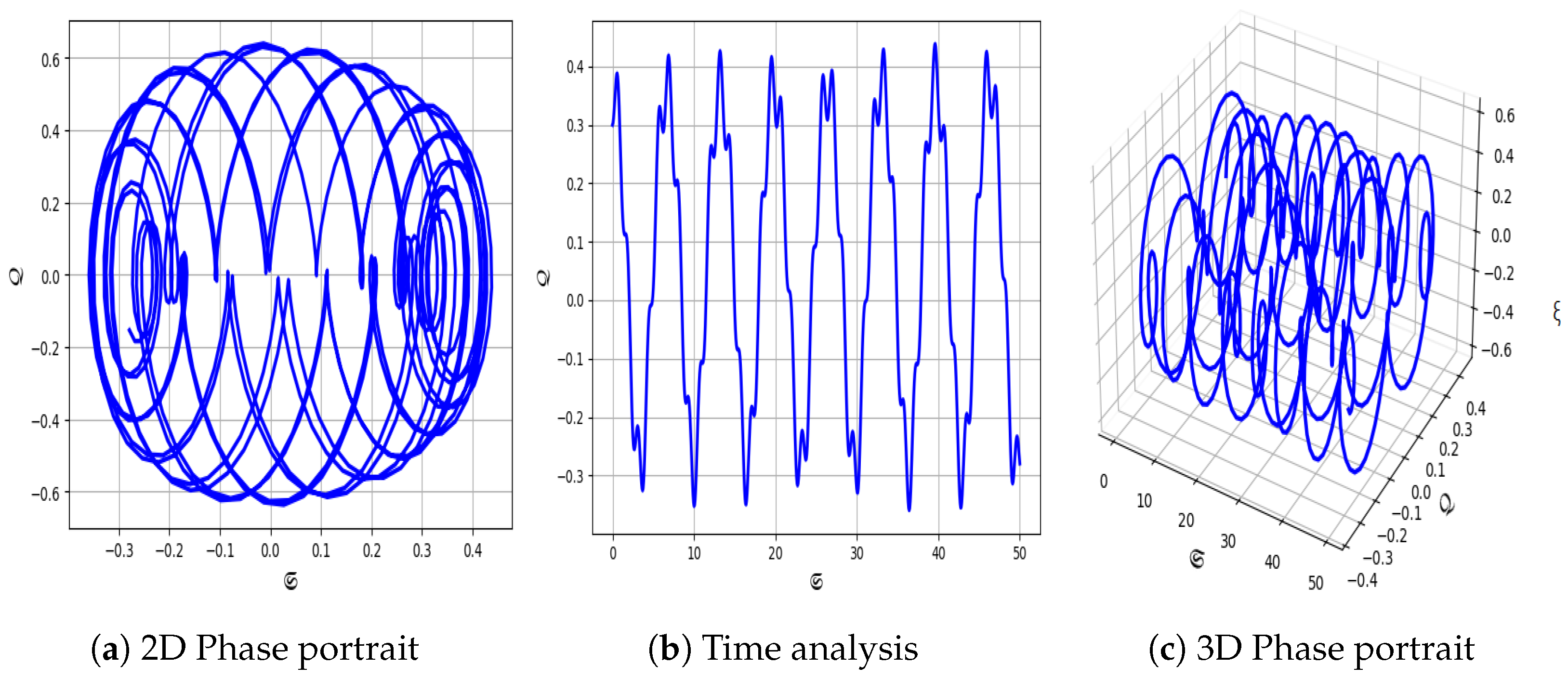
• In Figure 13, the system parameters are set to $\mathcal{G}=1.75$ and $\mu =2.1$ with $(\mathfrak{S},\mathcal{K})=(0.33,0.01)$, again demonstrating quasi-periodic behavior.
• In Figure 14, for $\mathcal{G}=3.75$ and $\mu =5.1$ with $(\mathfrak{S},\mathcal{K})=(0.33,0.01)$, the system continues to exhibit quasi-periodic behavior.
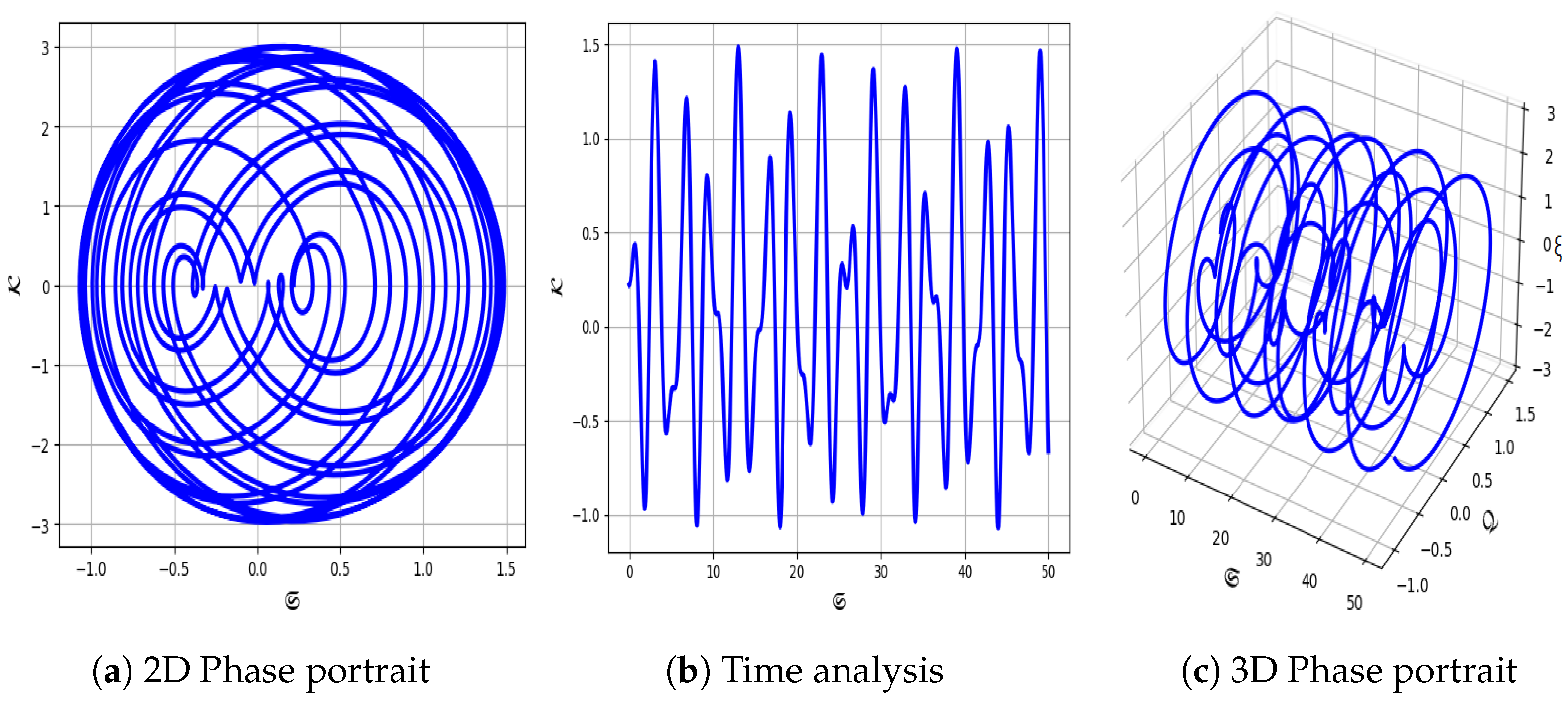
• In contrast, Figure 15 uses smaller values $\mathcal{G}=0.02$ and $\mu =0.01$ with initial conditions $(\mathfrak{S},\mathcal{K})=(0.55,0.01)$. For this configuration, the system displays clear periodic behavior.
• In Figure 16, we consider minimal values $\mathcal{G}=0.75$ and $\mu =3.4$ with initial conditions $(\mathfrak{S},\mathcal{K})=(0.45,0.01)$. Under these settings, the system exhibits quasi-periodic behavior.

6. Conclusions

In this study, we analyzed the dynamical behavior of a FNLWE in a MEEC rod, which has promising applications in materials science, smart structures, and advanced sensor systems. By incorporating geometric nonlinearity in the longitudinal direction and introducing an effective transverse Poisson’s ratio, we derived a nonlinear wave equation tailored for a long MEEC rod. We initially applied a fractional wave transformation to convert the FNLWE into a second-order nonlinear ordinary differential equation. Using the direct algebraic method, we obtained a spectrum of analytical solutions, each representing different types of nonlinear wave structures. The versatility and robustness of this method are reflected in the diversity of solutions derived. We further presented various graphical profiles, including 2D, 3D, and contour plots, to illustrate the physical behavior of the solutions under specific parameter regimes, as shown in Figure 1, Figure 2, Figure 3, Figure 4, Figure 5, Figure 6, Figure 7 and Figure 8. Figure 1 illustrates the 3D, 2D, and contour plots of the solution ${{\rm Y}}_1$, obtained using the parameters $\alpha =2$, $n=1$, $\phi =3$, $\vartheta =0.4$, $\rho =1.6$, $\omega =0.2$, $r=3$, $t=2$, $s=4$, $v=1$, and $\kappa =1.1$, under the condition $\Sigma ={\omega }^2-4\alpha \vartheta <0$ with $\alpha \ne 0$. Similarly, Figure 2 presents the solution ${{\rm Y}}_2$ using the same parameter values and condition. In Figure 3, the solution ${{\rm Y}}_6$ is plotted with the same parameters and condition. Figure 4 also employs the same parameter set and condition to depict ${{\rm Y}}_8$. In contrast, Figure 5 shows ${{\rm Y}}_8$ with parameters $\alpha =2$, $n=1$, $\phi =3$, $\vartheta =0.4$, $\rho =1.6$, $\omega =0$, $r=3$, $t=2$, $s=4$, $v=1$, $\kappa =1.1$, under the condition $\alpha \vartheta >0$ and $\omega =0$. Figure 6 also uses the same parameter values and conditions for plotting ${{\rm Y}}_8$. Figure 7 presents the solution ${{\rm Y}}_8$ using $\alpha =2$, $n=1$, $\phi =3$, $\vartheta =-0.4$, $\rho =1.6$, $\omega =0$, $r=3$, $t=2$, $s=4$, $v=1$, $\kappa =1.1$, under the condition $\alpha \vartheta <0$ and $\omega =0$. Lastly, Figure 8 illustrates ${{\rm Y}}_8$ with parameters $\alpha =-0.4$, $n=1$, $\phi =3$, $\vartheta =0.4$, $\rho =1.6$, $\omega =0.2$, $r=3$, $t=2$, $s=4$, $v=1$, $\kappa =1.1$, under the condition $\omega =0$, $\alpha =-\vartheta$, and $\alpha \ne 0$.

Moreover, we qualitatively explored quasi-periodic dynamics and sensitivity behavior by transforming the wave equation into a dynamical system using the Galilean transformation. Through sensitivity analysis under varying initial conditions as shown in Figure 9, Figure 10, Figure 11 and Figure 12, we observed that the system exhibits high sensitivity to perturbations. To delve deeper into complex dynamics, a perturbation term $\mathcal{G}\cos \left(\mu \xi \right)$ was introduced into the system (17), facilitating the analysis of chaotic behavior. These dynamics were further illustrated using phase portraits, time series, 2D, and 3D plots for different values of $\mathcal{G}$ and $\mu$ as shown in Figure 13, Figure 14, Figure 15 and Figure 16, revealing quasi-periodic structures.

Potential applications of the presented results include the design and control of wave propagation in advanced functional materials, development of high-precision sensors, and modeling of nonlinear phenomena in piezoelectric and magneto-electro-elastic systems. The exact wave solutions and the sensitivity insights provided in this work can serve as a theoretical foundation for engineering devices where tailored wave dynamics are essential. For future work, this model can be extended through symmetry analysis and the derivation of conservation laws. Additionally, more complex wave structures such as lump, breather, and rogue wave solutions could be investigated using alternative analytical approaches like the Hirota bilinear method, Lie group analysis, and variational techniques. Incorporating stochastic or higher-order effects may also offer a broader understanding of real-world applications in smart material modeling and nonlinear signal transmission.

References

1. Murad, M.A.S.; Ismael, H.F.; Sulaiman, T.A. Various exact solutions to the time-fractional nonlinear Schrödinger equation via the new modified Sardar sub-equation method. Phys. Scr. 2024, 99, 085252. [Google Scholar] [CrossRef]
2. Wazwaz, A.M. Breather wave solutions for an integrable (3+1)-dimensional combined pKP–BKP equation. Chaos Solitons Fractals 2024, 182, 114886. [Google Scholar] [CrossRef]
3. Wang, K.L.; Wei, C.F. Novel optical soliton solutions of the fractional perturbed Schrödinger equation in optical fiber. Fractals 2024, 33, 2450147. [Google Scholar] [CrossRef]
4. Cattani, C.; Sulaiman, T.A.; Baskonus, H.M.; Bulut, H. Solitons in an inhomogeneous Murnaghan’s rod. Eur. Phys. J. Plus 2018, 133, 228. [Google Scholar] [CrossRef]
5. Muhammad, J.; Younas, U.; Hussain, E.; Ali, Q.; Sediqmal, M.; Kedzia, K.; Jan, A.Z. Solitary wave solutions and sensitivity analysis to the space-time β-fractional Pochhammer–Chree equation in elastic medium. Sci. Rep. 2024, 14, 28383. [Google Scholar] [CrossRef]
6. Younas, U.; Hussain, E.; Muhammad, J.; Sharaf, M.; Meligy, M.E. Chaotic Structure, Sensitivity Analysis and Dynamics of Solitons to the Nonlinear Fractional Longitudinal Wave Equation. Int. J. Theor. Phys. 2025, 64, 42. [Google Scholar] [CrossRef]
7. Younas, U.; Hussain, E.; Muhammad, J.; Garayev, M.; El-Meligy, M. Bifurcation analysis, chaotic behavior, sensitivity demonstration and dynamics of fractional solitary waves to nonlinear dynamical system. Ain Shams Eng. J. 2025, 16, 103242. [Google Scholar] [CrossRef]
8. Malik, S.; Hashemi, M.S.; Kumar, S.; Rezazadeh, H.; Mahmoud, W.; Osman, M.S. Application of new Kudryashov method to various nonlinear partial differential equations. Opt. Quantum Electron. 2023, 55, 8. [Google Scholar] [CrossRef]
9. Malik, S.; Kumar, S.; Akbulut, A.; Rezazadeh, H. Some exact solitons to the (2 + 1)-dimensional Broer-Kaup-Kupershmidt system with two different methods. Opt. Quantum Electron. 2023, 55, 1215. [Google Scholar] [CrossRef]
10. Khatkar, A.; Shehla, F.; Sharma, A.; Kumar, S.; Yadav, R.; Malik, S. Nonlinear Shrödinger equation having self-phase modulation without chromatic dispersion: Sensitivity analysis and novel soliton solutions. Nonlinear Dyn. 2025, 113, 13681–13697. [Google Scholar] [CrossRef]
11. Zayed, E.M.; Alurrfi, K.A.; Hasek, A.M.; Arnous, A.H.; Secer, A.; Ozisik, M.; Kumar, S. Perturbations of optical solitons in magneto-optic waveguides incorporating multiplicative white noise and sixth-order dispersion: A study of the Sasa-Satsuma equation. Pramana 2025, 99, 22. [Google Scholar] [CrossRef]
12. Kumar, S.; Malik, S. A new analytic approach and its application to new generalized Korteweg-de Vries and modified Korteweg-de Vries equations. Math. Methods Appl. Sci. 2024, 47, 11709–11726. [Google Scholar] [CrossRef]
13. Bhan, C.; Karwasra, R.; Malik, S.; Kumar, S. Bifurcation, chaotic behavior and soliton solutions to the KP-BBM equation through new Kudryashov and generalized Arnous methods. AIMS Math. 2024, 9, 8749–8767. [Google Scholar] [CrossRef]
14. Qu, H.D.; Liu, X.; Lu, X.; ur Rahman, M.; She, Z.H. Neural network method for solving nonlinear fractional advection-diffusion equation with spatiotemporal variable-order. Chaos Solitons Fractals 2022, 156, 111856. [Google Scholar] [CrossRef]
15. Wu, X.S.; Liu, J.G. Solving the variable coefficient nonlinear partial differential equations based on the bilinear residual network method. Nonlinear Dyn. 2024, 112, 8329–8340. [Google Scholar] [CrossRef]
16. Waseem; Yun, W.; Boulaaras, S.; ur Rahman, M. Exploring hybrid Sisko nanofluid on a stretching sheet: An improved cuckoo search-based machine learning approach. Eur. Phys. J. Plus 2024, 139, 760. [Google Scholar] [CrossRef]
17. Xue, C.X.; Pan, E.; Zhang, S.Y. Solitary waves in a magneto-electro-elastic circular rod. Smart Mater. Struct. 2011, 20, 105010. [Google Scholar] [CrossRef]
18. Roshid, M.M.; Uddin, M.; Hossain, M.M. Investigation of rogue wave and dynamic solitary wave propagations of the M-fractional (1+1)-dimensional longitudinal wave equation in a magnetic-electro-elastic circular rod. Indian J. Phys. 2025, 99, 1787–1803. [Google Scholar] [CrossRef]
19. Djaouti, A.M.; Roshid, M.M.; Abdeljabbar, A.; Al-Quran, A. Bifurcation analysis and solitary wave solution of fractional longitudinal wave equation in magneto-electro-elastic (MEE) circular rod. Results Phys. 2024, 64, 107918. [Google Scholar] [CrossRef]
20. Kumar, A.; Kumar, S.; Bohra, N.; Pillai, G.; Kapoor, R.; Rao, J. Exploring soliton solutions and interesting wave-form patterns of the (1+1)-dimensional longitudinal wave equation in a magnetic-electro-elastic circular rod. Opt. Quantum Electron. 2024, 56, 1029. [Google Scholar] [CrossRef]
21. Li, B.; Liang, H.; He, Q. Multiple and generic bifurcation analysis of a discrete Hindmarsh-Rose model. Chaos Solitons Fractals 2021, 146, 110856. [Google Scholar] [CrossRef]
22. Zhang, X.; Yang, X.; He, Q. Multi-scale systemic risk and spillover networks of commodity markets in the bullish and bearish regimes. N. Am. J. Econ. Financ. 2022, 62, 101766. [Google Scholar] [CrossRef]
23. Zhu, X.; Xia, P.; He, Q.; Ni, Z.; Ni, L. Coke price prediction approach based on dense GRU and opposition-based learning salp swarm algorithm. Int. J. Bio-Inspired Comput. 2023, 21, 106–121. [Google Scholar] [CrossRef]
24. Eskandari, Z.; Avazzadeh, Z.; Khoshsiar Ghaziani, R.; Li, B. Dynamics and bifurcations of a discrete-time Lotka-Volterra model using nonstandard finite difference discretization method. Math. Methods Appl. Sci. 2022, 48, 7197–7212. [Google Scholar] [CrossRef]
25. Borhan, J.R.M.; Mamun Miah, M.; Duraihem, F.Z.; Iqbal, M.A.; Ma, W.X. New optical soliton structures, bifurcation properties, chaotic phenomena, and sensitivity analysis of two nonlinear partial differential equations. Int. J. Theor. Phys. 2024, 63, 183. [Google Scholar] [CrossRef]
26. Li, Z.; Lyu, J.; Hussain, E. Bifurcation, chaotic behaviors and solitary wave solutions for the fractional Twin-Core couplers with Kerr law non-linearity. Sci. Rep. 2024, 14, 22616. [Google Scholar] [CrossRef]
27. Shah, S.A.A.; Hussain, E.; Ma, W.X.; Li, Z.; Ragab, A.E.; Khalaf, T.M. Qualitative analysis and new variety of solitons profiles for the (1+1)-dimensional modified equal width equation. Chaos Solitons Fractals 2024, 187, 115353. [Google Scholar] [CrossRef]
28. Hussain, E.; Li, Z.; Shah, S.A.A.; Az-Zo’bi, E.A.; Hussien, M. Dynamics study of stability analysis, sensitivity insights and precise soliton solutions of the nonlinear (STO)-Burger equation. Opt. Quantum Electron. 2023, 55, 1274. [Google Scholar] [CrossRef]
29. Almusawa, H.; Jhangeer, A. Soliton solutions, Lie symmetry analysis and conservation laws of ionic waves traveling through microtubules in live cells. Results Phys. 2022, 43, 106028. [Google Scholar] [CrossRef]
30. Samreen, M. Exploring quasi-periodic behavior, bifurcation, and traveling wave solutions in the double-chain DNA model. Chaos Solitons Fractals 2025, 192, 116052. [Google Scholar] [CrossRef]
31. Ali, K.K.; Faridi, W.A.; Tarla, S. Phase trajectories and Chaos theory for dynamical demonstration and explicit propagating wave formation. Chaos Solitons Fractals 2024, 182, 114766. [Google Scholar] [CrossRef]
32. Ali, K.K. Kudryashov-Sinelshchikov equation: Phase portraits, bifurcation analysis and solitary waves. Opt. Quantum Electron. 2024, 56, 1627. [Google Scholar] [CrossRef]
Figure 1. Graphical profiles of Υ 1 ( x , t ) for different fractional orders of Ψ ( ξ ) . Parameters: α = 2 , n = 1 , φ = 3 , ϑ = 0.4 , ρ = 1.6 , ω = 0.2 , r = 3 , t = 2 , s = 4 , v = 1 , κ = 1.1 .
Fractalfract 09 00309 g001
Figure 2. Graphical profiles of Υ 1 ( x , t ) for different fractional orders of Ψ ( ξ ) with α = 2 , n = 1 , φ = 3 , ϑ = 0.4 , ρ = 1.6 , ω = 0.2 , r = 3 , t = 2 , s = 4 , v = 1 , κ = 1.1 .
Fractalfract 09 00309 g002
Figure 3. Graphical profiles of Υ 6 ( x , t ) for different fractional orders of Ψ ( ξ ) with α = 2 , n = 1 , φ = 3 , ϑ = 0.4 , ρ = 1.6 , ω = 0.2 , r = 3 , t = 2 , s = 4 , v = 1 , and κ = 1.1 .
Fractalfract 09 00309 g003
Figure 4. Graphical profiles of Υ 8 ( x , t ) for different fractional orders of Ψ ( ξ ) with α = 2 , n = 1 , φ = 3 , ϑ = 0.4 , ρ = 1.6 , ω = 0.2 , r = 3 , t = 2 , s = 4 , v = 1 , and κ = 1.1 .
Fractalfract 09 00309 g004
Figure 5. Graphical profiles of Υ 11 ( x , t ) for different fractional orders of Ψ ( ξ ) with α = 2 , n = 1 , φ = 3 , ϑ = 0.4 , ρ = 1.6 , ω = 0 , r = 3 , t = 2 , s = 4 , v = 1 , and κ = 1.1 .
Fractalfract 09 00309 g005
Figure 6. Graphical profiles of Υ 15 ( x , t ) for different fractional orders of Ψ ( ξ ) with α = 2 , n = 1 , φ = 3 , ϑ = 0.4 , ρ = 1.6 , ω = 0 , r = 3 , t = 2 , s = 4 , v = 1 , and κ = 1.1 .
Fractalfract 09 00309 g006
Figure 7. Graphical profiles of Υ 15 ( x , t ) for different fractional orders of Ψ ( ξ ) with α = 2 , n = 1 , φ = 3 , ϑ = 0.4 , ρ = 1.6 , ω = 0 , r = 3 , t = 2 , s = 4 , v = 1 , and κ = 1.1 .
Fractalfract 09 00309 g007
Figure 8. Graphical profiles of Υ 15 ( x , t ) for different fractional orders of Ψ ( ξ ) with α = 0.4 , n = 1 , φ = 3 , ϑ = 0.4 , ρ = 1.6 , ω = 0 , r = 3 , t = 2 , s = 4 , v = 1 , and κ = 1.1 .
Fractalfract 09 00309 g008
Figure 9. Exploring sensitivity analysis in system (17) with ( 0.01 , 0.01 ) and ( 0.02 , 0.01 ) .
Fractalfract 09 00309 g009
Figure 10. Exploring sensitivity analysis in system (17) with ( 0.01 , 0.01 ) and ( 0.04 , 0.01 ) .
Fractalfract 09 00309 g010
Figure 11. Exploring sensitivity analysis in system (17) with ( 0.01 , 0.01 ) and ( 0.09 , 0.01 ) .
Fractalfract 09 00309 g011
Figure 12. Exploring sensitivity analysis in system (17) with ( 0.01 , 0.01 ) , ( 0.04 , 0.01 ) , and ( 0.09 , 0.01 ) .
Fractalfract 09 00309 g012
Figure 13. Quasi-periodic behavior of system (18) with G = 0.75 , μ = 3.4 , and initial conditions ( S , J ) = ( 0.45 , 0.01 ) .
Fractalfract 09 00309 g013
Figure 14. Quasi-periodic behavior of system (18) with G = 1.75 , μ = 2.1 , and initial conditions ( S , J ) = ( 0.33 , 0.01 ) .
Fractalfract 09 00309 g014
Figure 15. Quasi-periodic behavior of system (18) with G = 3.75 , μ = 5.1 , and initial conditions ( S , J ) = ( 0.33 , 0.01 ) .
Fractalfract 09 00309 g015
Figure 16. Periodic behavior of system (18) with G = 0.02 , μ = 0.01 , and initial conditions ( S , J ) = ( 0.55 , 0.01 ) .
Fractalfract 09 00309 g016
Disclaimer/Publisher’s Note: The statements, opinions and data contained in all publications are solely those of the individual author(s) and contributor(s) and not of MDPI and/or the editor(s). MDPI and/or the editor(s) disclaim responsibility for any injury to people or property resulting from any ideas, methods, instructions or products referred to in the content.