Abstract
This study proposes a novel image segmentation method, MF-DFA combined with the Allen–Cahn equation (MF-AC-DFA). By utilizing the Allen–Cahn equation instead of the least squares method employed in traditional MF-DFA for fitting, the accuracy and robustness of image segmentation are significantly improved. The article first conducts segmentation experiments under various conditions, including different target shapes, image backgrounds, and resolutions, to verify the feasibility of MF-AC-DFA. It then compares the proposed method with gradient segmentation methods and demonstrates the superiority of MF-AC-DFA. Finally, real-life wire diagrams and transmission tower diagrams are used for segmentation, which shows the application potential of MF-AC-DFA in complex scenes. This method is expected to be applied to the real-time state monitoring and analysis of power facilities, and it is anticipated to improve the safety and reliability of the power grid.
1. Introduction
Electric power infrastructure is crucial for societal and industrial stability. Transmission towers, as key components of the power system, ensure the safe and stable operation of power lines and have been extensively studied by scholars. The increasing global demand for electricity highlights the critical nature of transmission line construction and maintenance. Transmission towers, due to their tall and flexible structures, are particularly vulnerable to wind-induced vibrations, as shown by Roy and Kundu []. These vibrations can cause fatigue damage, potential collapse, and significant consequences. Therefore, analyzing and mitigating wind-induced vibrations in transmission towers is crucial for ensuring power system safety and minimizing disaster losses. Tian et al. [] studied the ultimate load capacity and failure mechanisms of lattice-type steel tube transmission towers under extreme wind loads. Using full-scale tests and finite element simulations, they analyzed structural response, capacity, and failure modes, focusing on buckling and softening behavior. Their model accurately replicated experimental observations of displacement, load capacity, and failure characteristics. Wang et al. [] investigated the effect of temperature on transmission tower inclination. Using the MF-DCCA method, they analyzed the cross-correlation between sensor temperature and tower tilt, and they validated the relationship with Pearson’s coefficient and linear fitting. Their study revealed multifractal characteristics in the time series, indicating potential improvements for grid safety and reliability in cold regions.
However, due to aging infrastructure and environmental impacts, regular monitoring and maintenance of transmission towers are crucial for ensuring the safety and reliability of the power system. Traditionally, power line and transmission tower monitoring has relied on manual inspections and increasingly popular drone patrols. Although these methods ensure operational safety, they also encounter various challenges. With advancements in science and technology, image processing has been applied to the automatic identification and analysis of power facility conditions. Utilizing advanced image segmentation techniques, researchers can more accurately detect changes in the state of power lines and transmission towers. Damodaran et al. [] proposed a machine learning-based image segmentation method for recognizing high-altitude transmission lines, utilizing a graphics processor for accelerated computation. The method, trained on preprocessed UAV images and multiple classification models, showed that the extreme gradient boosting algorithm was optimal in terms of accuracy and predictive performance. In contrast, Ma et al. [] employed instance segmentation to simultaneously detect transmission towers and lines. Resolving challenges posed by large, high-resolution aerial images with low signal-to-noise ratio and high aspect ratio, they improved the SOLOv2 network for instance segmentation. Comparative experiments demonstrated higher segmentation accuracy with the improved network. He et al. [] introduced TLSUNet, an enhanced UNet segmentation model that reduces computational complexity and the number of parameters while improving segmentation performance. This was achieved by incorporating a lightweight backbone network and a hybrid feature extraction module. Experimental results on aerial photography datasets indicated higher mIOU and mDice metrics, and this offered new approaches for image segmentation in complex, resource-constrained scenarios.
Multifractal detrended fluctuation analysis (MF-DFA) is an algorithm utilized to analyze the long-range correlation of time series and their complex fluctuation characteristics. MF-DFA is based on the traditional Detrended Fluctuation Analysis (DFA). In one dimension, MF-DFA has been commonly utilized in several fields [,,]. The MF-DFA method effectively analyzes image complexity and self-similarity. Wang et al. [] proposed the MF-LSSVM-DFA model, addressing overfitting/underfitting issues in traditional MF-DFA by employing LSSVM instead of fixed-order polynomial fitting and thereby improving accuracy and adaptability. The study validated the model using a multiplicative cascade time series and applied it to medical fields like ECG signal classification, showing its accuracy and robustness. Yue et al. [] introduced a 2D MF-DFA method for singularity detection in substation equipment infrared images. It computes the generalized Hurst index per pixel, uses it for box-counting dimension calculation, and extracts image edges. Results indicate effective segmentation of equipment regions in infrared images of varying complexity. The literature [] highlights MF-DFA’s superior performance in noisy environments. However, in the traditional MF-DFA method, the least squares method is usually used for linear fitting to eliminate the trend component in the data, so as to ensure the accuracy of the analysis results []. However, linear fitting is only suitable for simple trends and cannot handle complex non-linear trends. When dealing with complex sequences, linear fitting may lead to incomplete trend removal [].
The Allen–Cahn (AC) equation, as a classical nonlinear partial differential equation, has played an important role in describing phase transition and interface evolution problems since it was proposed by Allen and Cahn in 1979 []. The AC equation, as an important nonlinear partial differential equation, has shown significant advantages in simulating interface evolution and complex system dynamics []. Through the study of linear implicit methods, it is proved that the AC equation can efficiently and stably handle interface evolution problems after combining small positive parameters and nonlinear terms. In addition, the AC equation with spatial-dependent migration rates and nonlinear diffusion are discussed separately [,], and this discussion reveals the crucial role of nonlinear terms in describing the dynamics of particle systems and the evolution of complex geometric interfaces. Compared with other nonlinear equations such as the Navier–Stokes equation and the Cahn–Hilliard (CH) equation [], the AC equation can efficiently handle dynamic geometric interface problems by introducing order parameters. It was verified to be efficient and stable in the evolution of 1D and 2D interfaces, and the advantages of its nonlinear terms in describing the evolution of complex geometric shapes were pointed out [,]. The application of the AC equation in multiphase flow and non-conservative systems was discussed, and its flexibility and accuracy, in comparison with the CH equation [], were emphasized. In summary, the AC equation has significant advantages over other nonlinear equations in terms of interface evolution, numerical stability, and adaptability of nonlinear terms [].
Therefore, we proposed to introduce the AC equation into the MF-DFA for the detrending step, so as to improve the accuracy and reliability of image segmentation. Currently, there are relatively few studies combining the MF-DFA method with the AC equation for power transmission tower image segmentation. This paper aims to investigate the potential application of this combination method in image segmentation. Through a series of experiments, the effectiveness of the proposed algorithm is verified, and finally, its advantages in processing complex real images, such as transmission tower images, are demonstrated.
2. Methodology
Now, we propose a method for image segmentation using multifractal detrended fluctuation analysis (MF-DFA) combined with the AC equation (MF-AC-DFA), which improves and extends traditional multifractal detrended fluctuation analysis. In this section, we present our proposed method in two subsections.
2.1. Allen–Cahn Equation
The AC equation is a mathematical model used to simulate phase transition processes, the evolution of interfaces towards equilibrium, and image segmentation []. The differential equation can be expressed as:
where is the partial derivative of u with respect to time t. It describes how the quantity u changes over time. Here, u refers to the solution in the AC equation; specifically, it represents the concentration distribution or phase field variables at different points in time and space. is a small parameter determining the width of the interfacial region. is the Laplacian operator, which describes the spatial second derivatives of u. It measures how u changes in space and is responsible for the smoothing effect in the equation. The term indicates diffusion, promoting smooth and flat boundaries between different phases, while is a nonlinear term driving the system towards one of two stable states: or . Intermediate states are unstable, which leads to the formation of sharp transition layers.
2.2. Two-Dimensional MF-AC-DFA
The methodology of MF-AC-DFA is similar to that of MF-DFA. The specific steps are as follows:
- Step 1.
- Read and preprocess the image by converting it to grayscale and double precision type for numerical operations.
- Step 2.
- Define parameters: window size for localization, half-width , and fractal dimension parameter q.
- Step 3.
- Extract and process sub-windows: for each pixel , extract a sub-window, partitioned into smaller chunks (s = 2 to ).
- Step 4.
- Combining the AC equation: For each small block of size , it is first transformed into a column vector , and then a function is called to transform in conjunction with the AC equation. Then, the transformed result is reshaped into the shape of the original nugget (), denoted as . Finally, the sum of squares of the errors before and after the processing of this nugget is calculated. The error sum of squares is calculated as follows:where denotes the pixel value of the original image block, which is an -sized image block, and denotes the reconstructed image block after fitting the transform by the AC equation. s represents the side length of the image block and is an inner loop control variable from 2 to , indicating the size of the currently processed sub-block.
- Step 5.
- The qth-order fluctuation function is computed by averaging over all the segments, that is:where and . and are the number of rows and columns inside the image block that can be sliced by step s, respectively. q controls the sensitivity to the error distribution. emphasizes large errors, emphasizes small errors, and corresponds to the mean square error.
- Step 6.
- Change the value of s within the range from 2 to , which governs the scaling characteristics of the fluctuation functions. These characteristics can be identified by examining the relationship between and for each given value of q. When the surfaces exhibit long-range power-law correlations, increases according to a power-law form as s becomes large:The is known as the generalized Hurst exponent. Note that A and B are not necessarily integer multiples of s, and the solution to this problem is the same as for MF-DFA: the same segmentation process can be repeated starting from the other three corners of the image.
2.3. Dice Coefficient
In this paper, the coefficient as a measure of segmentation results is used. The coefficient is a statistical tool for measuring the similarity of sets. It is widely used in the field of image processing and is especially useful in the evaluation of binarized segmentation results of regions. Its formula is as follows:
where X and Y represent two sample sets, respectively, X denotes the segmentation result outputted by the model, and Y denotes the real segmentation result manually labeled. denotes the intersection size of these two sets, i.e., the number of elements belonging to both set X and set Y. and are the numbers of elements in sets X and Y, respectively. The coefficient takes values between 0 and 1. If the two sets are identical, their coefficient is 1. If the two sets have no elements in common, their coefficient is 0. Therefore, the closer the coefficient is to 1, the higher the similarity between the two samples or sets.
All experiments in this study were conducted using MATLAB R2020a on an Intel® Core™ i5-13500H CPU, hosted on a HP computer, sourced from Palo Alto, CA, USA, with a 2.60 GHz processor.
3. Experiments Using MF-AC-DFA
This section presents a series of 2D spatial image segmentation experiments to validate the effectiveness of the proposed MF-AC-DFA algorithm in image segmentation applications. Before conducting the formal verification of the MF-AC-DFA segmentation effect experiment, some necessary experiments were carried out on the relevant parameters (see Section 2) to explain the method in more detail.
In Section 2.1, the parameter of the AC equation primarily controls the width of the interface. In Figure 1, the results of comparing the solution u of the equation with the original sequence for different values of are shown, and the effect of different values on the model is examined. Specifically, Figure 1a displays the numerical results of comparing u with the original sequence for , and Figure 1b shows the results of comparing u with the original for . The results show that the choice of value has a significant effect on the solution of the AC equation. A smaller value of will capture a steeper interface, while a larger value of will result in a smoother solution but may lose some fine structural features. Therefore, choosing the right value is important for the accuracy of the model.
Figure 1.
The variation in u for different numbers of when fixing iteration = 4. The original sequence is shown by the blue solid line, and u obtained for different values of is shown by the yellow circle. (a) is the comparison of with . (b) is the comparison of with .
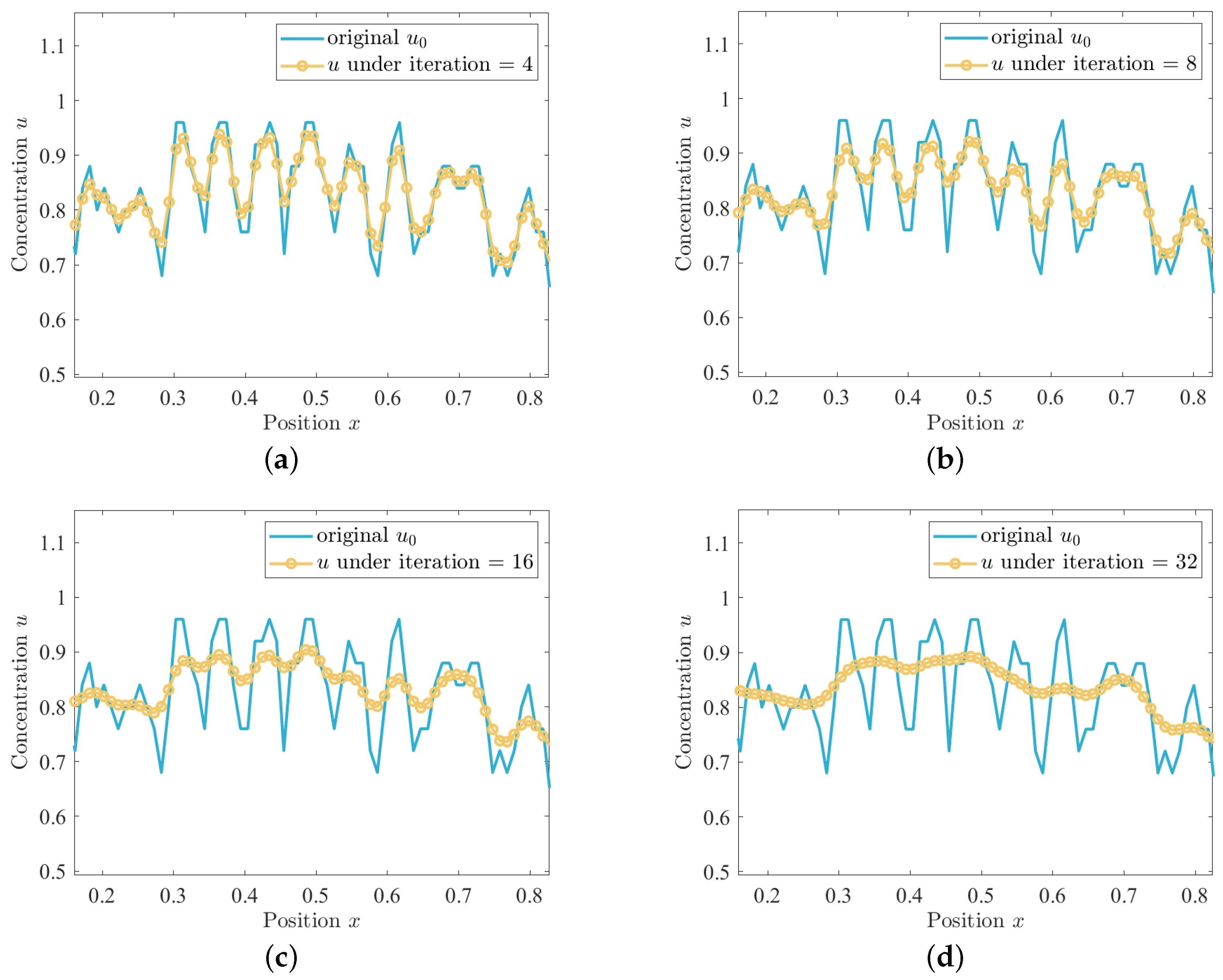
The significance of the number of iterations is in controlling the iterative process of the time step. Specifically, we update u incrementally by looping through multiple iterations to solve the partial differential equation. Each iteration corresponds to a time step, and through these iterations, we can observe how u changes over time. In Figure 2, the results of comparing the solution u of the equation with the original sequence for different numbers of iterations are shown. Specifically, Figure 2a–d show the results of comparing the solution u of the equation with the original sequence when the number of iterations is 4, 8, 16, and 32, respectively. When the number of iterations is reduced from 32 to 4, it can be seen that the solution of the equation is closer to the original sequence, which indicates that the choice of the number of iterations has a significant effect on the solution of the AC equation.
Figure 2.
The variation in u for different numbers of iterations when fixing = 0.1. The original sequence is shown by the blue solid line, and u obtained with different iteration numbers is shown by the yellow circle. (a) is the comparison of with an iteration number of 4. (b) is the comparison of with the number of iterations as 8. (c) is the comparison of with an iteration number of 16. (d) is the comparison of with an iteration number of 32.
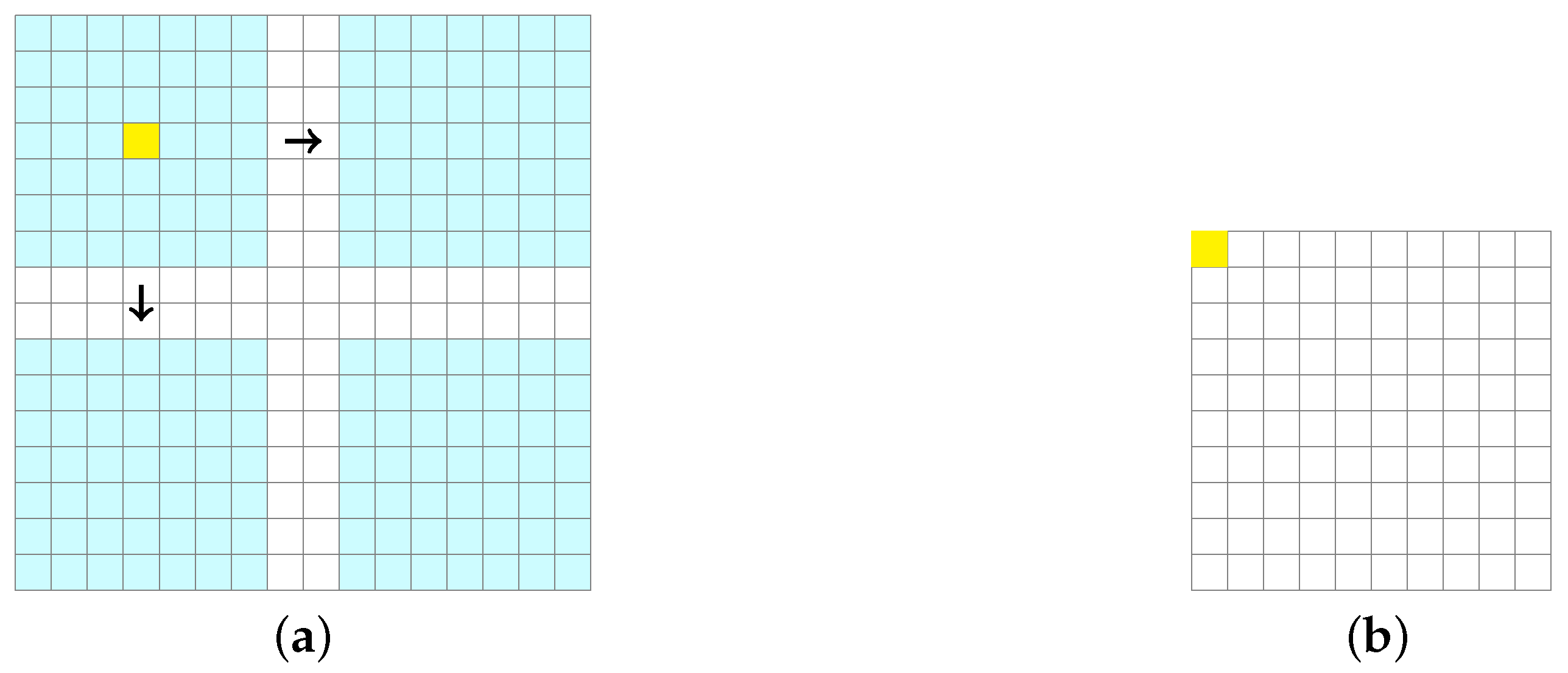
For the sliding window mentioned in Section 2.2, a legend is used here to explain the operation mechanism of the sliding window in detail, as shown in Figure 3. We process a pixel image with blue sliding windows, as shown in Figure 3a. To ensure that each window is completely inside the image, the center of the window starts at a position 3 pixels from the edge of the image (calculated from the half-width height ), starts at position (3, 3), and ends at the same position 3 pixels from the edge before it reaches the other side, up to position (12, 12). The blue sliding window in Figure 3a moves to the right and down in 1-pixel increments, covering the entire processable area. Since the space on each side is reduced by 3 pixels to ensure that the window falls entirely inside the image, the size of the processed image becomes pixels. The output image has pixels, as shown in Figure 3b, where each pixel value represents the result of the computation of a window at the corresponding position in the original image.
Figure 3.
A graphical representation of the sliding window algorithm. (a) The sliding window moves the process to the right and down on the original image. (b) The final output image.
The choice of the fractal dimension q is also essential when using the proposed method for image segmentation. A range of q values are explored, as shown in Figure 4. Figure 4a is the original image, and Figure 4b–f are the segmentation effects under different values of q, respectively. By comparison, our method with different q values shows significant differences in image segmentation effects. Specifically, Figure 4b–d, with q values of −5, −2, −1, and 1, respectively, show that the edge detection is not clear enough and the boundaries of some regions are blurred. Figure 4f, with , shows the clearest edge detection results, with well-defined boundaries of individual shapes and no obvious noise interference, while maintaining the detailed information of the image. Therefore, it can be concluded that the method has the best image segmentation effect when and can capture the boundary information of the target region more accurately. In the following experiments, the window size is set to 7 and q is set to 5, unchanged, unless otherwise noted.
Figure 4.
Image segmentation at different q values. (a) is original image. (b) is when . (c) is when . (d) is when . (e) is when . (f) is when .
3.1. Feasibility Experiments of MF-AC-DFA
This subsection demonstrates the feasibility of the proposed method by altering the geometry’s shape, the image’s background color, and its resolution.
First, three geometric shapes (circle, triangle, square) are drawn on the same background, each with a resolution of , as shown in Figure 5a–c. The best segmentation results for the three shapes are shown in Figure 5d–f, which demonstrates complete segmentation for each shape. Table 1 lists the specific coefficient values. The coefficients for circle, triangle, and square images are 0.9853, 0.9524, and 0.9696, respectively. These values, near 1, indicate segmentation results close to reality with minor variations. The algorithm demonstrates stability across the three shapes but exhibits varying sensitivity to each shape.
Figure 5.
The image segmentation of different geometries. The original images of (a) a circle, (b) a triangle, and (c) a square. The segmented images of (d) a circle, (e) a triangle, and (f) a square.
Table 1.
coefficient for different graphics.
Next, the proposed algorithm’s performance under different color backgrounds is evaluated using three images with red, green, and blue backgrounds, as shown in Figure 6a–c. The best segmentation results are shown in Figure 6d–f. Visually, the segmentation results are very close to the original graphs, which indicates that the algorithm can effectively separate black circular targets from backgrounds of various colors. Table 2 provides a more specific quantitative evaluation. For the red background, the coefficient is 0.9815, for the green background, the coefficient is 0.9803, and for the blue background, the coefficient is also 0.9803. These values are all very close to 1, which implies that the segmentation results are highly consistent with the real situation and proves that the algorithm is highly accurate and stable in dealing with these three background colors.
Figure 6.
The image segmentation of the same graphic with three different color backgrounds. The original image on a (a) red background, (b) green background, and (c) blue background. The segmented image on a (d) red background, (e) green background, and (f) blue background.
Table 2.
The coefficient for three background colors in the same graphics.
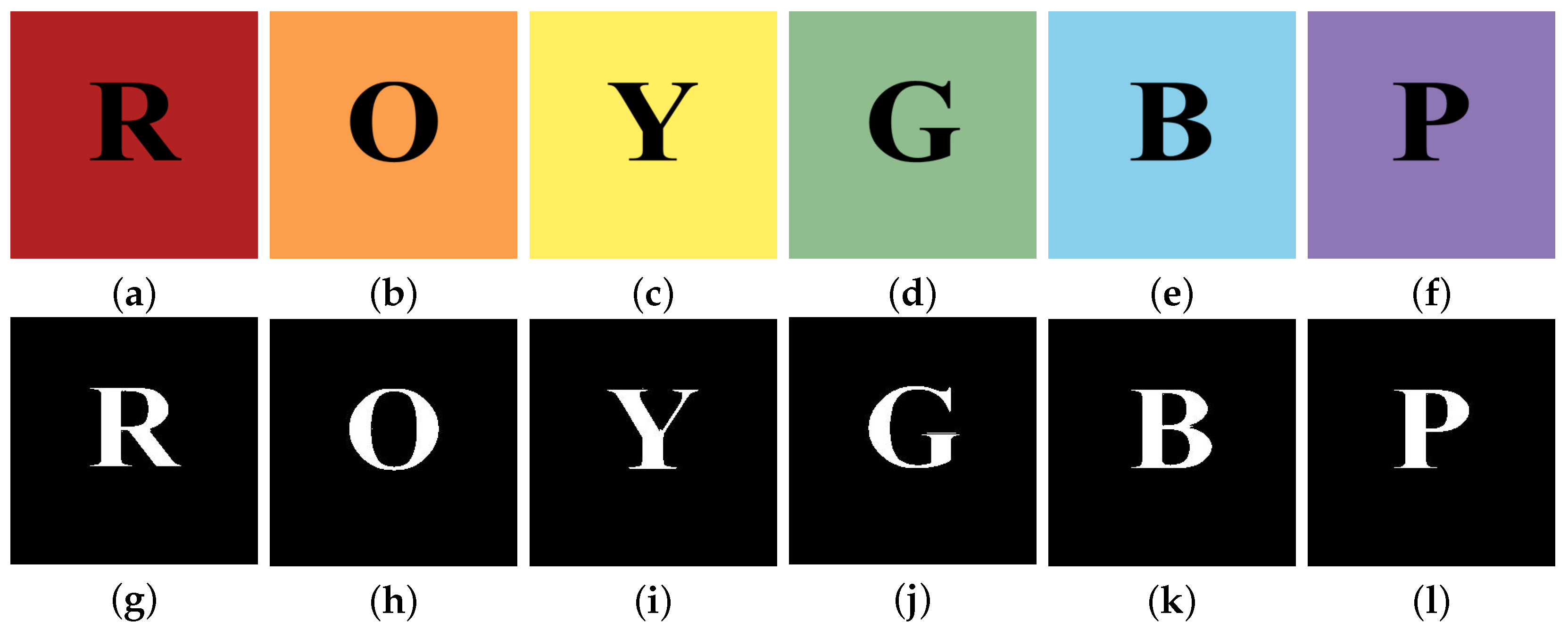
Further, six background images with varying colors and different English letters are selected for further testing. Figure 7a–f show the different background colors, which are red, orange, yellow, green, blue, and purple. They all have a resolution of . Optimal segmentation results, achieved by adjusting constraints, are presented in Figure 7g–l. Visually, the English letters are segmented effectively, irrespective of the background color. From the qualitative point of view, according to Table 3, the coefficients are 0.9677 for the red background, 0.9630 for the orange background, 0.9593 for the yellow background, 0.9365 for the green background, and 0.9671 for the blue background, and the highest value of 0.9728 is reached for the purple background. These values show that the algorithm can effectively and accurately segment the target from different color backgrounds. Except for the green background containing the letter G, all other background colors have a dice coefficient of about 0.96. This further proves that the proposed algorithm is still effective with different-colored backgrounds. However, the algorithm is more sensitive to different target shapes.
Figure 7.
Image segmentation for different graphics with different six color backgrounds. Original image on (a) red background, (b) orange background, (c) yellow background, (d) green background, (e) blue background, and (f) purple background. Segmented image on (g) red background, (h) orange background, (i) yellow background, (j) green background, (k) blue background, and (l) purple background.
Table 3.
coefficient at different graphics with six different color backgrounds.
Finally, consider whether our proposed algorithm is feasible on images with different resolutions. The red, green, and blue background images from the previous experiment were used; see Figure 8a,e,i. Then, three different resolutions were chosen for the experiment. Figure 8b,f,j are all images with resolution, Figure 8c,g,k are all images with resolution, and Figure 8d,h,l are all images with resolution. Visually, the match between the segmentation result and the original graphic increases gradually as the resolution increases, especially at the highest resolution of , where the segmentation effect is most ideal. Querying Table 4 gives the coefficients for different background colors at different resolutions. For the red background, the coefficient is 0.8633 when the resolution is ; when the resolution is , the coefficient is elevated to 0.9443; and the coefficient reaches the highest 0.9677 at the resolution of . Similarly, for the green background, the coefficients are 0.8358, 0.8930, and 0.9365, while for the blue background, the coefficients are 0.9137, 0.9341, and 0.9671, respectively. These values indicate that the segmentation accuracy increases significantly with increasing resolution and shows this trend for all three background colors.
Figure 8.
Image segmentation at different resolutions. Original image on (a) red background, (e) green background, and (i) blue background. Segmented image on (b) red background, (f) green background, and (j) blue background at resolution. Segmented image on (c) red background, (g) green background, and (k) blue background at resolution. Segmented image on (d) red background, (h) green background, and (l) blue background at resolution.
Table 4.
coefficient at different resolutions.
Overall, the proposed segmentation algorithm is not only robust to background color changes and target shape changes but also well adapted to changes in image resolution. Although the segmentation effect is slightly inferior at lower resolutions, the algorithm can achieve more accurate segmentation as the resolution increases. Therefore, the proposed segmentation method is widely feasible.
3.2. Superiority Experiments of MF-AC-DFA
In this subsection, the differences between the proposed MF-AC-DFA method and the gradient method for image segmentation are compared through a series of experiments.
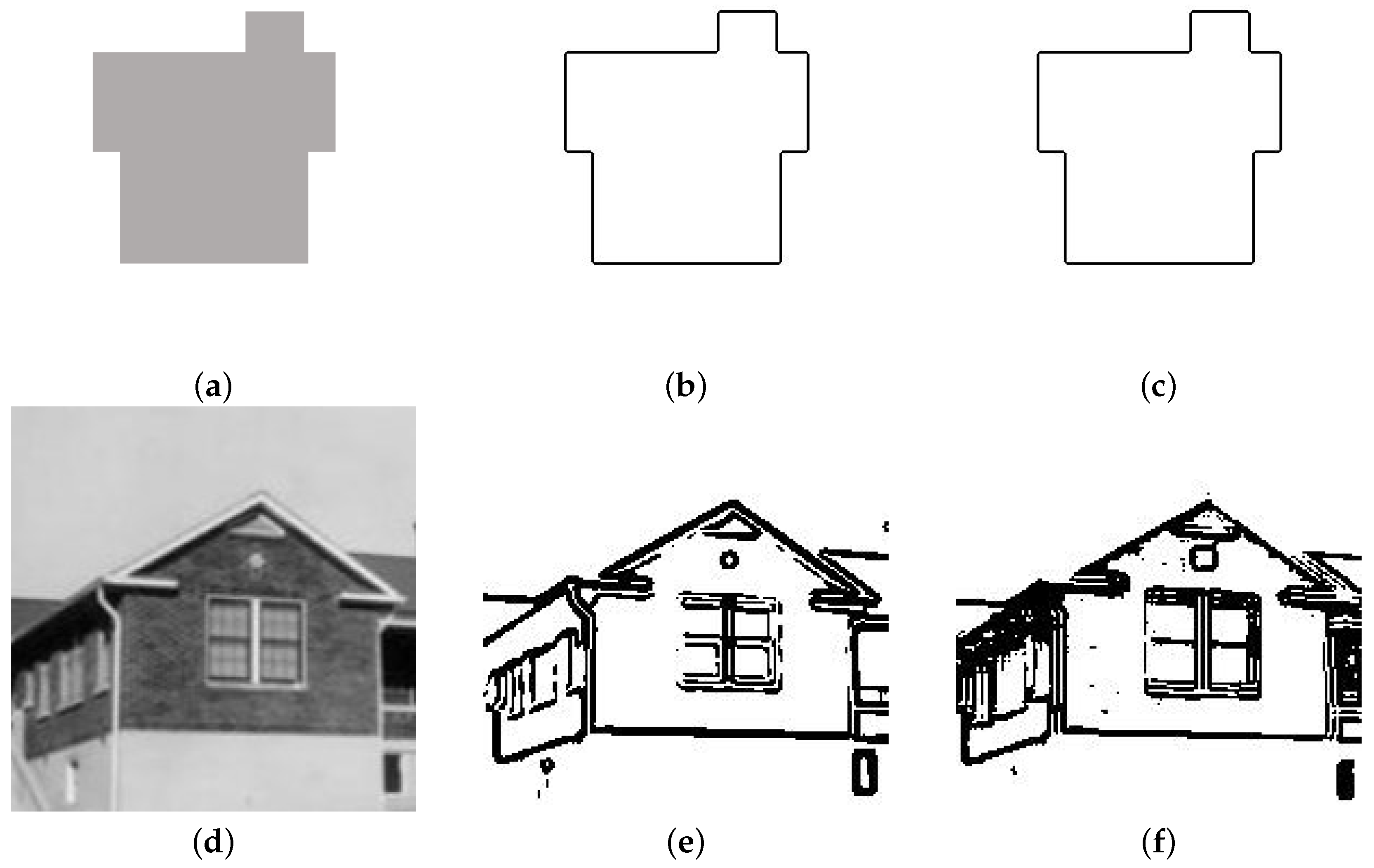
Figure 9 shows the comparison results of the two segmentation algorithms in geometric and real scenes. Specifically, Figure 9a shows a geometric house image and Figure 9d shows a real house image. To evaluate the performance of the different methods, this experiment applied the gradient method and the MF-AC-DFA method for segmentation, respectively. The computational results are displayed in Figure 9b,c,e,f. For geometric house images, no matter which method is used, good contour results are obtained, as shown in Figure 9b,c. In the segmentation experiments of real house images, by comparing Figure 9e,f, it can be seen that the gradient method does not perform as satisfactorily as using MF-AC-DFA. Since the real scene contains more complex details and noise, the gradient method is easily disturbed during the segmentation process, which results in a lack of clarity of the segmentation boundary and the phenomenon of missing information in some regions. The MF-AC-DFA method, on the other hand, can obtain the details of the house effectively and shows stronger accuracy.
Figure 9.
Comparison of two segmentation algorithms in geometric and real scenes. (a) Geometric house image. (b) Result of (a) using gradient method. (c) Result of (a) using MF-AC-DFA. (d) Real house image. (e) Result of (d) using gradient method. (f) Result of (d) using MF-AC-DFA.
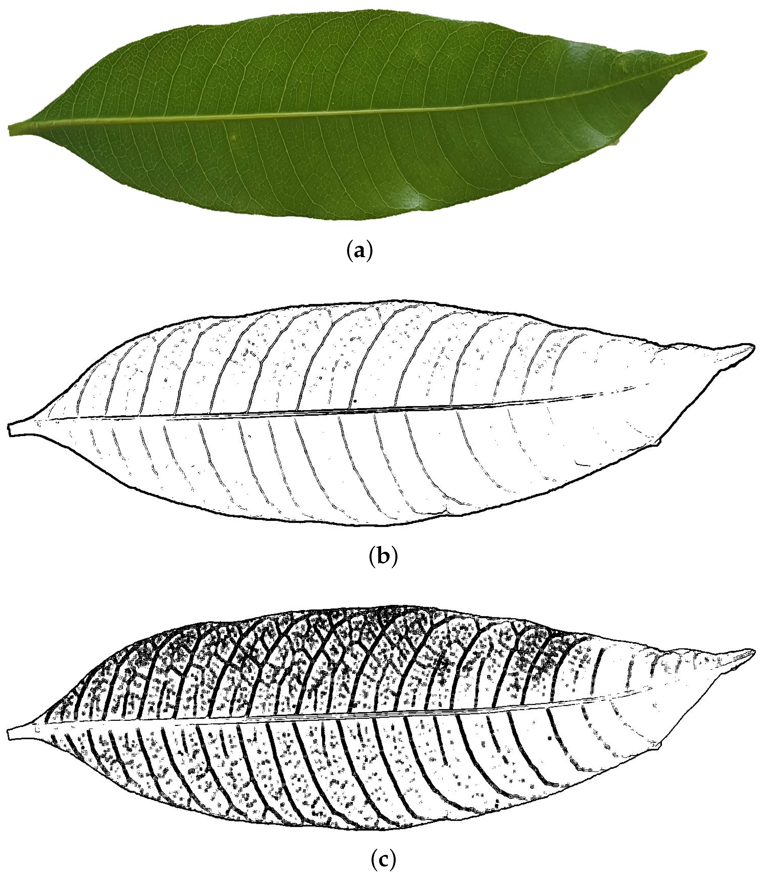
Further, a leaf image with more details is chosen next to evaluate the performance of the two segmentation methods. Figure 10a shows an original image of a leaf with complex texture and irregular edges, which puts high demands on the segmentation algorithm. Figure 10b,c shows the results of the segmentation of this leaf image using the gradient method and MF-AC-DFA method, respectively. As can be seen from Figure 10b, the gradient method has some limitations in processing the leaf image. Although it can roughly outline the blade, it does not perform well in the internal detail part of the blade. In contrast, the MF-AC-DFA method shows significant advantages in the segmentation of leaf images. As shown in Figure 10c, the method not only successfully extracts the overall contour of the leaf blade but also performs well in the internal details of the leaf. The texture and vein structure on the surface of the blade are better preserved, and the segmentation results are more fine and realistic. In summary, there is little difference between the two segmentation methods when targeting simple segmentation goals. However, when dealing with images with more details, especially through the segmentation experiments of leaf images, it can be concluded that the MF-AC-DFA method shows significant advantages. It outperforms the traditional gradient method in terms of detail retention and vein recognition. This indicates that the MF-AC-DFA method has strong accuracy compared to the gradient method and is suitable for many types of image segmentation tasks, especially in natural scenes with application potential.
Figure 10.
A comparison of two segmentation algorithms in a leaf. (a) A leaf image. (b) The result of (a) using the gradient method. (c) The result of (a) using MF-AC-DFA.
3.3. Applicability Experiments of MF-AC-DFA
The sagging effect of a wire is the arc formed by the natural sagging of the wire between two fixed points. Excessive sag may result in insufficient distance between the wire and the ground, buildings, or other obstacles, which may cause short circuits, electric shock accidents, and even injuries or property damage []. The variation in arc sag on electric wires is a complex phenomenon that is influenced by several factors. It has been shown that an increase in temperature leads to thermal expansion of the conductor, which increases the arc sag []. In addition, the plastic elongation of the material caused by the aging of the conductor also leads to a gradual increase in the arc sag []. The image segmentation technology can separate the wires from different backgrounds, which is conducive to calculating the arc droop of the wires, facilitating the calculation of the arc droop, and combining the temperature, aging degree, and other data for comprehensive analysis, so as to effectively assess the safety of the electric wire. Therefore, it is necessary to perform a segmentation of wire diagrams.
In this subsection, the focus is on evaluating the effectiveness of the proposed algorithm for wire image segmentation under different backgrounds. To fully validate its performance, experiments are conducted in two scenarios, simple background and complex background, respectively. The target images used for segmentation in the following experiments were taken from a paper by Zanella et al. []
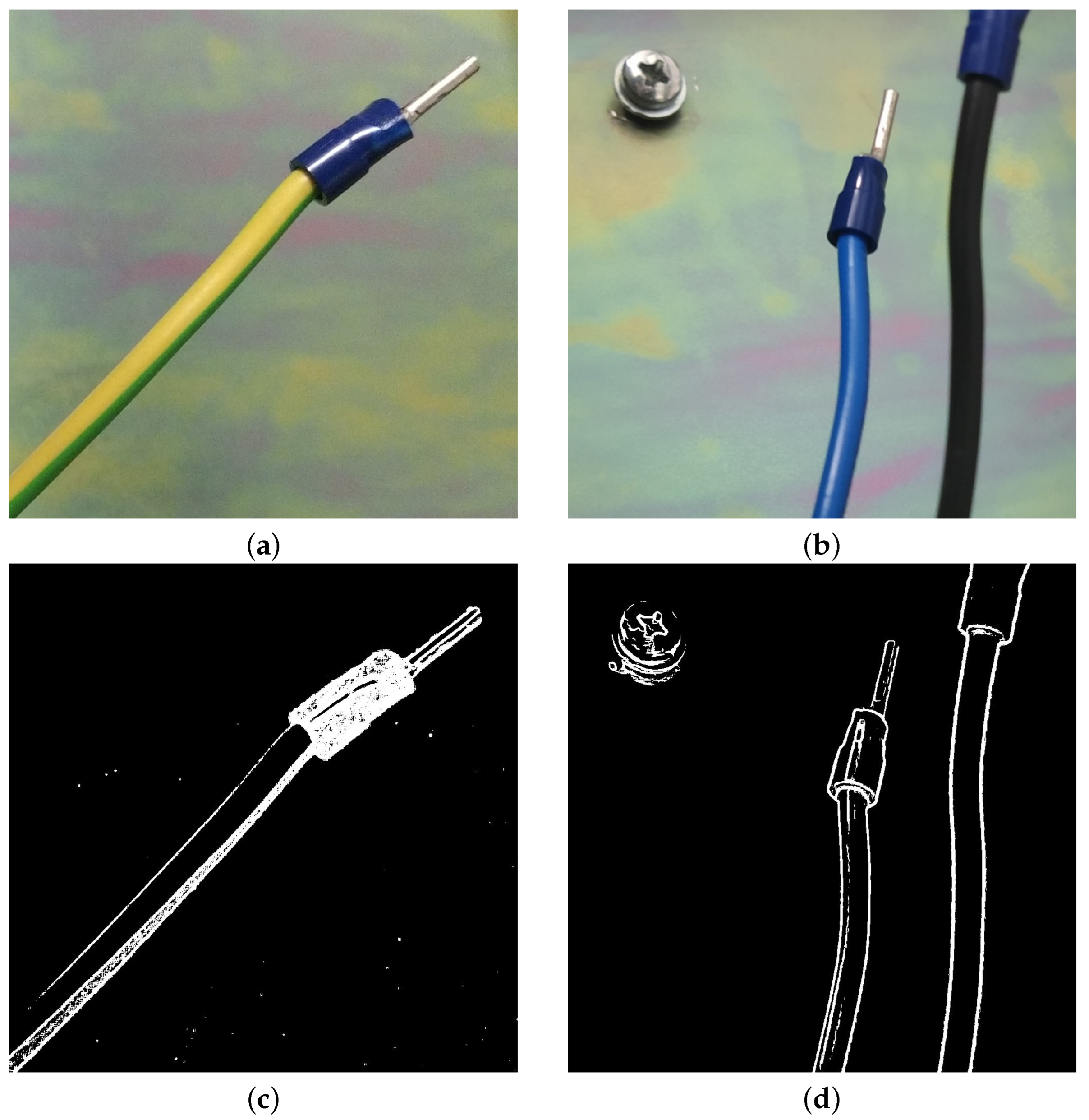
First, two images of wires with simple backgrounds are sought, as shown in Figure 11a,b. The final image segmentation results are shown in Figure 11c,d. As can be seen from the results in Figure 11c, this experiment successfully separates the three parts of this electric wire from the background, i.e., the three parts of silicone tubing, insulating tape, and pins are identified. The segmentation result illustrated in Figure 11d yields the three components of the wire as well as the screw in the background, and our method overall yields satisfactory segmentation results. These two segmentation results of the electric wire with simple backgrounds show that the proposed MF-AC-DFA algorithm is effective.
Figure 11.
Image segmentation of electric wire images on simple backgrounds. (a) Single-electric wire image. (b) Two-electric wire image. Contour line image of (a). (c) Segmented image of (a). (d) Segmented image of (b).
It is important to note that the background of the wire image is artificially controllable. Nevertheless, it is necessary to consider the segmentation of wires in very complex backgrounds. Figure 12 illustrates the overall segmentation results. First, we apply the MF-AC-DFA method for initial segmentation. Figure 12c,g show that although MF-AC-DFA can extract the wire contour completely, there is still noise in the background, which affects the purity of the segmentation results. To further optimize the segmentation effect, consider introducing morphological operations as a postprocessing step. By first performing MF-AC-DFA and then combining with morphological operations, very ideal segmentation results are finally obtained; see Figure 12d,h. To ensure the scientific validity of the experiments, the direct use of morphological manipulation is also tested. However, as shown in Figure 12b,f, the method fails to achieve the desired results, and its performance is not as good as using MF-AC-DFA alone. This suggests that it is difficult to efficiently separate wires from the background by relying only on morphological operations in complex backgrounds, whereas MF-AC-DFA can more accurately capture the wire feature information.
Figure 12.
Image segmentation of electric wire images on complex backgrounds. (a) Yellow line in complex background image. (b) Direct morphological manipulation result of (a). (c) MF-AC-DFA result of (a). (d) MF-AC-DFA followed by morphological manipulation result of (a). (e) White line in complex background image. (f) Direct morphological manipulation result of (e). (g) MF-AC-DFA result of (a). (h) MF-AC-DFA followed by morphological manipulation result of (e).
In conclusion, the image segmentation algorithm used in this experiment shows good segmentation results under simple background conditions for both single- and two-wire images by effectively extracting the edge information of the wires. When facing very complex backgrounds, although the complete wire contour can be segmented, the background noise still exists, and the performance of the algorithm will be affected to some extent. However, after the proposed algorithm is combined with morphological operations, excellent results are obtained.
By conducting image segmentation experiments of transmission towers with different shooting perspectives and under different weather, the overall structure of the tower can be separated from these backgrounds, which is the basis for recognizing the tower and its surroundings and also an important prerequisite for condition monitoring. The aging and corrosion of transmission towers often first manifests itself in changes in appearance, such as the deformation of the tower body and surface corrosion. These changes will be directly reflected in the profile. By segmenting the images of transmission towers, it is possible not only to accurately identify transmission towers and their surroundings but also to monitor the status of transmission towers. As a result, we predict the possible aging and corrosion problems of the transmission tower and develop a maintenance plan accordingly. This helps to extend the service life of transmission towers and reduce maintenance costs.
The following section focuses on testing the segmentation effect of the proposed algorithm on transmission tower images under different shooting viewpoints and different meteorological conditions. Firstly, two typical viewpoints, elevation and top view, are selected for analysis. Then, weather factors such as rain, snow, haze, etc., also degrade the image quality [,,], thus affecting the accuracy and stability of the segmentation results. Thus, to comprehensively evaluate the performance of the algorithm, experiments were conducted under various conditions such as less cloudy and cloudy, light and no light, fog and no fog, etc., to verify the robustness and effectiveness of the proposed method in complex real-world scenes. The transmission tower images used for segmentation are from the Transmission Towers and Power Lines Aerial-image Dataset (TTPLA), an open-source aerial-image dataset focusing on the detection and segmentation of transmission towers and power lines. The project is powered by the InsCode AI Big Model developed by CSDN, Inc. (Beijing, China).
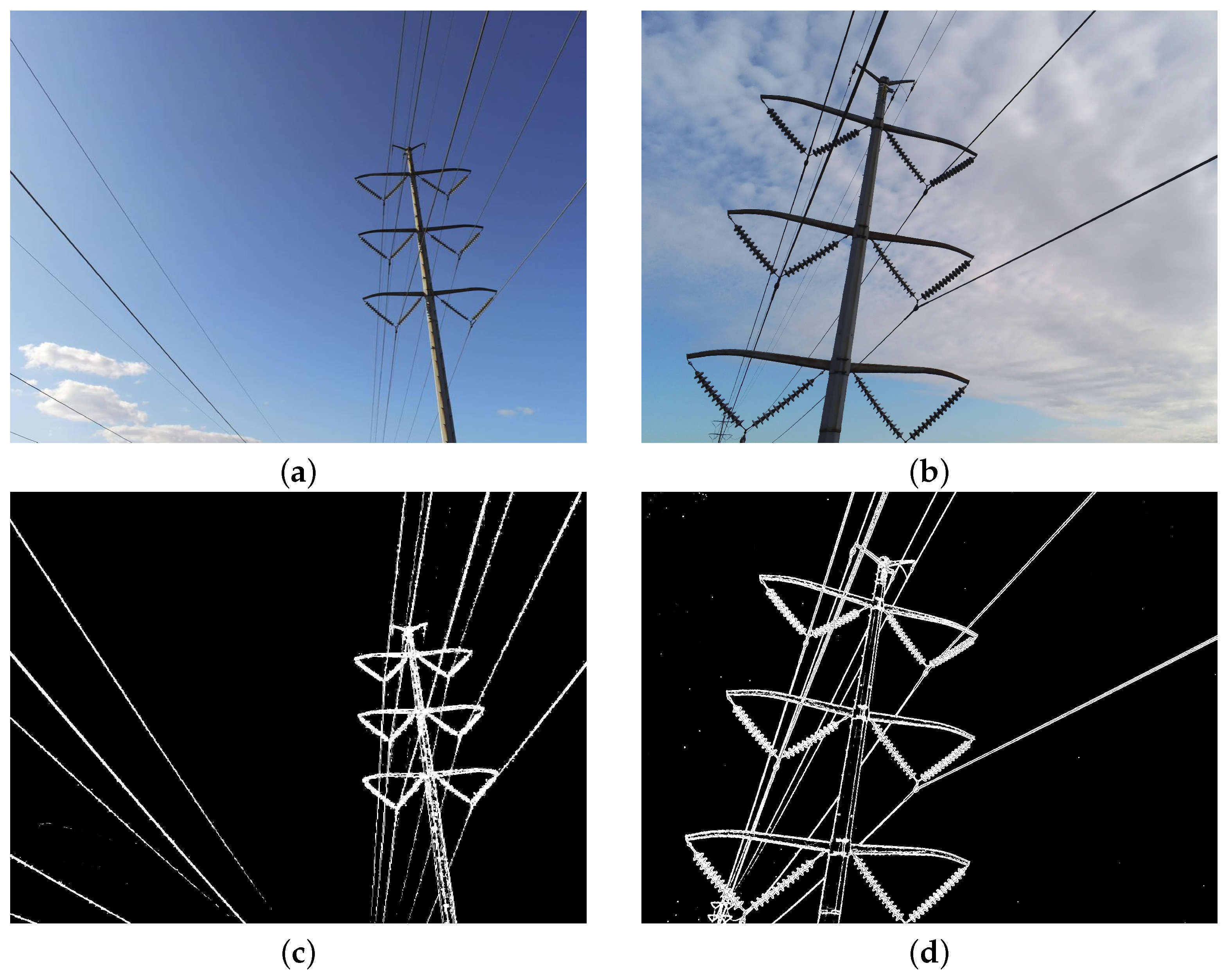
As shown in Figure 13, image segmentation experiments have been performed on transmission tower images from both the elevated and overhead viewpoints. Figure 13a shows an elevation viewpoint image and Figure 13b shows a top viewpoint image. Figure 13c,d show the segmentation results for the upward view and downward view images with different algorithm parameters, respectively. Despite the noise in the segmented image in the overhead view and the imperfect segmentation of the lower half of the transmission tower, the algorithm successfully segments the upper half and presents the main structure. This shows that the algorithm is adaptive under certain conditions and can maintain good performance in different shooting angles to accurately recognize the main structure.
Figure 13.
Transmission tower image segmentation in elevation and overhead shots. (a) Elevated image. (b) Overhead image. (c) Segmented image of (a). (d) Segmented image of (b).
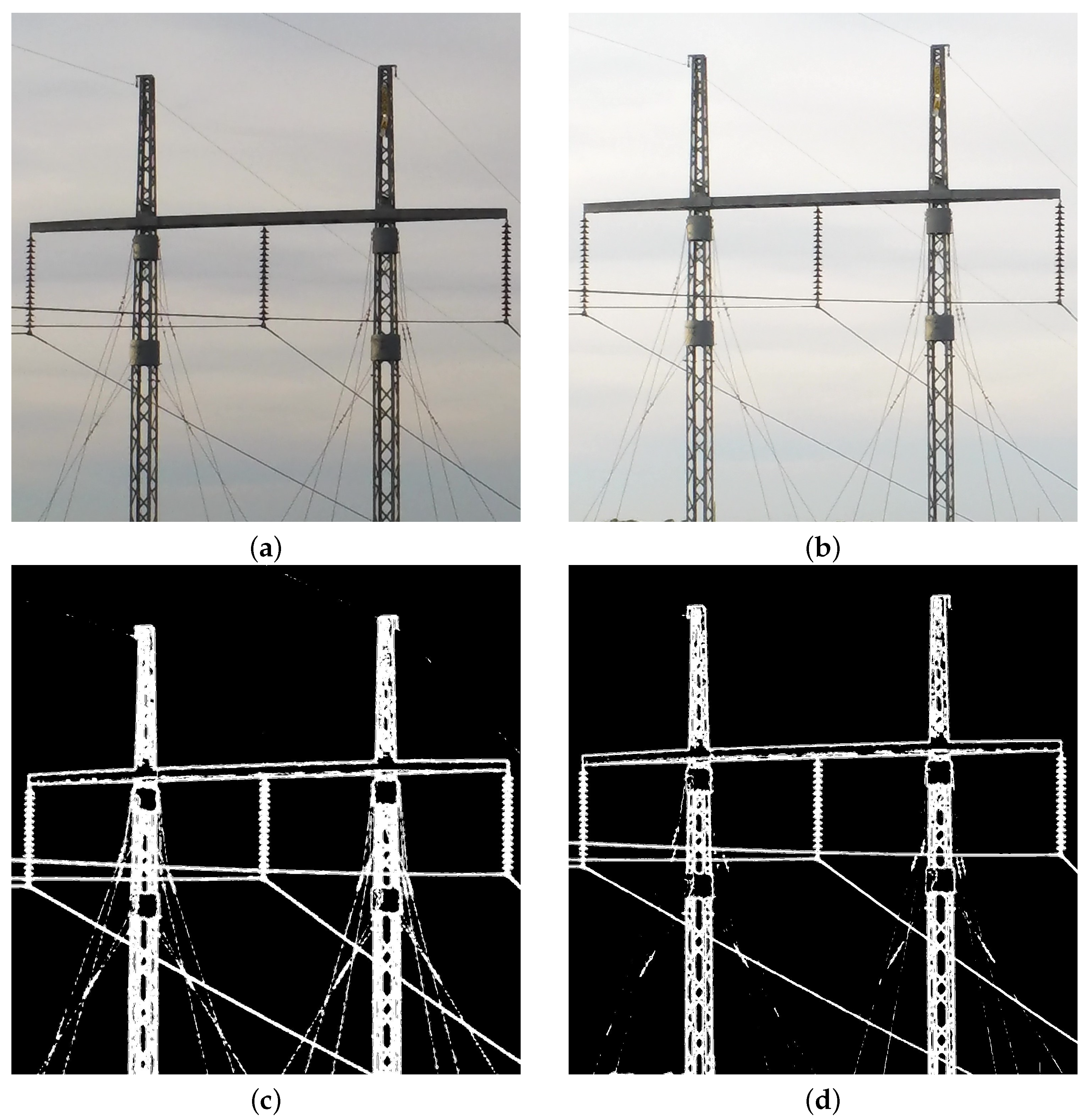
Next, the performance of the proposed algorithm is evaluated under less and more cloudy backgrounds. As shown in Figure 14, image segmentation experiments are conducted on transmission tower images under less cloudy and more cloudy weather, respectively. Specifically, Figure 14a shows a less cloudy transmission tower image and Figure 14b shows a more cloudy transmission tower image. Figure 14c,d show the transmission tower segmentation results for less cloudy and more cloudy with different algorithm parameters. From the segmentation results, it can be seen that the algorithm can effectively recognize and separate the main structural parts of the transmission towers under both less cloudy and more cloudy backgrounds. Although the cloudy background increases the complexity of the image, the algorithm is still able to segment the main structure of the transmission tower, indicating that the proposed algorithm has strong robustness and adaptability.
Figure 14.
Transmission tower image segmentation with less cloudy and cloudy backgrounds. (a) Few-cloud background image. (b) Cloudy background image. (c) Segmented image of (a). (d) Segmented image of (b).
Further, the segmentation results of the algorithm under different lighting conditions are explored. As shown in Figure 15, image segmentation experiments were conducted on transmission tower images under unlit and lit conditions. Figure 15a shows an image of a transmission tower with an unlit background and Figure 15b shows an image with a lit background. Applying the segmentation algorithm with different parameters, Figure 15c,d show the final segmentation results, respectively. The results show that the algorithm is effective in identifying and separating the main structural parts of the transmission tower under both the unlit and lit conditions. However, compared to Figure 15d, the details of the wires in the lower part of the transmission tower in Figure 15c are not clear enough, which may be due to the highlights caused by the illumination affecting the segmentation results. Although the lighting conditions increase the complexity of the image, the algorithm still clearly segments the main structure of the transmission tower, indicating that the algorithm is robust and adaptable.
Figure 15.
Transmission tower image segmentation with unlit and lit backgrounds. (a) Unlit background image. (b) Lit background image. (c) Segmented image of (a). (d) Segmented image of (b).
Finally, the performance of our proposed algorithm is evaluated in fog-free and foggy backgrounds. As shown in Figure 16, we conducted image segmentation experiments on transmission tower images under fog-free and foggy weather, respectively. Specifically, Figure 16a shows an image of a transmission tower in a fog-free background and Figure 16b shows an image in a foggy background. By applying our segmentation algorithm, Figure 16c,d show the final segmentation results. The computational results show that the method can effectively recognize and separate the main structure of the transmission tower in both fog-free and foggy backgrounds. However, the foggy condition increases the complexity of the image, which results in the loss of some detailed information, for example, the thin line part in Figure 16d is not as clear as that in Figure 16c, and the part of the wire on the right side of the original image is lost in Figure 16d. However, our algorithm is still able to accurately segment the main structure of the transmission tower, which shows its robustness.
Figure 16.
Transmission tower image segmentation in fog-free and foggy backgrounds. (a) Fog-free background image. (b) Foggy background image. (c) Segmented image of (a). (d) Segmented image of (b).
Through the above experiments, the proposed algorithm is validated under a variety of shooting viewpoints and environmental conditions. The results show that the algorithm can effectively segment the main body of the transmission tower in both elevated and overhead views and can still clearly present the upper half of the structure even when there is noise and poor segmentation of the lower half of the tower in the overhead view. The algorithm maintains good segmentation performance in both cloudy and cloudy backgrounds; even in light conditions with some detail flaws, the overall body of the tower can still be accurately extracted. In addition, the algorithm also shows strong robustness in foggy and fog-free environments and can cope with the challenges of low visibility. In summary, this algorithm shows good adaptability and practicability in complex scenes and provides a reference for the practical application of transmission tower image segmentation.
4. Conclusions
This study introduces a novel image segmentation method, termed MF-AC-DFA, which integrates the MF-DFA combined with the AC equation. By substituting the traditional least squares method with the AC equation for fitting purposes, we have achieved significant improvements in both the accuracy and robustness of image segmentation. The feasibility of MF-AC-DFA is rigorously tested under diverse conditions, encompassing various target shapes, image backgrounds, and resolutions. These comprehensive experiments underscore the versatility and reliability of our proposed method across a wide range of scenarios. Furthermore, comparative analyses with the gradient segmentation method highlighted the superior performance of MF-AC-DFA and demonstrated its enhanced capabilities in handling complex image segmentation tasks. To further validate the practical application potential of MF-AC-DFA, we applied it to real-life electric wire images and transmission tower diagrams. The successful segmentation of these complex scenes underscores the method’s robustness and applicability in real-world contexts, particularly in the domain of power facility monitoring. Given these promising results, we anticipate that MF-AC-DFA will play a pivotal role in the real-time state monitoring and analysis of power facilities. By enhancing the accuracy and reliability of image segmentation, this method holds the potential to significantly improve the safety and reliability of the power grid. Although the method has some limitations in calculating more complex situations, its good performance and wide application prospects provide valuable references for its practical application. Future work may focus on further optimizing the computational efficiency of MF-AC-DFA and exploring its applications in other critical infrastructure domains.
Author Contributions
Conceptualization, M.W., J.W. and J.K.; Data curation, Y.W.; Formal analysis, M.W. and J.W.; Funding acquisition, J.W.; Investigation, R.X. and R.P.; Methodology, J.W.; Project administration, M.W. and J.W.; Resources, M.W., J.W. and J.K.; Software, M.W.; Supervision, J.K.; Validation, Y.W.; Visualization, R.X. and R.P.; Writing —original draft, Y.W.; Writing—review & editing, J.W. All authors have read and agreed to the published version of the manuscript.
Funding
The author Minzhen Wang expresses thanks for the Management Technology Project of State Grid Liaoning Electric Power Co., LTD., project No. 2023YF-11. The author Jian Wang expresses thanks for The Natural Science Foundation of Jiangsu Province (Grants No BK20240689). The corresponding author (J.S. Kim) was supported by the National Research Foundation(NRF), Korea, under project BK21 FOUR.
Data Availability Statement
The raw data supporting the conclusions of this article will be made available by the authors on request.
Conflicts of Interest
The authors declare no conflicts of interest.
Abbreviations
The following abbreviations are used in this manuscript:
| MF-DFA | Multifractal detrended fluctuation |
| MF-AC-DFA | Multifractal detrended fluctuation combined with Allen–Cahn equation |
| MF-DCCA | Multifractal Detrended Cross-Correlation Analysis |
| UAV | Unmanned Aerial Vehicle |
| IOT | Internet of Things |
| mIOU | Mean Intersection Over Union |
| mDice | Mean Dice Coefficient |
| MF-LSSVM-DFA | Multifractal least squares support vector machine detrended fluctuation analysis |
References
- Roy, S.; Kundu, C.K. State of the art review of wind induced vibration and its control on transmission towers. Structures 2021, 29, 254–264. [Google Scholar] [CrossRef]
- Tian, L.; Pan, H.; Ma, R.; Zhang, L.; Liu, Z. Full-scale test and numerical failure analysis of a latticed steel tubular transmission tower. Eng. Struct. 2020, 208, 109919. [Google Scholar] [CrossRef]
- Wang, M.; Gao, H.; Wang, Z.; Yue, K.; Zhong, C.; Zhang, G.; Wang, J. Correlation between Temperature and the Posture of Transmission Line Towers. Symmetry 2024, 16, 1270. [Google Scholar] [CrossRef]
- Damodaran, S.; Shanmugam, L.; Parkavi, K.; Venkatachalam, N.; Swaroopan, N.J. Segmentation of Transmission Tower Components Based on Machine Learning. In Machine Learning Hybridization and Optimization for Intelligent Applications, 1st ed.; CRC Press: Boca Raton, FL, USA, 2024; pp. 182–198. [Google Scholar]
- Ma, W.; Xiao, J.; Zhu, G.; Wang, J.; Zhang, D.; Fang, X.; Miao, Q. Transmission tower and Power line detection based on improved Solov2. IEEE Trans. Instrum. Meas. 2024, 73, 5015711. [Google Scholar] [CrossRef]
- He, M.; Qin, L.; Deng, X.; Zhou, S.; Liu, H.; Liu, K. Transmission line segmentation solutions for uav aerial photography based on improved unet. Drones 2023, 7, 274. [Google Scholar] [CrossRef]
- Vahab, S.; Sankaran, A. Multifractal Applications in Hydro-Climatology: A Comprehensive Review of Modern Methods. Fractal Fract. 2025, 9, 27. [Google Scholar] [CrossRef]
- Wang, F.; Chang, J.; Zuo, W.; Zhou, W. Research on Efficiency and Multifractality of Gold Market under Major Events. Fractal Fract. 2024, 8, 488. [Google Scholar] [CrossRef]
- Han, C.; Xu, Y. Nonlinear Analysis of the US Stock Market: From the Perspective of Multifractal Properties and Cross-Correlations with Comparisons. Fractal Fract. 2025, 9, 73. [Google Scholar] [CrossRef]
- Wang, M.; Zhong, C.; Yue, K.; Zheng, Y.; Jiang, W.; Wang, J. Modified MF-DFA model based on LSSVM fitting. Fractal Fract. 2024, 8, 320. [Google Scholar] [CrossRef]
- Yue, K.; Wang, Z.; Yuan, P.; Gao, F.; Jia, Y.; Xu, Z.; Li, S. A Novel Infrared Image Segmentation Algorithm for Substation Equipment. In Proceedings of the 2024 Second International Conference on Cyber-Energy Systems and Intelligent Energy (ICCSIE), Shenyang, China, 17–19 May 2024. [Google Scholar]
- Yu, Y.E.; Wang, F.; Liu, L.L. Magnetic resonance image segmentation using multifractal techniques. Appl. Surf. Sci. 2015, 356, 266–272. [Google Scholar] [CrossRef]
- Yu, M.; Xing, L.; Wang, L.; Zhang, F.; Xing, X.; Li, C. An improved multifractal detrended fluctuation analysis method for estimating the dynamic complexity of electrical conductivity of karst springs. J. Hydroinformatics 2023, 25, 174–190. [Google Scholar] [CrossRef]
- Rak, R.; Zięba, P. Multifractal flexibly detrended fluctuation analysis. arXiv 2015, arXiv:1510.05115. [Google Scholar] [CrossRef]
- Allen, S.M.; Cahn, J.W. A microscopic theory for antiphase boundary motion and its application to antiphase domain coarsening. Acta Metall. 1979, 27, 1085–1095. [Google Scholar] [CrossRef]
- Uzunca, M.; Karasözen, B. Linearly implicit methods for Allen-Cahn equation. Appl. Math. Comput. 2023, 450, 127984. [Google Scholar] [CrossRef]
- Yang, J.; Kang, S.; Kwak, S.; Kim, J. The Allen–Cahn equation with a space-dependent mobility and a source term for general motion by mean curvature. J. Comput. Sci. 2024, 77, 102252. [Google Scholar] [CrossRef]
- Olshanskii, M.; Xu, X.; Yushutin, V. A finite element method for Allen–Cahn equation on deforming surface. Comput. Math. Appl. 2021, 90, 148–158. [Google Scholar] [CrossRef]
- Song, X.; Xia, B.; Li, Y. An efficient data assimilation based unconditionally stable scheme for Cahn–Hilliard equation. Comput. Appl. Math. 2024, 43, 121. [Google Scholar] [CrossRef]
- Favre, G.; Schimperna, G. On a Navier-Stokes-Allen-Cahn model with inertial effects. J. Math. Anal. Appl. 2019, 475, 811–838. [Google Scholar] [CrossRef]
- Poochinapan, K.; Wongsaijai, B. Numerical analysis for solving Allen-Cahn equation in 1D and 2D based on higher-order compact structure-preserving difference scheme. Appl. Math. Comput. 2022, 434, 127374. [Google Scholar] [CrossRef]
- Lv, Z.; Song, X.; Feng, J.; Xia, Q.; Xia, B.; Li, Y. Reduced-order prediction model for the Cahn–Hilliard equation based on deep learning. Eng. Anal. Bound. Elem. 2025, 172, 106118. [Google Scholar] [CrossRef]
- Kim, J. Modified wave-front propagation and dynamics doming from higher-order double-well potentials in the Allen–Cahn equations. Mathematics 2024, 12, 3796. [Google Scholar] [CrossRef]
- Jin, Y.; Kwak, S.; Ham, S.; Kim, J. A fast and efficient numerical algorithm for image segmentation and denoising. AIMS Math. 2024, 9, 5015–5027. [Google Scholar] [CrossRef]
- Chen, Y.; Ding, X. A survey of sag monitoring methods for power grid transmission lines. IET Gener. Transm. Distrib. 2023, 17, 1419–1441. [Google Scholar] [CrossRef]
- Noor, B.; Abbasi, M.Z.; Qureshi, S.S.; Ahmed, S. Temperature and wind impacts on sag and tension of AAAC overhead transmission line. Int. J. Adv. Appl. Sci. 2018, 5, 14–18. [Google Scholar] [CrossRef]
- Muhr, H.M.; Pack, S.; Jaufer, S. Sag calculation of aged overhead lines. In Proceedings of the 14th International Symposium on High Voltage Engineering, Beijing, China, 25–29 August 2005; Tsinghua University Press: Beijing, China; p. 206. [Google Scholar]
- Zanella, R.; Caporali, A.; Tadaka, K.; De Gregorio, D.; Palli, G. Auto-generated wires dataset for semantic segmentation with domain-independence. In Proceedings of the 2021 International Conference on Computer, Control and Robotics (ICCCR), Shanghai, China, 8–10 January 2021. [Google Scholar]
- Popoff, S.M.; Lerosey, G.; Carminati, R.; Fink, M.; Boccara, A.C.; Gigan, S. Measuring the Transmission Matrix in Optics: An Approach to the Study and Control of Light Propagation in Disordered Media. Phys. Rev. Lett. 2010, 104, 100601. [Google Scholar] [CrossRef]
- Galaktionov, I.; Nikitin, A.; Sheldakova, J.; Toporovsky, V.; Kudryashov, A. Focusing of a laser beam passed through a moderately scattering medium using phase-only spatial light modulator. Photonics 2022, 9, 296. [Google Scholar] [CrossRef]
- Vellekoop, I.M. Feedback-based wavefront shaping. Opt. Express 2015, 23, 12189–12206. [Google Scholar] [CrossRef]
Disclaimer/Publisher’s Note: The statements, opinions and data contained in all publications are solely those of the individual author(s) and contributor(s) and not of MDPI and/or the editor(s). MDPI and/or the editor(s) disclaim responsibility for any injury to people or property resulting from any ideas, methods, instructions or products referred to in the content. |
© 2025 by the authors. Licensee MDPI, Basel, Switzerland. This article is an open access article distributed under the terms and conditions of the Creative Commons Attribution (CC BY) license (https://creativecommons.org/licenses/by/4.0/).