


Multi-Focus Image Fusion Based on Fractal Dimension and Parameter Adaptive Unit-Linking Dual-Channel PCNN in Curvelet Transform Domain


Abstract
1. Introduction
2. Related Work
2.1. Curvelet Transform
2.2. PAUDPCNN
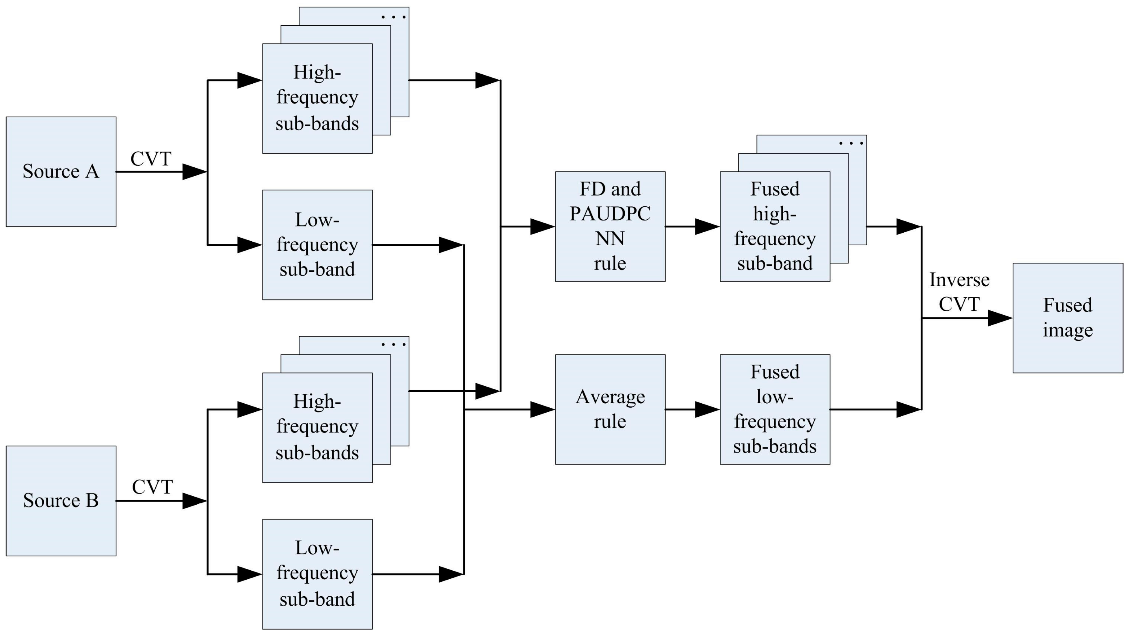
3. The Proposed Method
3.1. Image Decomposition
3.2. Fusion of High-Frequency Sub-Bands
3.3. Fusion of Low-Frequency Sub-Bands
3.4. Inverse CVT
| Algorithm 1: The proposed fusion method |
| Input: the source images: A and B Parameters: the number of CVT decomposition levels: L, the number of PAUDPCNN iterations: N Main step: Step 1: CVT decomposition For each source image Perform CVT on to generate ; End Step 2: High-frequency sub-bands’ fusion For each level For each direction For each source image Initialize the PAUDPCNN model: ; Estimate the PAUDPCNN parameters , , and via Equations (10)–(12); Compute the value of using Equations (9), (16)–(17); For each iterations Compute the PAUDPCNN model using Equations (3)–(8); End Get the decision map based on Equation (18); Perform the majority filtering on decision map to guarantee the consistency using Equation (19); Compute the fused high-frequency sub-bands according to Equation (20); End End End Step 3: Low-frequency sub-bands’ fusion For each source image Merge and using Equation (21) to generate End Step 4: Inverse CVT Perform inverse CVT on to obtain ; Output: the fused image . |
4. Experimental Results
4.1. Experimental Setup
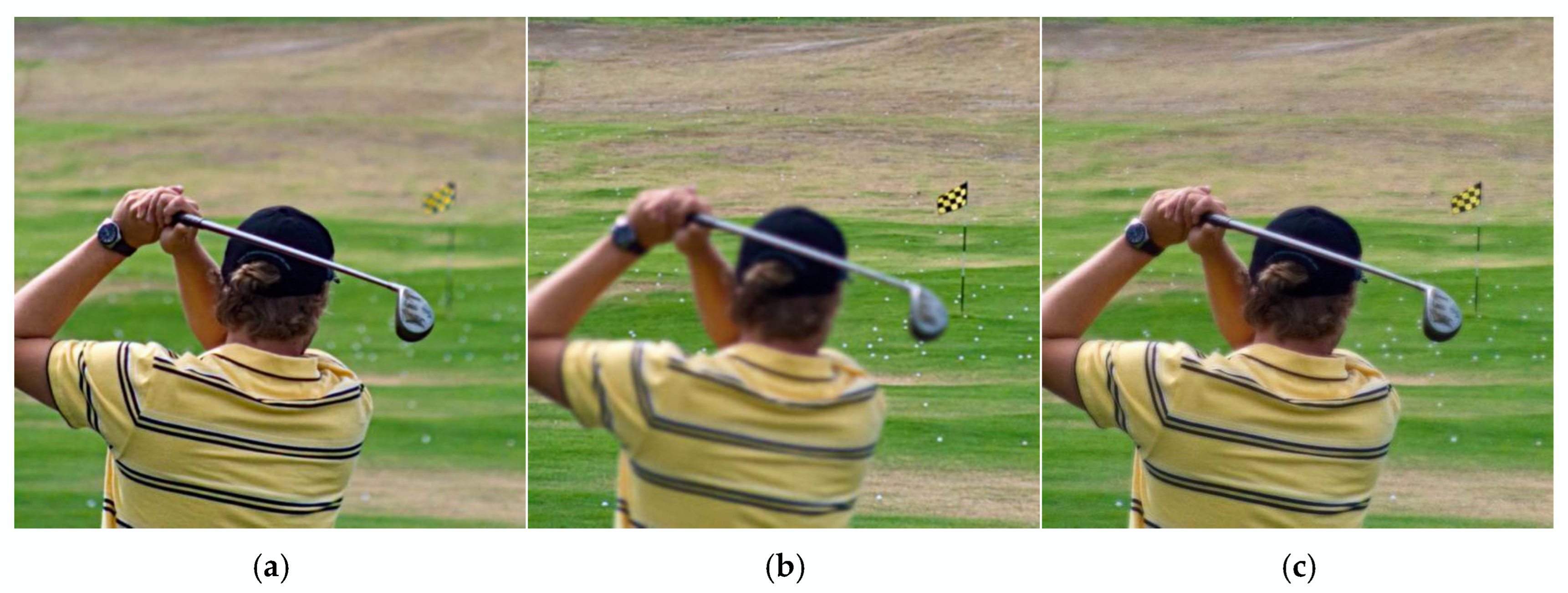
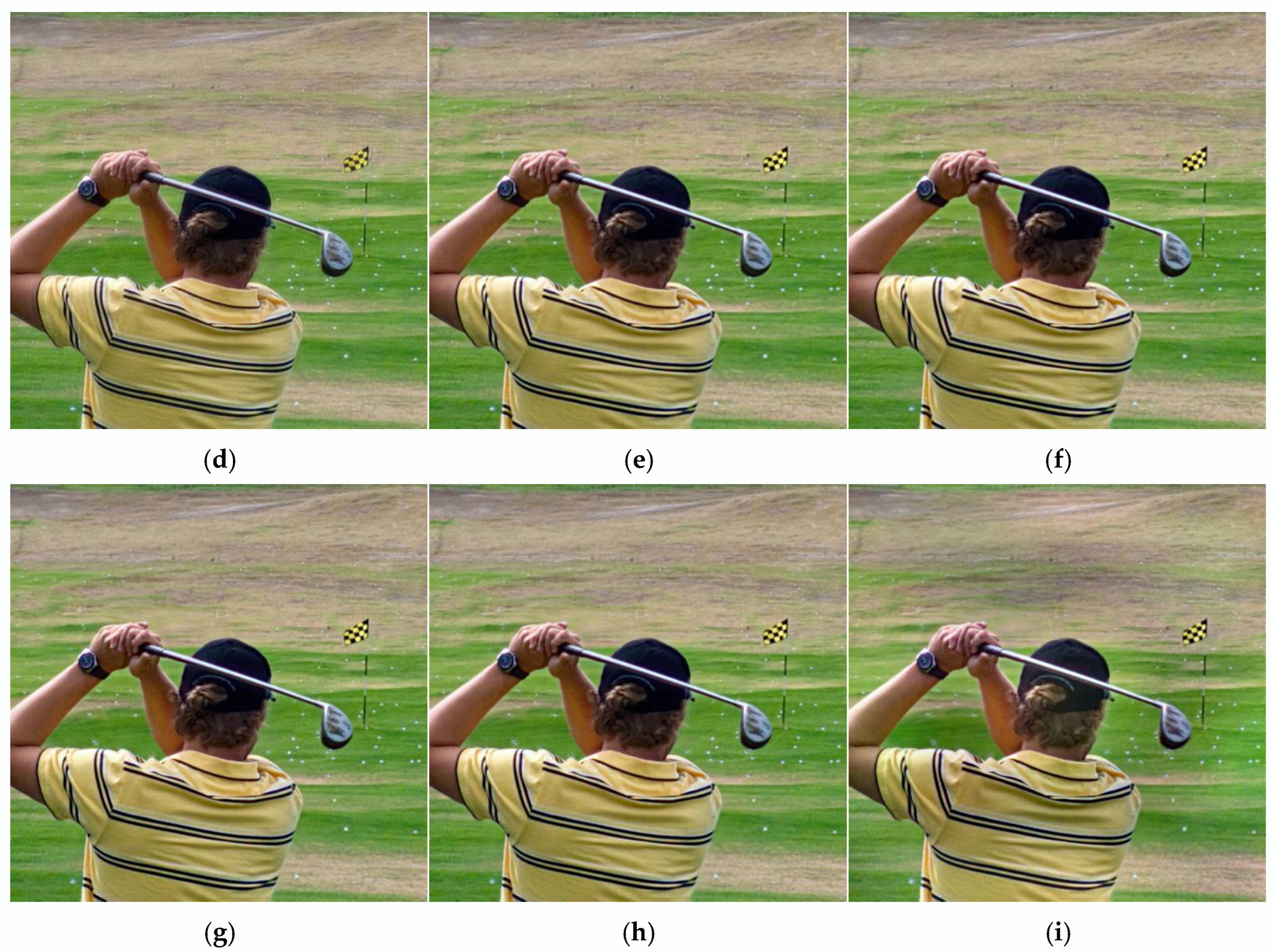
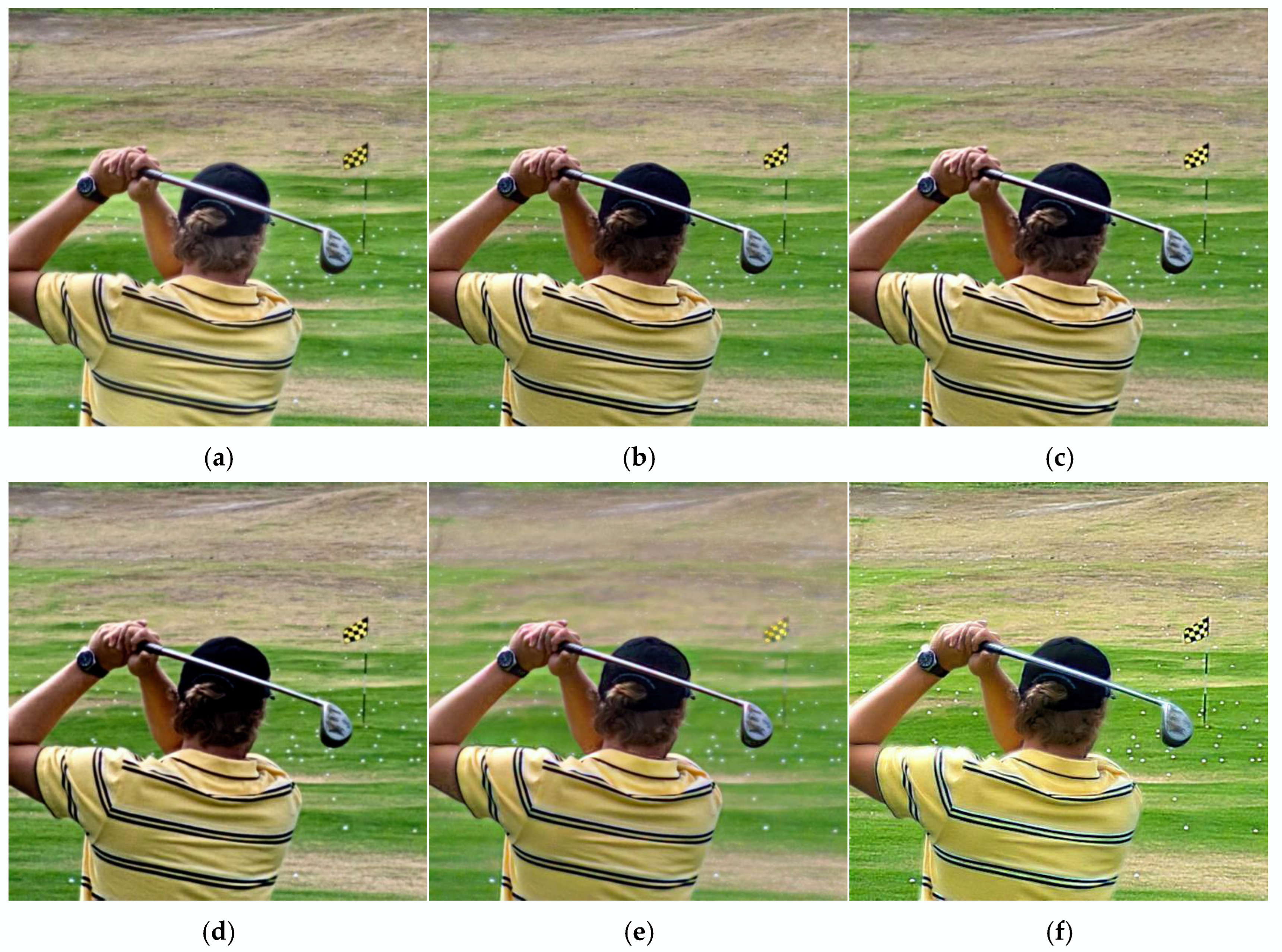
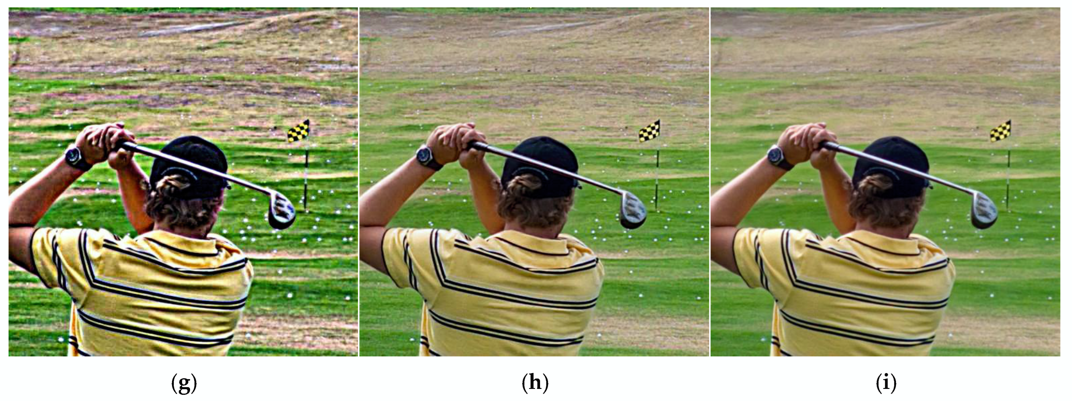
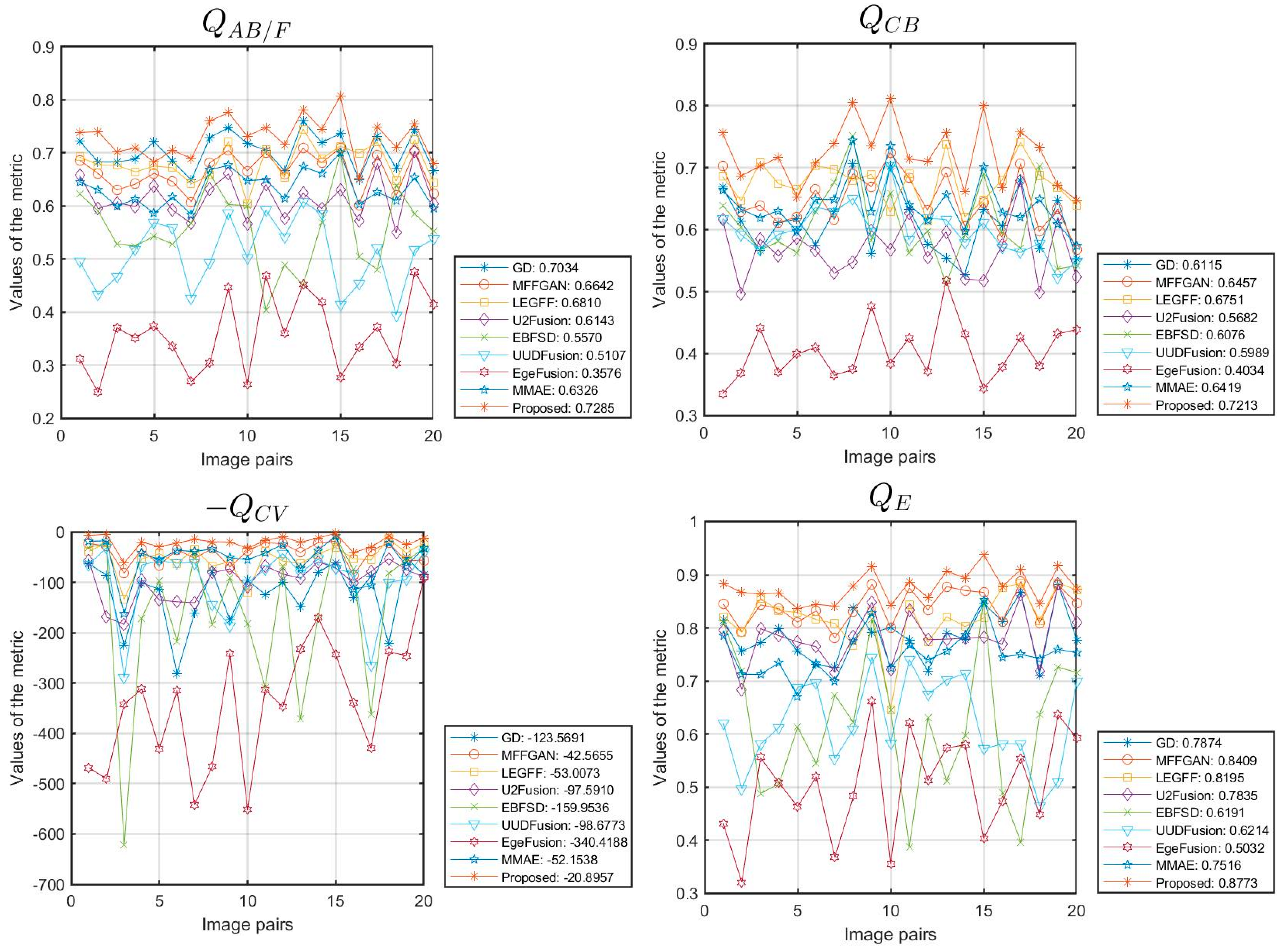
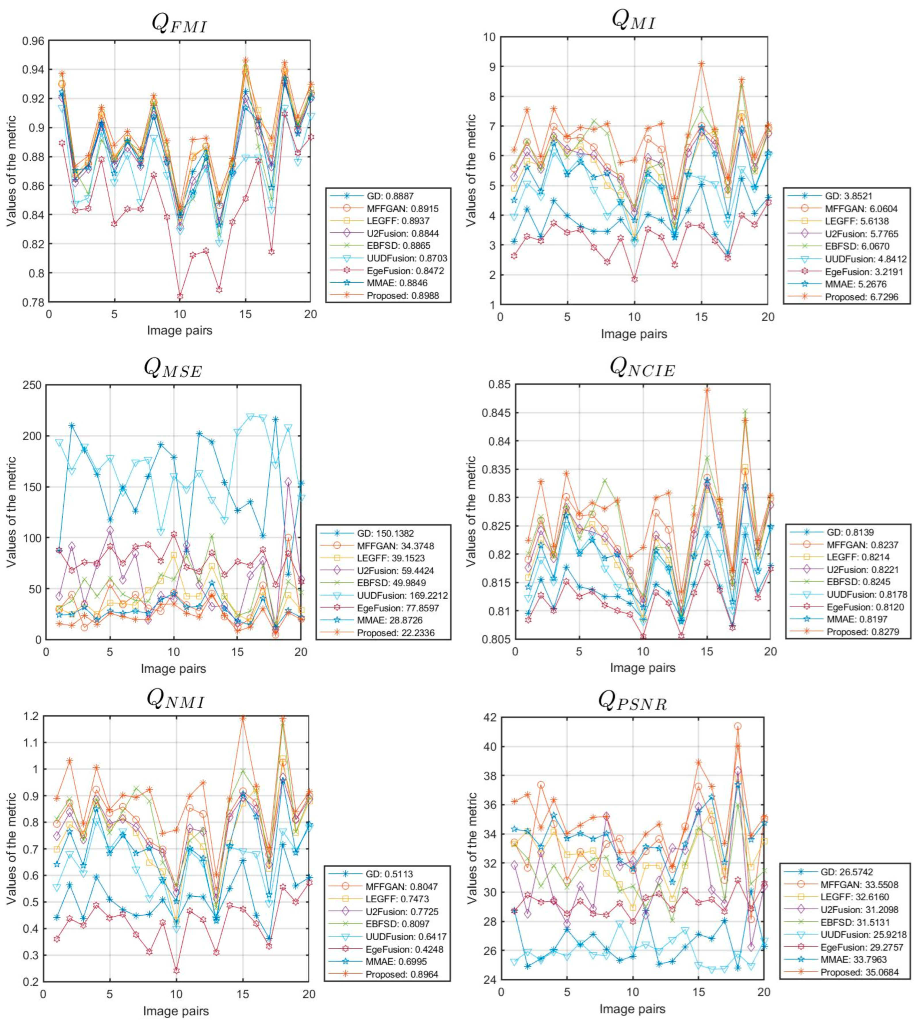
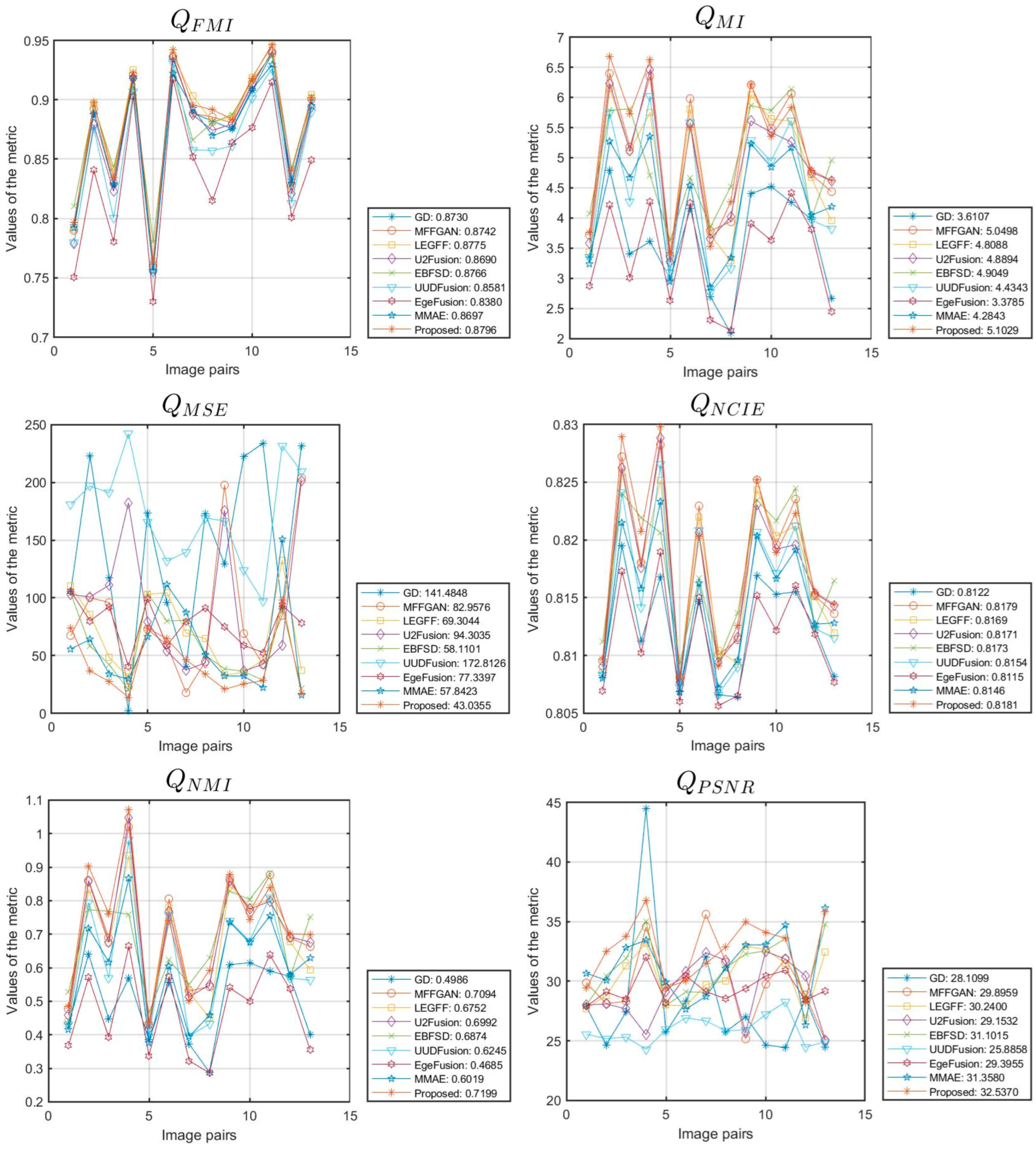
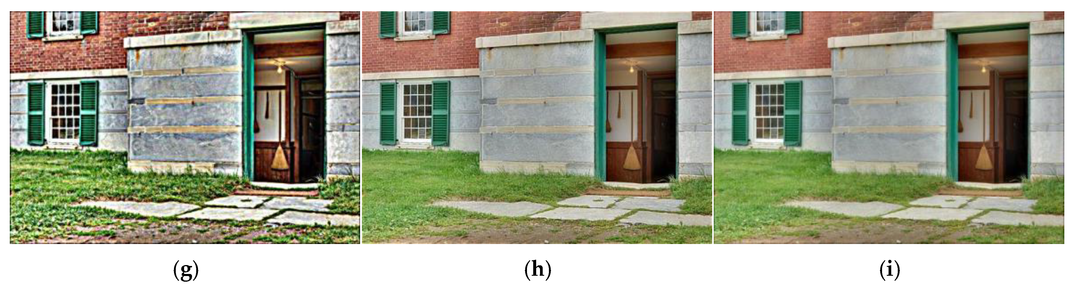
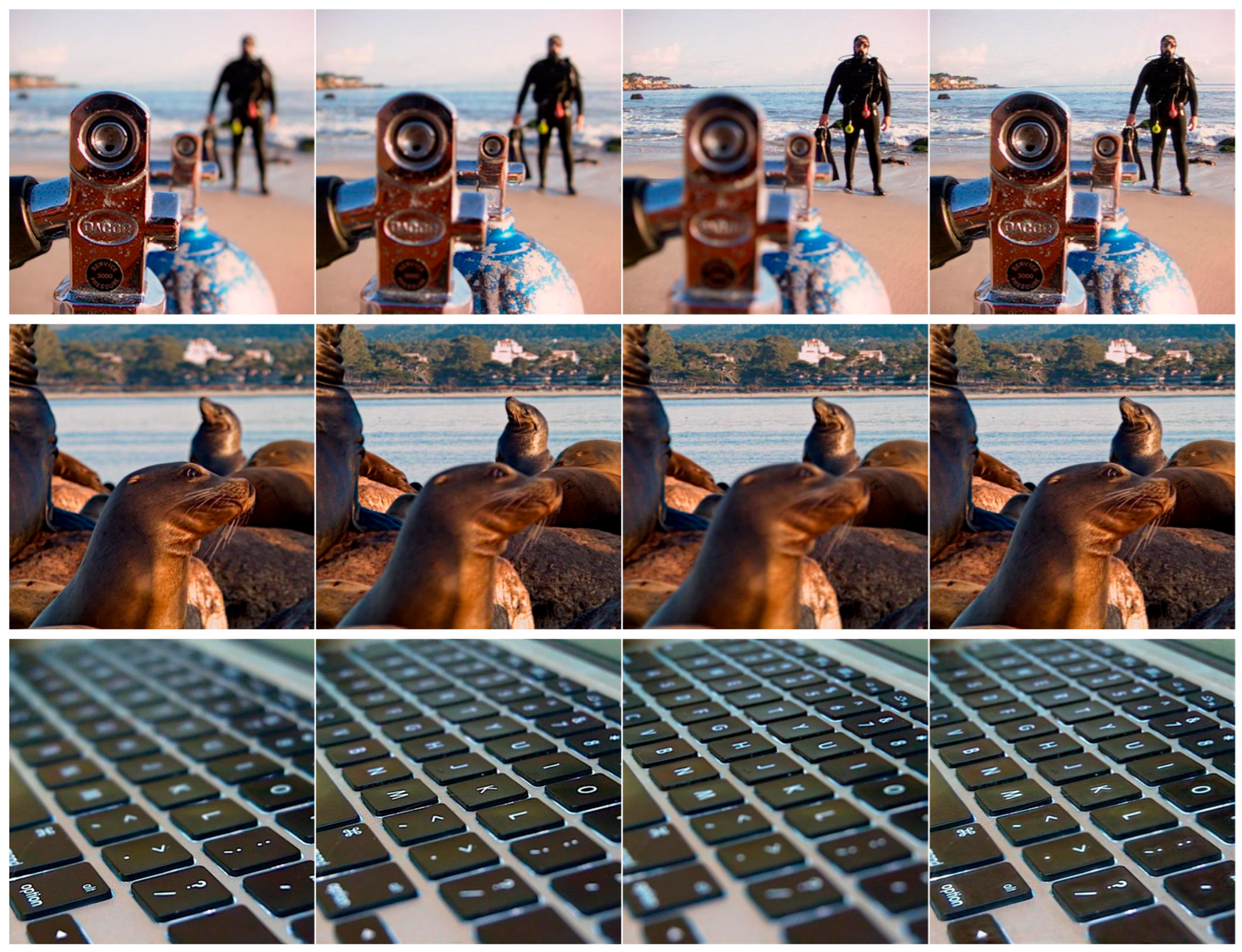
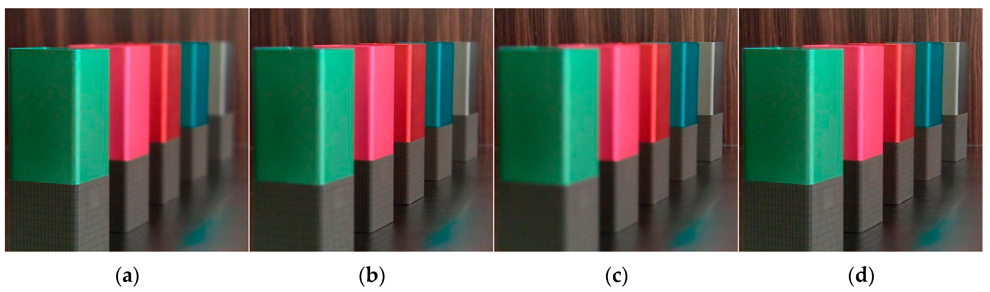
4.2. Fusion Results and Discussion
4.3. Application Extension
5. Conclusions
Author Contributions
Funding
Data Availability Statement
Conflicts of Interest
References
- Zhai, H.; Ouyang, Y.; Luo, N. MSI-DTrans: A multi-focus image fusion using multilayer semantic interaction and dynamic transformer. Displays 2024, 85, 102837. [Google Scholar] [CrossRef]
- Li, B.; Zhang, L.; Liu, J.; Peng, H. Multi-focus image fusion with parameter adaptive dual channel dynamic threshold neural P systems. Neural Netw. 2024, 179, 106603. [Google Scholar] [CrossRef] [PubMed]
- Wang, W.; Deng, L.; Vivone, G. A general image fusion framework using multi-task semi-supervised learning. Inf. Fusion 2024, 108, 102414. [Google Scholar] [CrossRef]
- Yan, H.; Zhang, J.; Zhang, X. Injected infrared and visible image fusion via L1 decomposition model and guided filtering. IEEE Trans. Comput. Imaging 2022, 8, 162–173. [Google Scholar] [CrossRef]
- Zhang, X.; He, H.; Zhang, J. Multi-focus image fusion based on fractional order differentiation and closed image matting. ISA Trans. 2022, 129, 703–714. [Google Scholar] [CrossRef] [PubMed]
- Zhang, X.; Yan, H. Medical image fusion and noise suppression with fractional-order total variation and multi-scale decomposition. IET Image Process. 2021, 15, 1688–1701. [Google Scholar] [CrossRef]
- Yan, H.; Zhang, X. Adaptive fractional multi-scale edge-preserving decomposition and saliency detection fusion algorithm. ISA Trans. 2020, 107, 160–172. [Google Scholar] [CrossRef]
- Zhang, X.; Yan, H.; He, H. Multi-focus image fusion based on fractional-order derivative and intuitionistic fuzzy sets. Front. Inf. Technol. Electron. Eng. 2020, 21, 834–843. [Google Scholar] [CrossRef]
- Li, H.; Wang, D.; Huang, Y.; Zhang, Y. Generation and recombination for multifocus image fusion with free number of inputs. IEEE Trans. Circuits Syst. Video Technol. 2024, 34, 6009–6023. [Google Scholar] [CrossRef]
- Li, H.; Shen, T.; Zhang, Z.; Zhu, X.; Song, X. EDMF: A new benchmark for multi-focus images with the challenge of exposure difference. Sensors 2024, 24, 7287. [Google Scholar] [CrossRef]
- Matteo, C.; Giuseppe, G.; Gemine, V. Hyperspectral pansharpening: Critical review, tools, and future perspectives. IEEE Geosci. Remote Sens. Mag. 2024. early access. [Google Scholar]
- Vivone, G.; Deng, L. Deep learning in remote sensing image fusion: Methods, protocols, data, and future perspectives. IEEE Geosci. Remote Sens. Mag. 2024. early access. [Google Scholar]
- Candes, E.; Demanet, L. Fast discrete curvelet transforms. Multiscale Model. Simul. 2006, 5, 861–899. [Google Scholar] [CrossRef]
- Do, M.N.; Vetterli, M. The contourlet transform: An efficient directional multiresolution image representation. IEEE Trans. Image Process. 2005, 14, 2091–2106. [Google Scholar] [CrossRef]
- Da, A.; Zhou, J.; Do, M. The nonsubsampled contourlet transform: Theory, design, and applications. IEEE Trans. Image Process. 2006, 15, 3089–3101. [Google Scholar]
- Guo, K.; Labate, D. Optimally sparse multidimensional representation using shearlets. SIAM J. Math. Anal. 2007, 39, 298–318. [Google Scholar] [CrossRef]
- Easley, G.; Labate, D.; Lim, W.Q. Sparse directional image representations using the discrete shearlet transform. Appl. Comput. Harmon. Anal. 2008, 25, 25–46. [Google Scholar] [CrossRef]
- Kannoth, S.; Kumar, H.; Raja, K. Low light image enhancement using curvelet transform and iterative back projection. Sci. Rep. 2023, 13, 872. [Google Scholar] [CrossRef]
- Li, L.; Si, Y.; Jia, Z. A novel brain image enhancement method based on nonsubsampled contourlet transform. Int. J. Imaging Syst. Technol. 2018, 28, 124–131. [Google Scholar] [CrossRef]
- Li, L.; Si, Y. Enhancement of hyperspectral remote sensing images based on improved fuzzy contrast in nonsubsampled shearlet transform domain. Multimed. Tools Appl. 2019, 78, 18077–18094. [Google Scholar] [CrossRef]
- Ma, F.; Liu, S. Multiscale reweighted smoothing regularization in curvelet domain for hyperspectral image denoising. Int. J. Remote Sens. 2024, 45, 3937–3961. [Google Scholar] [CrossRef]
- Singh, P.; Diwakar, M. Total variation-based ultrasound image despeckling using method noise thresholding in non-subsampled contourlet transform. Int. J. Imaging Syst. Technol. 2023, 33, 1073–1091. [Google Scholar] [CrossRef]
- Zhou, P.; Chen, J.; Tang, P.; Gan, J.; Zhang, H. A multi-scale fusion strategy for side scan sonar image correction to improve low contrast and noise interference. Remote Sens. 2024, 16, 1752. [Google Scholar] [CrossRef]
- Zhao, X.; Jin, S.; Bian, G.; Cui, Y.; Wang, J.; Zhou, B. A curvelet-transform-based image fusion method incorporating side-scan sonar image features. J. Mar. Sci. Eng. 2023, 11, 1291. [Google Scholar] [CrossRef]
- Zuo, Z.; Luo, J.; Liu, H.; Zheng, X.; Zan, G. Feature-level image fusion scheme for X-ray multi-contrast imaging. Electronics 2025, 14, 210. [Google Scholar] [CrossRef]
- Li, L.; Ma, H.; Jia, Z. Multiscale geometric analysis fusion-based unsupervised change detection in remote sensing images via FLICM model. Entropy 2022, 24, 291. [Google Scholar] [CrossRef]
- Li, L.; Ma, H.; Jia, Z.; Si, Y. A novel multiscale transform decomposition based multi-focus image fusion framework. Multimed. Tools Appl. 2021, 80, 12389–12409. [Google Scholar] [CrossRef]
- Li, L.; Si, Y.; Wang, L.; Jia, Z.; Ma, H. A novel approach for multi-focus image fusion based on SF-PAPCNN and ISML in NSST domain. Multimed. Tools Appl. 2020, 79, 24303–24328. [Google Scholar] [CrossRef]
- Goyal, N.; Goyal, N. Dual-channel Rybak neural network based medical image fusion. Opt. Laser Technol. 2025, 181, 112018. [Google Scholar] [CrossRef]
- Li, L.; Lv, M.; Jia, Z.; Ma, H. Sparse representation-based multi-focus image fusion method via local energy in shearlet domain. Sensors 2023, 23, 2888. [Google Scholar] [CrossRef]
- Vishwakarma, A.; Bhuyan, M. A curvelet-based multi-sensor image denoising for KLT-based image fusion. Multimed. Tools Appl. 2022, 81, 4991–5016. [Google Scholar] [CrossRef]
- Li, L.; Zhao, X.; Hou, H.; Zhang, X.; Lv, M.; Jia, Z.; Ma, H. Fractal dimension-based multi-focus image fusion via coupled neural P systems in NSCT domain. Fractal Fract. 2024, 8, 554. [Google Scholar] [CrossRef]
- Lv, M.; Jia, Z. Multi-focus image fusion via PAPCNN and fractal dimension in NSST domain. Mathematics 2023, 11, 3803. [Google Scholar] [CrossRef]
- Zhang, X. Deep learning-based multi-focus image fusion: A survey and a comparative study. IEEE Trans. Pattern Anal. Mach. Intell. 2022, 44, 4819–4838. [Google Scholar] [CrossRef]
- Luo, F.; Zhao, B. A review on multi-focus image fusion using deep learning. Neurocomputing 2025, 618, 129125. [Google Scholar] [CrossRef]
- Zhang, Y.; Liu, Y. IFCNN: A general image fusion framework based on convolutional neural network. Inf. Fusion 2020, 54, 99–118. [Google Scholar] [CrossRef]
- Tang, L.; Zhang, H.; Xu, H.; Ma, J. Deep learning-based image fusion: A survey. J. Image Graph. 2023, 28, 3–36. [Google Scholar] [CrossRef]
- Cheng, C.; Xu, T.; Wu, X. FusionBooster: A unified image fusion boosting paradigm. Int. J. Comput. Vis. 2024. early access. [Google Scholar] [CrossRef]
- Tan, B.; Yang, B. An infrared and visible image fusion network based on Res2Net and multiscale transformer. Sensors 2025, 25, 791. [Google Scholar] [CrossRef] [PubMed]
- Xie, X.; Cui, Y.; Tan, T. FusionMamba: Dynamic feature enhancement for multimodal image fusion with Mamba. Vis. Intell. 2024, 2, 37. [Google Scholar] [CrossRef]
- Shi, Y.; Liu, Y.; Cheng, J.; Wang, Z.J.; Chen, X. VDMUFusion: A versatile diffusion model-based unsupervised framework for image fusion. IEEE Trans. Image Process. 2025, 34, 441–454. [Google Scholar] [CrossRef]
- Ouyang, Y.; Zhai, H.; Hu, H. FusionGCN: Multi-focus image fusion using superpixel features generation GCN and pixel-level feature reconstruction CNN. Expert Syst. Appl. 2025, 262, 125665. [Google Scholar] [CrossRef]
- Zhang, H.; Le, Z. MFF-GAN: An unsupervised generative adversarial network with adaptive and gradient joint constraints for multi-focus image fusion. Inf. Fusion 2021, 66, 40–53. [Google Scholar] [CrossRef]
- Shihabudeen, H.; Rajeesh, J. An autoencoder deep residual network model for multi focus image fusion. Multimed. Tools Appl. 2024, 83, 34773–34794. [Google Scholar]
- Wang, X.; Fang, L.; Zhao, J. UUD-Fusion: An unsupervised universal image fusion approach via generative diffusion model. Comput. Vis. Image Underst. 2024, 249, 104218. [Google Scholar] [CrossRef]
- Wang, Q.; Yan, X.; Xie, W.; Wang, Y. Image fusion method based on snake visual imaging mechanism and PCNN. Sensors 2024, 24, 3077. [Google Scholar] [CrossRef]
- Yin, M.; Liu, X. Medical image fusion with parameter-adaptive pulse coupled neural network in nonsubsampled shearlet transform domain. IEEE Trans. Instrum. Meas. 2019, 68, 49–64. [Google Scholar] [CrossRef]
- Chinmaya, P.; Ayan, S.; Nihar, K.M. Parameter adaptive unit-linking dual-channel PCNN based infrared and visible image fusion. Neurocomputing 2022, 514, 21–38. [Google Scholar]
- Zhang, X.; Liu, R.; Ren, J. Adaptive fractional image enhancement algorithm based on rough set and particle swarm optimization. Fractal Fract. 2022, 6, 100. [Google Scholar] [CrossRef]
- Zhang, X.; Dai, L. Image enhancement based on rough set and fractional order differentiator. Fractal Fract. 2022, 6, 214. [Google Scholar] [CrossRef]
- Zhang, X.; Boutat, D.; Liu, D. Applications of fractional operator in image processing and stability of control systems. Fractal Fract. 2023, 7, 359. [Google Scholar] [CrossRef]
- Zhang, J.; Zhang, X.; Boutat, D.; Liu, D. Fractional-order complex systems: Advanced control, intelligent estimation and reinforcement learning image-processing algorithms. Fractal Fract. 2025, 9, 67. [Google Scholar] [CrossRef]
- Lv, Y.; Zhang, J.; Zhang, X. Supplemental stability criteria with new formulation for linear time-invariant fractional-order systems. Fractal Fract. 2024, 8, 77. [Google Scholar] [CrossRef]
- Wang, X.; Zhang, X.; Pedrycz, W.; Yang, S.; Boutat, D. Consensus of T-S fuzzy fractional-order, singular perturbation, multi-agent systems. Fractal Fract. 2024, 8, 523. [Google Scholar] [CrossRef]
- Zhang, X.; Chen, Y. Admissibility and robust stabilization of continuous linear singular fractional order systems with the fractional order α: The 0<α<1 case. ISA Trans. 2018, 82, 42–50. [Google Scholar] [PubMed]
- Zhang, J.; Ding, J.; Chai, T. Fault-tolerant prescribed performance control of wheeled mobile robots: A mixed-gain adaption approach. IEEE Trans. Autom. Control 2024, 69, 5500–5507. [Google Scholar] [CrossRef]
- Zhang, J.; Xu, K.; Wang, Q. Prescribed performance tracking control of time-delay nonlinear systems with output constraints. IEEE/CAA J. Autom. Sin. 2024, 11, 1557–1565. [Google Scholar] [CrossRef]
- Liu, T.; Qin, Z.; Hong, Y.; Jiang, Z. Distributed optimization of nonlinear multiagent systems: A small-gain approach. IEEE Trans. Autom. Control 2022, 67, 676–691. [Google Scholar] [CrossRef]
- Mostafa, A.; Pardis, R.; Ali, A. Multi-focus image fusion using singular value decomposition in DCT domain. In Proceedings of the 10th Iranian Conference on Machine Vision and Image Processing (MVIP), Isfahan, Iran, 22–23 November 2017; pp. 45–51. [Google Scholar]
- Nejati, M.; Samavi, S.; Shirani, S. Multi-focus image fusion using dictionary-based sparse representation. Inf. Fusion 2015, 25, 72–84. [Google Scholar] [CrossRef]
- Xu, S.; Wei, X.; Zhang, C. MFFW: A newdataset for multi-focus image fusion. arXiv 2020, arXiv:2002.04780. [Google Scholar]
- Paul, S.; Sevcenco, I.; Agathoklis, P. Multi-exposure and multi-focus image fusion in gradient domain. J. Circuits Syst. Comput. 2016, 25, 1650123. [Google Scholar] [CrossRef]
- Zhang, Y.; Xiang, W. Local extreme map guided multi-modal brain image fusion. Front. Neurosci. 2022, 16, 1055451. [Google Scholar] [CrossRef] [PubMed]
- Xu, H.; Ma, J.; Jiang, J. U2Fusion: A unified unsupervised image fusion network. IEEE Trans. Pattern Anal. Mach. Intell. 2022, 44, 502–518. [Google Scholar] [CrossRef] [PubMed]
- Li, J.; Han, D.; Wang, X.; Yi, P.; Yan, L.; Li, X. Multi-sensor medical-image fusion technique based on embedding bilateral filter in least squares and salient detection. Sensors 2023, 23, 3490. [Google Scholar] [CrossRef]
- Tang, H.; Liu, G.; Qian, Y. EgeFusion: Towards edge gradient enhancement in infrared and visible image fusion with multi-scale transform. IEEE Trans. Comput. Imaging 2024, 10, 385–398. [Google Scholar] [CrossRef]
- Wang, X.; Fang, L.; Zhao, J.; Pan, Z.; Li, H.; Li, Y. MMAE: A universal image fusion method via mask attention mechanism. Pattern Recognit. 2025, 158, 111041. [Google Scholar] [CrossRef]
- Qu, X.; Yan, J.; Xiao, H. Image fusion algorithm based on spatial frequency-motivated pulse coupled neural networks in nonsubsampled contourlet transform domain. Acta Autom. Sin. 2008, 34, 1508–1514. [Google Scholar] [CrossRef]
- Liu, Z.; Blasch, E.; Xue, Z. Objective assessment of multiresolution image fusion algorithms for context enhancement in night vision: A comparative study. IEEE Trans. Pattern Anal. Mach. Intell. 2012, 34, 94–109. [Google Scholar] [CrossRef]
- Haghighat, M.; Razian, M. Fast-FMI: Non-reference image fusion metric. In Proceedings of the IEEE 8th International Conference on Application of Information and Communication Technologies, Astana, Kazakhstan, 15–17 October 2014; pp. 424–426. [Google Scholar]
- Chen, Y.; Liu, Y.; Ward, R.K.; Chen, X. Multi-focus image fusion with complex sparse representation. IEEE Sens. J. 2024, 24, 34744–34755. [Google Scholar] [CrossRef]
- Xiong, Q.; Ren, X.; Yin, H.; Jiang, L.; Wang, C.; Wang, Z. SFDA-MEF: An unsupervised spacecraft feature deformable alignment network for multi-exposure image fusion. Remote Sens. 2025, 17, 199. [Google Scholar] [CrossRef]
- Yu, S.; Wu, K.; Zhang, G.; Yan, W.; Wang, X.; Tao, C. MEFSR-GAN: A multi-exposure feedback and super-resolution multitask network via generative adversarial networks. Remote Sens. 2024, 16, 3501. [Google Scholar] [CrossRef]
- Zhang, X. Benchmarking and comparing multi-exposure image fusion algorithms. Inf. Fusion 2021, 74, 111–131. [Google Scholar] [CrossRef]
- Wang, J.; Zeng, F.; Zhang, A.; You, T. A global patch similarity-based graph for unsupervised SAR image change detection. Remote Sens. Lett. 2024, 15, 353–362. [Google Scholar] [CrossRef]
- Li, L.; Ma, H.; Zhang, X.; Zhao, X.; Lv, M.; Jia, Z. Synthetic aperture radar image change detection based on principal component analysis and two-level clustering. Remote Sens. 2024, 16, 1861. [Google Scholar] [CrossRef]
- Li, L.; Ma, H.; Jia, Z. Change detection from SAR images based on convolutional neural networks guided by saliency enhancement. Remote Sens. 2021, 13, 3697. [Google Scholar] [CrossRef]
- Wu, X.; Cao, Z.; Huang, T.; Deng, L.; Chanussot, J.; Vivone, G. Fully-connected transformer for multi-source image fusion. IEEE Trans. Pattern Anal. Mach. Intell. 2025, 47, 2071–2088. [Google Scholar] [CrossRef]


| Levels | ||||||||||
|---|---|---|---|---|---|---|---|---|---|---|
| 1 | 0.5846 | 0.6190 | 83.1454 | 0.7065 | 0.8860 | 6.1960 | 23.0143 | 0.8244 | 0.8284 | 35.0065 |
| 2 | 0.6635 | 0.6263 | 74.5671 | 0.8233 | 0.8916 | 6.2186 | 24.2584 | 0.8247 | 0.8296 | 34.7388 |
| 3 | 0.7162 | 0.6787 | 36.7803 | 0.8708 | 0.8980 | 6.5071 | 23.4865 | 0.8266 | 0.8671 | 34.8569 |
| 4 | 0.7285 | 0.7213 | 20.8957 | 0.8773 | 0.8988 | 6.7296 | 22.2336 | 0.8279 | 0.8964 | 35.0684 |
| 5 | 0.7260 | 0.7188 | 20.3408 | 0.8773 | 0.8989 | 6.7074 | 21.9907 | 0.8277 | 0.8932 | 35.1103 |
| 6 | 0.7192 | 0.7058 | 20.7622 | 0.8761 | 0.8987 | 6.5883 | 22.2003 | 0.8270 | 0.8773 | 35.0737 |
| 7 | 0.6931 | 0.6352 | 33.2248 | 0.8536 | 0.8976 | 3.4157 | 72.1418 | 0.8124 | 0.4536 | 29.6275 |
| GD | 0.7034 | 0.6115 | 123.5691 | 0.7874 | 0.8887 | 3.8521 | 150.1382 | 0.8139 | 0.5113 | 26.5742 |
| MFFGAN | 0.6642 | 0.6457 | 42.5655 | 0.8409 | 0.8915 | 6.0604 | 34.3748 | 0.8237 | 0.8047 | 33.5508 |
| LEGFF | 0.6810 | 0.6751 | 53.0073 | 0.8195 | 0.8937 | 5.6138 | 39.1523 | 0.8214 | 0.7473 | 32.6160 |
| U2Fusion | 0.6143 | 0.5682 | 97.5910 | 0.7835 | 0.8844 | 5.7765 | 59.4424 | 0.8221 | 0.7725 | 31.2098 |
| EBFSD | 0.5570 | 0.6076 | 159.9536 | 0.6191 | 0.8865 | 6.0670 | 49.9849 | 0.8245 | 0.8097 | 31.5131 |
| UUDFusion | 0.5107 | 0.5989 | 98.6773 | 0.6214 | 0.8703 | 4.8412 | 169.2212 | 0.8178 | 0.6417 | 25.9218 |
| EgeFusion | 0.3576 | 0.4034 | 340.4188 | 0.5032 | 0.8472 | 3.2191 | 77.8597 | 0.8120 | 0.4248 | 29.2757 |
| MMAE | 0.6326 | 0.6419 | 52.1538 | 0.7516 | 0.8846 | 5.2676 | 28.8726 | 0.8197 | 0.6995 | 33.7963 |
| Proposed | 0.7285 | 0.7213 | 20.8957 | 0.8773 | 0.8988 | 6.7296 | 22.2336 | 0.8279 | 0.8964 | 35.0684 |
| GD | 0.6279 | 0.5557 | 217.9965 | 0.7011 | 0.8730 | 3.6107 | 141.4848 | 0.8122 | 0.4986 | 28.1099 |
| MFFGAN | 0.5905 | 0.5851 | 138.1153 | 0.7557 | 0.8742 | 5.0498 | 82.9576 | 0.8179 | 0.7094 | 29.8959 |
| LEGFF | 0.6294 | 0.6032 | 172.4173 | 0.7386 | 0.8775 | 4.8088 | 69.3044 | 0.8169 | 0.6752 | 30.2400 |
| U2Fusion | 0.5537 | 0.5499 | 228.0064 | 0.7076 | 0.8690 | 4.8894 | 94.3035 | 0.8171 | 0.6992 | 29.1532 |
| EBFSD | 0.5570 | 0.5608 | 216.0796 | 0.6398 | 0.8766 | 4.9049 | 58.1101 | 0.8173 | 0.6874 | 31.1015 |
| UUDFusion | 0.4733 | 0.5435 | 265.7120 | 0.5482 | 0.8581 | 4.4343 | 172.8126 | 0.8154 | 0.6245 | 25.8858 |
| EgeFusion | 0.3517 | 0.4213 | 443.4456 | 0.4581 | 0.8380 | 3.3785 | 77.3397 | 0.8115 | 0.4685 | 29.3955 |
| MMAE | 0.5526 | 0.5781 | 424.9751 | 0.6336 | 0.8697 | 4.2843 | 57.8423 | 0.8146 | 0.6019 | 31.3580 |
| Proposed | 0.6290 | 0.6276 | 123.8589 | 0.8021 | 0.8796 | 5.1029 | 43.0355 | 0.8181 | 0.7199 | 32.5370 |
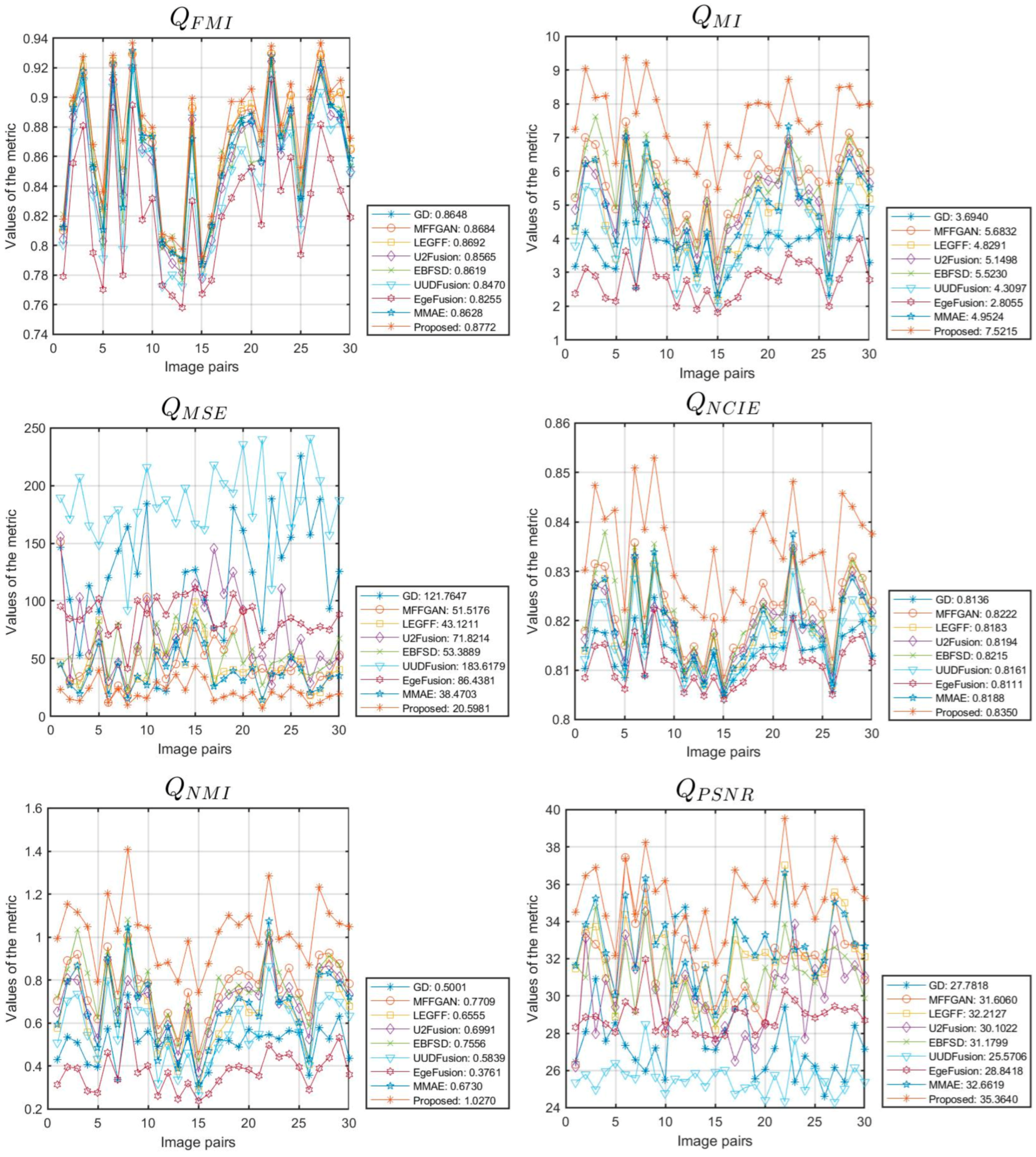
| GD | 0.6752 | 0.6301 | 105.0418 | 0.7754 | 0.8648 | 3.6940 | 121.7647 | 0.8136 | 0.5001 | 27.7818 |
| MFFGAN | 0.6427 | 0.6329 | 45.6960 | 0.7826 | 0.8684 | 5.6832 | 51.5176 | 0.8222 | 0.7709 | 31.6060 |
| LEGFF | 0.6190 | 0.6060 | 71.1462 | 0.7067 | 0.8692 | 4.8291 | 43.1211 | 0.8183 | 0.6555 | 32.2127 |
| U2Fusion | 0.5502 | 0.5156 | 119.8639 | 0.6970 | 0.8565 | 5.1498 | 71.8214 | 0.8194 | 0.6991 | 30.1022 |
| EBFSD | 0.5485 | 0.6531 | 63.7060 | 0.6558 | 0.8619 | 5.5230 | 53.3889 | 0.8215 | 0.7556 | 31.1799 |
| UUDFusion | 0.4576 | 0.6376 | 69.0701 | 0.5364 | 0.8470 | 4.3097 | 183.6179 | 0.8161 | 0.5839 | 25.5706 |
| EgeFusion | 0.2874 | 0.3277 | 537.7216 | 0.3757 | 0.8255 | 2.8055 | 86.4381 | 0.8111 | 0.3761 | 28.8418 |
| MMAE | 0.5916 | 0.6813 | 54.5921 | 0.6834 | 0.8628 | 4.9524 | 38.4703 | 0.8188 | 0.6730 | 32.6619 |
| Proposed | 0.7199 | 0.7875 | 23.7432 | 0.8429 | 0.8772 | 7.5215 | 20.5981 | 0.8350 | 1.0270 | 35.3640 |
Disclaimer/Publisher’s Note: The statements, opinions and data contained in all publications are solely those of the individual author(s) and contributor(s) and not of MDPI and/or the editor(s). MDPI and/or the editor(s) disclaim responsibility for any injury to people or property resulting from any ideas, methods, instructions or products referred to in the content. |
© 2025 by the authors. Licensee MDPI, Basel, Switzerland. This article is an open access article distributed under the terms and conditions of the Creative Commons Attribution (CC BY) license (https://creativecommons.org/licenses/by/4.0/).
Share and Cite
Li, L.; Song, S.; Lv, M.; Jia, Z.; Ma, H. Multi-Focus Image Fusion Based on Fractal Dimension and Parameter Adaptive Unit-Linking Dual-Channel PCNN in Curvelet Transform Domain. Fractal Fract. 2025, 9, 157. https://doi.org/10.3390/fractalfract9030157
Li L, Song S, Lv M, Jia Z, Ma H. Multi-Focus Image Fusion Based on Fractal Dimension and Parameter Adaptive Unit-Linking Dual-Channel PCNN in Curvelet Transform Domain. Fractal and Fractional. 2025; 9(3):157. https://doi.org/10.3390/fractalfract9030157
Chicago/Turabian StyleLi, Liangliang, Sensen Song, Ming Lv, Zhenhong Jia, and Hongbing Ma. 2025. "Multi-Focus Image Fusion Based on Fractal Dimension and Parameter Adaptive Unit-Linking Dual-Channel PCNN in Curvelet Transform Domain" Fractal and Fractional 9, no. 3: 157. https://doi.org/10.3390/fractalfract9030157
APA StyleLi, L., Song, S., Lv, M., Jia, Z., & Ma, H. (2025). Multi-Focus Image Fusion Based on Fractal Dimension and Parameter Adaptive Unit-Linking Dual-Channel PCNN in Curvelet Transform Domain. Fractal and Fractional, 9(3), 157. https://doi.org/10.3390/fractalfract9030157