Qualitative Analysis of Generalized Power Nonlocal Fractional System with p-Laplacian Operator, Including Symmetric Cases: Application to a Hepatitis B Virus Model

Abstract

This paper introduces a novel framework for modeling nonlocal fractional system with a p-Laplacian operator under power nonlocal fractional derivatives (PFDs), a generalization encompassing established derivatives like Caputo–Fabrizio, Atangana–Baleanu, weighted Atangana–Baleanu, and weighted Hattaf. The core methodology involves employing a PFD with a tunable power parameter within a non-singular kernel, enabling a nuanced representation of memory effects not achievable with traditional fixed-kernel derivatives. This flexible framework is analyzed using fixed-point theory, rigorously establishing the existence and uniqueness of solutions for four symmetric cases under specific conditions. Furthermore, we demonstrate the Hyers–Ulam stability, confirming the robustness of these solutions against small perturbations. The versatility and generalizability of this framework is underscored by its application to an epidemiological model of transmission of Hepatitis B Virus (HBV) and numerical simulations for all four symmetric cases. This study presents findings in both theoretical and applied aspects of fractional calculus, introducing an alternative framework for modeling complex systems with memory processes, offering opportunities for more sophisticated and accurate models and new avenues for research in fractional calculus and its applications.

1. Introduction

The study of dynamical systems is fundamental to understanding a wide array of phenomena across diverse fields of science and engineering. These systems, characterized by their evolving states, are often modeled using differential Equations [1,2,3,4]. While traditional integer-order differential equations have served as the cornerstone for many of these models, they can sometimes fall short when dealing with complex phenomena that exhibit memory effects and nonlocal interactions. In recent years, it has become increasingly evident that many real-world processes do not adhere to the assumptions underpinning classical integer-order models. Instead, their past trajectories influence their present states, leading to what is known as nonlocal behavior. To address this limitation, fractional calculus has emerged as a powerful mathematical tool. By extending the concept of differentiation and integration to non-integer orders, fractional derivatives offer a more versatile way to capture the memory and nonlocal characteristics inherent in many complex systems [5,6]. These advancements have driven extensive research toward the development of rigorous mathematical frameworks for fractional differential equations, particularly focusing on the existence and uniqueness conditions of their solutions, as well as the analysis of complex operators [7,8,9,10,11].

Among the more intriguing areas of research in this domain is the study of hybrid fractional differential equations. These equations are of particular importance since they integrate different types of fractional derivatives and operators, leading to richer and more accurate representations of complex systems [12,13,14]. A notable operator that often appears in hybrid fractional differential equations is the p-Laplacian operator. With applications in non-Newtonian fluid mechanics, image processing, and porous media flow, the inclusion of the p-Laplacian operator adds a layer of complexity and practical relevance [15,16,17]. However, the combination of a p-Laplacian operator with recent advancements in fractional calculus, such as PFD, still remains largely unexplored in the literature.

A novel class of nonlocal fractional derivatives, known as power fractional derivative (PFD), has recently been introduced based on the generalized power Mittag–Leffler (PML) function [18]. This operator generalizes existing derivatives, including Caputo–Fabrizio [19], Atangana–Baleanu [20], weighted Atangana–Baleanu [21], and Hattaf derivatives [22]. The key feature of PFD is its incorporation of a tunable power parameter “p”, enhancing flexibility in modeling diverse memory effects. This represents a significant advance beyond traditional fractional derivatives with fixed kernels. Prior research on PFD has primarily focused on establishing their basic properties, deriving their Laplace transform, and applying them to linear FDEs [18]. Recently, Zitane et al. [23] have investigated the existence, uniqueness, and numerical approximations for a class of fractional differential equations employing power nonlocal and non-singular kernels, the analysis of nonlinear fractional differential equations using PFD still lacks thorough investigations.

This work introduces a novel framework for modeling nonlocal fractional systems by combining a p-Laplacian operator with PFD. While individual studies of p-Laplacian operators with different fractional derivatives are present in the literature, their combination in a nonlinear system with PFD remains unexplored. Our work is one of the first to address this gap, allowing the study of a new class of problems and opening new avenues for more precise models of complex systems. The core novelty of our methodology lies in the use of a PFD with a tunable power parameter within a non-singular kernel, which allows for a more nuanced representation of memory effects than traditional fixed-kernel derivatives. This framework offers the possibility of more precise and flexible modeling of phenomena that cannot be described with traditional derivatives.

The PFD used in this work is distinct from many traditional fractional derivatives, such as those of Riemann–Liouville or Caputo, in it incorporates a ’power’ parameter within a non-singular kernel. This parameter provides additional flexibility in the way memory effects are modeled. The PFD is also a unifying concept that encompasses well-known derivatives as specific cases, such as Caputo–Fabrizio, Atangana–Baleanu, weighted Atangana–Baleanu, and weighted Hattaf. This means that different specific behaviors can be analyzed from the same, general definition, showing the great power of this framework. This ability to adapt the derivative to different modeling needs is a significant advantage compared with other, fixed-kernel derivatives.

The importance of developing new mathematical frameworks in fractional calculus that can model complex phenomena exhibiting memory effects and nonlocal interactions is evident in numerous fields of science and engineering. Such systems are commonly present in disease transmission, porous media flow, non-Newtonian fluid mechanics, and more. Accurate modeling is fundamental for creating better predictive models and control strategies in those fields. The combination of a PFD with p-Laplacian operators in our system offers opportunities for a new understanding of those systems, potentially yielding new ways of modeling and analyzing them. This work makes a significant contribution by providing an alternative and versatile framework for modeling those complex systems.

Significant efforts have been made in the field of fractional calculus in recent years. However, those works have focused on p-Laplacian operators within different fractional derivatives [24,25,26,27]. Our work contributes to the field of fractional calculus by combining the flexibility of PFD with the complexity of the p-Laplacian operator, thus filling a significant gap in the literature. In particular, our study of nonlinear fractional differential equations within this framework provides a significant contribution to the field. The proposed framework also contributes to the literature by providing the theoretical basis for numerical simulations using PFD in nonlinear systems, showing that these derivatives can be used in a similar way as other fractional order derivatives.

Motivated by these advancements, this article introduces a system of FDEs that features a p-Laplacian operator within a power nonlocal kernel. The primary objective is to provide a rigorous theoretical framework and enable numerical simulations for the following system

$$\left\{\begin{array}{c}{}_{a\hspace{1em}}{}^{\mathbb{PC}}\mathbf{D}_{\varsigma ,w}^{{\beta }_1,{\delta }_1,p}\left[{\phi }_{\theta }\left({}_{a\hspace{1em}}{}^{\mathbb{PC}}\mathbf{D}_{\varsigma ,w}^{{\beta }_2,{\delta }_2,p}\left(\mathbb{Y}\left(\varsigma \right)-\mathbb{F}\left(\varsigma ,\mathbb{Y}\left(\varsigma \right)\right)\right)\right)\right]=\mathbb{K}\left(\varsigma ,\mathbb{Y}\left(\varsigma \right)\right),\varsigma \in \left[a,b\right],a>0,\hfill \\ \mathbb{Y}\left(a\right)={\mathbb{Y}}_a,\hfill \end{array}\right.$$

(1)

where ${}_{a\hspace{1em}}{}^{\mathbb{PC}}\mathbf{D}_{\varsigma ,w}^{{\beta }_1,{\delta }_2,p}$ and ${}_{a\hspace{1em}}{}^{\mathbb{PC}}\mathbf{D}_{\varsigma ,w}^{{\beta }_1,{\delta }_2,p}$ are the PFD of order ${\beta }_1,{\beta }_2\in \left[0,1\right)$, in the Caputo sense, with respect to the non-decreasing weight function $w,$ min$\left({\delta }_1,{\delta }_2,p\right)>0,$ and the function $\mathbb{Y}\in H^1\left(a,b\right)$. The nonlinear functions $\mathbb{F},\mathbb{K}:\left[a,b\right]\times \mathbb{R}\to \mathbb{R}$ are continuous satisfies some conditions described later. The nonlinear operator ${\phi }_{\theta }\left(\chi \right)={\left|\chi \right|}^{\theta -2}\chi$$1<\theta <2$ and ${\displaystyle \frac{1}{\theta }}+{\displaystyle \frac{1}{q}}=1.$ The model (1) is generalized of many models depending on the parameters ${\beta }_1,{\delta }_1,{\beta }_2,{\delta }_2,p,$ and weighted function $w\left(\varsigma \right).$ The symmetric cases of model (1) are given as follows:

• If $p=e.$ Then, the model (1) is reduced to the weighted generalized Hattaf fractional model.
• If ${\delta }_1={\beta }_1,{\delta }_2={\beta }_2,$$p=e$ and $w\left(\varsigma \right)=1.$ Then, the model (1) is reduced to the Atangana–Baleanu fractional model.
• If ${\delta }_1={\beta }_1,{\delta }_2={\beta }_2,$$p=e.$ Then, the model (1) is reduced to the weighted Atangana–Baleanu fractional model.
• If ${\delta }_1={\delta }_2=1,$$p=e$ and $w\left(\varsigma \right)=1.$ Then, the model (1) is reduced to the Caputo–Fabrizio fractional model.

In this work, we develop a general framework, allowing to incorporation of a tunable power parameter. This framework is analyzed using fixed point theory. We establish the existence, uniqueness, and Hyers–Ulam stability of solutions as well as the existence, uniqueness and stability of solutions for four symmetric cases under specified conditions. Furthermore, to highlight the versatility and generalizability of our results, we apply the model to an epidemiological problem modeling the transmission of the Hepatitis B Virus (HBV). Numerical simulations for four distinct symmetric cases arising from our novel framework are presented to illustrate the applicability of our approach. This research contributes to the field of fractional calculus by

• Presenting a rigorous analysis of the existence and uniqueness of solutions for nonlinear hybrid fractional differential equations using a novel PFD within a p-Laplacian context which has not been extensively studied.
• Offering a generalized model that encompasses several existing formulations by varying a tuning power parameter.
• Demonstrating the Hyers–Ulam stability of the proposed model, indicating the robustness of the solutions under small perturbations.
• Providing numerical simulations for a range of cases and showing the application of the model to a real-world application through a complex disease transmission model.
• Ultimately, our findings provide an alternative framework for modeling complex systems with memory processes, creating opportunities for more sophisticated and accurate modeling tools and new avenues for research into the applications of fractional calculus.

By addressing both the theoretical aspects and the practical need for numerical solutions, this research significantly advances the field of fractional calculus and paves the way for wider application of PFD in modeling and analyzing complex real-world phenomena. This contribution is particularly important given the increasing recognition of the PFD’s versatility and potential in capturing the intricate dynamics of systems with memory effects.

2. Basic Concepts

To establish a basis for our subsequent analysis, this section introduces essential concepts concerning fractional operators characterized by power nonlocal and non-singular kernels. In 2022, Lotfi et al. [18] explored and defined the power fractional derivative, a new development in fractional calculus.

Definition 1

([18]). Let $\beta \in \left[0,1\right),$ with $\delta ,p>0,$ and $\mathbb{Y}\in H^1\left(a,b\right),$ where $H^1\left(a,b\right)$ is Sobolev space. The PFD of order β, in the Caputo sense, of a function $\mathbb{Y}$ with respect to the weight function $w,$$0<w\in C^1\left(\left[a,b\right]\right)$, is defined by

$${}_{a\hspace{1em}}{}^{\mathbb{PC}}\mathbf{D}_{\varsigma ,w}^{\beta ,\delta ,p}\mathbb{Y}\left(\varsigma \right)={\displaystyle \frac{\mathbb{PC}\left(\beta \right)}{1-\beta }}{\displaystyle \frac{1}{w\left(\varsigma \right)}}{\int }_a^{\varsigma }{}^p\mathbb{E}_{\delta ,1}\left(-{\displaystyle \frac{\beta }{1-\beta }}{\left(\varsigma -s\right)}^{\delta }\right){\left(w\mathbb{Y}\right)}^{\prime }\left(s\right)ds,$$

(2)

where

• ${}^p\mathbb{E}_{\delta ,l}$ represents the PML function given by

  $${}^p\mathbb{E}_{\delta ,l}\left(s\right)=\sum _{n=0}^{+\infty }{\displaystyle \frac{{\left(slnp\right)}^n}{\Gamma \left(kn+l\right)}},s\in \mathbb{C},and k,l,p>0.$$
• $\mathbb{PC}\left(\beta \right)$ represents a normalization positive function obeying $\mathbb{PC}\left(0\right)=\mathbb{PC}\left(1\right)=1.$

According to Theorem 1 of [18], the PML function ${}^p\mathbb{E}_{\delta ,l}\left(s\right)$ is locally uniformly convergent for any $s\in \mathbb{C},$ see Theorem 1 of [18].

Remark 1.

The PFD in the Caputo sense, as defined by Definition 1, serves as a generalization encompassing several well-established fractional derivatives. Specific cases of the PFD, obtained by particular choices of parameters, include

(1) Caputo–Fabrizio Fractional Derivative: If $w\left(\varsigma \right)=1$, $p=e$, and $\delta =1$, then Definition 1 reduces to the Caputo–Fabrizio fractional derivative:

$${}_{a\hspace{1em}}{}^{\mathbb{PC}}\mathbf{D}_{\varsigma ,1}^{\beta ,1,e}\mathbb{Y}\left(\varsigma \right)={\displaystyle \frac{\mathbb{PC}\left(\beta \right)}{1-\beta }}{\int }_a^{\varsigma }exp\left(-{\displaystyle \frac{\beta }{1-\beta }}\left(\varsigma -s\right)\right){\mathbb{Y}}^{\prime }\left(s\right)ds.$$

(2) Atangana–Baleanu Fractional Derivative: If $w\left(\varsigma \right)=1$, $p=e$, and $\beta =\delta$, then Definition 1 reduces to the Atangana–Baleanu fractional derivative:

$${}_{a\hspace{1em}}{}^{\mathbb{PC}}\mathbf{D}_{\varsigma ,1}^{\beta ,\beta ,e}\mathbb{Y}\left(\varsigma \right)={\displaystyle \frac{\mathbb{PC}\left(\beta \right)}{1-\beta }}{\int }_a^{\varsigma }{}^e\mathbb{E}_{\beta ,1}\left(-{\displaystyle \frac{\beta }{1-\beta }}{\left(\varsigma -s\right)}^{\beta }\right){\mathbb{Y}}^{\prime }\left(s\right)ds.$$

(3) Weighted Atangana–Baleanu Fractional Derivative: If $p=e$ and $\beta =\delta$, then Definition 1 reduces to the weighted Atangana–Baleanu fractional derivative:

$${}_{a\hspace{1em}}{}^{\mathbb{PC}}\mathbf{D}_{\varsigma ,w}^{\beta ,\beta ,e}\mathbb{Y}\left(\varsigma \right)={\displaystyle \frac{\mathbb{PC}\left(\beta \right)}{1-\beta }}{\displaystyle \frac{1}{w\left(\varsigma \right)}}{\int }_a^{\varsigma }{}^e\mathbb{E}_{\beta ,1}\left(-{\displaystyle \frac{\beta }{1-\beta }}{\left(\varsigma -s\right)}^{\beta }\right){\left(w\mathbb{Y}\right)}^{\prime }\left(s\right)ds.$$

(4) Weighted Generalized Hattaf Fractional Derivative: If $p=e$, then Definition 1 reduces to the weighted generalized Hattaf fractional derivative:

$${}_{a\hspace{1em}}{}^{\mathbb{PC}}\mathbf{D}_{\varsigma ,w}^{\beta ,\delta ,e}\mathbb{Y}\left(\varsigma \right)={\displaystyle \frac{\mathbb{PC}\left(\beta \right)}{1-\beta }}{\displaystyle \frac{1}{w\left(\varsigma \right)}}{\int }_a^{\varsigma }{}^e\mathbb{E}_{\delta ,1}\left(-{\displaystyle \frac{\beta }{1-\beta }}{\left(\varsigma -s\right)}^{\delta }\right){\left(w\mathbb{Y}\right)}^{\prime }\left(s\right)ds.$$

Definition 2

([18]). The PFI of order β, of a function $\mathbb{Y}$ with respect to the weight function $w,$$0<w\in C^1\left(\left[a,b\right]\right)$, is defined by

$${}_{a\hspace{1em}}{}^{\mathbb{PC}}\mathbf{I}_{\varsigma ,w}^{\beta ,\delta ,p}\mathbb{Y}\left(\varsigma \right)={\displaystyle \frac{1-\beta }{\mathbb{PC}\left(\beta \right)}}\mathbb{Y}\left(\varsigma \right)+lnp{{\displaystyle \frac{\beta }{\mathbb{PC}\left(\beta \right)}}}^{\mathbb{RL}}{\mathbf{I}}_{a,w}^{\delta }\mathbb{Y}\left(\varsigma \right),$$

where

• ${}^{\mathbb{RL}}\mathbf{I}_{a,w}^{\delta }\mathbb{Y}\left(\varsigma \right)$ denotes the standard weighted Riemann–Liouville fractional integral of order δ given by

  $${}^{\mathbb{RL}}\mathbf{I}_{a,w}^{\delta }\mathbb{Y}\left(\varsigma \right)={\displaystyle \frac{1}{\Gamma \left(\delta \right)}}{\displaystyle \frac{1}{w\left(\varsigma \right)}}{\int }_a^{\varsigma }{\left(\varsigma -s\right)}^{\delta -1}\left(w\mathbb{Y}\right)\left(s\right)ds.$$

Remark 2.

The Formula (2) can be expressed as follows:

$${}_{a\hspace{1em}}{}^{\mathbb{PC}}\mathbf{D}_{\varsigma ,w}^{\beta ,\delta ,p}\mathbb{Y}\left(\varsigma \right)={\displaystyle \frac{\mathbb{PC}\left(\beta \right)}{1-\beta }}\sum _{n=0}^{+\infty }{\left(-{\displaystyle \frac{\beta }{1-\beta }}{\left(\varsigma -s\right)}^{\delta }\right)}^n{}^{\mathbb{PC}}\mathbf{I}_{a,w}^{\delta n+1}\left({\displaystyle \frac{{\left(w\mathbb{Y}\right)}^{\prime }}{w}}\right)\left(\varsigma \right),$$

where the series converges locally and uniformly in $\varsigma .$

Theorem 1

(Theorem 1. [28]). Let $\beta \in \left[0,1\right),$ with $\delta ,p>0,$ and $\mathbb{Y}\in H^1\left(a,b\right).$ Then, the PFD and PFI are commutative operators as follows:

(i)

${}_{a\hspace{1em}}{}^{\mathbb{PC}}\mathbf{D}_{\varsigma ,w}^{\beta ,\delta ,p}\left({}_{a\hspace{1em}}{}^{\mathbb{PC}}\mathbf{I}_{\varsigma ,w}^{\beta ,\delta ,p}\mathbb{Y}\right)\left(\varsigma \right)=\mathbb{Y}\left(\varsigma \right)-{\displaystyle \frac{w\mathbb{Y}\left(a\right)}{w\left(\varsigma \right)}};$

(ii)

${}_{a\hspace{1em}}{}^{\mathbb{PC}}\mathbf{I}_{\varsigma ,w}^{\beta ,\delta ,p}\left({}_{a\hspace{1em}}{}^{\mathbb{PC}}\mathbf{D}_{\varsigma ,w}^{\beta ,\delta ,p}\mathbb{Y}\right)\left(\varsigma \right)=\mathbb{Y}\left(\varsigma \right)-{\displaystyle \frac{w\mathbb{Y}\left(a\right)}{w\left(\varsigma \right)}}.$

If we put $p=e$, then we obtain the results of generalized Hattaf fractional operators [29].

Lemma 1.

The PFD and PFI satisfy the Newton–Leibniz formula

$${}_{a\hspace{1em}}{}^{\mathbb{PC}}\mathbf{D}_{\varsigma ,w}^{\beta ,\delta ,p}\left({}_{a\hspace{1em}}{}^{\mathbb{PC}}\mathbf{I}_{\varsigma ,w}^{\beta ,\delta ,p}\mathbb{Y}\right)\left(\varsigma \right){=}_a^{\mathbb{PC}}{\mathbf{I}}_{\varsigma ,w}^{\beta ,\delta ,p}\left({}_{a\hspace{1em}}{}^{\mathbb{PC}}\mathbf{D}_{\varsigma ,w}^{\beta ,\delta ,p}\mathbb{Y}\right)\left(\varsigma \right)=\mathbb{Y}\left(\varsigma \right)-\mathbb{Y}\left(a\right).$$

Lemma 2

([30,31]). Let ${\phi }_{\theta }$ be a $\theta -$Laplacian operator. Then, the following conditions hold true:

(1) For $1<\theta \le 2,{\mathbb{X}}_1,{\mathbb{X}}_2>0,$ and $\left|{\mathbb{X}}_1\right|,\left|{\mathbb{X}}_2\right|\ge \xi >0,$ we have

$$\left|{\phi }_{\theta }\left({\mathbb{X}}_1\right)-{\phi }_{\theta }\left({\mathbb{X}}_2\right)\right|\le \left(\theta -1\right){\xi }^{\theta -2}\left|{\mathbb{X}}_1-{\mathbb{X}}_2\right|.$$

(2) For $\theta >1,$ and $\left|{\mathbb{X}}_1\right|,\left|{\mathbb{X}}_2\right|\le {\xi }^{*}>0,$ we have

$$\left|{\phi }_{\theta }\left({\mathbb{X}}_1\right)-{\phi }_{\theta }\left({\mathbb{X}}_2\right)\right|\le \left(\theta -1\right){\left({\xi }^{*}\right)}^{\theta -2}\left|{\mathbb{X}}_1-{\mathbb{X}}_2\right|.$$

Lemma 3

([28]). Let $\mathbb{K}:\left[0,1\right]\times \mathbb{R}\to \mathbb{R}$ be a continuous nonlinear function such that $\mathbb{K}\left(a,\mathbb{Y}\left(a\right)\right)=0.$ Then, the function $\mathbb{Y}\in C\left(\left[a,b\right]\right)$ is a solution of the following problem

$$\left\{\begin{array}{c}{}_{a\hspace{1em}}{}^{\mathbb{PC}}\mathbf{D}_{\varsigma ,w}^{\beta ,\delta ,p}\mathbb{Y}\left(\varsigma \right)=\mathbb{K}\left(\varsigma ,\mathbb{Y}\left(\varsigma \right)\right),\\ \mathbb{Y}\left(0\right)={\mathbb{Y}}_a\in \mathbb{R},\end{array}\right.$$

if and only if $\mathbb{Y}$ satisfies the following integral equation

$$\mathbb{Y}\left(\varsigma \right)={\displaystyle \frac{w\left(a\right)}{w\left(\varsigma \right)}}{\mathbb{Y}}_a{+}_a^{\mathbb{PC}}{\mathbf{I}}_{\varsigma ,w}^{\beta ,\delta ,p}\mathbb{K}\left(\varsigma ,\mathbb{Y}\left(\varsigma \right)\right).$$

Definition 3.

Assume $\mathbb{G}:\mathcal{N}\subset \mathbb{Q}\to \mathbb{Q}$ is a bounded and continuous operator. Then, the operator $\mathbb{G}$ is Lipschitz with a Lipschitz constant Υ, provided

$$∥\mathbb{G}\left(u\right)-\mathbb{G}\left(\widehat{u}\right)∥\le {\rm Y}∥u-\widehat{u}∥,{\rm Y}>0,$$

for all $u,\widehat{u}\in \mathcal{N}$. Furthermore, the operator $\mathbb{G}$ is classified as a strict contraction provided ${\rm Y}<1.$

Proposition 1.

The operator $\mathbb{G}:\mathcal{N}\to \mathbb{Q}$ is satisfies the property of being Υ–Lipschitz with constants equal to 0 if $\mathbb{G}$ is compact.

Hypothesis

We impose the following assumptions for our analysis of existence, uniqueness, and stability

$\left(H_1\right)$ For the continuous functions $\mathbb{K}$ and $\mathbb{F}$, there exists constant number ${\mathbb{L}}_{\mathbb{K}},{\mathbb{L}}_{\mathbb{F}}>0$ such that

$$\left|\mathbb{K}\left(\varsigma ,\mathbb{Y}\left(\varsigma \right)\right)-\mathbb{K}\left(\varsigma ,\widehat{\mathbb{Y}}\left(\varsigma \right)\right)\right|\le {\mathbb{L}}_{\mathbb{K}}\left|\mathbb{Y}\left(\varsigma \right)-\widehat{\mathbb{Y}}\left(\varsigma \right)\right|,for\varsigma \in \mathcal{J},$$

and

$$\mathbb{F}\left(\varsigma ,\mathbb{Y}\left(\varsigma \right)\right)-\mathbb{F}\left(\varsigma ,\widehat{\mathbb{Y}}\left(\varsigma \right)\right)\le {\mathbb{L}}_{\mathbb{F}}\left|\mathbb{Y}\left(\varsigma \right)-\widehat{\mathbb{Y}}\left(\varsigma \right)\right|,for\varsigma \in \mathcal{J}.$$

$\left(H_2\right)$ The functions $\mathbb{K},\Psi$ are continuous and there exist constants ${\lambda }_{\mathbb{K}},{\eta }_{\mathbb{K}}>0,$ and ${\lambda }_{\mathbb{F}},{\eta }_{\mathbb{F}}$ such that

$$\left|\mathbb{K}\left(\varsigma ,\mathbb{Y}\left(\varsigma \right)\right)\right|\le {\lambda }_{\mathbb{K}}+\left|\mathbb{Y}\left(\varsigma \right)\right|{\eta }_{\mathbb{K}},for\varsigma \in \mathcal{J},$$

and

$$\left|\mathbb{F}\left(\varsigma ,\mathbb{Y}\left(\varsigma \right)\right)\right|\le {\lambda }_{\mathbb{F}}+\left|\mathbb{Y}\left(\varsigma \right)\right|{\eta }_{\mathbb{F}},for\varsigma \in \mathcal{J}.$$

3. Qualitative Behavior of the Power Nonlocal Model (1) with p-Laplacian Operator

3.1. Equivalent Integral Equation

In the following theorem, we convert the power nonlocal model (1) with p-Laplacian operator into equivalent integral equations.

Theorem 2.

The solution of model (1) is given by

$$\begin{array}{ccc}\hfill \mathbb{Y}\left(\varsigma \right)& =& {\displaystyle \frac{w\left(a\right)}{w\left(\varsigma \right)}}{\mathbb{Y}}_a+\mathbb{F}\left(\varsigma ,\mathbb{Y}\left(\varsigma \right)\right)+{\phi }_q{\displaystyle \frac{\left(1-{\beta }_2\right)\left(1-{\beta }_1\right)}{\mathbb{PC}\left({\beta }_2\right)\mathbb{PC}\left({\beta }_1\right)}}\mathbb{K}\left(\varsigma ,\mathbb{Y}\left(\varsigma \right)\right)\hfill \\ & & +{\displaystyle \frac{{\phi }_q\left(lnp\right){\beta }_1\left(1-{\beta }_2\right)}{\mathbb{PC}\left({\beta }_1\right)\mathbb{PC}\left({\beta }_2\right)\Gamma \left({\delta }_1\right)w\left(\varsigma \right)}}{\int }_a^{\varsigma }{\left(\varsigma -s\right)}^{{\delta }_1-1}\left(w\mathbb{K}\left(s,\mathbb{Y}\left(s\right)\right)\right)ds\hfill \\ & & +{\displaystyle \frac{\left(lnp\right){\beta }_2\left(1-{\beta }_1\right)}{\mathbb{PC}\left({\beta }_2\right)\mathbb{PC}\left({\beta }_1\right)\Gamma \left({\delta }_2\right)w\left(\varsigma \right)}}{\int }_a^{\varsigma }{\left(\varsigma -s\right)}^{{\delta }_2-1}{\phi }_q\left(w\mathbb{K}\left(s,\mathbb{Y}\left(s\right)\right)\right)ds\hfill \\ & & +{\displaystyle \frac{{\left(lnp\right)}^2{\beta }_2{\beta }_1}{\mathbb{PC}\left({\beta }_2\right)\mathbb{PC}\left({\beta }_1\right)\Gamma ({\delta }_1+{\delta }_2)w\left(\varsigma \right)}}{\int }_a^{\varsigma }{\left(\varsigma -s\right)}^{{\delta }_1+{\delta }_2-1}{\phi }_q\left(w\mathbb{K}\left(s,\mathbb{Y}\left(s\right)\right)\right)ds.\hfill \end{array}$$

Proof. 

Apply ${}_{a\hspace{1em}}{}^{\mathbb{PC}}\mathbf{I}_{\varsigma ,w}^{{\beta }_1,{\delta }_1,p}$ to the system (1), we have

$${}_{a\hspace{1em}}{}^{\mathbb{PC}}\mathbf{I}_{\varsigma ,w}^{{\beta }_1,{\delta }_1,p}\left({}_{a\hspace{1em}}{}^{\mathbb{PC}}\mathbf{D}_{\varsigma ,w}^{{\beta }_1,{\delta }_1,p}\left[{\phi }_{\theta }\left({}_{a\hspace{1em}}{}^{\mathbb{PC}}\mathbf{D}_{\varsigma ,w}^{{\beta }_2,{\delta }_2,p}\left(\mathbb{Y}\left(\varsigma \right)-\mathbb{F}\left(\varsigma ,\mathbb{Y}\left(\varsigma \right)\right)\right)\right)\right]\right){=}_a^{\mathbb{PC}}{\mathbf{I}}_{\varsigma ,w}^{{\beta }_1,{\delta }_1,p}\mathbb{K}\left(\varsigma ,\mathbb{Y}\left(\varsigma \right)\right).$$

By Def 2 and Theorem 1, we have

$$\begin{array}{ccc}\hfill {\phi }_{\theta }\left({}_{a\hspace{1em}}{}^{\mathbb{PC}}\mathbf{D}_{\varsigma ,w}^{{\beta }_2,{\delta }_2,p}\left(\mathbb{Y}\left(\varsigma \right)-\mathbb{F}\left(\varsigma ,\mathbb{Y}\left(\varsigma \right)\right)\right)\right)& =& {\displaystyle \frac{w\left(a\right){\left.{\phi }_{\theta }{}_{a\hspace{1em}}{}^{\mathbb{PC}}\mathbf{D}_{\varsigma ,w}^{{\beta }_2,{\delta }_2,p}\left(\mathbb{Y}\left(\varsigma \right)-\mathbb{F}\left(\varsigma ,\mathbb{Y}\left(\varsigma \right)\right)\right)\right|}_{\varsigma =a}}{w\left(\varsigma \right)}}\hfill \\ & & +{}_{a\hspace{1em}}{}^{\mathbb{PC}}\mathbf{I}_{\varsigma ,w}^{{\beta }_1,{\delta }_1,p}\mathbb{K}\left(\varsigma ,\mathbb{Y}\left(\varsigma \right)\right).\hfill \end{array}$$

This implies that

$${\phi }_{\theta }\left({}_{a\hspace{1em}}{}^{\mathbb{PC}}\mathbf{D}_{\varsigma ,w}^{{\beta }_2,{\delta }_2,p}\left(\mathbb{Y}\left(\varsigma \right)-\mathbb{F}\left(\varsigma ,\mathbb{Y}\left(\varsigma \right)\right)\right)\right){=}_a^{\mathbb{PC}}{\mathbf{I}}_{\varsigma ,w}^{{\beta }_1,{\delta }_1,p}\mathbb{K}\left(\varsigma ,\mathbb{Y}\left(\varsigma \right)\right).$$

By the p-Laplacian operator, we have

$${}_{a\hspace{1em}}{}^{\mathbb{PC}}\mathbf{D}_{\varsigma ,w}^{{\beta }_2,{\delta }_2,p}\left(\mathbb{Y}\left(\varsigma \right)-\mathbb{F}\left(\varsigma ,\mathbb{Y}\left(\varsigma \right)\right)\right)={\phi }_q\left({}_{a\hspace{1em}}{}^{\mathbb{PC}}\mathbf{I}_{\varsigma ,w}^{{\beta }_1,{\delta }_1,p}\mathbb{K}\left(\varsigma ,\mathbb{Y}\left(\varsigma \right)\right)\right).$$

Apply again ${}_{a\hspace{1em}}{}^{\mathbb{PC}}\mathbf{I}_{\varsigma ,w}^{{\beta }_2,{\delta }_2,p}$ to above equation, we obtain

$$\mathbb{Y}\left(\varsigma \right)-\mathbb{F}\left(\varsigma ,\mathbb{Y}\left(\varsigma \right)\right)={\displaystyle \frac{w\left(a\right)\left[\mathbb{Y}\left(a\right)-\mathbb{F}\left(a,\mathbb{Y}\left(a\right)\right)\right]}{w\left(\varsigma \right)}}{+}_a^{\mathbb{PC}}{\mathbf{I}}_{\varsigma ,w}^{{\beta }_2,{\delta }_2,p}{\phi }_q\left({}_{a\hspace{1em}}{}^{\mathbb{PC}}\mathbf{I}_{\varsigma ,w}^{{\beta }_1,{\delta }_1,p}\mathbb{K}\left(\varsigma ,\mathbb{Y}\left(\varsigma \right)\right)\right).$$

By conditions $\mathbb{Y}\left(a\right)={\mathbb{Y}}_a,$ and ${\left.\mathbb{F}\left(\varsigma ,\mathbb{X}\left(\varsigma \right)\right)\right|}_{\varsigma =a}=0,$ we have

$$\mathbb{Y}\left(\varsigma \right)={\displaystyle \frac{w\left(a\right)}{w\left(\varsigma \right)}}{\mathbb{Y}}_a+\mathbb{F}\left(\varsigma ,\mathbb{Y}\left(\varsigma \right)\right){+}_a^{\mathbb{PC}}{\mathbf{I}}_{\varsigma ,w}^{{\beta }_2,{\delta }_2,p}{\phi }_q\left({}_{a\hspace{1em}}{}^{\mathbb{PC}}\mathbf{I}_{\varsigma ,w}^{{\beta }_1,{\delta }_1,p}\mathbb{K}\left(\varsigma ,\mathbb{Y}\left(\varsigma \right)\right)\right).$$

By Theorem 1, we have

$$\begin{array}{ccc}\hfill \mathbb{Y}\left(\varsigma \right)& =& {\displaystyle \frac{w\left(a\right)}{w\left(\varsigma \right)}}{\mathbb{Y}}_a+\mathbb{F}\left(\varsigma ,\mathbb{Y}\left(\varsigma \right)\right){+}_a^{\mathbb{PC}}{\mathbf{I}}_{\varsigma ,w}^{{\beta }_2,{\delta }_2,p}{\phi }_q\left({\displaystyle \frac{1-{\beta }_1}{\mathbb{PC}\left({\beta }_1\right)}}\mathbb{K}\left(\varsigma ,\mathbb{Y}\left(\varsigma \right)\right)+lnp{{\displaystyle \frac{{\beta }_1}{\mathbb{PC}\left({\beta }_1\right)}}}^{\mathbb{RL}}{\mathbf{I}}_{a,w}^{{\delta }_1}\mathbb{K}\left(\varsigma ,\mathbb{Y}\left(\varsigma \right)\right)\right)\hfill \\ & =& {\mathbb{Y}}_a+\mathbb{F}\left(\varsigma ,\mathbb{Y}\left(\varsigma \right)\right)+{\phi }_q{\displaystyle \frac{1-{\beta }_2}{\mathbb{PC}\left({\beta }_2\right)}}\left({\displaystyle \frac{1-{\beta }_1}{\mathbb{PC}\left({\beta }_1\right)}}\mathbb{K}\left(\varsigma ,\mathbb{Y}\left(\varsigma \right)\right)+lnp{{\displaystyle \frac{{\beta }_1}{\mathbb{PC}\left({\beta }_1\right)}}}^{\mathbb{RL}}{\mathbf{I}}_{a,w}^{{\delta }_1}\mathbb{K}\left(\varsigma ,\mathbb{Y}\left(\varsigma \right)\right)\right)\hfill \\ & & +lnp{{\displaystyle \frac{{\beta }_2}{\mathbb{PC}\left({\beta }_2\right)}}}^{\mathbb{RL}}{\mathbf{I}}_{a,w}^{{\delta }_2}{\phi }_q\left({\displaystyle \frac{1-{\beta }_1}{\mathbb{PC}\left({\beta }_1\right)}}\mathbb{K}\left(\varsigma ,\mathbb{Y}\left(\varsigma \right)\right)+lnp{{\displaystyle \frac{{\beta }_1}{\mathbb{PC}\left({\beta }_1\right)}}}^{\mathbb{RL}}{\mathbf{I}}_{a,w}^{{\delta }_1}\mathbb{Y}\left(\varsigma ,\mathbb{X}\left(\varsigma \right)\right)\right)\hfill \\ & =& {\mathbb{Y}}_a+\mathbb{F}\left(\varsigma ,\mathbb{Y}\left(\varsigma \right)\right)+{\phi }_q{\displaystyle \frac{\left(1-{\beta }_2\right)\left(1-{\beta }_1\right)}{\mathbb{PC}\left({\beta }_2\right)\mathbb{PC}\left({\beta }_1\right)}}\mathbb{K}\left(\varsigma ,\mathbb{Y}\left(\varsigma \right)\right)\hfill \\ & & +{\displaystyle \frac{{\phi }_q\left(lnp\right){\beta }_1\left(1-{\beta }_2\right)}{\mathbb{PC}\left({\beta }_1\right)\mathbb{PC}\left({\beta }_2\right)\Gamma \left({\delta }_1\right)w\left(\varsigma \right)}}{\int }_a^{\varsigma }{\left(\varsigma -s\right)}^{{\delta }_1-1}\left(w\mathbb{K}\left(s,\mathbb{Y}\left(s\right)\right)\right)ds\hfill \\ & & +{\displaystyle \frac{\left(lnp\right){\beta }_2\left(1-{\beta }_1\right)}{\mathbb{PC}\left({\beta }_2\right)\mathbb{PC}\left({\beta }_1\right)\Gamma \left({\delta }_2\right)w\left(\varsigma \right)}}{\int }_a^{\varsigma }{\left(\varsigma -s\right)}^{{\delta }_2-1}{\phi }_q\left(w\mathbb{K}\left(s,\mathbb{Y}\left(s\right)\right)\right)ds\hfill \\ & & +{\displaystyle \frac{{\left(lnp\right)}^2{\beta }_2{\beta }_1}{\mathbb{PC}\left({\beta }_2\right)\mathbb{P}\underset{\square }{\mathbb{C}}\left({\beta }_1\right)\Gamma ({\delta }_1+{\delta }_2)w\left(\varsigma \right)}}{\int }_a^{\varsigma }{\left(\varsigma -s\right)}^{{\delta }_1+{\delta }_2-1}{\phi }_q\left(w\mathbb{K}\left(s,\mathbb{Y}\left(s\right)\right)\right)ds.\hfill \end{array}$$

To simplify our analysis, we rewrite the solution as follows

$$\begin{array}{ccc}\hfill \mathbb{Y}\left(\varsigma \right)& =& {\displaystyle \frac{w\left(a\right)}{w\left(\varsigma \right)}}{\mathbb{Y}}_a+\mathbb{F}\left(\varsigma ,\mathbb{Y}\left(\varsigma \right)\right)+{\phi }_q{\Psi }_1\left({\beta }_1,{\beta }_2\right)\mathbb{K}\left(\varsigma ,\mathbb{Y}\left(\varsigma \right)\right)\hfill \\ & & +{\displaystyle \frac{{\phi }_q\left(lnp\right){\Psi }_2\left({\beta }_1,{\beta }_2\right)}{\Gamma \left({\delta }_1\right)w\left(\varsigma \right)}}{\int }_a^{\varsigma }{\left(\varsigma -s\right)}^{{\delta }_1-1}\left(w\mathbb{K}\left(s,\mathbb{Y}\left(s\right)\right)\right)ds\hfill \\ & & +{\displaystyle \frac{\left(lnp\right){\Psi }_3\left({\beta }_1,{\beta }_2\right)}{\Gamma \left({\delta }_2\right)w\left(\varsigma \right)}}{\int }_a^{\varsigma }{\left(\varsigma -s\right)}^{{\delta }_2-1}{\phi }_q\left(w\mathbb{K}\left(s,\mathbb{Y}\left(s\right)\right)\right)ds\hfill \\ & & +{\displaystyle \frac{{\left(lnp\right)}^2{\Psi }_4\left({\beta }_1,{\beta }_2\right)}{\Gamma ({\delta }_1+{\delta }_2)w\left(\varsigma \right)}}{\int }_a^{\varsigma }{\left(\varsigma -s\right)}^{{\delta }_1+{\delta }_2-1}{\phi }_q\left(w\mathbb{K}\left(s,\mathbb{Y}\left(s\right)\right)\right)ds,\hfill \end{array}$$

where

$$\begin{array}{ccc}\hfill {\Psi }_1\left({\beta }_1,{\beta }_2\right)& =& {\displaystyle \frac{\left(1-{\beta }_2\right)\left(1-{\beta }_1\right)}{\mathbb{PC}\left({\beta }_2\right)\mathbb{PC}\left({\beta }_1\right)}},\hfill \\ \hfill {\Psi }_2\left({\beta }_1,{\beta }_2\right)& =& {\displaystyle \frac{{\beta }_1\left(1-{\beta }_2\right)}{\mathbb{PC}\left({\beta }_1\right)\mathbb{PC}\left({\beta }_2\right)}},\hfill \\ \hfill {\Psi }_3\left({\beta }_1,{\beta }_2\right)& =& {\displaystyle \frac{{\beta }_2\left(1-{\beta }_1\right)}{\mathbb{PC}\left({\beta }_2\right)\mathbb{PC}\left({\beta }_1\right)}},\hfill \\ \hfill {\Psi }_4\left({\beta }_1,{\beta }_2\right)& =& {\displaystyle \frac{{\beta }_2{\beta }_1}{\mathbb{PC}\left({\beta }_2\right)\mathbb{PC}\left({\beta }_1\right)}}.\hfill \end{array}$$

3.2. Notations

To prepare for our analysis, we establish the following notations.

$$\begin{array}{ccc}\hfill \mathcal{O}& =& \left(q-1\right){\xi }^{q-2}\left({\Psi }_1\left({\beta }_1,{\beta }_2\right)+\left(lnp\right){\Psi }_2\left({\beta }_1,{\beta }_2\right){\displaystyle \frac{{\left(b-a\right)}^{{\delta }_1}}{\Gamma \left({\delta }_1+1\right)}}\right.\hfill \\ & & +\left.\left(lnp\right){\Psi }_3\left({\beta }_1,{\beta }_2\right){\displaystyle \frac{{\left(b-a\right)}^{{\delta }_2}}{\Gamma \left({\delta }_2+1\right)}}+{\left(lnp\right)}^2{\Psi }_4\left({\beta }_1,{\beta }_2\right){\displaystyle \frac{{\left(b-a\right)}^{{\delta }_1+{\delta }_2}}{\Gamma \left({\delta }_1+{\delta }_2+1\right)}}\right),\hfill \end{array}$$

$${\rm Y}={\mathbb{L}}_{\mathbb{F}}+{\mathbb{L}}_{\mathbb{K}}\mathcal{O}.$$

By Theorem 2, we will define an operator $\mathbb{G}:\mathbb{Q}\to \mathbb{Q}$ by

$$\begin{array}{ccc}\hfill \mathbb{G}\left(\mathbb{Y}\left(\varsigma \right)\right)& =& {\displaystyle \frac{w\left(a\right)}{w\left(\varsigma \right)}}{\mathbb{Y}}_a+\mathbb{F}\left(\varsigma ,\mathbb{Y}\left(\varsigma \right)\right)+{\phi }_q{\Psi }_1\left({\beta }_1,{\beta }_2\right)\mathbb{K}\left(\varsigma ,\mathbb{Y}\left(\varsigma \right)\right)\hfill \\ & & +{\displaystyle \frac{{\phi }_{q}lnp{\Psi }_2\left({\beta }_1,{\beta }_2\right)}{\Gamma \left({\delta }_1\right)w\left(\varsigma \right)}}{\int }_a^{\varsigma }{\left(\varsigma -s\right)}^{{\delta }_1-1}\left(w\mathbb{K}\left(s,\mathbb{Y}\left(s\right)\right)\right)ds\hfill \\ & & +{\displaystyle \frac{lnp{\Psi }_3\left({\beta }_1,{\beta }_2\right)}{\Gamma \left({\delta }_2\right)w\left(\varsigma \right)}}{\int }_a^{\varsigma }{\left(\varsigma -s\right)}^{{\delta }_2-1}{\phi }_q\left(w\mathbb{K}\left(s,\mathbb{Y}\left(s\right)\right)\right)ds\hfill \\ & & +{\displaystyle \frac{{\left(lnp\right)}^2{\Psi }_4\left({\beta }_1,{\beta }_2\right)}{\Gamma ({\delta }_1+{\delta }_2)w\left(\varsigma \right)}}{\int }_a^{\varsigma }{\left(\varsigma -s\right)}^{{\delta }_1+{\delta }_2-1}{\phi }_q\left(w\mathbb{K}\left(s,\mathbb{Y}\left(s\right)\right)\right)ds.\hfill \end{array}$$

(3)

The model given by Equation (1) possesses a solution precisely when the operator $\mathbb{G}$ has fixed points.

3.3. Lipschitz Properties of Operator $\mathbb{G}$

Theorem 3.

Under assumptions ($H_1-H_3$), the operator $\mathbb{G}$ is Υ-Lipschitz, provided that ${\rm Y}<1.$

Proof. 

Let $\mathbb{Y},\widehat{\mathbb{Y}}\in \mathbb{Q}$. Then, for $\varsigma \in \left[a,b\right]$ we have

$$\begin{array}{ccc}& & \left|\mathbb{G}\left(\mathbb{Y}\left(\varsigma \right)\right)-\mathbb{G}\left(\widehat{\mathbb{Y}}\left(\varsigma \right)\right)\right|\hfill \\ & \le & \left|\mathbb{F}\left(\varsigma ,\mathbb{Y}\left(\varsigma \right)\right)-\mathbb{F}\left(\varsigma ,\widehat{\mathbb{Y}}\left(\varsigma \right)\right)\right|+{\Psi }_1\left({\beta }_1,{\beta }_2\right)\left|{\phi }_q\mathbb{K}\left(\varsigma ,\mathbb{Y}\left(\varsigma \right)\right)-{\phi }_q\mathbb{K}\left(\varsigma ,\widehat{\mathbb{Y}}\left(\varsigma \right)\right)\right|\hfill \\ & & +{\displaystyle \frac{{\phi }_{q}lnp{\Psi }_2\left({\beta }_1,{\beta }_2\right)}{\Gamma \left({\delta }_1\right)w\left(\varsigma \right)}}{\int }_a^{\varsigma }{\left(\varsigma -s\right)}^{{\delta }_1-1}\left(w\left|\mathbb{K}\left(s,\mathbb{Y}\left(s\right)\right)-\mathbb{K}\left(s,\widehat{\mathbb{Y}}\left(\varsigma s\right)\right)\right|\right)ds\hfill \\ & & +{\displaystyle \frac{lnp{\Psi }_3\left({\beta }_1,{\beta }_2\right)}{\Gamma \left({\delta }_2\right)w\left(\varsigma \right)}}{\int }_a^{\varsigma }{\left(\varsigma -s\right)}^{{\delta }_2-1}\left(w\left|{\phi }_q\mathbb{K}\left(s,\mathbb{Y}\left(s\right)\right)-{\phi }_q\mathbb{K}\left(s,\widehat{\mathbb{Y}}\left(\varsigma s\right)\right)\right|\right)ds\hfill \\ & & +{\displaystyle \frac{{\left(lnp\right)}^2{\Psi }_4\left({\beta }_1,{\beta }_2\right)}{\Gamma ({\delta }_1+{\delta }_2)w\left(\varsigma \right)}}{\int }_a^{\varsigma }{\left(\varsigma -s\right)}^{{\delta }_1+{\delta }_2-1}\left(w\left|{\phi }_q\mathbb{K}\left(s,\mathbb{Y}\left(s\right)\right)-{\phi }_q\mathbb{K}\left(s,\widehat{\mathbb{Y}}\left(\varsigma s\right)\right)\right|\right)ds.\hfill \end{array}$$

By (H₁) and (H₃), we have

$$\begin{array}{ccc}\hfill \left|\mathbb{G}\left(\mathbb{Y}\left(\varsigma \right)\right)-\mathbb{G}\left(\widehat{\mathbb{Y}}\left(\varsigma \right)\right)\right|& \le & {\mathbb{L}}_{\mathbb{F}}\left|\mathbb{Y}\left(\varsigma \right)-\widehat{\mathbb{Y}}\left(\varsigma \right)\right|+{\Psi }_1\left({\beta }_1,{\beta }_2\right)\left(q-1\right){\xi }^{q-2}{\mathbb{L}}_{\mathbb{K}}\left|\mathbb{Y}\left(\varsigma \right)-\widehat{\mathbb{Y}}\left(\varsigma \right)\right|\hfill \\ & & +\left(q-1\right){\xi }^{q-2}\left(lnp\right){\Psi }_2\left({\beta }_1,{\beta }_2\right){\displaystyle \frac{{\left(\varsigma -a\right)}^{{\delta }_1}}{\Gamma \left({\delta }_1+1\right)}}{\mathbb{L}}_{\mathbb{K}}\left|\mathbb{Y}\left(\varsigma \right)-\widehat{\mathbb{Y}}\left(\varsigma \right)\right|\hfill \\ & & +\left(q-1\right){\xi }^{q-2}\left(lnp\right){\Psi }_3\left({\beta }_1,{\beta }_2\right){\displaystyle \frac{{\left(\varsigma -a\right)}^{{\delta }_2}}{\Gamma \left({\delta }_2+1\right)}}{\mathbb{L}}_{\mathbb{K}}\left|\mathbb{Y}\left(\varsigma \right)-\widehat{\mathbb{Y}}\left(\varsigma \right)\right|\hfill \\ & & +\left(q-1\right){\xi }^{q-2}{\left(lnp\right)}^2{\Psi }_4\left({\beta }_1,{\beta }_2\right){\displaystyle \frac{{\left(\varsigma -a\right)}^{{\delta }_1+{\delta }_2}}{\Gamma \left({\delta }_1+{\delta }_2+1\right)}}{\mathbb{L}}_{\mathbb{K}}\left|\mathbb{Y}\left(\varsigma \right)-\widehat{\mathbb{Y}}\left(\varsigma \right)\right|.\hfill \end{array}$$

Thus, by (3), we have

$$\begin{array}{ccc}& & ∥\mathbb{G}\left(\mathbb{Y}\right)-\mathbb{G}\left(\widehat{\mathbb{Y}}\right)∥\hfill \\ & \le & \left[{\mathbb{L}}_{\mathbb{F}}+\left(q-1\right){\xi }^{q-2}{\mathbb{L}}_{\mathbb{K}}\left({\Psi }_1\left({\beta }_1,{\beta }_2\right)+{\displaystyle \frac{\left(lnp\right){\Psi }_2\left({\beta }_1,{\beta }_2\right){\left(b-a\right)}^{{\delta }_1}}{\Gamma \left({\delta }_1+1\right)}}\right.\right.\hfill \\ & & +\left.\left.{\displaystyle \frac{\left(lnp\right){\Psi }_3\left({\beta }_1,{\beta }_2\right){\left(b-a\right)}^{{\delta }_2}}{\Gamma \left({\delta }_2+1\right)}}+{\displaystyle \frac{{\left(lnp\right)}^2{\Psi }_4\left({\beta }_1,{\beta }_2\right){\left(b-a\right)}^{{\delta }_1+{\delta }_2}}{\Gamma \left({\delta }_1+{\delta }_2+1\right)}}\right)\right]∥\mathbb{Y}-\widehat{\mathbb{Y}}∥.\hfill \end{array}$$

(4)

Then, by (4) we getobtain

$$∥\mathbb{G}\left(\mathbb{Y}\right)-\mathbb{G}\left(\widehat{\mathbb{Y}}\right)∥\le {\rm Y}∥\mathbb{Y}-\widehat{\mathbb{Y}}∥.$$

Thus, $\mathbb{G}$ is ${\rm Y}$-Lipschitz. □

3.4. Compactness of Operator $\mathbb{G}$

Theorem 4.

The operator $\mathbb{G}$ defined by $\mathbb{G}:\mathbb{Q}\to \mathbb{Q}$ is completely continuous.

Proof. 

Let $\mathcal{N}$ be a bounded set defined by $\mathcal{N}=\left\{\mathbb{Y}\in \mathbb{Q}:∥\mathbb{Y}∥\le r\right\}$ with and let a sequences $\left\{{\mathbb{Y}}_n\right\}$ in $\mathcal{N},$ such that ${\mathbb{Y}}_n\to \mathbb{Y}$ as $n\to \infty .$ Due to $\Omega$ and $\mathbb{K}$ are continuous. Then, we have

$$\begin{array}{ccc}\hfill \mathbb{K}\left(\varsigma ,{\mathbb{Y}}_n\left(\varsigma \right)\right)& \to & \mathbb{K}\left(\varsigma ,\mathbb{Y}\left(\varsigma \right)\right),\mathrm{as} n\to \infty ,\hfill \\ \hfill \mathbb{F}\left(\varsigma ,{\mathbb{Y}}_n\left(\varsigma \right)\right)& \to & \mathbb{F}\left(\varsigma ,\mathbb{Y}\left(\varsigma \right)\right),\mathrm{as} n\to \infty .\hfill \end{array}$$

Using $H_1$, we have

$$\begin{array}{ccc}& & ∥\mathbb{G}\left({\mathbb{Y}}_n\right)-\mathbb{G}\left(\mathbb{Y}\right)∥\hfill \\ & \le & \left[{\mathbb{L}}_{\mathbb{F}}+\left(q-1\right){\xi }^{q-2}{\mathbb{L}}_{\mathbb{K}}\left({\Psi }_1\left({\beta }_1,{\beta }_2\right)+{\displaystyle \frac{\left(lnp\right){\Psi }_2\left({\beta }_1,{\beta }_2\right){\left(b-a\right)}^{{\delta }_1}}{\Gamma \left({\delta }_1+1\right)}}\right.\right.\hfill \\ & & +\left.\left.{\displaystyle \frac{\left(lnp\right){\Psi }_3\left({\beta }_1,{\beta }_2\right){\left(b-a\right)}^{{\delta }_2}}{\Gamma \left({\delta }_2+1\right)}}+{\displaystyle \frac{{\left(lnp\right)}^2{\Psi }_4\left({\beta }_1,{\beta }_2\right){\left(b-a\right)}^{{\delta }_1+{\delta }_2}}{\Gamma \left({\delta }_1+{\delta }_2+1\right)}}\right)\right]∥{\mathbb{Y}}_n-\mathbb{Y}∥\hfill \\ & \to & 0, \mathrm{as} n\to \infty .\hfill \end{array}$$

Thus, the operator $\mathbb{G}$ is continuous. Let $\mathbb{Y}\in \mathcal{N}$. Then, we have

$$\begin{array}{ccc}\hfill \left|\mathbb{G}\left(\mathbb{Y}\right)\left(\varsigma \right)\right|& \le & {\displaystyle \frac{\left|w\left(a\right)\right|}{\left|w\left(\varsigma \right)\right|}}{\mathbb{Y}}_a+\left|\mathbb{F}\left(\varsigma ,\mathbb{Y}\left(\varsigma \right)\right)\right|+{\phi }_q{\Psi }_1\left({\beta }_1,{\beta }_2\right)\left|\mathbb{K}\left(\varsigma ,\mathbb{Y}\left(\varsigma \right)\right)\right|\hfill \\ & & +{\displaystyle \frac{{\phi }_q\left(lnp\right){\Psi }_2\left({\beta }_1,{\beta }_2\right)}{\Gamma \left({\delta }_1\right)w\left(\varsigma \right)}}{\int }_a^{\varsigma }{\left(\varsigma -s\right)}^{{\delta }_1-1}\left(\left|w\mathbb{K}\left(s,\mathbb{Y}\left(s\right)\right)\right|\right)ds\hfill \\ & & +{\displaystyle \frac{\left(lnp\right){\Psi }_3\left({\beta }_1,{\beta }_2\right)}{\Gamma \left({\delta }_2\right)w\left(\varsigma \right)}}{\int }_a^{\varsigma }{\left(\varsigma -s\right)}^{{\delta }_2-1}\left(\left|{\phi }_{q}w\mathbb{K}\left(s,\mathbb{Y}\left(s\right)\right)\right|\right)ds\hfill \\ & & +{\displaystyle \frac{{\left(lnp\right)}^2{\Psi }_4\left({\beta }_1,{\beta }_2\right)}{\Gamma ({\delta }_1+{\delta }_2)w\left(\varsigma \right)}}{\int }_a^{\varsigma }{\left(\varsigma -s\right)}^{{\delta }_1+{\delta }_2-1}\left(\left|{\phi }_{q}w\mathbb{K}\left(s,\mathbb{Y}\left(s\right)\right)\right|\right)ds\hfill \\ & \le & {\displaystyle \frac{\left|w\left(a\right)\right|}{\left|w\left(\varsigma \right)\right|}}{\mathbb{Y}}_a+\left({\lambda }_{\mathbb{F}}+\left|\mathbb{Y}\left(\varsigma \right)\right|{\eta }_{\mathbb{F}}\right)+\left(q-1\right){\xi }^{q-2}{\Psi }_1\left({\beta }_1,{\beta }_2\right)\left({\lambda }_{\mathbb{K}}+\left|\mathbb{Y}\left(\varsigma \right)\right|{\eta }_{\mathbb{K}}\right)\hfill \\ & & +\left(q-1\right){\xi }^{q-2}\left(lnp\right){\Psi }_2\left({\beta }_1,{\beta }_2\right){\displaystyle \frac{{\left(\varsigma -a\right)}^{{\delta }_1}}{\Gamma \left({\delta }_1+1\right)}}\left({\lambda }_{\mathbb{K}}+\left|\mathbb{Y}\left(\varsigma \right)\right|{\eta }_{\mathbb{K}}\right)\hfill \\ & & +\left(q-1\right){\xi }^{q-2}\left(lnp\right){\Psi }_3\left({\beta }_1,{\beta }_2\right){\displaystyle \frac{{\left(\varsigma -a\right)}^{{\delta }_2}}{\Gamma \left({\delta }_2+1\right)}}\left({\lambda }_{\mathbb{K}}+\left|\mathbb{Y}\left(\varsigma \right)\right|{\eta }_{\mathbb{K}}\right)\hfill \\ & & +\left(q-1\right){\xi }^{q-2}{\left(lnp\right)}^2{\Psi }_4\left({\beta }_1,{\beta }_2\right){\displaystyle \frac{{\left(\varsigma -a\right)}^{{\delta }_1+{\delta }_2}}{\Gamma \left({\delta }_1+{\delta }_2+1\right)}}\left({\lambda }_{\mathbb{K}}+\left|\mathbb{Y}\left(\varsigma \right)\right|{\eta }_{\mathbb{K}}\right).\hfill \end{array}$$

Thus, by (3), we have

$$∥\mathbb{G}\left(\mathbb{Y}\right)∥\le {\displaystyle \frac{\left|w\left(a\right)\right|}{w^{*}}}{\mathbb{Y}}_a+{\lambda }_{\mathbb{F}}+{\lambda }_{\mathbb{K}}\mathcal{O}+\mathcal{O}{\eta }_{\mathbb{K}}r,$$

(5)

where $w^{*}={min}_{\varsigma \in \left[a,b\right]}\left|w\left(\varsigma \right)\right|.$ Therefore, $\mathbb{G}$ is bounded. To show the equicontinuity property, let $a<{\varsigma }_1<{\varsigma }_2<b,\mathbb{Y}\in \mathcal{N}.$ Then, we have

$$\begin{array}{ccc}\hfill \left|\mathbb{G}\left(\mathbb{Y}\left({\varsigma }_2\right)\right)-\mathbb{G}\left(\mathbb{Y}\left({\varsigma }_1\right)\right)\right|& \le & \left|\mathbb{F}\left({\varsigma }_2,\mathbb{Y}\left({\varsigma }_2\right)\right)-\mathbb{F}\left({\varsigma }_1,\mathbb{Y}\left({\varsigma }_1\right)\right)\right|\hfill \\ & & +{\phi }_q{\Psi }_1\left({\beta }_1,{\beta }_2\right)\left|\mathbb{K}\left({\varsigma }_2,\mathbb{Y}\left({\varsigma }_2\right)\right)-\mathbb{K}\left({\varsigma }_1,\mathbb{Y}\left({\varsigma }_1\right)\right)\right|\hfill \\ & & +{\displaystyle \frac{{\phi }_{q}lnp{\Psi }_2\left({\beta }_1,{\beta }_2\right)}{\Gamma \left({\delta }_1\right)w\left(\varsigma \right)}}{\int }_a^{{\varsigma }_1}\left({\left({\varsigma }_2-s\right)}^{{\delta }_1-1}-{\left({\varsigma }_1-s\right)}^{{\delta }_1-1}\right)\left|w\mathbb{K}\left(s,\mathbb{Y}\left(s\right)\right)\right|ds\hfill \\ & & +{\displaystyle \frac{{\phi }_{q}lnp{\Psi }_2\left({\beta }_1,{\beta }_2\right)}{\Gamma \left({\delta }_1\right)w\left(\varsigma \right)}}{\int }_{{\varsigma }_1}^{{\varsigma }_2}{\left({\varsigma }_2-s\right)}^{{\delta }_1-1}\left|w\mathbb{K}\left(s,\mathbb{Y}\left(s\right)\right)\right|ds\hfill \\ & & +{\displaystyle \frac{lnp{\Psi }_3\left({\beta }_1,{\beta }_2\right)}{\Gamma \left({\delta }_2\right)w\left(\varsigma \right)}}{\int }_a^{{\varsigma }_1}\left({\left({\varsigma }_2-s\right)}^{{\delta }_2-1}-{\left({\varsigma }_1-s\right)}^{{\delta }_2-1}\right){\phi }_q\left|w\mathbb{K}\left(s,\mathbb{Y}\left(s\right)\right)\right|ds\hfill \\ & & +{\displaystyle \frac{lnp{\Psi }_3\left({\beta }_1,{\beta }_2\right)}{\Gamma \left({\delta }_2\right)w\left(\varsigma \right)}}{\int }_{{\varsigma }_1}^{{\varsigma }_2}{\left({\varsigma }_2-s\right)}^{{\delta }_2-1}{\phi }_q\left|w\mathbb{K}\left(s,\mathbb{Y}\left(s\right)\right)\right|ds\hfill \\ & & +{\displaystyle \frac{{\left(lnp\right)}^2{\Psi }_4\left({\beta }_1,{\beta }_2\right)}{\Gamma ({\delta }_1+{\delta }_2)w\left(\varsigma \right)}}{\int }_a^{{\varsigma }_1}\left({\left({\varsigma }_2-s\right)}^{{\delta }_1+{\delta }_2-1}-{\left({\varsigma }_1-s\right)}^{{\delta }_1+{\delta }_2-1}\right){\phi }_q\left|w\mathbb{K}\left(s,\mathbb{Y}\left(s\right)\right)\right|ds\hfill \\ & & +{\displaystyle \frac{{\left(lnp\right)}^2{\Psi }_4\left({\beta }_1,{\beta }_2\right)}{\Gamma ({\delta }_1+{\delta }_2)w\left(\varsigma \right)}}{\int }_{{\varsigma }_1}^{{\varsigma }_2}{\left({\varsigma }_2-s\right)}^{{\delta }_1+{\delta }_2-1}{\phi }_q\left|w\mathbb{K}\left(s,\mathbb{Y}\left(s\right)\right)\right|ds.\hfill \end{array}$$

Thus, by (H₁ − H₂), we have

$$\begin{array}{ccc}\hfill \left|\mathbb{G}\left(\mathbb{Y}\left({\varsigma }_2\right)\right)-\mathbb{G}\left(\mathbb{Y}\left({\varsigma }_1\right)\right)\right|& \le & \left|\mathbb{F}\left({\varsigma }_2,\mathbb{Y}\left({\varsigma }_2\right)\right)-\mathbb{F}\left({\varsigma }_1,\mathbb{Y}\left({\varsigma }_1\right)\right)\right|\hfill \\ & & +{\Psi }_1\left({\beta }_1,{\beta }_2\right)\left(q-1\right){\xi }^{q-2}\left|\mathbb{K}\left({\varsigma }_2,\mathbb{Y}\left({\varsigma }_2\right)\right)-\mathbb{K}\left({\varsigma }_1,\mathbb{Y}\left({\varsigma }_1\right)\right)\right|\hfill \\ & & +{\displaystyle \frac{lnp{\Psi }_2\left({\beta }_1,{\beta }_2\right)}{\Gamma ({\delta }_1+1)}}\left(q-1\right){\xi }^{q-2}\left({\lambda }_{\mathbb{K}}+r{\eta }_{\mathbb{K}}\right)\left({\left({\varsigma }_2-a\right)}^{{\delta }_1}-{\left({\varsigma }_1-a\right)}^{{\delta }_1}\right)\hfill \\ & & +{\displaystyle \frac{lnp{\Psi }_3\left({\beta }_1,{\beta }_2\right)}{\Gamma ({\delta }_2+1)}}\left(q-1\right){\xi }^{q-2}\left({\lambda }_{\mathbb{K}}+r{\eta }_{\mathbb{K}}\right)\left({\left({\varsigma }_2-a\right)}^{{\delta }_2}-{\left({\varsigma }_1-a\right)}^{{\delta }_2}\right)\hfill \\ & & +{\displaystyle \frac{{\left(lnp\right)}^2{\Psi }_4\left({\beta }_1,{\beta }_2\right)}{\Gamma ({\delta }_1+{\delta }_2+1)}}\left(q-1\right){\xi }^{q-2}\left({\lambda }_{\mathbb{K}}+r{\eta }_{\mathbb{K}}\right)\left({\left({\varsigma }_2-a\right)}^{{\delta }_1+{\delta }_2}-{\left({\varsigma }_1-a\right)}^{{\delta }_1+{\delta }_2}\right).\hfill \end{array}$$

This implies that

$$\begin{array}{ccc}& & ∥\mathbb{G}\left(\mathbb{Y}\left({\varsigma }_2\right)\right)-\mathbb{G}\left(\mathbb{Y}\left({\varsigma }_1\right)\right)∥\hfill \\ & \le & ∥\mathbb{F}\left({\varsigma }_2,\mathbb{Y}\left({\varsigma }_2\right)\right)-\mathbb{F}\left({\varsigma }_1,\mathbb{Y}\left({\varsigma }_1\right)\right)∥\hfill \\ & & +{\Psi }_1\left({\beta }_1,{\beta }_2\right)\left(q-1\right){\xi }^{q-2}∥\mathbb{K}\left({\varsigma }_2,\mathbb{Y}\left({\varsigma }_2\right)\right)-\mathbb{K}\left({\varsigma }_1,\mathbb{Y}\left({\varsigma }_1\right)\right)∥\hfill \\ & & +{\displaystyle \frac{lnp{\Psi }_2\left({\beta }_1,{\beta }_2\right)}{\Gamma ({\delta }_1+1)}}\left(q-1\right){\xi }^{q-2}\left({\lambda }_{\mathbb{K}}+r{\eta }_{\mathbb{K}}\right)\left({\left({\varsigma }_2-a\right)}^{{\delta }_1}-{\left({\varsigma }_1-a\right)}^{{\delta }_1}\right)\hfill \\ & & +{\displaystyle \frac{lnp{\Psi }_3\left({\beta }_1,{\beta }_2\right)}{\Gamma ({\delta }_2+1)}}\left(q-1\right){\xi }^{q-2}\left({\lambda }_{\mathbb{K}}+r{\eta }_{\mathbb{K}}\right)\left({\left({\varsigma }_2-a\right)}^{{\delta }_2}-{\left({\varsigma }_1-a\right)}^{{\delta }_2}\right)\hfill \\ & & +{\displaystyle \frac{{\left(lnp\right)}^2{\Psi }_4\left({\beta }_1,{\beta }_2\right)}{\Gamma ({\delta }_1+{\delta }_2+1)}}\left(q-1\right){\xi }^{q-2}\left({\lambda }_{\mathbb{K}}+r{\eta }_{\mathbb{K}}\right)\left({\left({\varsigma }_2-a\right)}^{{\delta }_1+{\delta }_2}-{\left({\varsigma }_1-a\right)}^{{\delta }_1+{\delta }_2}\right)\hfill \\ & \to & 0 \mathrm{as} {\varsigma }_2\to {\varsigma }_1.\hfill \end{array}$$

The above argument demonstrates that $\mathbb{G}$ is uniformly continuous. Therefore, from the Arzela–Ascoli theorem, we infer that the operator $\mathbb{G}$ is relatively compact and hence, completely continuous. □

3.5. Existence of Solution

Theorem 5.

Given assumptions ($H_1-H_3$), the power nonlocal model (1) admits a bounded set of solutions, which ensures the existence of at least one solution when $\mathcal{O}{\eta }_{\mathbb{K}}<1.$

Proof. 

As a consequence of Lemma 3, the operator $\mathbb{G}$ is shown to be ${\rm Y}$-Lipschitz with Lipschitz constant ${\rm Y}$. A set of solutions to Equation (1) can be characterized as follows

$$\Lambda =\left\{\mathbb{Y}\in \mathbb{Q}:\exists \ell \in \left(0,1\right),\mathbb{Y}=\ell \mathbb{G}\left(\mathbb{Y}\right)\right\},$$

which implies that

$$\begin{array}{ccc}\hfill \left|\mathbb{Y}\right|& =& \left|\ell \mathbb{G}\left(\mathbb{Y}\right)\right|\hfill \\ & \le & {\displaystyle \frac{\left|w\left(a\right)\right|}{\left|w\left(\varsigma \right)\right|}}{\mathbb{Y}}_a+\left|\mathbb{F}\left(\varsigma ,\mathbb{Y}\left(\varsigma \right)\right)\right|+{\phi }_q{\Psi }_1\left({\beta }_1,{\beta }_2\right)\left|\mathbb{K}\left(\varsigma ,\mathbb{Y}\left(\varsigma \right)\right)\right|\hfill \\ & & +{\displaystyle \frac{{\phi }_q\left(lnp\right){\Psi }_2\left({\beta }_1,{\beta }_2\right)}{\Gamma \left({\delta }_1\right)w\left(\varsigma \right)}}{\int }_a^{\varsigma }{\left(\varsigma -s\right)}^{{\delta }_1-1}\left(\left|w\mathbb{K}\left(s,\mathbb{Y}\left(s\right)\right)\right|\right)ds\hfill \\ & & +{\displaystyle \frac{\left(lnp\right){\Psi }_3\left({\beta }_1,{\beta }_2\right)}{\Gamma \left({\delta }_2\right)w\left(\varsigma \right)}}{\int }_a^{\varsigma }{\left(\varsigma -s\right)}^{{\delta }_2-1}\left(\left|{\phi }_{q}w\mathbb{K}\left(s,\mathbb{Y}\left(s\right)\right)\right|\right)ds\hfill \\ & & +{\displaystyle \frac{{\left(lnp\right)}^2{\Psi }_4\left({\beta }_1,{\beta }_2\right)}{\Gamma ({\delta }_1+{\delta }_2)w\left(\varsigma \right)}}{\int }_a^{\varsigma }{\left(\varsigma -s\right)}^{{\delta }_1+{\delta }_2-1}\left(\left|{\phi }_{q}w\mathbb{K}\left(s,\mathbb{Y}\left(s\right)\right)\right|\right)ds.\hfill \end{array}$$

Thus, by (H₂), we have

$$∥\mathbb{Y}∥=∥\ell \mathbb{G}\left(\mathbb{Y}\right)∥\le ∥\mathbb{G}\left(\mathbb{Y}\right)∥.$$

Thus by (5) in Theorem 4, we have

$$∥\mathbb{Y}∥\le {\displaystyle \frac{\left|w\left(a\right)\right|}{w^{*}}}{\mathbb{Y}}_a+{\lambda }_{\mathbb{F}}+{\lambda }_{\mathbb{K}}\mathcal{O}+\mathcal{O}{\eta }_{\mathbb{K}}∥\mathbb{Y}∥,$$

where $w^{*}={min}_{\varsigma \in \left[a,b\right]}\left|w\left(\varsigma \right)\right|.$ Consider the set $\Lambda$ is unbounded. Now, we divide both sides of the above inequality by $∥\mathbb{Y}∥$, then, we obtain:

$$\begin{array}{ccc}\hfill 1& \le & \underset{∥\mathbb{Y}∥\to \infty }{lim}{\displaystyle \frac{1}{∥\mathbb{Y}∥}}\left[{\displaystyle \frac{\left|w\left(a\right)\right|}{w^{*}}}{\mathbb{Y}}_a+{\lambda }_{\mathbb{F}}+{\lambda }_{\mathbb{K}}\mathcal{O}+\mathcal{O}{\eta }_{\mathbb{K}}∥\mathbb{Y}∥\right]\hfill \\ & \le & \mathcal{O}{\eta }_{\mathbb{K}}<1.\hfill \end{array}$$

This contradiction implies that $\Lambda$ must be bounded set. Consequently, the operator $\mathbb{G}$ possesses at least one fixed point, which corresponds to a solution of power nonlocal model (1). □

3.6. Uniqueness of Solution

Theorem 6. (Uniqueness of solution) Given assumptions (H₁, H₃), the power nonlocal model (1) possesses a unique solution, provided that ${\rm Y}<1.$

Proof. 

As a consequence of Lemma 3, the operator $\mathbb{G}$ defined by (3) is established to be ${\rm Y}$-Lipschitz. It therefore follows, by the contraction mapping principle, that $\mathbb{G}$ admits a unique fixed point, representing a unique solution for power nonlocal model (1). □

3.7. Symmetric Cases of System (1)

In this subsection, we consider some symmetric cases of system (1):

• Case 1: If $p=e.$ Then, the model (1) is reduced to the following the weighted generalized Hattaf fractional model

  $$\left\{\begin{array}{c}{}_{a\hspace{1em}}{}^{\mathbb{PC}}\mathbf{D}_{\varsigma ,w}^{{\beta }_1,{\delta }_1,e}\left[{\phi }_{\theta }\left({}_{a\hspace{1em}}{}^{\mathbb{PC}}\mathbf{D}_{\varsigma ,w}^{{\beta }_2,{\delta }_2,e}\left(\mathbb{Y}\left(\varsigma \right)-\mathbb{F}\left(\varsigma ,\mathbb{Y}\left(\varsigma \right)\right)\right)\right)\right]=\mathbb{K}\left(\varsigma ,\mathbb{Y}\left(\varsigma \right)\right),\hfill \\ \mathbb{Y}\left(a\right)={\mathbb{Y}}_a.\hfill \end{array}\right.$$

  (6)

Corollary 1.

Assume that both (H₁) and (H₂) hold, let ${\left.\mathcal{O}{\eta }_{\mathbb{K}}\right|}_{p=e}<1,$ then system (6) has at least one solution $\mathbb{Y}\left(\varsigma \right)$, given by

$$\begin{array}{ccc}\hfill \mathbb{Y}\left(\varsigma \right)& =& {\displaystyle \frac{w\left(a\right)}{w\left(\varsigma \right)}}{\mathbb{Y}}_a+\mathbb{F}\left(\varsigma ,\mathbb{Y}\left(\varsigma \right)\right)+{\phi }_q{\Psi }_1\left({\beta }_1,{\beta }_2\right)\mathbb{K}\left(\varsigma ,\mathbb{Y}\left(\varsigma \right)\right)\hfill \\ & & +{\displaystyle \frac{{\phi }_q{\Psi }_2\left({\beta }_1,{\beta }_2\right)}{\Gamma \left({\delta }_1\right)w\left(\varsigma \right)}}{\int }_a^{\varsigma }{\left(\varsigma -s\right)}^{{\delta }_1-1}\left(w\mathbb{K}\left(s,\mathbb{Y}\left(s\right)\right)\right)ds\hfill \\ & & +{\displaystyle \frac{{\Psi }_3\left({\beta }_1,{\beta }_2\right)}{\Gamma \left({\delta }_2\right)w\left(\varsigma \right)}}{\int }_a^{\varsigma }{\left(\varsigma -s\right)}^{{\delta }_2-1}{\phi }_q\left(w\mathbb{K}\left(s,\mathbb{Y}\left(s\right)\right)\right)ds\hfill \\ & & +{\displaystyle \frac{{\Psi }_4\left({\beta }_1,{\beta }_2\right)}{\Gamma ({\delta }_1+{\delta }_2)w\left(\varsigma \right)}}{\int }_a^{\varsigma }{\left(\varsigma -s\right)}^{{\delta }_1+{\delta }_2-1}{\phi }_q\left(w\mathbb{K}\left(s,\mathbb{Y}\left(s\right)\right)\right)ds.\hfill \end{array}$$

• Case 2: If ${\delta }_1={\beta }_1,{\delta }_2={\beta }_2,$$p=e$ and $w\left(\varsigma \right)=1.$ Then, the model (1) is reduced to the following Atangana–Baleanu fractional model

  $$\left\{\begin{array}{c}{}_{a\hspace{1em}}{}^{\mathbb{PC}}\mathbf{D}_{\varsigma ,1}^{{\beta }_1,{\beta }_1,e}\left[{\phi }_{\theta }\left({}_{a\hspace{1em}}{}^{\mathbb{PC}}\mathbf{D}_{\varsigma ,1}^{{\beta }_2,{\beta }_2,e}\left(\mathbb{Y}\left(\varsigma \right)-\mathbb{F}\left(\varsigma ,\mathbb{Y}\left(\varsigma \right)\right)\right)\right)\right]=\mathbb{K}\left(\varsigma ,\mathbb{Y}\left(\varsigma \right)\right),\hfill \\ \mathbb{Y}\left(a\right)={\mathbb{Y}}_a.\hfill \end{array}\right.$$

  (7)

Corollary 2.

Assume that both $\left(H_1\right)$ and $\left(H_2\right)$ hold, let ${\left.\mathcal{O}{\eta }_{\mathbb{K}}\right|}_{{\delta }_1={\beta }_1,{\delta }_2={\beta }_2,p=e,w\left(\varsigma \right)=1}<1,$ then, system (7) has at least one solution $\mathbb{Y}\left(\varsigma \right)$ given by

$$\begin{array}{ccc}\hfill \mathbb{Y}\left(\varsigma \right)& =& {\displaystyle \frac{w\left(a\right)}{w\left(\varsigma \right)}}{\mathbb{Y}}_a+\mathbb{F}\left(\varsigma ,\mathbb{Y}\left(\varsigma \right)\right)+{\phi }_q{\Psi }_1\left({\beta }_1,{\beta }_2\right)\mathbb{K}\left(\varsigma ,\mathbb{Y}\left(\varsigma \right)\right)\hfill \\ & & +{\displaystyle \frac{{\phi }_q{\Psi }_2\left({\beta }_1,{\beta }_2\right)}{\Gamma \left({\delta }_1\right)}}{\int }_a^{\varsigma }{\left(\varsigma -s\right)}^{{\beta }_1-1}\left(\mathbb{K}\left(s,\mathbb{Y}\left(s\right)\right)\right)ds\hfill \\ & & +{\displaystyle \frac{{\Psi }_3\left({\beta }_1,{\beta }_2\right)}{\Gamma \left({\delta }_2\right)}}{\int }_a^{\varsigma }{\left(\varsigma -s\right)}^{{\beta }_2-1}{\phi }_q\left(\mathbb{K}\left(s,\mathbb{Y}\left(s\right)\right)\right)ds\hfill \\ & & +{\displaystyle \frac{{\Psi }_4\left({\beta }_1,{\beta }_2\right)}{\Gamma ({\delta }_1+{\delta }_2)}}{\int }_a^{\varsigma }{\left(\varsigma -s\right)}^{{\beta }_1+{\beta }_2-1}{\phi }_q\left(\mathbb{K}\left(s,\mathbb{Y}\left(s\right)\right)\right)ds.\hfill \end{array}$$

• Case 3: If ${\delta }_1={\beta }_1,{\delta }_2={\beta }_2,$$p=e.$ Then, the model (1) is reduced to the following weighted Atangana–Baleanu fractional model

  $$\left\{\begin{array}{c}{}_{a\hspace{1em}}{}^{\mathbb{PC}}\mathbf{D}_{\varsigma ,w}^{{\beta }_1,{\beta }_1,e}\left[{\phi }_{\theta }\left({}_{a\hspace{1em}}{}^{\mathbb{PC}}\mathbf{D}_{\varsigma ,w}^{{\beta }_2,{\beta }_2,e}\left(\mathbb{Y}\left(\varsigma \right)-\mathbb{F}\left(\varsigma ,\mathbb{Y}\left(\varsigma \right)\right)\right)\right)\right]=\mathbb{K}\left(\varsigma ,\mathbb{Y}\left(\varsigma \right)\right),\hfill \\ \mathbb{Y}\left(a\right)={\mathbb{Y}}_a.\hfill \end{array}\right.$$

  (8)

Corollary 3.

Assume that $\left(H_1\right)$ and $\left(H_3\right)$ hold, let ${\left.\mathcal{O}{\eta }_{\mathbb{K}}\right|}_{{\delta }_1={\beta }_1,{\delta }_2={\beta }_2,p=e}<1,$ then system (8) has at least one solution $\mathbb{Y}\left(\varsigma \right),$ given by

$$\begin{array}{ccc}\hfill \mathbb{Y}\left(\varsigma \right)& =& {\displaystyle \frac{w\left(a\right)}{w\left(\varsigma \right)}}{\mathbb{Y}}_a+\mathbb{F}\left(\varsigma ,\mathbb{Y}\left(\varsigma \right)\right)+{\phi }_q{\Psi }_1\left({\beta }_1,{\beta }_2\right)\mathbb{K}\left(\varsigma ,\mathbb{Y}\left(\varsigma \right)\right)\hfill \\ & & +{\displaystyle \frac{{\phi }_q{\Psi }_2\left({\beta }_1,{\beta }_2\right)}{\Gamma \left({\beta }_1\right)w\left(\varsigma \right)}}{\int }_a^{\varsigma }{\left(\varsigma -s\right)}^{{\beta }_1-1}\left(w\mathbb{K}\left(s,\mathbb{Y}\left(s\right)\right)\right)ds\hfill \\ & & +{\displaystyle \frac{{\Psi }_3\left({\beta }_1,{\beta }_2\right)}{\Gamma \left({\beta }_2\right)w\left(\varsigma \right)}}{\int }_a^{\varsigma }{\left(\varsigma -s\right)}^{{\beta }_2-1}{\phi }_q\left(w\mathbb{K}\left(s,\mathbb{Y}\left(s\right)\right)\right)ds\hfill \\ & & +{\displaystyle \frac{{\Psi }_4\left({\beta }_1,{\beta }_2\right)}{\Gamma ({\beta }_1+{\beta }_2)w\left(\varsigma \right)}}{\int }_a^{\varsigma }{\left(\varsigma -s\right)}^{{\beta }_1+{\beta }_2-1}{\phi }_q\left(w\mathbb{K}\left(s,\mathbb{Y}\left(s\right)\right)\right)ds.\hfill \end{array}$$

• Case 4: If ${\delta }_1={\delta }_2=1,$$p=e$ and $w\left(\varsigma \right)=1.$ Then, the model (1) is reduced to the following Caputo–Fabrizio fractional model

  $$\left\{\begin{array}{c}{}_{a\hspace{1em}}{}^{\mathbb{PC}}\mathbf{D}_{\varsigma ,1}^{{\beta }_1,1,e}\left[{\phi }_{\theta }\left({}_{a\hspace{1em}}{}^{\mathbb{PC}}\mathbf{D}_{\varsigma ,w}^{{\beta }_2,1,e}\left(\mathbb{Y}\left(\varsigma \right)-\mathbb{F}\left(\varsigma ,\mathbb{Y}\left(\varsigma \right)\right)\right)\right)\right]=\mathbb{K}\left(\varsigma ,\mathbb{Y}\left(\varsigma \right)\right),\hfill \\ \mathbb{Y}\left(a\right)={\mathbb{Y}}_a.\hfill \end{array}\right.$$

  (9)

Corollary 4.

Under assumptions ($H_1-H_3$). If ${\left.\mathcal{O}{\eta }_{\mathbb{K}}\right|}_{{\delta }_1={\delta }_2=1,p=e,w\left(\varsigma \right)=1}<1$, then, the Caputo–Fabrizio fractional model (9) possesses at least one solution given by

$$\begin{array}{ccc}\hfill \mathbb{Y}\left(\varsigma \right)& =& {\displaystyle \frac{w\left(a\right)}{w\left(\varsigma \right)}}{\mathbb{Y}}_a+\mathbb{F}\left(\varsigma ,\mathbb{Y}\left(\varsigma \right)\right)+{\phi }_q{\Psi }_1\left({\beta }_1,{\beta }_2\right)\mathbb{K}\left(\varsigma ,\mathbb{Y}\left(\varsigma \right)\right)\hfill \\ & & +{\phi }_q{\Psi }_2\left({\beta }_1,{\beta }_2\right){\int }_a^{\varsigma }\mathbb{K}\left(s,\mathbb{Y}\left(s\right)\right)ds\hfill \\ & & +{\Psi }_3\left({\beta }_1,{\beta }_2\right){\int }_a^{\varsigma }{\phi }_q\left(\mathbb{K}\left(s,\mathbb{Y}\left(s\right)\right)\right)ds\hfill \\ & & +{\displaystyle \frac{{\Psi }_4\left({\beta }_1,{\beta }_2\right)}{\Gamma \left(2\right)}}{\int }_a^{\varsigma }\left(\varsigma -s\right){\phi }_q\left(\mathbb{K}\left(s,\mathbb{Y}\left(s\right)\right)\right)ds.\hfill \end{array}$$

3.8. Hyers–Ulam Stability

Before analyzing the stability, we recall some definitions and lemmas. (see [32]).

Definition 4.

The power nonlocal model (1) is HU stable, if there is a real number $\mathcal{M}>0$, such that, for all $\epsilon >0$, there is a unique solution $\widehat{\mathbb{Y}}\in \mathbb{Q}$ satisfies the following inequality

$$\left|{}_{a\hspace{1em}}{}^{\mathbb{PC}}\mathbf{D}_{\varsigma ,w}^{{\beta }_1,{\delta }_1,p}\left[{\phi }_{\theta }\left({}_{a\hspace{1em}}{}^{\mathbb{PC}}\mathbf{D}_{\varsigma ,w}^{{\beta }_2,{\delta }_2,p}\left(\mathbb{Y}\left(\varsigma \right)-\mathbb{F}\left(\varsigma ,\mathbb{Y}\left(\varsigma \right)\right)\right)\right)\right]-\mathbb{K}\left(\varsigma ,\mathbb{Y}\left(\varsigma \right)\right)\right|\le \epsilon ,$$

(10)

corresponding to a solution $\mathbb{Y}\in \mathbb{Q}$ of power nonlocal model (1) such that

$$∥\widehat{\mathbb{Y}}-\mathbb{Y}∥\le \mathcal{M}\epsilon ,\varsigma \in \mathcal{J}.$$

Remark 3.

Let Q be a mappingin ( Q dependent of $\mathbb{Y})$, such that for any $\epsilon >0$:

(i) $\left|Q\left(\varsigma \right)\right|\le \epsilon ,$$\varsigma \in \mathcal{J};$

(ii) The power nonlocal model (1) is considered as follows:

$$\left\{\begin{array}{c}{}_{a\hspace{1em}}{}^{\mathbb{PC}}\mathbf{D}_{\varsigma ,w}^{{\beta }_1,{\delta }_1,p}\left[{\phi }_{\theta }\left({}_{a\hspace{1em}}{}^{\mathbb{PC}}\mathbf{D}_{\varsigma ,w}^{{\beta }_2,{\delta }_2,p}\left(\mathbb{Y}\left(\varsigma \right)-\mathbb{F}\left(\varsigma ,\mathbb{Y}\left(\varsigma \right)\right)\right)\right)\right]=\mathbb{K}\left(\varsigma ,\mathbb{Y}\left(\varsigma \right)\right)+Q\left(\varsigma \right),\\ \mathbb{Y}\left(a\right)={\mathbb{Y}}_a.\end{array}\right.$$

(11)

The solution of (11) is given as follows:

$$\begin{array}{ccc}\hfill \mathbb{Y}\left(\varsigma \right)& =& {\displaystyle \frac{w\left(a\right)}{w\left(\varsigma \right)}}{\mathbb{Y}}_a+\mathbb{F}\left(\varsigma ,\mathbb{Y}\left(\varsigma \right)\right)+{\phi }_q{\Psi }_1\left({\beta }_1,{\beta }_2\right)\left(\mathbb{K}\left(\varsigma ,\mathbb{Y}\left(\varsigma \right)\right)+Q\left(\varsigma \right)\right)\hfill \\ & & +{\displaystyle \frac{{\phi }_q\left(lnp\right){\Psi }_2\left({\beta }_1,{\beta }_2\right)}{\Gamma \left({\delta }_1\right)w\left(\varsigma \right)}}{\int }_a^{\varsigma }{\left(\varsigma -s\right)}^{{\delta }_1-1}\left(w\left(\mathbb{K}\left(s,\mathbb{Y}\left(s\right)\right)+Q\left(s\right)\right)\right)ds\hfill \\ & & +{\displaystyle \frac{\left(lnp\right){\Psi }_3\left({\beta }_1,{\beta }_2\right)}{\Gamma \left({\delta }_2\right)w\left(\varsigma \right)}}{\int }_a^{\varsigma }{\left(\varsigma -s\right)}^{{\delta }_2-1}{\phi }_q\left(w\left(\mathbb{K}\left(s,\mathbb{Y}\left(s\right)\right)+Q\left(s\right)\right)\right)ds\hfill \\ & & +{\displaystyle \frac{{\left(lnp\right)}^2{\Psi }_4\left({\beta }_1,{\beta }_2\right)}{\Gamma ({\delta }_1+{\delta }_2)w\left(\varsigma \right)}}{\int }_a^{\varsigma }{\left(\varsigma -s\right)}^{{\delta }_1+{\delta }_2-1}{\phi }_q\left(w\left(\mathbb{K}\left(s,\mathbb{Y}\left(s\right)\right)+Q\left(s\right)\right)\right)ds.\hfill \end{array}$$

(12)

By (3) and Theorem 6, we rewrite (12) as follows:

$$\begin{array}{ccc}\hfill \mathbb{Y}\left(\varsigma \right)& =& \mathbb{G}\left(\mathbb{Y}\left(\varsigma \right)\right)+{\phi }_q{\Psi }_1\left({\beta }_1,{\beta }_2\right)Q\left(\varsigma \right)\hfill \\ & & +{\displaystyle \frac{{\phi }_q\left(lnp\right){\Psi }_2\left({\beta }_1,{\beta }_2\right)}{\Gamma \left({\delta }_1\right)w\left(\varsigma \right)}}{\int }_a^{\varsigma }{\left(\varsigma -s\right)}^{{\delta }_1-1}\left(wQ\left(s\right)\right)ds\hfill \\ & & +{\displaystyle \frac{\left(lnp\right){\Psi }_3\left({\beta }_1,{\beta }_2\right)}{\Gamma \left({\delta }_2\right)w\left(\varsigma \right)}}{\int }_a^{\varsigma }{\left(\varsigma -s\right)}^{{\delta }_2-1}{\phi }_q\left(wQ\left(s\right)\right)ds\hfill \\ & & +{\displaystyle \frac{{\left(lnp\right)}^2{\Psi }_4\left({\beta }_1,{\beta }_2\right)}{\Gamma ({\delta }_1+{\delta }_2)w\left(\varsigma \right)}}{\int }_a^{\varsigma }{\left(\varsigma -s\right)}^{{\delta }_1+{\delta }_2-1}{\phi }_q\left(wQ\left(s\right)\right)ds.\hfill \end{array}$$

(13)

Lemma 4.

According to solution (13) and considering first part in Remark 3, we have

$$\left|\mathbb{Y}\left(\varsigma \right)-\mathbb{G}\left(\mathbb{Y}\left(\varsigma \right)\right)\right|\le \mathcal{O}\epsilon .$$

Proof. 

Consider the solution (13). Then, we have

$$\begin{array}{ccc}\hfill \left|\mathbb{Y}\left(\varsigma \right)-\mathbb{G}\left(\mathbb{Y}\left(\varsigma \right)\right)\right|& =& \left|{\phi }_q{\Psi }_1\left({\beta }_1,{\beta }_2\right)Q\left(\varsigma \right)+{\displaystyle \frac{{\phi }_q\left(lnp\right){\Psi }_2\left({\beta }_1,{\beta }_2\right)}{\Gamma \left({\delta }_1\right)w\left(\varsigma \right)}}{\int }_a^{\varsigma }{\left(\varsigma -s\right)}^{{\delta }_1-1}\left(wQ\left(s\right)\right)ds\right.\hfill \\ & & +{\displaystyle \frac{\left(lnp\right){\Psi }_3\left({\beta }_1,{\beta }_2\right)}{\Gamma \left({\delta }_2\right)w\left(\varsigma \right)}}{\int }_a^{\varsigma }{\left(\varsigma -s\right)}^{{\delta }_2-1}{\phi }_q\left(wQ\left(s\right)\right)ds\hfill \\ & & \left.+{\displaystyle \frac{{\left(lnp\right)}^2{\Psi }_4\left({\beta }_1,{\beta }_2\right)}{\Gamma ({\delta }_1+{\delta }_2)w\left(\varsigma \right)}}{\int }_a^{\varsigma }{\left(\varsigma -s\right)}^{{\delta }_1+{\delta }_2-1}{\phi }_q\left(wQ\left(s\right)\right)ds\right|.\hfill \end{array}$$

Therefore, by first part in Remark 3, we have

$$\left|\mathbb{Y}\left(\varsigma \right)-\mathbb{G}\left(\mathbb{Y}\left(\varsigma \right)\right)\right|\le \mathcal{O}\epsilon .$$

□

Theorem 7.

Under the condition that ${\rm Y}<1$, the solution to power nonlocal model (1) is shown to possess both HU stability and generalized HU stability.

Proof. 

Let $\mathbb{Y}$ be a solution of power nonlocal model (1), and let $\widehat{\mathbb{Y}}$ be a unique result. Then, we take

$$\begin{array}{ccc}\hfill \left|\widehat{\mathbb{Y}}\left(\varsigma \right)-\mathbb{Y}\left(\varsigma \right)\right|& =& \left|\widehat{\mathbb{Y}}\left(\varsigma \right)-\mathbb{G}\left(\mathbb{Y}\left(\varsigma \right)\right)\right|\hfill \\ & =& \left|\widehat{\mathbb{Y}}\left(\varsigma \right)-\mathbb{G}\left(\widehat{\mathbb{Y}}\left(\varsigma \right)\right)+\mathbb{G}\left(\widehat{\mathbb{Y}}\left(\varsigma \right)\right)-\mathbb{G}\left(\mathbb{Y}\left(\varsigma \right)\right)\right|\hfill \\ & \le & \left|\widehat{\mathbb{Y}}\left(\varsigma \right)-\mathbb{G}\left(\widehat{\mathbb{Y}}\left(\varsigma \right)\right)\right|+\left|\mathbb{G}\left(\widehat{\mathbb{Y}}\left(\varsigma \right)\right)-\mathbb{G}\left(\mathbb{Y}\left(\varsigma \right)\right)\right|.\hfill \end{array}$$

By Lemma 4 and Theorem 3, we have

$$∥\widehat{\mathbb{Y}}-\mathbb{Y}∥\le \mathcal{O}\epsilon +{\rm Y}∥\widehat{\mathbb{Y}}-\mathbb{Y}∥.$$

which further yields

$$∥\widehat{\mathbb{Y}}-\mathbb{Y}∥\le {\displaystyle \frac{\mathcal{O}}{1-{\rm Y}}}\epsilon .$$

(14)

This implies that the solution of power nonlocal model (1) is HU stable. To prove the generalized HU stable, we define a nondecreasing mapping $\Sigma :\left(0,b\right)\to \mathbb{R}$ as $\Sigma \left(\epsilon \right)=\epsilon$, such that $\Sigma \left(0\right)=0$, then from (14), one has

$$∥\widehat{\mathbb{Y}}-\mathbb{Y}∥\le {\displaystyle \frac{\mathcal{O}}{1-{\rm Y}}}\Sigma \left(\epsilon \right).$$

(15)

Thus, the solution of power nonlocal model (1) is generalized-HU-stable. □

3.9. UH Stability of Symmetric Cases

According to Theorem 7, we can easily prove UH stable of symmetric systems as follows:

• Put $p=e$ in (14) and (15), then, the weighted generalized Hattaf fractional model (6) is HU- and generalized-HU-stable.
• Put ${\delta }_1={\beta }_1, {\delta }_2={\beta }_2,$$p=e$ and $w\left(\varsigma \right)=1$ in (14) and (15), then, the Atangana–Baleanu fractional model (7) is HU- and generalized-HU-stable.
• Put ${\delta }_1={\beta }_1, {\delta }_2={\beta }_2,$$p=e$ in (14) and (15), then, the weighted Atangana–Baleanu fractional model (8) is HU- and generalized-HU-stable.
• Put ${\delta }_1={\delta }_2=1,$$p=e$ and $w\left(\varsigma \right)=1$ in (14) and (15), then, the Caputo–Fabrizio fractional model (8) is HU- and generalized-HU-stable.

4. Numerical Scheme

In this part, by using the Lagrange interpolating polynomial method [23], we present approximate solutions of power nonlocal fractional differential equations with p-Laplacian operator (1).

Consider the power nonlocal model:

$$\left\{\begin{array}{c}{}_{a\hspace{1em}}{}^{\mathbb{PC}}\mathbf{D}_{\varsigma ,w}^{{\beta }_1,{\delta }_1,p}\left[{\phi }_{\theta }\left({}_{a\hspace{1em}}{}^{\mathbb{PC}}\mathbf{D}_{\varsigma ,w}^{{\beta }_2,{\delta }_2,p}\left(\mathbb{Y}\left(\varsigma \right)-\mathbb{F}\left(\varsigma ,\mathbb{Y}\left(\varsigma \right)\right)\right)\right)\right]=\mathbb{K}\left(\varsigma ,\mathbb{Y}\left(\varsigma \right)\right),\hfill \\ \mathbb{Y}\left(a\right)={\mathbb{Y}}_a.\hfill \end{array}\right.$$

(16)

From Lemma 2, the solution of (16) is given by

$$\begin{array}{ccc}\hfill \mathbb{Y}\left(\varsigma \right)& =& {\displaystyle \frac{w\left(a\right)}{w\left(\varsigma \right)}}{\mathbb{Y}}_a+\mathbb{F}\left(\varsigma ,\mathbb{Y}\left(\varsigma \right)\right)+{\phi }_q{\displaystyle \frac{1-{\beta }_2}{\mathbb{PC}\left({\beta }_2\right)}}\left({\displaystyle \frac{1-{\beta }_1}{\mathbb{PC}\left({\beta }_1\right)}}\mathbb{K}\left(\varsigma ,\mathbb{Y}\left(\varsigma \right)\right)+lnp{{\displaystyle \frac{{\beta }_1}{\mathbb{PC}\left({\beta }_1\right)}}}^{\mathbb{RL}}{\mathbf{I}}_{a,w}^{{\delta }_1}\mathbb{K}\left(\varsigma ,\mathbb{Y}\left(\varsigma \right)\right)\right)\hfill \\ & & +lnp{{\displaystyle \frac{{\beta }_2}{\mathbb{PC}\left({\beta }_2\right)}}}^{\mathbb{RL}}{\mathbf{I}}_{a,w}^{{\delta }_2}{\phi }_q\left({\displaystyle \frac{1-{\beta }_1}{\mathbb{PC}\left({\beta }_1\right)}}\mathbb{K}\left(\varsigma ,\mathbb{Y}\left(\varsigma \right)\right)+lnp{{\displaystyle \frac{{\beta }_1}{\mathbb{PC}\left({\beta }_1\right)}}}^{\mathbb{RL}}{\mathbf{I}}_{a,w}^{{\delta }_1}\mathbb{Y}\left(\varsigma ,\mathbb{X}\left(\varsigma \right)\right)\right).\hfill \end{array}$$

(17)

Since, the q-Laplacian is a nonlinear operator. Therefore, we can define nonlinear function

$$\wp \left(\varsigma ,\mathbb{Y}\left(\varsigma \right)\right)={\phi }_q\left({\displaystyle \frac{1-{\beta }_1}{\mathbb{PC}\left({\beta }_1\right)}}\mathbb{K}\left(\varsigma ,\mathbb{Y}\left(\varsigma \right)\right)+lnp{{\displaystyle \frac{{\beta }_1}{\mathbb{PC}\left({\beta }_1\right)}}}^{\mathbb{RL}}{\mathbf{I}}_{a,w}^{{\delta }_1}\mathbb{Y}\left(\varsigma ,\mathbb{X}\left(\varsigma \right)\right)\right).$$

Then, (17) obtains the following form:

$$\begin{array}{ccc}\hfill \mathbb{Y}\left(\varsigma \right)& =& {\displaystyle \frac{w\left(a\right)}{w\left(\varsigma \right)}}{\mathbb{Y}}_a+\mathbb{F}\left(\varsigma ,\mathbb{Y}\left(\varsigma \right)\right)+{\displaystyle \frac{1-{\beta }_2}{\mathbb{PC}\left({\beta }_2\right)}}\wp \left(\varsigma ,\mathbb{Y}\left(\varsigma \right)\right)\hfill \\ & & +lnp{\displaystyle \frac{{\beta }_2}{\mathbb{PC}\left({\beta }_2\right)}}{\displaystyle \frac{1}{\Gamma \left({\delta }_2\right)}}{\displaystyle \frac{1}{w\left(\varsigma \right)}}{\int }_a^{\varsigma }{\left(\varsigma -s\right)}^{{\delta }_2-1}w\left(s\right)\wp \left(s,\mathbb{Y}\left(s\right)\right)ds.\hfill \end{array}$$

Let ${\varsigma }_m=a+mh$ with $m\in \mathbb{N}$ and h be the discretization steps. One has

$$\begin{array}{ccc}\hfill \mathbb{Y}\left({\varsigma }_{m+1}\right)& =& {\displaystyle \frac{w\left(a\right)}{w\left({\varsigma }_m\right)}}{\mathbb{Y}}_a+\mathbb{F}\left({\varsigma }_m,\mathbb{Y}\left({\varsigma }_m\right)\right)+{\displaystyle \frac{1-{\beta }_2}{\mathbb{PC}\left({\beta }_2\right)}}\wp \left({\varsigma }_m,\mathbb{Y}\left({\varsigma }_m\right)\right)\hfill \\ & & +lnp{\displaystyle \frac{{\beta }_2}{\mathbb{PC}\left({\beta }_2\right)}}{\displaystyle \frac{1}{\Gamma \left({\delta }_2\right)}}{\displaystyle \frac{1}{w\left({\varsigma }_m\right)}}{\int }_a^{{\varsigma }_{m+1}}{\left({\varsigma }_{m+1}-s\right)}^{{\delta }_2-1}w\left(s\right)\wp \left(s,\mathbb{Y}\left(s\right)\right)ds.\hfill \end{array}$$

(18)

Now, we approximate the functions $\wp \left(s,\mathbb{Y}\left(s\right)\right)$ on $\left[{\varsigma }_{l-1},{\varsigma }_l\right],l=1,2,3,...,m,$ by using the Lagrange interpolation polynomial through the points $\left({\varsigma }_{l-1},\wp \left({\varsigma }_{l-1},{\mathbb{Y}}_{l-1}\right)\right)$ and $\left({\varsigma }_l,\wp \left({\varsigma }_l,{\mathbb{Y}}_l\right)\right),$$h={\varsigma }_{l-1}-{\varsigma }_l$ as follows

$$\begin{array}{ccc}\hfill {\varkappa }_l\left(s\right)& =& {\displaystyle \frac{s-{\varsigma }_l}{{\varsigma }_{l-1}-{\varsigma }_l}}\wp \left({\varsigma }_{l-1},\mathbb{Y}\left({\varsigma }_{l-1}\right)\right)+{\displaystyle \frac{s-{\varsigma }_{l-1}}{{\varsigma }_l-{\varsigma }_{l-1}}}\wp \left({\varsigma }_l,\mathbb{Y}\left({\varsigma }_l\right)\right)\hfill \\ & \simeq & {\displaystyle \frac{\wp \left({\varsigma }_{l-1},{\mathbb{Y}}_{l-1}\right)}{h}}\left({\varsigma }_l-s\right)+{\displaystyle \frac{\wp \left({\varsigma }_l,{\mathbb{Y}}_l\right)}{h}}\left(s-{\varsigma }_{l-1}\right).\hfill \end{array}$$

(19)

Replacing the approximation (19) in Equation (18), we find that

$$\begin{array}{ccc}\hfill \mathbb{Y}\left({\varsigma }_{m+1}\right)& =& {\displaystyle \frac{w\left(a\right)}{w\left({\varsigma }_m\right)}}{\mathbb{Y}}_a+\mathbb{F}\left({\varsigma }_m,\mathbb{Y}\left({\varsigma }_m\right)\right)+{\displaystyle \frac{1-{\beta }_2}{\mathbb{PC}\left({\beta }_2\right)}}\wp \left({\varsigma }_m,\mathbb{Y}\left({\varsigma }_m\right)\right)\hfill \\ & & +lnp{\displaystyle \frac{{\beta }_2}{\mathbb{PC}\left({\beta }_2\right)}}{\displaystyle \frac{1}{\Gamma \left({\delta }_2\right)}}{\displaystyle \frac{1}{w\left({\varsigma }_m\right)}}\hfill \\ & & \sum _{l=0}^m\left[{\displaystyle \frac{\wp \left({\varsigma }_{m-1},{\mathbb{Y}}_{l-1}\right)}{h}}{\int }_{{\varsigma }_l}^{{\varsigma }_{l+1}}{\left({\varsigma }_{m+1}-s\right)}^{{\delta }_2-1}\left({\varsigma }_l-s\right)ds\right.\hfill \\ & & \left.+{\displaystyle \frac{\wp \left({\varsigma }_l,{\mathbb{Y}}_l\right)}{h}}{\int }_{{\varsigma }_l}^{{\varsigma }_{l+1}}{\left({\varsigma }_{m+1}-s\right)}^{{\delta }_2-1}\left(s-{\varsigma }_{l-1}\right)ds\right].\hfill \end{array}$$

(20)

Furthermore, we have

$${\int }_{{\varsigma }_l}^{{\varsigma }_{l+1}}{\left({\varsigma }_{m+1}-s\right)}^{{\delta }_2-1}\left({\varsigma }_l-s\right)ds={\displaystyle \frac{h^{{\delta }_2+1}}{{\delta }_2\left({\delta }_2+1\right)}}\left[{\left(m-l\right)}^{{\delta }_2}\left(m-l+1+{\delta }_2\right)-{\left(m-l+1\right)}^{{\delta }_2+1}\right],$$

(21)

and

$$\begin{array}{ccc}& & {\int }_{{\varsigma }_l}^{{\varsigma }_{l+1}}{\left({\varsigma }_{m+1}-s\right)}^{{\delta }_2-1}\left(s-{\varsigma }_{l-1}\right)ds\hfill \\ & =& {\displaystyle \frac{h^{{\delta }_2+1}}{{\delta }_2\left({\delta }_2+1\right)}}\left[{\left(m-l+1\right)}^{{\delta }_2}\left(m-l+2+{\delta }_2\right)-{\left(m-l\right)}^{{\delta }_2}\left(m-l+2+2{\delta }_2\right)\right].\hfill \end{array}$$

(22)

Thus, by (21) and (22), Equation (20) becomes as follows

$$\begin{array}{ccc}\hfill \mathbb{Y}\left({\varsigma }_{m+1}\right)& =& {\displaystyle \frac{w\left(a\right)}{w\left({\varsigma }_m\right)}}{\mathbb{Y}}_a+\mathbb{F}\left({\varsigma }_m,\mathbb{Y}\left({\varsigma }_m\right)\right)+{\displaystyle \frac{{\beta }_2}{\mathbb{PC}\left({\beta }_2\right)}}\wp \left({\varsigma }_m,\mathbb{Y}\left({\varsigma }_m\right)\right)\hfill \\ & & +{\displaystyle \frac{lnp{\beta }_2{h}^{\delta }}{\mathbb{PC}\left({\beta }_2\right)\Gamma ({\delta }_2+2)w\left({\varsigma }_m\right)}}\sum _{l=0}^m\left[\wp \left({\varsigma }_{l-1},{\mathbb{Y}}_{l-1}\right){\mathcal{W}}_{m,l}^{\delta }+\wp \left({\varsigma }_l,{\mathbb{Y}}_l\right){\mathcal{G}}_{m,l}^{\delta }\right],\hfill \end{array}$$

(23)

where

$$\begin{array}{ccc}\hfill {\mathcal{W}}_{m,l}^{{\delta }_2}& =& {\left(m-l\right)}^{{\delta }_2}\left(m-l+1+{\delta }_2\right)-{\left(m-l+1\right)}^{{\delta }_2+1},\hfill \\ \hfill {\mathcal{G}}_{m,l}^{{\delta }_2}& =& {\left(m-l+1\right)}^{{\delta }_2}\left(m-l+2+{\delta }_2\right)-{\left(m-l\right)}^{{\delta }_2}\left(m-l+2+2{\delta }_2\right).\hfill \end{array}$$

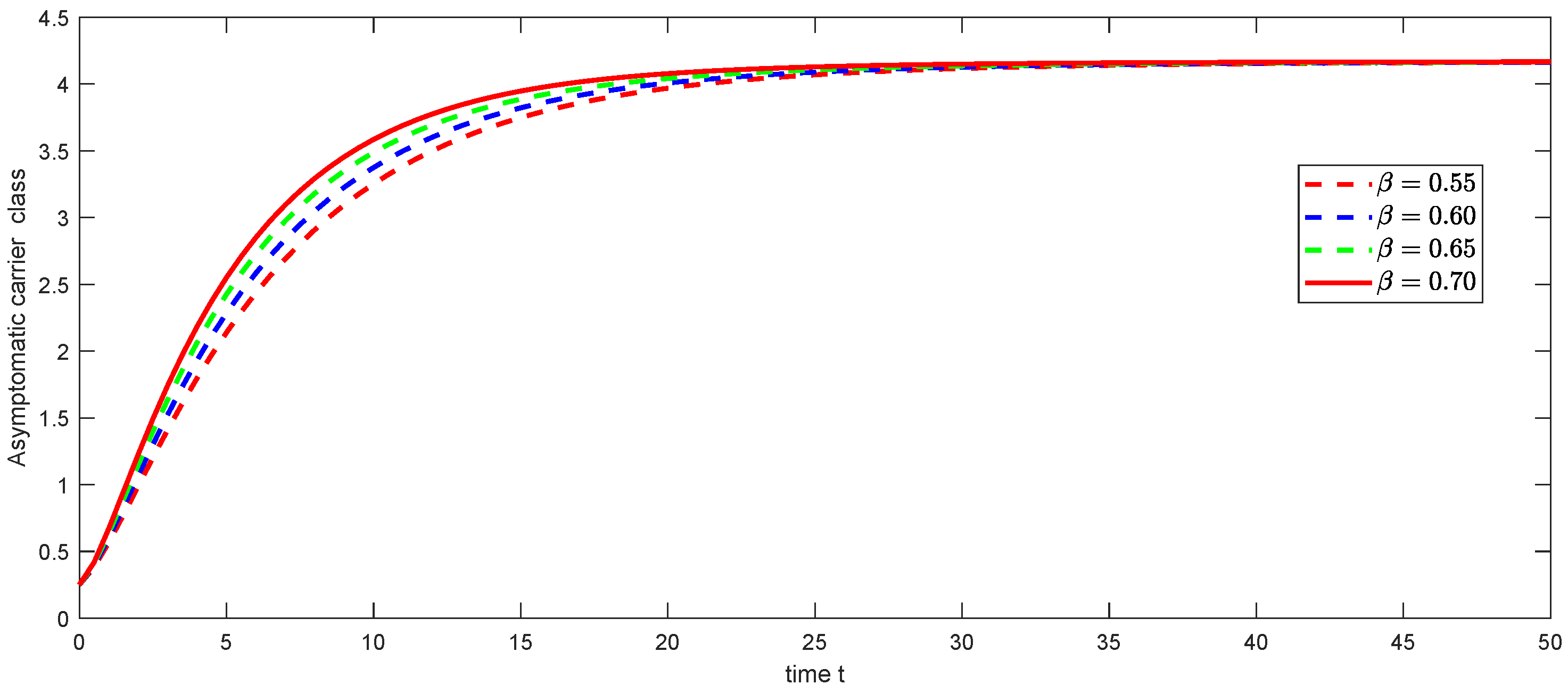
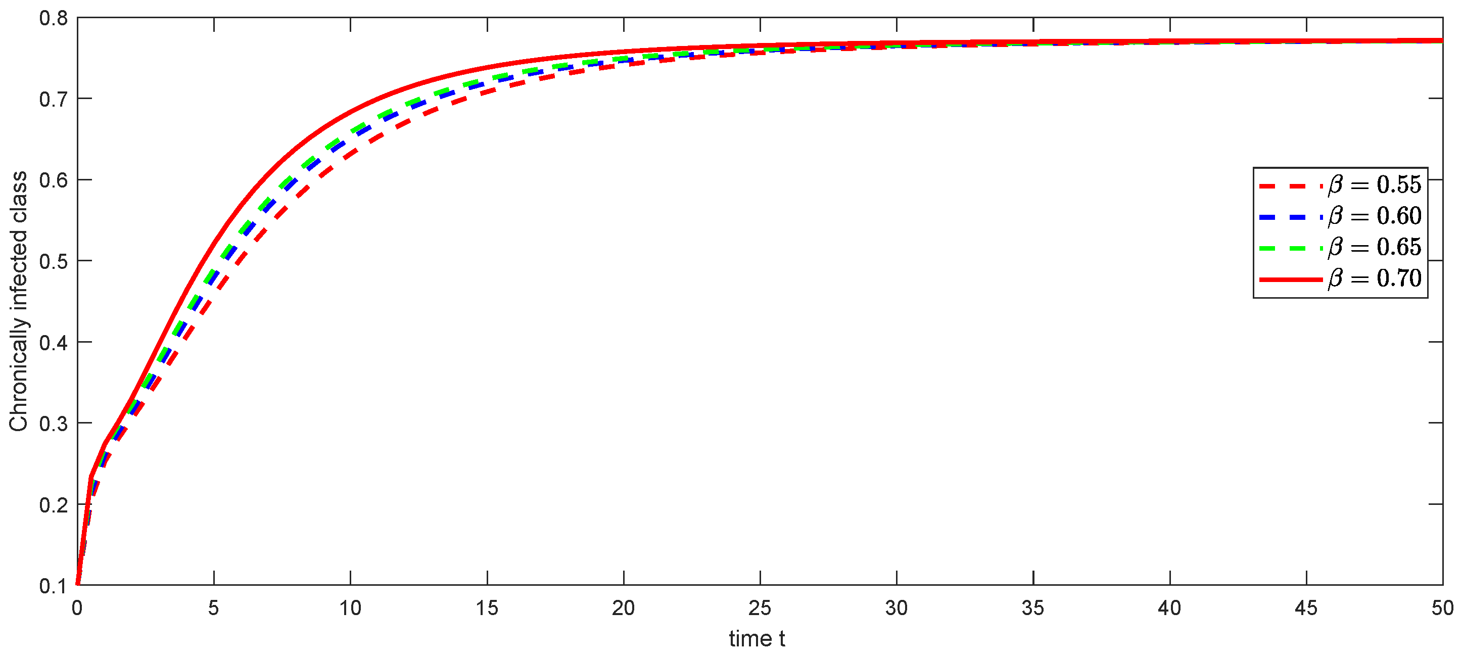
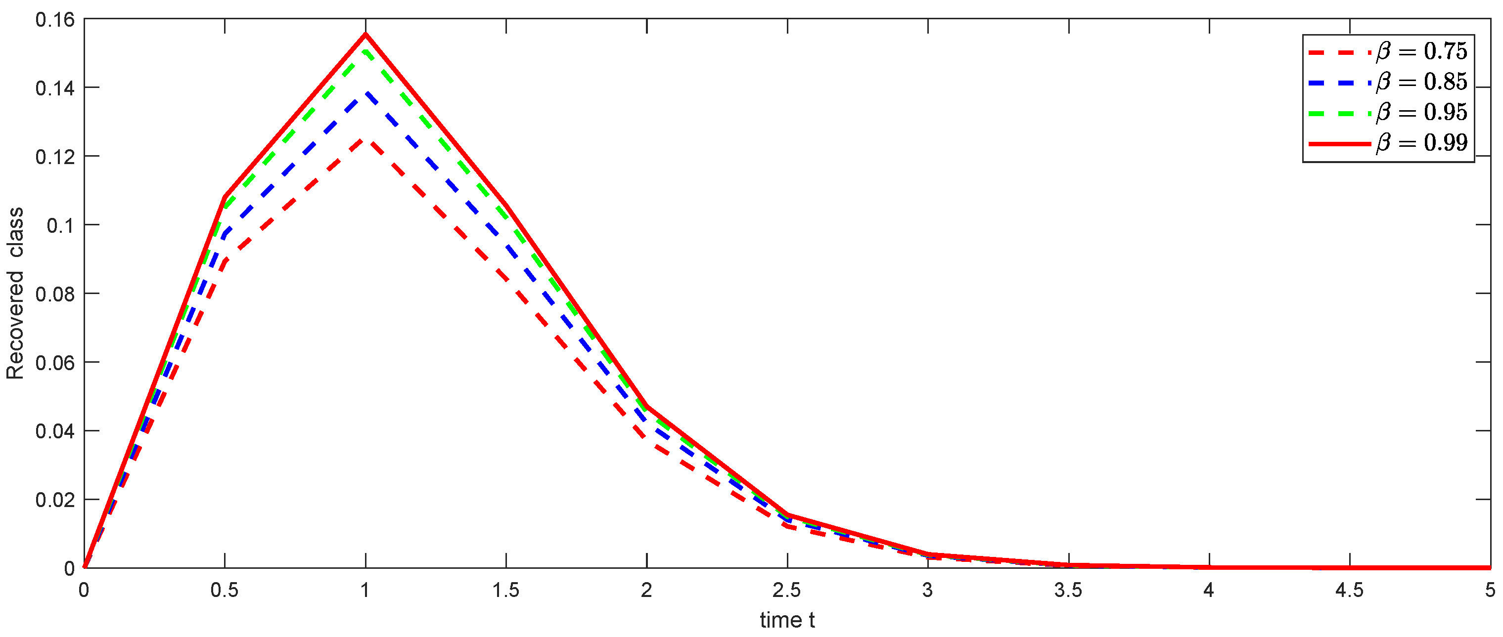
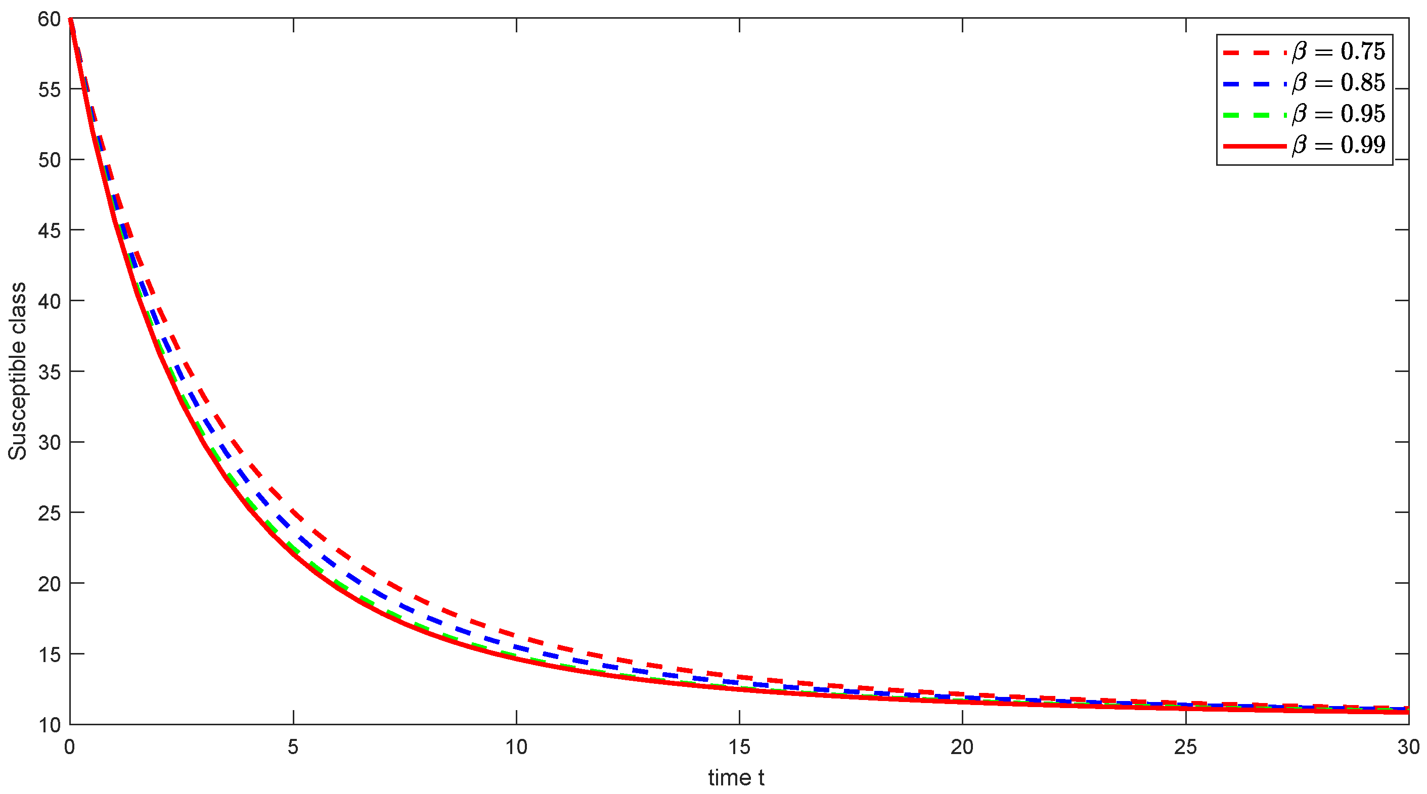
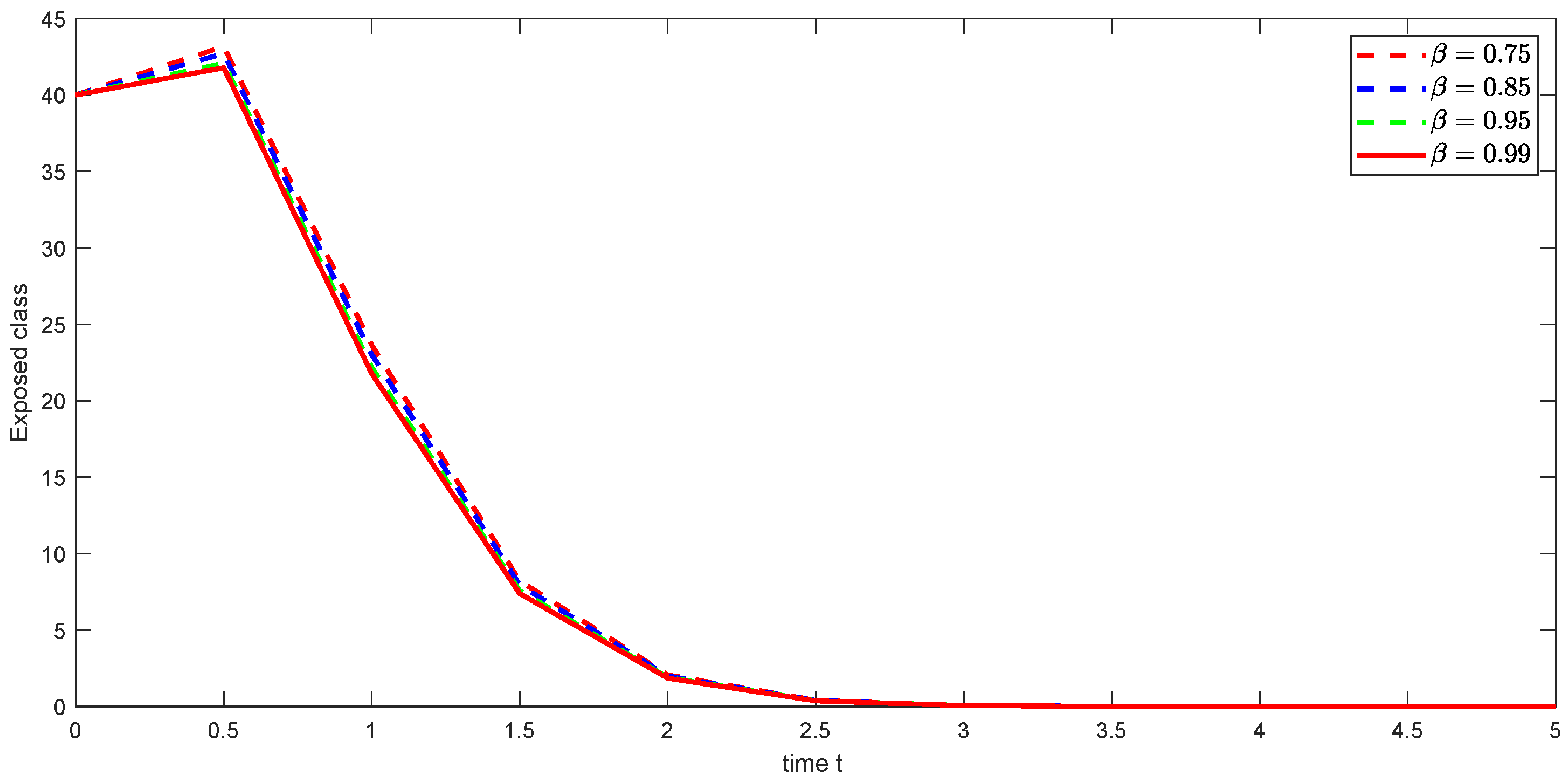
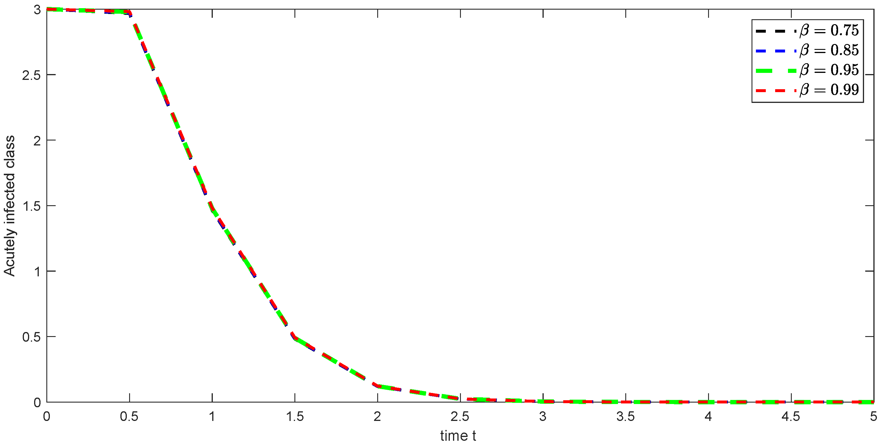
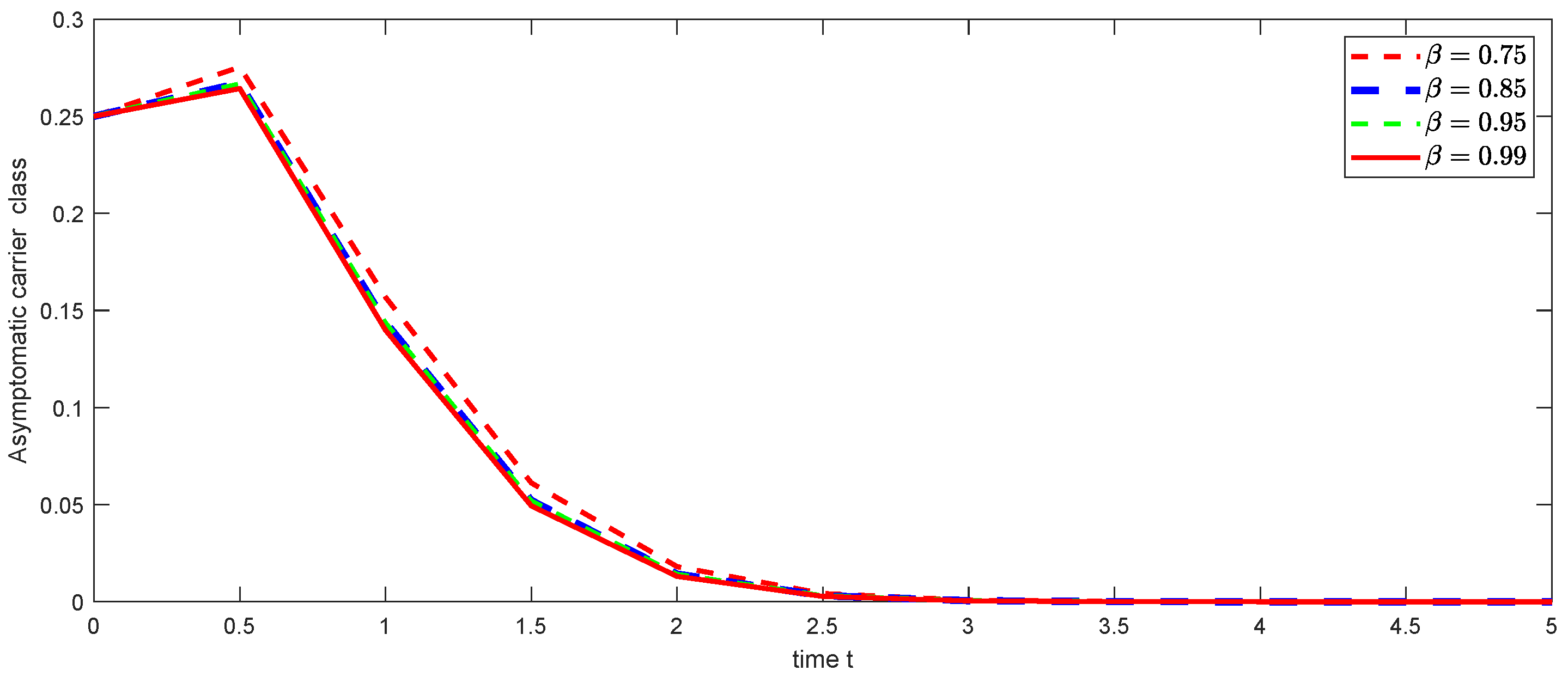
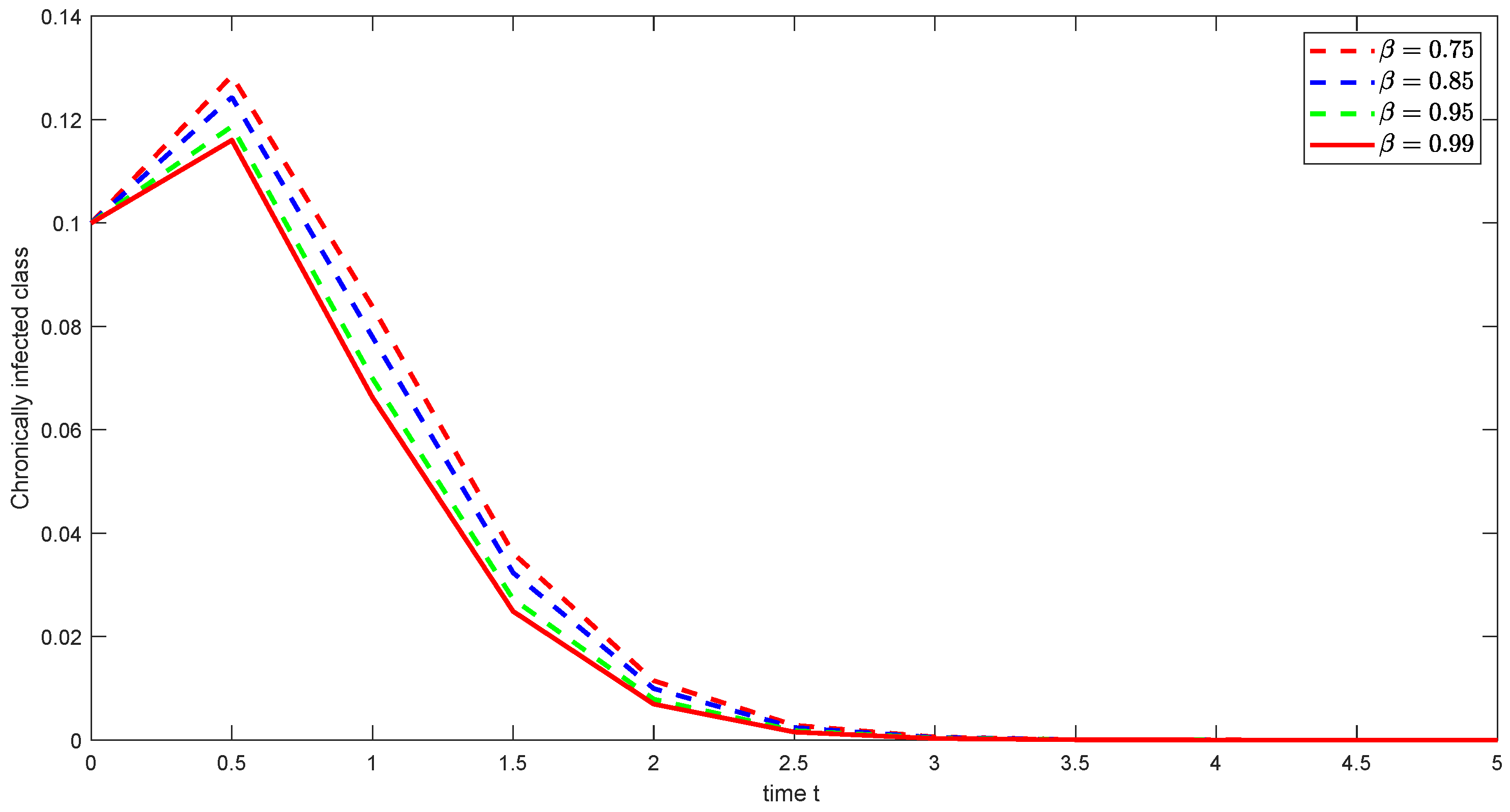
5. Application of the Numerical Scheme to an HBV Model

Controlling Hepatitis B Virus (HBV) requires a comprehensive understanding of its transmission dynamics, particularly the role of asymptomatic carriers. In this study, we extend a classical HBV model by incorporating asymptomatic carriers and analyzing its behavior using power nonlocal fractional derivatives. Our findings offer new insights that can inform improved prevention, treatment, and public health strategies.

$$\left\{\begin{array}{c}{}_{a\hspace{1em}}{}^{\mathbb{PC}}\mathbf{D}_{\varsigma ,w}^{\beta ,\delta ,p}\mathcal{S}\left(\iota \right)=\alpha -\varrho \left(\mathcal{A}+{ϵ}_1{\mathcal{A}}_c+{\omega }_1\mathcal{C}\right)\mathcal{S}-\varphi \mathcal{S},\hfill \\ {}_{a\hspace{1em}}{}^{\mathbb{PC}}\mathbf{D}_{\varsigma ,w}^{\beta ,\delta ,p}\mathcal{E}\left(\iota \right)=\varrho \left(\mathcal{A}+{ϵ}_1{\mathcal{A}}_c+{\omega }_1\mathcal{C}\right)\mathcal{S}-\left(\varphi +{\rho }_1\right)\mathcal{E},\hfill \\ {}_{a\hspace{1em}}{}^{\mathbb{PC}}\mathbf{D}_{\varsigma ,w}^{\beta ,\delta ,p}\mathcal{A}\left(\iota \right)={\rho }_1\psi \mathcal{E}-\left(\varphi +\gamma +{\mu }_1+{\kappa }_1\right)\mathcal{A},\hfill \\ {}_{a\hspace{1em}}{}^{\mathbb{PC}}\mathbf{D}_{\varsigma ,w}^{\beta ,\delta ,p}\left(\iota \right)={\rho }_1\left(1-\psi \right)\mathcal{E}-\left(\varphi +{\tau }_1+\eta \right){\mathcal{A}}_c,\hfill \\ {}_{a\hspace{1em}}{}^{\mathbb{PC}}\mathbf{D}_{\varsigma ,w}^{\beta ,\delta ,p}\mathcal{C}\left(\iota \right)={\mu }_1\mathcal{A}+{\tau }_1{\mathcal{A}}_c-\left(\varphi +\xi +{\sigma }_1\right)\mathcal{C},\hfill \\ {}_{a\hspace{1em}}{}^{\mathbb{PC}}\mathbf{D}_{\varsigma ,w}^{\beta ,\delta ,p}{\mathcal{R}}_p\left(\iota \right)={\kappa }_1\mathcal{A}+{\sigma }_1\mathcal{C}+\eta {\mathcal{A}}_c-\varphi {\mathcal{R}}_p.\hfill \end{array}\right.$$

(24)

This model tracks the dynamics of HBV across six population classes. Susceptible individuals enter the population at a birth rate of $\alpha$. The model incorporates an effective contact rate $\varrho$ and a natural fatality rate $\varphi$. Upon exposure, individuals transition to an infected state at a rate of ${\rho }_1\left(1-\psi \right)$. A fraction ${\rho }_1\psi$ of these individuals becomes acutely infected (class $\mathcal{A}$), while a portion transitions to an asymptomatic carrier state (${\mathcal{A}}_c$). Acute and asymptomatic individuals become carriers at rates ${\mu }_1$ and ${\tau }_1$, respectively. The model also includes recovery rates for acute ${\kappa }_1$, asymptomatic $\eta$, and carrier individuals ${\sigma }_1$. Disease-related death rates are denoted by $\gamma$ for acute infections and $\xi$ for chronic infections. Finally, ${ϵ}_1$ and ${\omega }_1$ represent the relative infectiousness of asymptomatic and chronic infections compared to acute infections, respectively. The total population, $\mathcal{N}\left(\iota \right)$, is categorized into susceptible ($\mathcal{S}\left(\iota \right)$), exposed ($\mathcal{E}\left(\iota \right)$), acutely infected ($\mathcal{A}\left(\iota \right)$), asymptomatic carrier (${\mathcal{A}}_c\left(\iota \right)$), chronically infected ($\mathcal{C}\left(\iota \right)$), and recovered (${\mathcal{R}}_p\left(\iota \right)$) such that $\mathcal{N}\left(\iota \right)=\mathcal{S}\left(\iota \right)+\mathcal{E}\left(\iota \right)+\mathcal{A}\left(\iota \right)+{\mathcal{A}}_c\left(\iota \right)+\mathcal{C}\left(\iota \right)+{\mathcal{R}}_p\left(\iota \right)$, with initial conditions $\mathcal{S}\left(0\right)>0,\mathcal{E}\left(0\right)>0,\mathcal{A}\left(0\right)>0,{\mathcal{A}}_c\left(0\right)>0,\mathcal{C}\left(0\right)>0$ and ${\mathcal{R}}_p\left(0\right)>0.$

We will illustrate the behavior of the power nonlocal fractional HBV transmission model (24) and its symmetric cases (Caputo–Fabrizio, Atangana–Baleanu, weighted Atangana–Baleanu, and Hattaf derivatives) using graphical representations. These graphics will show how the model’s solutions change when varying the fractional order $\beta \in \left(0,1\right)$ and other key biological parameters $\alpha =2,$$\varphi ={\displaystyle \frac{1}{67.7}},$$\varrho =0.042,$${ϵ}_1={\omega }_1=0.002,$${\rho }_1=0.004,$$\psi =0.6,$$\gamma =0.001,$${\mu }_1={\kappa }_1={\tau }_1=0.02,$$\eta =0.1,$$\xi =0.003$ and ${\sigma }_1=0.2$. In addition, the initial values are selected as ${\mathcal{S}}_0=60,{\mathcal{E}}_0=40,{\mathcal{A}}_0=3,{\mathcal{A}}_c=0.25,{\mathcal{C}}_0=0.1$ and ${\mathcal{R}}_{p0}=0.$ The numerical approximate solution of power nonlocal fractional HBV transmission model (24) with different fractional order $\beta \in \left(0,0.75\right)$ and $\delta ={\displaystyle \frac{1}{4}}$ with $p=100$, and weight function $w\left(\varsigma \right)=\varsigma$ is displayed in Figure 1, Figure 2, Figure 3, Figure 4, Figure 5 and Figure 6.

6. Symmetric Cases

Here, we present the approximate numerical solutions of four symmetric cases of the model (24) as follows:

• Case 1: The numerical approximate solution of weighted generalized Hattaf fractional HBV transmission model (24) with different fractional order $\beta \in \left(0,1\right)$ and $\delta ={\displaystyle \frac{1}{4}}$ with $p=e$, and weight function $w\left(\varsigma \right)=\varsigma$ is displayed in Figure 7, Figure 8, Figure 9, Figure 10, Figure 11 and Figure 12, respectively.
• Case 2: The numerical approximate solution of Atangana–Baleanu fractional HBV transmission model (24) with different fractional order $\beta \in (0.70,1)$ and $\delta =\beta$ with $p=e$, and weight function $w\left(\varsigma \right)=1$ is displayed in Figure 13, Figure 14, Figure 15, Figure 16, Figure 17 and Figure 18, respectively.
  [H]
• Case 3: The numerical approximate solution of weighted Atangana–Baleanu fractional HBV transmission model (24) with different fractional order $\beta \in (0.70,1)$ and $\delta =\beta$ with $p=e$, and weight function $w\left(\varsigma \right)=\varsigma$ is displayed in Figure 19, Figure 20, Figure 21, Figure 22, Figure 23 and Figure 24, respectively.
• Case 4: The numerical approximate solution of Caputo–Fabrizio fractional HBV transmission model (24) with different fractional order $\beta \in (0.70,1)$ and $\delta =1$ with $p=e$, and weight function $w\left(\varsigma \right)=1$ is displayed in Figure 25, Figure 26, Figure 27, Figure 28, Figure 29 and Figure 30, respectively.

7. Discusion and Conclusions

While the p-Laplacian operator is a powerful tool for modeling certain systems, it also introduces some complexities in analysis. In particular, the analysis is more challenging than with a typical Laplacian operator, and the results concerning the existence and uniqueness of solutions for the model are only valid under certain conditions, or when using specific values of the parameter ’p’. Despite these limitations, the inclusion of the p-Laplacian operator is essential to capture the characteristics of the complex systems considered in this study, especially in applications of non-Newtonian fluids, porous media, and image processing. It is important to point out that this added complexity is an expected tradeoff for the flexibility offered by the p-Laplacian.

Across all the symmetric cases (Hattaf, Atangana–Baleanu, weighted Atangana–Baleanu, and Caputo–Fabrizio), similar qualitative trends are observed for all classes, demonstrating the unifying property of the PFD framework. The specific choices of parameters, including the fractional order $\beta$ and the kernel structure, lead to variations in the convergence rates and steady-state values, highlighting the versatility and tunable nature of nonlocal power fractional operators. The numerical simulations effectively capture the dynamic interactions among various population classes, underscoring the relevance of this approach to real-world public health modeling. This study employs graphical representations to analyze the dynamic behavior of an HBV transmission model using PFD. The graphs illustrate the evolution of six key epidemiological classes: susceptible, exposed, acutely infected, asymptomatic carrier, chronically infected, and recovered over time. By varying the fractional order parameter $\beta$ and considering four different derivative cases (Hattaf, Atangana–Baleanu, weighted Atangana–Baleanu, and Caputo–Fabrizio), these visualizations allow for comparative analysis of the influence of memory effects on disease dynamics. The PFD framework, encompassing Hattaf, Atangana–Baleanu, weighted Atangana–Baleanu, and Caputo–Fabrizio derivatives, provides a versatile approach to modeling HBV transmission, capturing diverse memory effects inherent in biological systems. Across the six aforementioned classes, the fractional order parameter $\beta$ modulates the temporal dynamics, with lower $\beta$ values reflecting a more gradual evolution of the population classes and a heightened influence of historical data and higher $\beta$ values indicating a faster transition and the dominance of recent events. Specifically, the choice of kernel structure (exponential for Caputo–Fabrizio and Mittag–Leffler for Atangana–Baleanu) provides different mechanisms for capturing the memory effects, thus leading to distinct patterns in the evolution of different stages of HBV infection. While all four cases produce similar qualitative trends, the weighted Atangana–Baleanu and Hattaf derivatives offer increased flexibility with their additional weighting parameters, thus adapting the model based on the system dynamics. Hence, a model using a higher $\beta$ parameter should be employed for systems with faster transitions, while a model with a lower $\beta$ parameter should be used when longer-term effects and gradual transitions are of interest.

The graphical representations illustrate the effect of different fractional order parameters on the time evolution of the different epidemiological classes. In particular, the fractional order ’$\beta$’ modulates the convergence rate towards steady-states, as shown in the graphs for susceptible, exposed, infected, asymptomatic carriers and chronically infected and recovered individuals. The change in fractional orders shows significant differences in the behavior of the system, with a lower $\beta$ parameter associated with a more gradual evolution of the population classes, indicating that the past has more influence in the actual state, and a higher $\beta$ parameter associated with a faster transition, indicating that recent events dominate the dynamics. While the qualitative trend is similar for all cases, the different values of $\beta$ result in changes in the rate of convergence and the time when the steady state is achieved. This is very relevant to the modeling of real-world phenomena, allowing for a better fitting of the parameters to the system under analysis, in order to create more accurate models. These changes clearly show the tunable nature of the fractional derivatives used in this work. Future research should explore extending the proposed model to incorporate additional biological factors, such as immune response dynamics and antiviral therapy effects. Additionally, further numerical experiments could validate the theoretical results by comparing them with real-world epidemiological data.

References

1. Podlubny, I. Fractional Differential Equations; Academic Press: San Diego, CA, USA, 1999. [Google Scholar]
2. Samko, S.G.; Kilbas, A.A.; Marichev, O.I. Fractional Integrals and Derivatives; Gordon & Breach: Yverdon, Switzerland, 1993. [Google Scholar]
3. Magin, R.L. Fractional Calculus in Bioengineering. 2; Begell House: Redding, CA, USA, 2006. [Google Scholar]
4. Kilbas, A.A.; Srivastava, H.M.; Trujillo, J.J. Theory and Applications of Fractional Differential Equations. North-Holland Mathematics Studies; Elsevier: Amsterdam, The Netherlands, 2006. [Google Scholar]
5. Baleanu, D.; Diethelm, K.; Scalas, E.; Trujillo, J.J. Fractional Calculus. In Series on Complexity, Nonlinearity and Chaos; World Scientific Publishing Co. Pte. Ltd.: Hackensack, NJ, USA, 2012; Volume 3. [Google Scholar]
6. Srivastava, H.M.; Saad, K.M. Some new models of the time-fractional gas dynamics equation. Adv. Math. Models Appl. 2018, 3, 5–17. [Google Scholar]
7. Yadav, P.; Jahan, S.; Shah, K.; Peter, O.J.; Abdeljawad, T. Fractional-order modelling and analysis of diabetes mellitus: Utilizing the Atangana-Baleanu Caputo (ABC) operator. Alex. Eng. J. 2023, 81, 200–209. [Google Scholar] [CrossRef]
8. Aldwoah, K.A.; Almalahi, M.A.; Shah, K. Theoretical and numerical simulations on the hepatitis B virus model through a piecewise fractional order. Fractal Fract. 2023, 7, 844. [Google Scholar] [CrossRef]
9. Khan, H.; Alzabut, J.; Alfwzan, W.F.; Gulzar, H. Nonlinear dynamics of a piecewise modified ABC fractional-order leukemia model with symmetric numerical simulations. Symmetry 2023, 15, 1338. [Google Scholar] [CrossRef]
10. Lee, S.; Kim, H.; Jang, B. A Novel Numerical Method for Solving Nonlinear Fractional-Order Differential Equations and Its Applications. Fractal Fract. 2024, 8, 65. [Google Scholar] [CrossRef]
11. Azeem, M.; Farman, M.; Akgül, A.; De la Sen, M. Fractional order operator for symmetric analysis of cancer model on stem cells with chemotherapy. Symmetry 2023, 15, 533. [Google Scholar] [CrossRef]
12. Almalahi, M.A.; Aldowah, K.; Alqarni, F.; Hleili, M.; Shah, K.; Birkea, F.M. On modified Mittag–Leffler coupled hybrid fractional system constrained by Dhage hybrid fixed point in Banach algebra. Sci. Rep. 2024, 14, 30264. [Google Scholar] [CrossRef] [PubMed]
13. Alraqad, T.; Almalahi, M.A.; Mohammed, N.; Alahmade, A.; Aldwoah, K.A.; Saber, H. Modeling Ebola Dynamics with a Φ-Piecewise Hybrid Fractional Derivative Approach. Fractal Fract. 2024, 8, 596. [Google Scholar] [CrossRef]
14. Boutiara, A.; Abdo, M.S.; Almalahi, M.A.; Ahmad, H.; Ishan, A. Implicit hybrid fractional boundary value problem via generalized Hilfer derivative. Symmetry 2021, 13, 1937. [Google Scholar] [CrossRef]
15. Rahman, S.U.; Palencia, J.L.D. Regularity and analysis of solutions for a MHD flow with a p-Laplacian operator and a generalized Darcy-Forchheimer term. Eur. Phys. J. Plus 2022, 137, 1328. [Google Scholar] [CrossRef]
16. Alfwzan, W.F.; Khan, H.; Alzabut, J. Stability analysis for a fractional coupled Hybrid pantograph system with p-Laplacian operator. Results Control. Optim. 2024, 14, 100333. [Google Scholar] [CrossRef]
17. Boutiara, A.; Abdo, M.S.; Almalahi, M.A.; Shah, K.; Abdalla, B.; Abdeljawad, T. Study of Sturm–Liouville boundary value problems with p-Laplacian by using generalized form of fractional order derivative. AIMS Math 2022, 7, 18360–18376. [Google Scholar] [CrossRef]
18. Lotfi, E.M.; Zine, H.; Torres, D.F.M.; Yousfi, N. The power fractional calculus: First definitions and properties with applications to power fractional differential equations. Mathematics 2022, 10, 3594. [Google Scholar] [CrossRef]
19. Caputo, M.; Fabrizio, M. A new definition of fractional derivative without singular kernel. Prog. Fract. Differ. Appl. 2015, 1, 73–85. [Google Scholar]
20. Atangana, A.; Baleanu, D. New fractional derivatives with non-local and nonsingular kernel: Theory and application to heat transfer model. Therm. Sci. 2016, 20, 763–769. [Google Scholar] [CrossRef]
21. Al-Refai, M. On weighted Atangana-Baleanu fractional operators. Adv. Difference Equ. 2020, 11, 3. [Google Scholar] [CrossRef]
22. Hattaf, K. A new generalized definition of fractional derivative with non-singular kernel. Computation 2020, 8, 49. [Google Scholar] [CrossRef]
23. Zitane, H.; Torres, D.F. A class of fractional differential equations via power non-local and non-singular kernels: Existence, uniqueness and numerical approximations. Phys. D Nonlinear Phenom. 2024, 457, 133951. [Google Scholar] [CrossRef]
24. Cheng, L.; Guo, L. Positive Solution Pairs for Coupled p-Laplacian Hadamard Fractional Differential Model with Singular Source Item on Time Variable. Fractal Fract. 2024, 8, 682. [Google Scholar] [CrossRef]
25. Zhou, J.; Gong, C.; Wang, W. The Sign-Changing Solution for Fractional (p, q)-Laplacian Problems Involving Supercritical Exponent. Fractal Fract. 2024, 8, 186. [Google Scholar] [CrossRef]
26. Rahman, S.U.; Díaz Palencia, J.L. Analytical and Computational Approaches for Bi-Stable Reaction and p-Laplacian Diffusion Flame Dynamics in Porous Media. Mathematics 2024, 12, 216. [Google Scholar] [CrossRef]
27. Yang, D.; Bai, Z.; Bai, C. Existence of Solutions for Nonlinear Choquard Equations with (p, q)-Laplacian on Finite Weighted Lattice Graphs. Axioms 2024, 13, 762. [Google Scholar] [CrossRef]
28. Al-Refai, M.; Jarrah, A.M. Fundamental results on weighted Caputo–Fabrizio fractional derivative. Chaos Solitons Fractals 2019, 126, 7–11. [Google Scholar] [CrossRef]
29. Hattaf, K. On some properties of the new generalized fractional derivative with non-singular kernel. Math. Probl. Eng. 2021, 1, 1580396. [Google Scholar] [CrossRef]
30. Khan, H.; Chen, W.; Sun, H.G. Analysis of positive solution and Hyers-Ulam stability for a class of singular fractional differential equations with p-Laplacian in Banach space. Math. Meth. Appl. Sci. 2018, 41, 3430–3440. [Google Scholar] [CrossRef]
31. Khan, H.; Li, Y.; Suna, H.; Khan, A. Existence of solution and Hyers-Ulam stability for a coupled system of fractional differential equations with p-Laplacian operator. Bound. Value Probl. 2017, 2017, 157. [Google Scholar] [CrossRef]
32. Ibrahim, R.W. Generalized Hyers-Ulam stability for fractional differential equations. Int. J. Math. 2012, 23, 1250056. [Google Scholar] [CrossRef]
Figure 1. Graphical illustration of approximate solution for susceptible class using different values of β ( 0 , 0.75 ) , and δ = 1 4 with power p = 100 .
Fractalfract 09 00092 g001
Figure 2. Graphical illustration of approximate solution for exposed class using different values of β ( 0 , 0.75 ) , and δ = 1 4 with power p = 100 .
Fractalfract 09 00092 g002
Figure 3. Graphical illustration of approximate solution for acutely infected class using different values of β ( 0 , 0.75 ) , and δ = 1 4 with power p = 100 .
Fractalfract 09 00092 g003
Figure 4. Graphical illustration of approximate solution for asymptomatic carrier class using different values of β ( 0 , 0.75 ) , and δ = 1 4 with power p = 100 .
Fractalfract 09 00092 g004
Figure 5. Graphical illustration of approximate solution for chronically class using different values of β ( 0 , 0.75 ) , and δ = 1 4 with power p = 100 .
Fractalfract 09 00092 g005
Figure 6. Graphical illustration of approximate solution for recovered class using different values of β ( 0 , 0.75 ) , and δ = 1 4 with power p = 100 .
Fractalfract 09 00092 g006
Figure 7. Graphical illustration of approximate solution for susceptible class using different values of β ( 0.70 , 1 ) , and δ = 1 4 with power p = e .
Fractalfract 09 00092 g007
Figure 8. Graphical illustration of approximate solution for exposed class using different values of β ( 0.70 , 1 ) , and δ = 1 4 with power p = e .
Fractalfract 09 00092 g008
Figure 9. Graphical illustration of approximate solution for acutely infected class using different values of β ( 0.70 , 1 ) , and δ = 1 4 with power p = e .
Fractalfract 09 00092 g009
Figure 10. Graphical illustration of approximate solution for asymptomatic carrier class using different values of β ( 0.70 , 1 ) , and δ = 1 4 with power p = e .
Fractalfract 09 00092 g010
Figure 11. Graphical illustration of approximate solution for chronically class using different values of β ( 0.70 , 1 ) , and δ = 1 4 with power p = e .
Fractalfract 09 00092 g011
Figure 12. Graphical illustration of approximate solution for recovered class using different values of β ( 0.70 , 1 ) , and δ = 1 4 with power p = e .
Fractalfract 09 00092 g012
Figure 13. Graphical illustration of approximate solution for susceptible class using different values of δ = β ( 0.70 , 1 ) with power p = e .
Fractalfract 09 00092 g013
Figure 14. Graphical illustration of approximate solution for exposed class using different values of δ = β ( 0.70 , 1 ) with power p = e .
Fractalfract 09 00092 g014
Figure 15. Graphical illustration of approximate solution for acutely infected class using different values of δ = β ( 0.70 , 1 ) with power p = e .
Fractalfract 09 00092 g015
Figure 16. Graphical illustration of approximate solution for asymptomatic carrier class using different values of δ = β ( 0.70 , 1 ) with power p = e .
Fractalfract 09 00092 g016
Figure 17. Graphical illustration of approximate solution for chronically class using different values of δ = β ( 0.70 , 1 ) with power p = e .
Fractalfract 09 00092 g017
Figure 18. Graphical illustration of approximate solution for recovered class using different values of δ = β ( 0.70 , 1 ) with power p = e .
Fractalfract 09 00092 g018
Figure 19. Graphical illustration of approximate solution for susceptible class using different values of δ = β ( 0.70 , 1 ) with power p = e .
Fractalfract 09 00092 g019
Figure 20. Graphical illustration of approximate solution for exposed class using different values of δ = β ( 0.70 , 1 ) with power p = e .
Fractalfract 09 00092 g020
Figure 21. Graphical illustration of approximate solution for acutely infected class using different values of δ = β ( 0.70 , 1 ) with power p = e .
Fractalfract 09 00092 g021
Figure 22. Graphical illustration of approximate solution for asymptomatic carrier class using different values of δ = β ( 0.70 , 1 ) with power p = e .
Fractalfract 09 00092 g022
Figure 23. Graphical illustration of approximate solution for chronically class using different values of δ = β ( 0.70 , 1 ) with power p = e .
Fractalfract 09 00092 g023
Figure 24. Graphical illustration of approximate solution for recovered class using different values of δ = β ( 0.70 , 1 ) with power p = e .
Fractalfract 09 00092 g024
Figure 25. Graphical illustration of approximate solution for susceptible class using different values of δ = 1 , β ( 0.70 , 1 ) with power p = e .
Fractalfract 09 00092 g025
Figure 26. Graphical illustration of approximate solution for exposed class using different values of δ = 1 , β ( 0.70 , 1 ) with power p = e .
Fractalfract 09 00092 g026
Figure 27. Graphical illustration of approximate solution for acutely infected class using different values of δ = 1 , β ( 0.70 , 1 ) with power p = e .
Fractalfract 09 00092 g027
Figure 28. Graphical illustration of approximate solution for asymptomatic carrier class using different values of δ = 1 , β ( 0.70 , 1 ) with power p = e .
Fractalfract 09 00092 g028
Figure 29. Graphical illustration of approximate solution for chronically class using different values of δ = 1 , β ( 0.70 , 1 ) with power p = e .
Fractalfract 09 00092 g029
Figure 30. Graphical illustration of approximate solution for recovered class using different values of δ = 1 , β ( 0.70 , 1 ) with power p = e .
Fractalfract 09 00092 g030
Disclaimer/Publisher’s Note: The statements, opinions and data contained in all publications are solely those of the individual author(s) and contributor(s) and not of MDPI and/or the editor(s). MDPI and/or the editor(s) disclaim responsibility for any injury to people or property resulting from any ideas, methods, instructions or products referred to in the content.