Physics-Informed Fractional-Order Recurrent Neural Network for Fast Battery Degradation with Vehicle Charging Snippets

Abstract

To handle and manage battery degradation in electric vehicles (EVs), various capacity estimation methods have been proposed and can mainly be divided into traditional modeling methods and data-driven methods. For realistic conditions, data-driven methods take the advantage of simple application. However, state-of-the-art machine learning (ML) algorithms are still kinds of black-box models; thus, the algorithms do not have a strong ability to describe the inner reactions or degradation information of batteries. Due to a lack of interpretability, machine learning may not learn the degradation principle correctly and may need to depend on big data quality. In this paper, we propose a physics-informed recurrent neural network (PIRNN) with a fractional-order gradient for fast battery degradation estimation in running EVs to provide a physics-informed neural network that can make algorithms learn battery degradation mechanisms. Incremental capacity analysis (ICA) was conducted to extract aging characteristics, which could be selected as the inputs of the algorithm. The fractional-order gradient descent (FOGD) method was also applied to improve the training convergence and embedding of battery information during backpropagation; then, the recurrent neural network was selected as the main body of the algorithm. A battery dataset with fast degradation from ten EVs with a total of 5697 charging snippets were constructed to validate the performance of the proposed algorithm. Experimental results show that the proposed PIRNN with ICA and the FOGD method could control the relative error within $5\%$ for most snippets of the ten EVs. The algorithm could even achieve a stable estimation accuracy (relative error < 3%) during three-quarters of a battery’s lifetime, while for a battery with dramatic degradation, it was difficult to maintain such high accuracy during the whole battery lifetime.

1. Introduction

As the most commonly used energy supply for electric vehicles (EVs), the durability of lithium–ion batteries (LIBs) is a key concern for the intelligent management of batteries [1,2]. Batteries degrade according to dynamic operation conditions and environmental conditions during their lifetime; thus, capacity estimation methods for LIBs have been widely designed recently [3,4]. Currently, researchers have proposed kinds of methods for the estimation of the state of charge (SOC) [5], state of health (SOH) [6,7], and remaining useful life (RUL) [8] by various model-based methods and data-driven methods [9,10,11]. Data–driven methods include statistical methods such as entropy, correlation, and wavelet transform [12,13] and kinds of machine learning (ML) methods such as regression models, neural networks(NNs), reinforcement learning, and even transfer learning [14,15,16]. Machine learning (ML) is gradually applied to battery capacity estimation and degradation prediction in an intelligent way to make an algorithm learn the battery degradation path [17]. Among ML algorithms, NNs are a widely investigated and easily employed type for estimating the battery capacity of EVs [18], such as recurrent neural networks (RNNs), long short-term memory (LSTM) [7], and gated recurrent units (GRUs) [19]. Recently, researchers have proposed several innovative ML methods for EVs and hybrid electric vehicles (HEVs), such as optimal energy management strategies [20], supervised ML for battery health performance [21], deep learning for seasonal EV forecasting models [22], and so on.

For the convergence of the loss function and weight updates of NNs, the first-order optimal method (series of gradient descent) and second-order optimal method (series of the Hessian matrix) are developed during backpropagation processes. The calculation of the Hessian matrix may use heavy computing resources and storage; thus, its application is limited or replaced by the quasi-Newton method [23,24]. The series of gradient descent (GD) method is currently the main used optimal method, and the basic GD method is improved in several well-known GD methods, such as stochastic gradient descent (SGD), mini batch gradient descent, GD with momentum, the Nesterov accelerated gradient (NAG), adaptive gradient (Adagrad), adaptive moment estimation (Adam), and so on [25,26]. Moreover, researchers have proposed more innovative gradient-based methods, such as smoothed functional algorithms with a norm-limited update vector [27], grafting gradient descent [28], normalized simultaneous perturbation stochastic approximation (SPSA) [29], the Gaussian–Stein variational gradient descent [30], and so on. While research on GD is a thriving direction and includes a large number of methods, this paper focuses on the fractional-order information of batteries combined with GD methods; thus, the basic GD method is selected in this study.

With careful preprocessing and excellent calculation support, ML algorithms can achieve perfect performance in capacity estimation accuracy at the lab level. However, in realistic situations, these kinds of algorithms cannot develop their advantages due to limited data quality [31]. With unstable and dynamic operation conditions, battery degradation may vary from that at the lab level and cannot be predicted by pre-trained algorithms at the lab level [18]. Hence, it is necessary to make ML learn to learn battery mechanisms. In this way, an algorithm can understand the inner reactions during battery degradation from the aspect of first principles. In the previous literature, physics-informed machine learning (PIML) has been proposed to solve problems related to objects with physical laws [32]. PIML can encode a physical law of a predicted object into observational bias, inductive bias, and learning bias [32,33,34]; thus, it combines the advantages of model-based models and data-driven algorithms [35]. Informed by battery knowledge from batteries’ physical laws, the neural network can be enhanced from different aspects, such as the state’s feedback, the loss function, and the gradient in backpropagation, for application to LIBs [36,37,38]. Hence, battery information needs to find a way to be embedded into algorithms, and fractional calculus needs to come out. Fractional calculus (FC) was firstly applied to LIBs to enhance nonlinear fractional-order (FO) modeling [39,40,41,42]. The reflection of the diffusion dynamics of battery modeling was described by introducing a fractional-order element called the Warburg element [43,44]. Then, fractional-order methods, such as the FO extended Kalman filter (EKF) [45] and FO unscented Kalman filter (UKF) [46], were proposed for the estimation of battery states. Moreover, to process time–series data and their characteristics, the fractional-order recurrent neural network (FORNN), fractional-order state feedback, and the fractional-order gradient have also been investigated theoretically [37,47,48]. Since the fractional-order gradient can introduce history gradient data to improve the local optimum problem, the basic GD method was upgraded to the fractional-order gradient descent (FOGD) method, which can be applied to RNNs to express battery degradation information in time series.

In this paper, a physics-informed method is proposed to enhance algorithm interpretability. Incremental capacity analysis (ICA) is also conducted to extract degradation characteristics as the inputs for machine learning. Then, since the fractional-order element (constant phase element, CPE) can reflect the charge transfer reaction in the mid-frequency and solid diffusion dynamics in the low frequency of LIBs [43,44], a fractional-order gradient descent (FOGD) method is added to improve the convergence of the algorithm during training. To process the time–series battery data, the main body of the algorithm is chosen to be an RNN. It should be noted that the main body of the algorithm proposed in this paper is not limited to an RNN, and other suitable ML algorithms can be applied, such as LSTM, GRUs, or even meta-learning. Similarly, the FOGD method proposed in this paper can be extended to other kinds of GD methods, such as SGD, GD with momentum, and so on.

Here are the several main contributions of this paper.

• A physics-informed recurrent neural network (PIRNN) with ICA and FOGD methods is proposed for capacity estimation in LIBs with fast degradation. The peak magnitudes of the IC curves are extracted as input characteristics for the neural network, and a fractional-order gradient is applied to the backpropagation process.
• The proposed PIRNN can learn the battery information of running EVs during training convergence and achieve stable capacity estimation accuracy (relative error < 3%) using a LiFeP${\mathrm{O}}_4$ battery dataset over three-quarters of a lifetime. This demonstrates that the proposed PIRNN can be applied to realistic batteries from running EVs and hold its accuracy.
• A battery dataset with fast degradation is constructed based on ten running EVs covering the years 2018–2022 and with over a 40,000 km mileage. The dataset contains 5697 charging snippets and covers almost the whole battery lifetime, which can be the validation dataset for kinds of machine learning algorithms.

2. Preliminary

2.1. Fractional-Order Calculus and Derivative

This paper applies a fractional-order derivative in Caputo’s definition [41] to construct a fractional-order gradient descent method, and the Caputo definition can be presented as

$${}_{ }{}^{C}D_t^{\alpha }f\left(t\right)={\displaystyle \frac{1}{\mathrm{\Gamma }(n-\alpha )}}\underset{t_0}{\overset{t}{\int }}{\displaystyle \frac{f^{\left(n\right)}\left(\tau \right)}{{(t-\tau )}^{\alpha -n+1}}}\mathrm{d}\tau ,t>t_0$$

(1)

where ${}_{ }{}^{C}D_t^{\alpha }$ represents the fractional operator in the Caputo definition, $\alpha \in (n-1,n)$, and $\mathrm{\Gamma }(·)$ is the gamma function.

If $f\left(x\right)$ is smooth with a finite fractional-order derivative, the Caputo derivative in Equation (1) can be discretized as

$${}_{x_0}{}^{C}D_x^{\alpha }f\left(x\right)=\sum _{i=n}^{\infty }{\displaystyle \frac{f^{\left(i\right)}\left(x_0\right)}{\mathrm{\Gamma }(i+1-\alpha )}}{(x-x_0)}^{i-\alpha }$$

(2)

In (2), if $f\left(x\right)={(x-x_0)}^{\lambda }$, (2) can be deduced as follows [49]:

$${}_{x_0}{}^{C}D_x^{\alpha }{(x-x_0)}^{\lambda }={\displaystyle \frac{\mathrm{\Gamma }(\lambda +1)}{\mathrm{\Gamma }(\lambda -\alpha +1)}}{(x-x_0)}^{\lambda -\alpha },$$

(3)

where $\lambda -\alpha +1>0$.

Equation (2) is a discrete form and Equation (3) is a simple form for a quadratic function. We employ the Caputo derivative for the backpropagation of the neural network to calculate the fractional-order gradient in this paper.

2.2. Fractional-Order Gradient

The integer–order gradient of a smooth convex function, $f\left(x\right)$, is usually presented as $\nabla f\left(x\right)$, which is the iteration direction for the optimal point search. The discretized form of the gradient method can be presented as

$$x_{k+1}=x_k-\rho \nabla f\left(x_k\right),$$

(4)

where k is the iteration step and $x_k$ is the discrete value in step k.

The factional-order derivative introduces a fractional order, $\alpha$, to Equation (4) for complex systems and nonlinear characteristics. With the Caputo definition, the fractional-order gradient can be presented as

$$x_{k+1}=x_k-\rho {\nabla }_{x_{k-1}}^{\mathrm{C}}{D}_{x_k}^{\alpha }f\left(x\right),$$

(5)

where $0<\alpha <1$. The convergence of the fractional-order gradient in (5) depends on the fractional order $\alpha$ and initial value $x_0$. If the Caputo definition is calculated by the discrete Equation (2), (5) can converge to the global extreme point $x^{*}$. In this paper, fractional-order gradients are applied to the gradient descent method for the backpropagation of the neural network. Hence, the fractional-order characteristics of LIBs are analyzed and encoded into the network design with batteries’ physical information.

3. Battery Dataset and Its Fractional-Order Information

3.1. EV Dataset and Battery Degradation

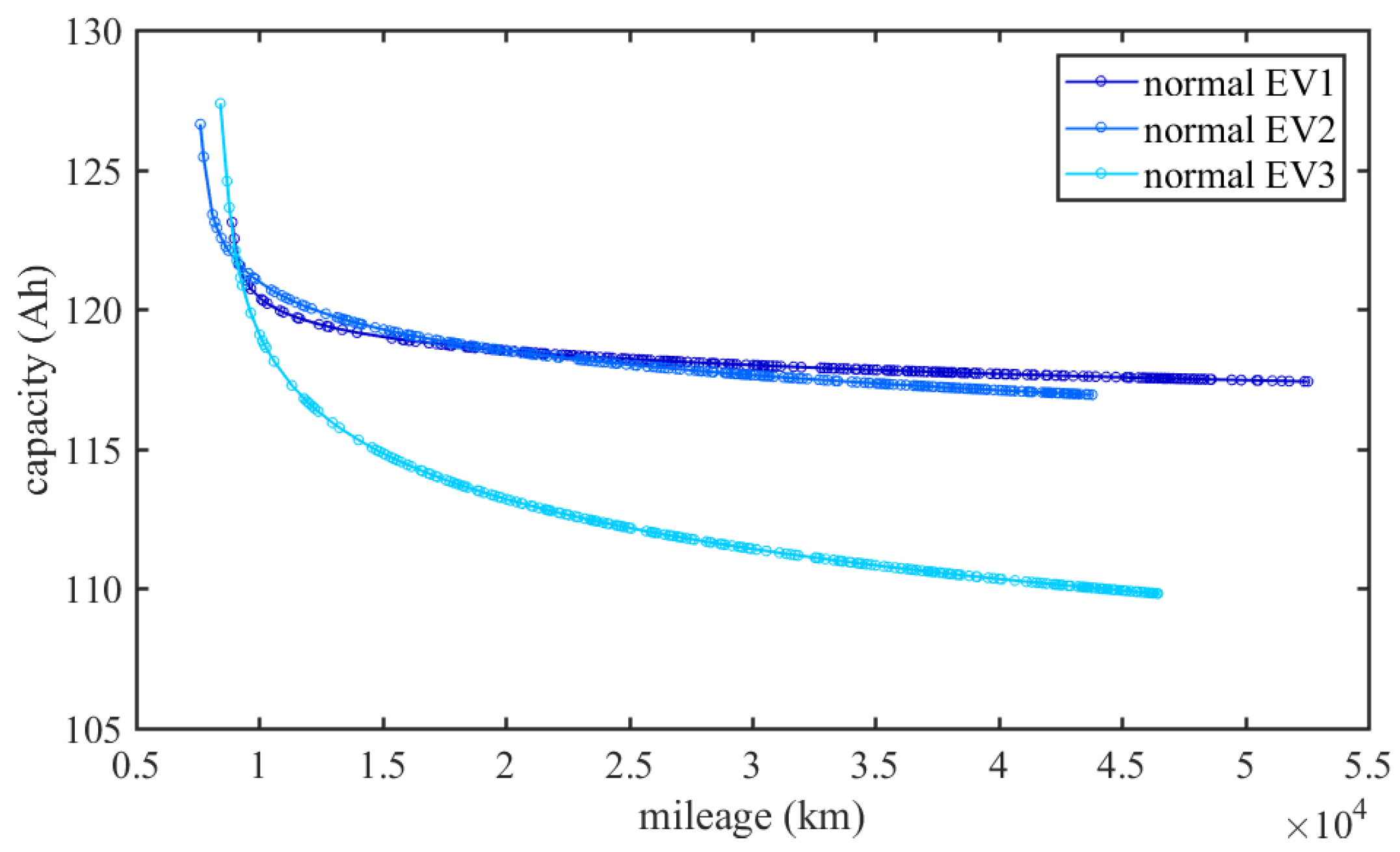
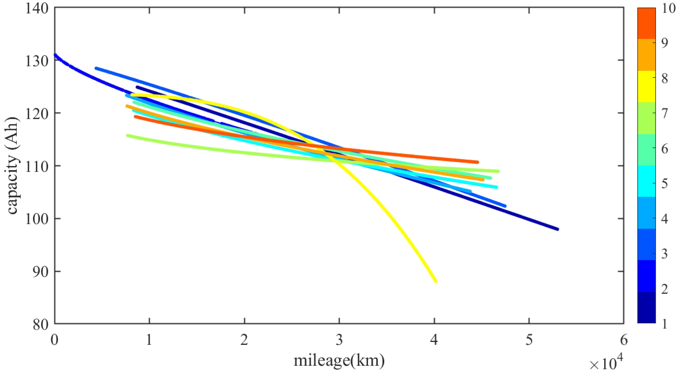
3.1.1. Battery Capacity

For battery durability, state estimations are quite important, such as the state of charge (SOC), which can be obtained by a look-up table with open circuit voltage (OCV), and state of health (SOH), which illustrates the real-time battery charging/discharging ability. The battery capacity is the basis of the SOH. For realistic data, battery capacity can be calculated as

$$Q_{\alpha ,\beta }={\displaystyle \frac{\Delta Ah}{\Delta SOC}}={\displaystyle \frac{{\int }_{t_{\alpha }}^{t_{\beta }}I\left(\tau \right)d\tau }{SOC\left(t_{\beta }\right)-SOC\left(t_{\alpha }\right)}}$$

(6)

where $t_{\alpha }$ and $t_{\beta }$ are two separate moments and $I\left(t\right)$ is the current during $(t_{\alpha },t_{\beta })$. Equation (6) is based on the Ampere-hour integral method and depth of charge (DOC). The DOC is the SOC change range during charging. The labels used in this paper are deduced and based on Equation (6) with the calibration of the SOC-OCV curve.

In general, Ni-CO-Mn (NCM) batteries and LiFeP${\mathrm{O}}_4$ (LFP) batteries are the two major kinds of LIBs used. The available battery in this paper is an LFP battery. A typical degradation fitting curve of an LFP battery under regular cycles is usually a power-law function, as shown in Figure 1. It shows a slowed-down degradation when the battery goes into the late period of its lifetime. However, under the dynamic operation conditions in EVs, the data obtained in this paper are for a set of batteries with faster degradation rather than a slow power function.

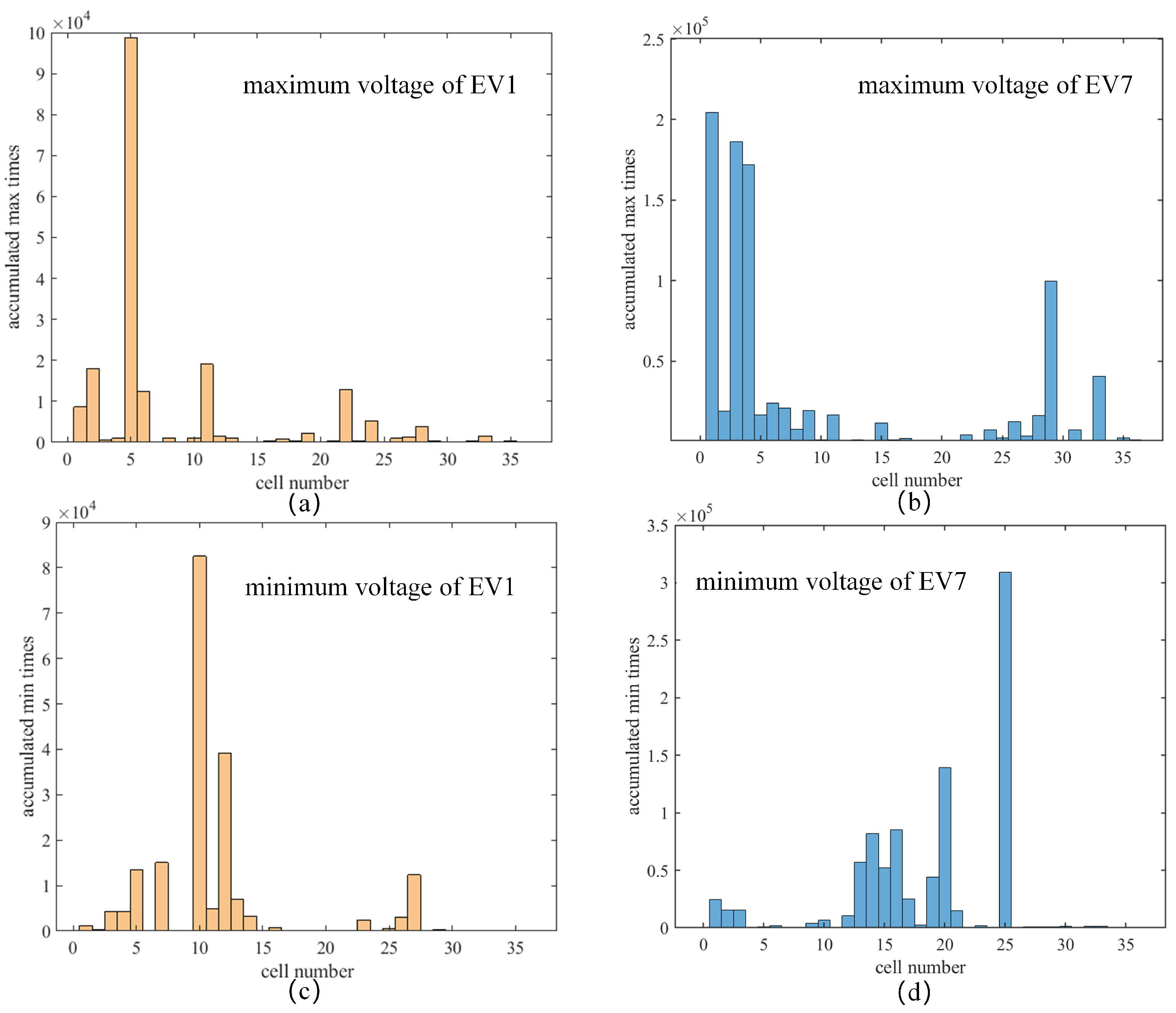
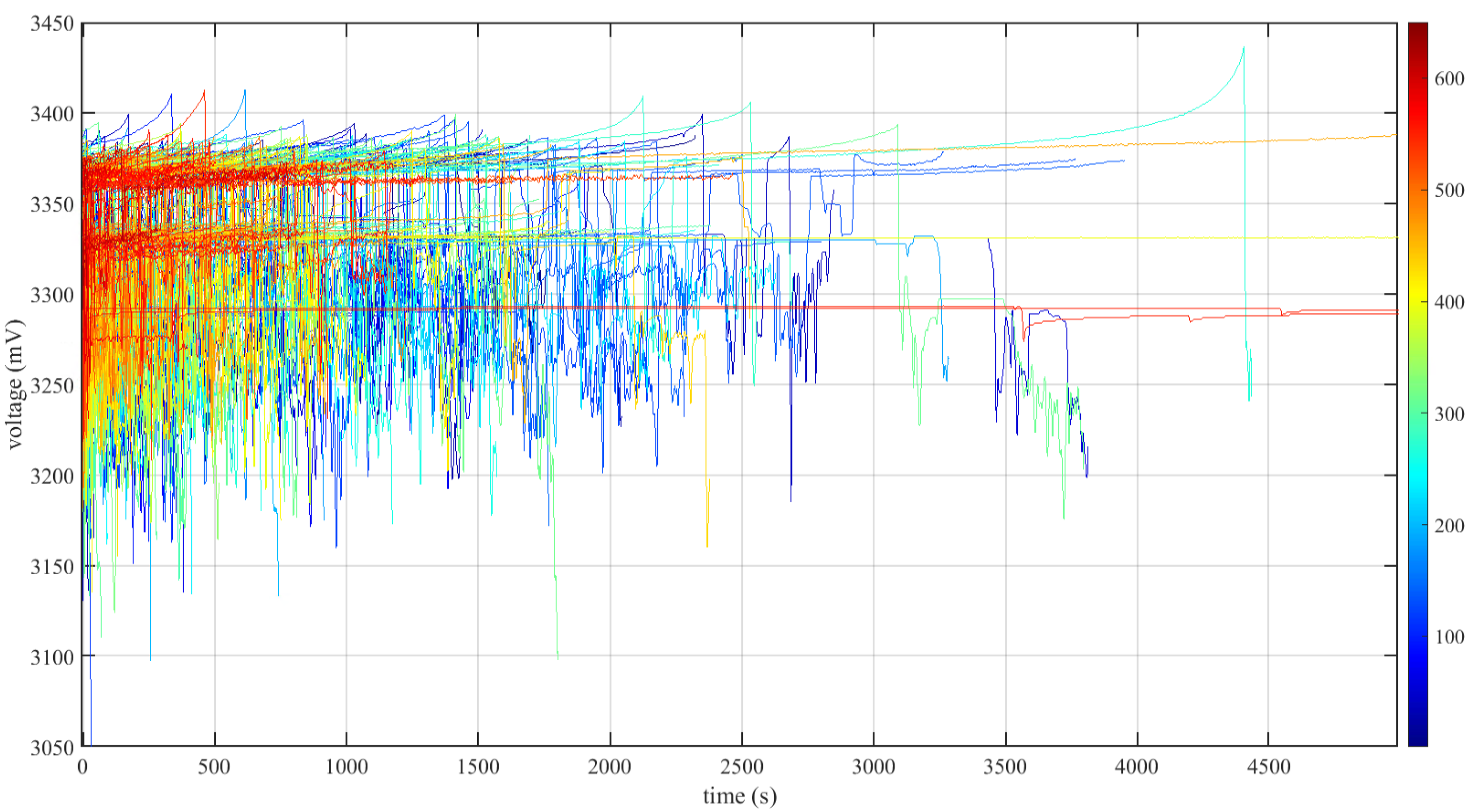
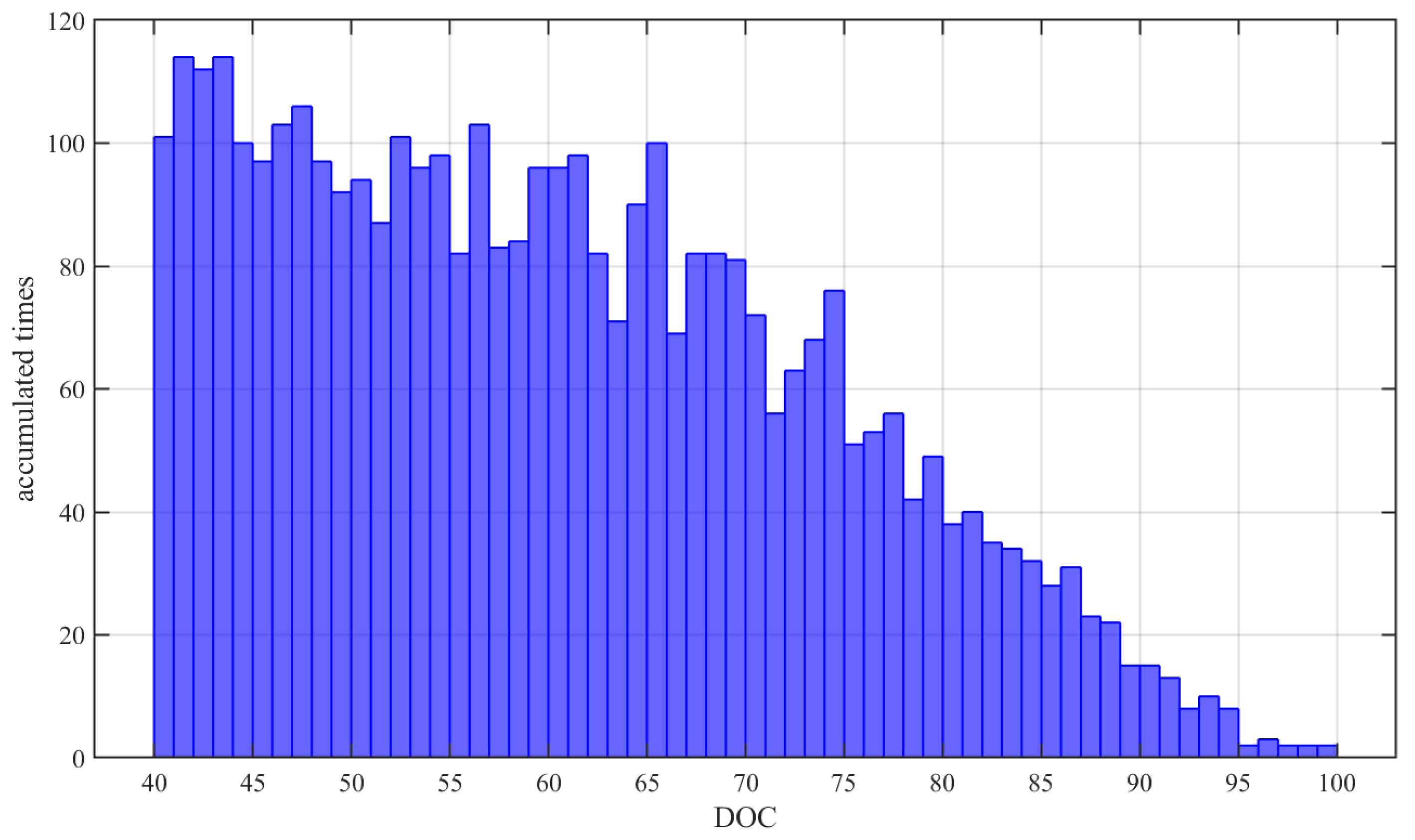
3.1.2. Battery Dataset with Vehicle Charging Snippets

The dataset used in this paper comes from our co-operation project, which contains 10 EVs named from “EV1” to “EV10” due to VIN privacy protection. Ten EVs numbered from 1 to 10 were sampled with the operation data of their power battery; then, the battery capacity was calculated, based on Equation (6) with the calibration of the SOC-OCV curve. The basic information of the ten EVs (EV1-EV10) is listed in

Table 1. Battery datatset extracted from charging snippets of ten vehicles.

EV No.	Snippets Amount	Time Range	Mileage Range (km)	SOH Range (Ah)
EV1	698	18 September 2018–28 Febraury 2022	8730–52,992	124.9076–97.9608
EV2	290	11 October 2018–29 March 2022	87–21,987	131.0177–115.6695
EV3	660	22 September 2018–28 Febraury 2022	4400–47,461	128.4828–102.3552
EV7	571	10 December 2018–31 January 2022	7605–43,792	123.3471–105.1326
EV5	633	19 September 2018–16 September 2021	8355–46,569	120.4993–105.9154
EV6	562	18 September 2018-2 March 2022	8395–45,933	122.0545–107.6695
EV7	650	18 September 2018–1 March 2022	7725–46,737	115.7236–108.9408
EV8	487	18 September 2018–31 January 2022	8165–40,186	123.4687–88.0738
EV9	590	18 September 2018–20 July 2021	7660–45,148	121.3203–107.3435
EV10	556	18 September 2018–20 December 2021	8538–44,569	119.3115–110.6705

. The battery cell used in the ten EVs is a kind of LFP cell with a 130 Ah rated capacity and 14.9 kWh rated power, and the rated voltage range is from 2.5 V to 3.65 V. The battery pack of the EV contains 36 cells connected in series. Due to the privacy protection, we could only obtain the basic rated parameter and OCV-SOC map of this LFP cell provided by our co-operation company. The driving cycles of the ten EVs are mostly urban operating conditions with various drivers instead of experimentally designed conditions. Since dynamic operation conditions result in fluctuant vehicle data, charging snippets from the EVs were selected, and data preprocessing was conducted to filter stable data to construct the battery dataset used in this paper. From Table 1, we see that the time range of the filtered battery dataset covers from 2018 to 2022 and the vehicle mileage varies from 87 to 52,992 km, which contain a long enough period and enough mileage for representing an aging LFP battery. The charging snippets were filtered by the SOC upper limit (>80%) and lower limit (<40%) so that the depth of charge (DOC) could be larger than 40%; then, the battery degradation characteristics could be deduced from the voltage curves. Although a tough filter condition was applied, the obtained snippets were enough to construct a battery dataset for degradation.

We could not obtain all the accurate capacity labels from standard capacity test, since these realistic running vehicles are possessed by customers. Hence, based on Equation (6), Figure 2 shows the calculated capacities used as labels in this paper, and the rated capacity of this battery pack in these ten EVs is 130 Ah. Compared to Figure 1, the battery degradation shown in Figure 2 presents faster trends during the battery lifetime. Based on the obtained data, this may be caused by the chemical composition of this type of LFP battery or caused by the dynamic operation conditions. The fast degradation mentioned in this paper produces the aging curves shown in Figure 2, which are different from the general power-law trend. It should be noted that we do not discuss the specific capacity plunge (dramatic capacity decrease) in this paper, although it can be observed that EV8 in Figure 2 holds an abnormal aging curve with an almost 30% degradation. The battery capacity plunge is another worthy investigation topic in our other works, and our work in this paper is the employment of the PIRNN with a physics-informed method with this dataset containing ten EVs.

3.2. Fractional-Order Information of Battery

3.2.1. Fractional-Order Equivalent Circuit Model

An electrochemical model with partial differential equations (PDEs) can describe the physical laws of LIBs at the microscopic particle level, such as lithium ion concentrations, potential distributions, and interface Bulter–Volmer kinetics; however, the particle-level reactions are coupled with each other and can hardly be used by NNs [50]. Compared to electrochemical models, equivalent circuit models (ECMs) can describe the main electrical reactions with decoupled equations and simpler structures, which contain enough physical battery information for NNs. The fractional-order constant phase element (CPE), also called the Warburg element [51,52], is introduced due to the fractional-order capacitance of LIBs in low frequencies [41]. The voltage–current relationship in the time domain and impedance in the frequency domain of the CPE are presented as

$$\left\{\begin{array}{c}i\left(t\right)=C_{CPE}{\displaystyle \frac{{\mathrm{d}}^{\alpha }u\left(t\right)}{\mathrm{d}{t}^{\alpha }}},0<\alpha <1,t\ge 0\\ Z_{CPE}\left(s\right)={\displaystyle \frac{U\left(s\right)}{I\left(s\right)}}={\displaystyle \frac{1}{C_{CPE}·s^{\alpha }}}={\displaystyle \frac{1}{C_{CPE}{\left(j\omega \right)}^{\alpha }}}\end{array}\right.,$$

(7)

where $Z_{CPE}$ is the complex impedance, $C_{CPE}$ is the capacity coefficient, j is the imaginary unit, $\alpha$ is the fractional order related to capacitance dispersion, and $\omega$ is the angular frequency.

The battery EIS mainly contains three parts, that is, a high-frequency inductive tail, a mid-frequency reaction, and low-frequency diffusion dynamics. By employing the CPE to describe the fractional-order characteristics of the solid diffusion dynamics in the low-frequency range [43], a fractional-order model (FOM) can be deduced. The fractional-order Partnership for a New Generation of Vehicles (PNGV) model is a typical second-order FOM, as shown in Figure 3, and it is widely used due to its full-scale reflection of LIB dynamics in all frequencies.

The state–space model (SSM) of the fractional-order PNGV model is [43]

$$\begin{array}{c}\left[\begin{array}{c}{\displaystyle \frac{d{U}_{C_p}}{dt}}\\ {\displaystyle \frac{d^{{\alpha }_1}{U}_{CP{E}_1}}{d{t}^{{\alpha }_1}}}\end{array}\right]=\left[\begin{array}{cc}-{\displaystyle \frac{1}{R_1{C}_p}}& 0\\ 0& 0\end{array}\right]\left[\begin{array}{c}{U}_{C_p}\\ U_{CP{E}_1}\end{array}\right]+\left[\begin{array}{c}{\displaystyle \frac{1}{C_p}}\\ {\displaystyle \frac{1}{C_{CP{E}_1}}}\end{array}\right]I,\hfill \\ U_t=\left[\begin{array}{cc}1& 1\end{array}\right]\left[\begin{array}{c}{U}_{C_p}\\ U_{CP{E}_1}\end{array}\right]+R_{\mathrm{ohm}}I+E,\hfill \end{array}$$

(8)

where $U_{CP{E}_1}$ and $U_{C_p}$ are the voltages of the Warburg element $CP{E}_1$ and $C_p$; $C_{CP{E}_1}$ and $C_p$ are the capacitance of $CP{E}_1$ and $C_p$; ${\alpha }_1$ is the fractional order of $CP{E}_1$; E is the open circuit voltage (OCV); $U_t$ is the terminal voltage; and I is the current. Based on the SSM of the fractional-order PNGV model in Equation (8), the impedance of LIBs can be presented as

$$Z=R_{\mathrm{ohm}}+Z_{\mathrm{ARC}}+Z_{\mathrm{Warburg}}=R_{\mathrm{ohm}}+{\displaystyle \frac{R_{ct}}{R_{ct}{C}_{p}s+1}}+{\displaystyle \frac{1}{C_1{s}^{{\alpha }_1}}}$$

(9)

where $R_{\mathrm{ohm}}$ is the ohmic resistance in high-frequency ranges, the RC tank $Z_{\mathrm{ARC}}$ ($R_{ct}$ and $C_p$) is the double-layer effects and charge-transfer reactions in the mid-frequency range, and $Z_{\mathrm{Warburg}}$ ($CP{E}_1$) is the solid diffusion dynamics (fractional-order characteristic) in the low–frequency range, respectively. The fractional-order PNGV model shown in this section will be transferred into physical battery information embedded into a neural network in this paper.

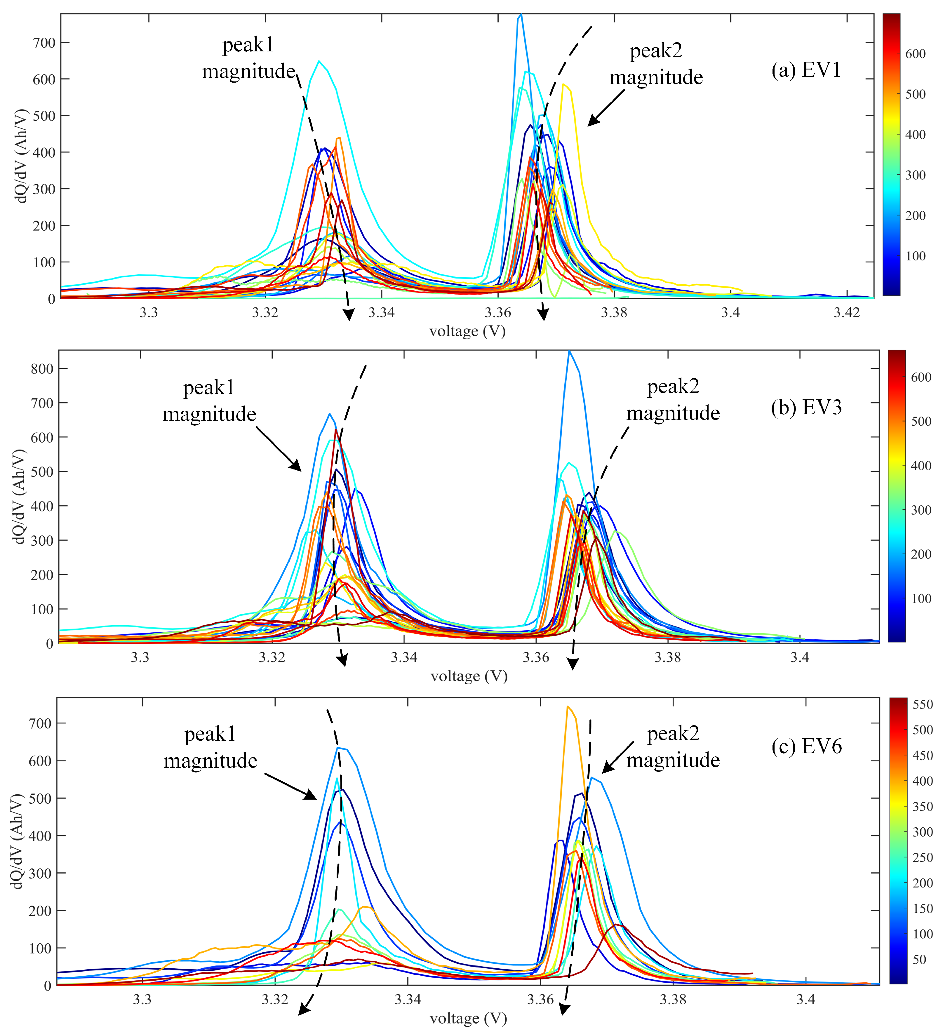
3.2.2. Incremental Capacity Analysis

To solve the capacity estimation of EVs with the degradation shown in Figure 2, only common used variables, such as current, voltage, and the SOC, are not enough. Inner knowledge of battery degradation should be further investigated. Incremental capacity analysis is always applied in the electrochemical modeling and capacity loss of LIBs. ICA is the change trends of charge quantity in the cell voltage, which means the cell’s ability to store charge quantity in every certain voltage period. Since the working voltage range of a cell is certain, the ability of quantity storage illustrates the available capacity.

Before the calculation of ICA, a cell inside the EV pack should have been selected to fetch the corresponding cell voltage to extract the ICA. However, the EV battery pack contains 36 cells. Hence, we statistically analyzed the maximum–voltage cell and the minimum–voltage cell marked by the battery management system (BMS) of the ten vehicles, and part of the maximum and minimum cell results of EV1 and EV7 are shown in Figure 4. To ensure the integration of the voltage plateau in the LFP cell and the corresponding peaks in the IC curves, the cell with the maximum voltage in every EV was selected because this cell may have been the first one to reach the charging cut–off voltage.

During its whole lifetime, EV7 contains totally 650 charging snippets in different DOCs, as shown in Figure 5, which contains enough degradation information for algorithm learning. To present the ICA relationship with battery degradation clearly, 55 snippets ranked from 1 to 55 according to the cycling increase were extracted from the 650 snippets by every 12 snippets with data preprocessing. Figure 6a,b are the charging voltage curves extracted from the selected LFP cell of EV7 and the corresponding IC curves, respectively. To highlight the ICA effects, only the two plateau regions of the LFP cell are plotted in Figure 6a, and the peaks in the IC curves shown in Figure 6b can be more clear. Figure 6a presents the shift in the voltage curves to the left region of the figure, and the lengths of the two plateau regions decrease with a cycling increase. Hence, the lengths of the two plateau regions are related to the battery degradation, and they can act as an indicator for RNN training. Then, the voltage plateau is transferred to the IC curves, as shown in Figure 6b, which demonstrates that the peaks’ magnitude in the IC curves decreases when the battery cycle increases. Hence, this work chooses the two peaks’ magnitude as the inputs of the proposed algorithm.

4. Physics-Informed Fractional-Order Recurrent Neural Network for Battery Degradation

The flowchart and framework for the whole structure of the PIRNN is shown in Figure 7. For battery degradation estimation, ICA with degradation information and a fractional-order gradient were both applied to a neural network, resulting in a physics-informed algorithm. The ICA inputs, network structure, and fractional-order gradient descent(FOGD) method will be introduced in the following sections, respectively.

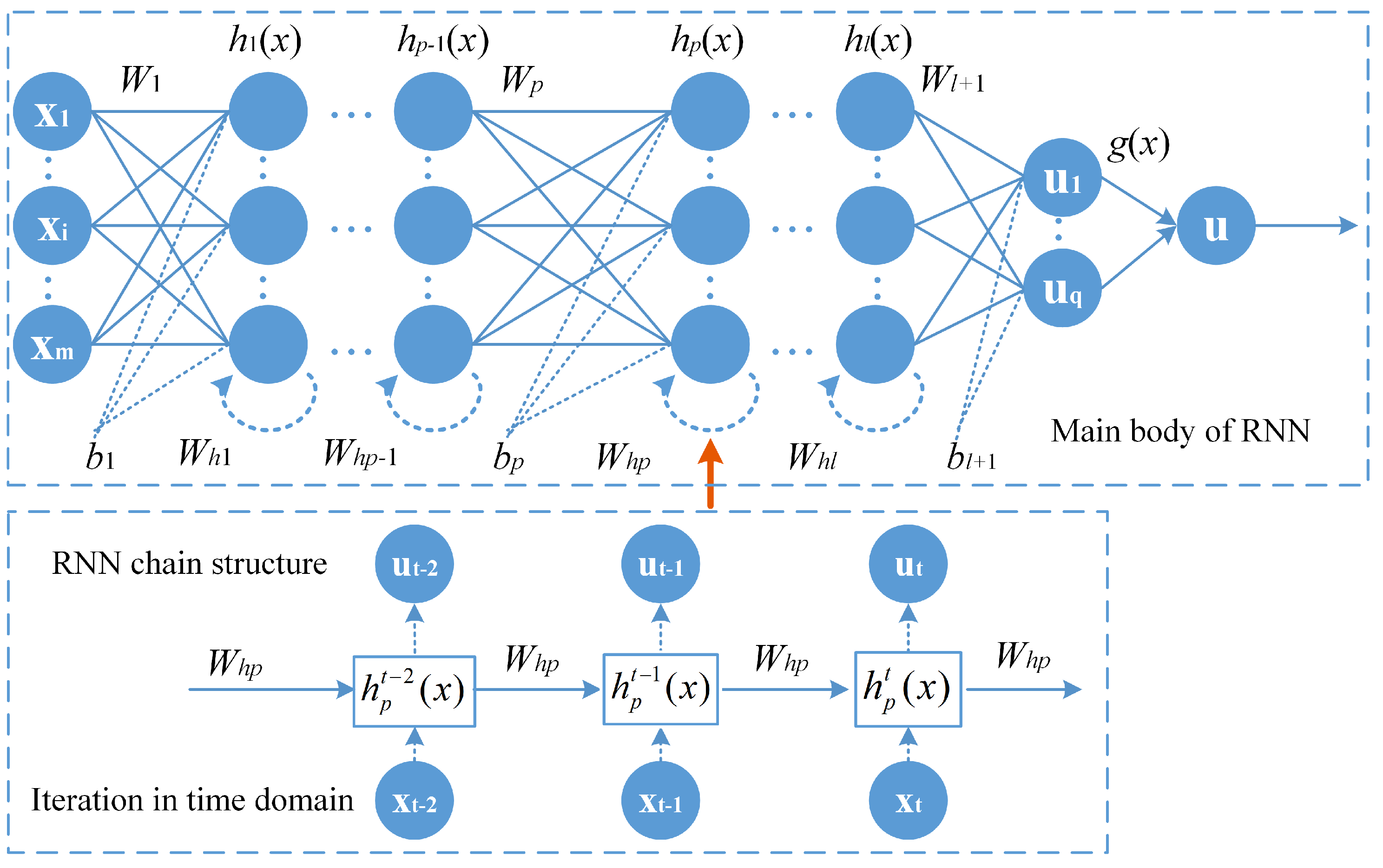
4.1. Physics-Informed Input with ICA Characteristics

The ICA curves of the ten EVs were extracted from the battery voltage curves, and part of the ICA curves are shown in Figure 8. For the LFP battery, the position and the length of the two plateau regions in the voltage curve shift when the battery cycles increase. From the battery mechanism aspect, the two plateau regions in the voltage curve correspond to the two peaks in the IC curves, which demonstrates the change in the loss of lithium inventory (LLI) or loss of active material (LAM) with battery aging. Hence, the length of the two plateau regions related to the battery degradation can be transferred to the magnitude of the two peaks, which are called the peak1 magnitude and peak2 magnitude in the following section, as marked in Figure 8. Although different cells may have different IC curves, as shown in Figure 8, the trends related to battery degradation are similar, and thus normalization was applied for every cell before they were input into the network.

4.2. Physics-Informed Structure of RNN

Besides the ICA characteristic, a physics-informed algorithm could be achieved from the structure aspect. The RNN in Figure 9 contains an input layer with m neurons, the hidden layers $(h_1,\dots ,h_{p-1},h_p,\dots ,h_l)$ with $n_p(p=1,2,\dots ,l)$ neurons, and an output layer with q neurons, respectively. Suppose that the training data are $({\mathbf{x}}_i,{\mathbf{u}}_i),i=1,2,\dots ,N$, where ${\mathbf{x}}_i={(x_{i1},x_{i2},\dots ,x_{im})}^{\mathrm{T}}$ is the input and ${\mathbf{u}}_i={(u_{i1},u_{i2},\dots ,u_{iq})}^{\mathrm{T}}$ is the ideal output. The vectors ${\mathbf{x}}_i$ and ${\mathbf{u}}_i$ are presented as x and u in the following context. In the chain structure of the RNN, $W_p$ and $b_p$ are the weight and bias matrix connecting the $(p-1)\mathrm{th}$ hidden layer to the $p\mathrm{th}$ hidden layer, $W_{hp}$ is the weight for the memory updates of the $p\mathrm{th}$ hidden layer, $g\left(x\right)$ is the activation function, and $L\left(g\right(x),u)$ is the loss function. Within the pre–set maximum epochs, the RNN went through forward propagation and backpropagation with the training dataset. The forward propagation starting from the input layer can be presented as

$$\left\{\begin{array}{c}{a}_p\left(x\right)=W_p{h}_{p-1}\left(x\right)+b_p,\hfill \\ h_p\left(x\right)=g\left(a_p\left(x\right)\right),p=1,2,\dots ,l\hfill \end{array}\right.$$

(10)

where $a_p\left(x\right)$ and $h_p\left(x\right)$ are the input and the output of the $p\mathrm{th}$ hidden layer, respectively. The weights $W_p$ and $W_{hp}$ and bias $b_p$ can be updated from the output layer to the hidden layers, and it always makes the weights $W_p=W_{hp}$ in real applications. The loss function $L\left(g\right(x),u)$ applied in this paper (also called the performance function) was selected as the mean square error (MSE), which is calculated as

$$L(g\left(x\right),u)={\displaystyle \frac{1}{N_{\mathrm{data}}}}{\sum }_{i=1}^{N_{\mathrm{data}}}{(u_i(x_i,t_i)-{\widehat{u}}_i)}^2$$

(11)

where $N_{\mathrm{data}}$ is the battery data amount and ${\widehat{u}}_i$ is the actual labels of the battery capacity.

4.3. Fractional-Order Gradient Descent Method

The fractional-order gradient descent (FOGD) method was proposed in our previous work [37]. Here, we present the results of the fractional-order gradient method, and further deduction processes can be found in [37]. Instead of integer–order gradients, the FOGD method employs fractional-order gradients with the loss function and weights updates. The FOGD for the updates of the weight $W_p$ is presented as

$$\begin{array}{cc}\hfill W_p^{k+1}& =W_p^k-\eta {·}_{W_p^0}{D}_{W_p^k}^{\alpha }L(g\left(x\right),y)\hfill \\ \hfill & =W_p^k-\eta ·{\displaystyle \frac{{\partial }^{\alpha }L(g\left(x\right),y)}{\partial {\left(W_p^k\right)}^{\alpha }}}\hfill \end{array}$$

(12)

Based on $a_p\left(x\right)=W_p{h}_{p-1}\left(x\right)+b_p$ in Equation (10) and the chain rule, Equation (12) is deduced as

$$W_p^{k+1}=W_p^k-\eta ·{\displaystyle \frac{\partial L\left(g\right(x),y)}{\partial a_p^k\left(x\right)}}·{\displaystyle \frac{{\partial }^{\alpha }{a}_p^k\left(x\right)}{\partial {\left(W_p^k\right)}^{\alpha }}}$$

(13)

where $\partial L\left(g\right(x),y)/\partial {\left(W_p^k\right)}^{\alpha }$ is the fractional-order gradient of the weight $W_p$ of the loss function $L\left(g\right(x),y)$ and $\eta$ is the learning rate (iteration step size). In Equation (13), the gradient of the input $a_p^k\left(x\right)$ to the loss function ($\partial L\left(g\right(x),y)/\partial a_p^k\left(x\right)$) can be obtained by

$$\left\{\begin{array}{cc}\hfill {\displaystyle \frac{\partial L\left(g\right(x),y)}{\partial h_p^k\left(x\right)}}=& W_{p+1}^k{\displaystyle \frac{\partial L\left(g\right(x),y)}{\partial a_{p+1}^k\left(x\right)}}\hfill \\ \hfill {\displaystyle \frac{\partial L\left(g\right(x),y)}{\partial a_p^k\left(x\right)}}=& {\displaystyle \frac{\partial L\left(g\right(x),y)}{\partial h_p^k\left(x\right)}}·g^{\prime }\left(a_p^k\left(x\right)\right)\hfill \\ \hfill =& W_{p+1}^k{\displaystyle \frac{\partial L\left(g\right(x),y)}{\partial a_{p+1}^k\left(x\right)}}·g^{\prime }\left(a_p^k\left(x\right)\right)\hfill \end{array}\right.$$

(14)

where $\partial L\left(g\right(x),y)/\partial h_p^k\left(x\right)$ and $\partial L\left(g\right(x),y)/\partial a_p^k\left(x\right)$ are the gradients of the output $h_p^k\left(x\right)$ and the input $a_p^k\left(x\right)$ of the $p\mathrm{th}$ hidden layer, respectively. ${\partial }^{\alpha }{a}_p^k\left(x\right)/\partial {\left(W_p^k\right)}^{\alpha }$ can be calculated by Equation (2). Hence, combining Equation (14) and the discrete Caputo definition in Equation (2), the fractional-order gradients of the weight $W_p$ of the loss function $L\left(g\right(x),y)$ can be deduced as

$${\displaystyle \frac{{\partial }^{\alpha }L(g\left(x\right),y)}{\partial {\left(W_p^k\right)}^{\alpha }}}={\displaystyle \frac{h_{p-1}^k\left(x\right)}{\mathrm{\Gamma }(2-\alpha )}}·{\displaystyle \frac{\partial L\left(g\right(x),y)}{\partial a_p^k\left(x\right)}}{\left(W_p^k-W_p^0\right)}^{1-\alpha }$$

(15)

where $W_p^0$ is the initial value of the weight $W_p$. Taking Equation (15) into Equation (13), we can obtain the FOGD method for backpropagation as

$$W_p^{k+1}=W_p^k-\eta ·{\displaystyle \frac{h_{p-1}^k\left(x\right)}{\mathrm{\Gamma }(2-\alpha )}}·{\displaystyle \frac{\partial L\left(g\right(x),y)}{\partial a_p^k\left(x\right)}}{\left(W_p^k-W_p^0\right)}^{1-\alpha }$$

(16)

where $\alpha$ is a fractional order that may be related to battery knowledge and sensitive to the training results. Equation Equation (16) is the basic equation of the FOGD method to update weights in the backpropagation process. With an updated equation (16), the procedure of the PIRNN with the maximum epoch ($E_{\max }$) can be concluded as follows.

• Step 1: perform initialization, with $W_p^0,p=1,2,\dots ,l$, $b_p^0$, the learning rate $l_r$, the fractional order $\alpha$, and so on.
• Step 2: obtain the battery dataset, and then preprocess the data (including extraction of inputs such as ICA magnitude) and divide the battery data into training, validating, and testing data.
• Step 3: perform the feedforward process, in a discrete form, with data flows in the PIRNN from the input layer to output layer, and then calculate the MSE ($ms{e}^k$).
• Step 4: perform the backpropagation process, starting from the output layer, to calculate the gradients between layers, and then update the weight $W_p$ and bias $b_p$ with (16).
• Step 5: Perform validation. Check if $ms{e}^k$ satisfies the target value or if the maximum epoch $E_{\max }$ is arrived at. If so, go to step 6; if not, go to step 3 and $epoch=epoch+1$.
• Step 6: If $ms{e}^k$ satisfies the target value of the loss function $ms{e}_{ref}^k$, the training process is completed, and capacity estimation and analysis should be conducted. Otherwise, if the maximum epoch $E_{\max }$ is arrived at, adjust the parameters and redo the procedure.

5. Algorithm Verification and Experimental Results

5.1. Experimental Setup

Experiments were conducted to demonstrate the effects of the proposed algorithm. The dataset with the labels of the ten EVs shown in Figure 2 was applied and divided into a training dataset, validation dataset, and testing dataset. The ten EVs contained a large amount of charging snippets in various DOC ranges, which were filtered into 5697 snippets, as shown in Table 1. A DOC histogram of the 5697 snippets is shown in Figure 10, which demonstrates that the dataset had high quality for network training, validation, and testing. Then, the 5697 snippets were divided into training, validation, and testing snippets in the ratio 0.8:0.05:0.15. With the partition of training, validation, and testing datasets, eight of the ten EVs (EV1–EV8) acted as the training dataset, almost half of EV9’s data were selected as the validation dataset, and the other half of EV9 and EV10 acted as the testing dataset. The selection of this partition was mainly according to the data length of the ten EVs in a time sequence, because 80% of the 5697 snippets were nearly the battery data of EV1–EV8, and we tended to make all EVs separate from each other. A large part (80%) of the EV snippets were considered training data to offer as many various battery degradation types of EVs as possible during the training process. Then, the algorithm could learn enough battery information for further testing estimation. Every snippet corresponded to a battery capacity value of an EV. Hence, the 15% testing part included 854 snippets of EVs, corresponding to 854 capacity points, which were enough for testing estimation. The validation part only needed a small section of data for the gradient threshold, and thus the validation section only took up 5%. Considering the ICA part, the inputs of the proposed algorithm were selected, as shown in

Table 2. The inputs of the proposed algorithm.

No.	1	2	3	4	5	6
Type	average current	start SOC	end SOC	DOC	start voltage	end voltage
No.	7	8	9	10	11	12
Type	mileage	Ah quantity	start temperature	end temperature	peak1 magnitude	peak2 magnitude

.

Besides the inputs, the algorithm parameters were pre–tuned for training performance. Here are the determined parameters of the proposed PIRNN, as shown in the following

Table 3. Algorithm parameters for training, validation, and testing.

Name	Value	Name	Value
state delays in PIRNN	1:2	hidden layer size	8
performance function	MSE	maximum epoch	3000
train function	FOGD	train–validation–test	0.8:0.05:0.15
learning rate $l_r$	0.0001	training goal	1
fractional order $\alpha$	0.8	validation times	50

. The main tuning parameters of the FOGD method were the learning rate $l_r$ and the fractional order $\alpha$.

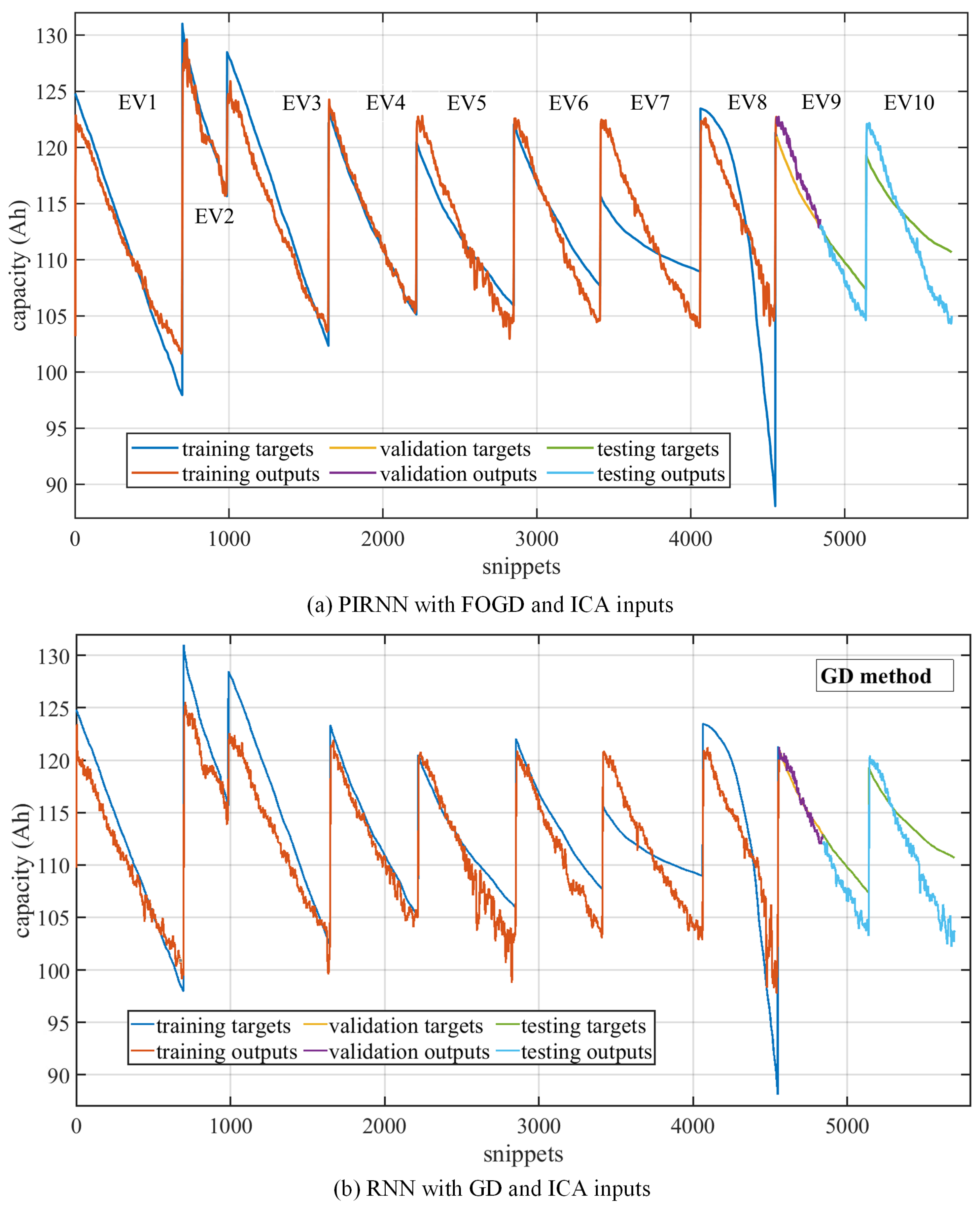
5.2. Estimation Results for Battery Degradation

We took the variables in Table 2 as the inputs, the parameters in Table 3 as the network parameters, and the capacity values as the output of the proposed algorithm; the estimation results are presented in this section. Figure 11 is the training process with the validation dataset, and the loss of the testing dataset is also shown in Figure 11. Since battery degradation is a key state changing with time, the training dataset, validation dataset, and testing dataset are plotted in a “pseudo” time–series sequence for the algorithm learning. The loss function is the MSE of the outputs, that is, the capacity estimation values. Figure 11 proves that the proposed algorithm could converge smoothly and rapidly with the fractional-order gradient method, and the loss could decrease into a small value (<10) less than 1/10 of the value of the loss in the beginning (180), which proves that the proposed PIRNN algorithm could learn the battery aging information with the fractional-order gradient decrease.

Figure 12 presents the estimation outputs of the proposed PIRNN algorithm, and the estimation results of the ten EVs are presented in a time series accompanied by the capacity labels shown in Figure 2. For comparison, the results of a conventional RNN with the GD method and also ICA inputs are presented with the results of the proposed PIRNN in Figure 12 and the following figures of the error and relative error. All parameters of the proposed PIRNN and conventional RNN with the GD method are the same except the fractional order. In the results of Figure 12, since the dataset of the ten EVs was divided into training–validation–testing as 0.8:0.05:0.15, eight of the ten EVs (EV1–EV8) act as the training dataset, almost half of EV9’s data is selected as the validation dataset, and the other half of EV9 and EV10 act as the testing dataset. Generally, the estimation results can fit most of the capacity of the ten EVs and track the fast degradation path of the LFP battery.

It should be noted that the transient variation in the shift points between every two EVs should not be taken as the estimation results of the proposed PIRNN algorithm. For example, the shift point between EV1 and EV2 caused a large capacity change from 98 Ah to 130 Ah, resulting a large amount of noise for the estimation output of the PIRNN in the beginning of EV2. Every point shown in Figure 12 presents a snippet among the 5697 snippets of the ten EVs, and the time range of every EV curve covers from 2018 to 2022, which is already a long running period. Although it still seems that the estimation performance of the algorithm in Figure 12 does not hold very well in every part of the capacity degradation curve, the estimation results can remain stable in most of the battery lifetime. Specifically, the training performance on EV7 and EV8 was the worst among the ten EVs, which may have been caused by the capacity change rates of EV7 and EV8, which varied from the other six training EVs. This also influenced the performance on the testing dataset, as shown in the right region of Figure 12, and the testing outputs turned out to be similar to those of the first six EVs.

To further illustrate the performance, the estimation errors (output labels) and the relative errors are also provided in Figure 13 and Figure 14, respectively. The relative errors were calculated by the absolute values of the output labels/labels, so the relative errors were calculated based on the battery aging labels rather than the rated capacity, which was a real-time error index.

Generally, the errors and relative errors in Figure 13 and Figure 14 demonstrate that the proposed algorithm could learn the battery’s physics-informed knowledge and control the errors within an acceptable range when the dataset held a similar fast degradation path. The errors of eight of the ten EVs shown in Figure 13 are lower than 5 Ah, which is small enough for a battery pack with a 130 Ah rated capacity. First of all, it should be noted that the shift points between every two EVs bring large and transient changes in the error values, such as the shift error between EV1 and EV2, EV3 and EV4, or EV8 and EV9, and the transient change in error should be considered noise rather than the estimation output. In the other hand, the error curves with shift points also prove that the proposed PIRNN can hold enough robustness with initial data noise. As shown in Figure 14, the relative errors of the first six EVs (EV1–EV6) and EV9 during the whole battery lifetime could be lower than 3%, which is also good enough for capacity estimation. However, in the end of the capacity curves of the ten EVs, especially EV5, EV6, and EV10, the proposed algorithm cannot learn the capacity trends as well as in the early stage, because the time interval between two snippets in this stage may be more than one month, and the EV battery may near the end of its lifetime, which makes it harder for algorithm to learn the trends. Moreover, EV7 and EV8 have batteries with faster degradation paths, and EV8 nearly has a dramatic drop in the end of its lifetime, so the proposed algorithm cannot catch the sudden drops by its current FOGD method.

Figure 12, Figure 13 and Figure 14 put the estimation results of the ten EVs together, which aims to show the general effectiveness of the proposed algorithm. To better illustrate the details, we extracted single estimation results for every EV from the ten EVs. Figure 15 shows the detailed results of EV4 in the training dataset, and Figure 16 is the comparison of EV6 in the training dataset and EV10 in the testing dataset. In Figure 15 and Figure 16, both capacity estimation outputs and the corresponding relative errors are provided, and the x–axes of the figures are the snippet numbers in all the 5697 obtained snippets of the ten EVs, so they do not start at 1. The results of EV4 in Figure 15 show the best fitting of capacity labels among the ten EVs. This does not mean that there is an over–fitting of EV4 data, because by comparing Figure 15 with Figure 12, the estimated outputs of the other nine EVs can be adjusted by the algorithm and the estimated degradation paths of the other nine EVs are various from each other. Meanwhile, in Figure 16, it can be observed that the estimated results in the end stage of the battery pack are not as accurate as those in the early stage. Thus, we find the critical point when the relative error exceeds 3%, which is also marked in Figure 16. For EV6 in the training dataset, the critical point happened at the time 9 October 2020, and the capacity label was 110.334 Ah with the SOH = 84.9%. For EV10 in the testing dataset, the critical point happened at the time 1 October 2020, and the capacity label was 112.179 Ah with the SOH = 86.3%. It can be seen that the estimation errors stayed under 3% until the battery lifetime reached around 85%; thus, this proves that the proposed algorithm could hold the estimation accuracy over three–quarters of the battery lifetime.

In this section, we present the estimation results and analysis of the proposed PIRNN algorithm for fast battery degradation estimation. The results show that the proposed algorithm could achieve a stable relative error < 3% for most of the ten EVs over three–quarters of the battery lifetime. The convergence process also showed that the proposed algorithm could learn the battery information through the IC inputs and FOGD method. However, the estimation accuracy decreased at the end of the battery lifetime and should be improved by embedding further physical information of the battery. Moreover, the performance on the battery with a dramatic degradation rate should be improved by introducing other physical inner degradation variables. It should be noted that all ten EVs collected in the dataset had a battery with fast degradation rather than a power–law trend, which may already make it harder to conduct capacity estimation in realistic operation conditions.

6. Conclusions

This paper proposes a physics-informed method for a fractional-order recurrent neural network to conduct battery capacity estimation, especially for a battery with fast degradation. A characteristic extracted from ICA was firstly applied to enhance the learning of the battery’s inner information and the algorithm interpretability. And, the fractional-order gradient descent method was also applied to accelerate the training process of the proposed algorithm. Hence, a fractional-order recurrent neural network with a physics-informed method was designed for battery capacity estimation. Specifically, the investigated battery dataset in this paper was from the LFP batteries of ten EVs with fast degradation, which is different from typical power–law capacity aging. The proposed algorithm was directly verified on the realistic sampled data and could realize a relative error < 3% for most of the ten EVs over three–quarters of the battery lifetime. The results show that the proposed algorithm could achieve stable performance in the fast degradation estimation when the batteries held similar degradation trends. The results prove that the research direction of encoding battery knowledge by the physics-informed method is worthy of investigation. However, other, more inner physical or even electrochemical variables could be added to enhance the physics-informed degree of machine learning. Moreover, other types of machine learning can also be considered to achieve better performance in further investigations.

References

1. Roman, D.; Saxena, S.; Robu, V.; Pecht, M.; Flynn, D. Machine learning pipeline for battery state-of-health estimation. Nat. Mach. Intell. 2021, 3, 447–456. [Google Scholar] [CrossRef]
2. Zhai, Q.; Jiang, H.; Long, N.; Kang, Q.; Meng, X.; Zhou, M.; Yan, L.; Ma, T. Machine learning for full lifecycle management of lithium-ion batteries. Renew. Sustain. Energy Rev. 2024, 202, 114647. [Google Scholar] [CrossRef]
3. Lai, X.; Yi, W.; Cui, Y.; Qin, C.; Han, X.; Sun, T.; Zhou, L.; Zheng, Y. Capacity estimation of lithium-ion cells by combining model-based and data-driven methods based on a sequential extended Kalman filter. Energy 2021, 216, 119233. [Google Scholar] [CrossRef]
4. Sulzer, V.; Mohtat, P.; Aitio, A.; Lee, S.; Yeh, Y.T.; Steinbacher, F.; Khan, M.U.; Lee, J.W.; Siegel, J.B.; Stefanopoulou, A.G.; et al. The challenge and opportunity of battery lifetime prediction from field data. Joule 2021, 5, 1934–1955. [Google Scholar] [CrossRef]
5. Schindler, M.; Sturm, J.; Ludwig, S.; Schmitt, J.; Jossen, A. Evolution of initial cell-to-cell variations during a three-year production cycle. ETransportation 2021, 8, 100102. [Google Scholar] [CrossRef]
6. Su, L.; Wu, M.; Li, Z.; Zhang, J. Cycle life prediction of lithium-ion batteries based on data-driven methods. ETransportation 2021, 10, 100137. [Google Scholar] [CrossRef]
7. Hong, J.; Wang, Z.; Chen, W.; Wang, L.; Lin, P.; Qu, C. Online accurate state of health estimation for battery systems on real-world electric vehicles with variable driving conditions considered. J. Clean. Prod. 2021, 294, 125814. [Google Scholar] [CrossRef]
8. Yang, H.; Wang, P.; An, Y.; Shi, C.; Sun, X.; Wang, K.; Zhang, X.; Wei, T.; Ma, Y. Remaining useful life prediction based on denoising technique and deep neural network for lithium-ion capacitors. ETransportation 2020, 5, 100078. [Google Scholar] [CrossRef]
9. How, D.N.; Hannan, M.; Lipu, M.H.; Ker, P.J. State of charge estimation for lithium-ion batteries using model-based and data-driven methods: A review. IEEE Access 2019, 7, 136116–136136. [Google Scholar] [CrossRef]
10. Lipu, M.H.; Hannan, M.; Hussain, A.; Ayob, A.; Saad, M.H.; Karim, T.F.; How, D.N. Data-driven state of charge estimation of lithium-ion batteries: Algorithms, implementation factors, limitations and future trends. J. Clean. Prod. 2020, 277, 124110. [Google Scholar] [CrossRef]
11. Wang, Y.; Wang, L.; Li, M.; Chen, Z. A review of key issues for control and management in battery and ultra-capacitor hybrid energy storage systems. ETransportation 2020, 4, 100064. [Google Scholar] [CrossRef]
12. Chen, Y.; Zhang, H.; Hong, J.; Hou, Y.; Yang, J.; Zhang, C.; Ma, S.; Zhang, X.; Yang, H.; Liang, F.; et al. Lithium plating detection of lithium-ion batteries based on the improved variance entropy algorithm. Energy 2024, 299, 131574. [Google Scholar] [CrossRef]
13. Lipu, M.H.; Abd Rahman, M.; Mansor, M.; Rahman, T.; Ansari, S.; Fuad, A.M.; Hannan, M. Data driven health and life prognosis management of supercapacitor and lithium-ion battery storage systems: Developments, implementation aspects, limitations, and future directions. J. Energy Storage 2024, 98, 113172. [Google Scholar] [CrossRef]
14. Amiri, M.N.; Haakansson, A.; Burheim, O.S.; Lamb, J.J. Lithium-ion battery digitalization: Combining physics-based models and machine learning. Renew. Sustain. Energy Rev. 2024, 200, 114577. [Google Scholar] [CrossRef]
15. Zhao, J.; Feng, X.; Pang, Q.; Fowler, M.; Lian, Y.; Ouyang, M.; Burke, A.F. Battery safety: Machine learning-based prognostics. Prog. Energy Combust. Sci. 2024, 102, 101142. [Google Scholar] [CrossRef]
16. Zhu, J.; Wang, Y.; Huang, Y.; Bhushan Gopaluni, R.; Cao, Y.; Heere, M.; Mühlbauer, M.J.; Mereacre, L.; Dai, H.; Liu, X.; et al. Data-driven capacity estimation of commercial lithium-ion batteries from voltage relaxation. Nat. Commun. 2022, 13, 1–10. [Google Scholar] [CrossRef]
17. Tian, J.; Xiong, R.; Shen, W.; Lu, J.; Yang, X.G. Deep neural network battery charging curve prediction using 30 points collected in 10 min. Joule 2021, 5, 1521–1534. [Google Scholar] [CrossRef]
18. Ng, M.F.; Zhao, J.; Yan, Q.; Conduit, G.J.; Seh, Z.W. Predicting the state of charge and health of batteries using data-driven machine learning. Nat. Mach. Intell. 2020, 2, 161–170. [Google Scholar] [CrossRef]
19. Chen, Z.; Zhao, H.; Zhang, Y.; Shen, S.; Shen, J.; Liu, Y. State of health estimation for lithium-ion batteries based on temperature prediction and gated recurrent unit neural network. J. Power Sources 2022, 521, 230892. [Google Scholar] [CrossRef]
20. Jui, J.J.; Ahmad, M.A.; Molla, M.I.; Rashid, M.I.M. Optimal Energy Management Strategies for Hybrid Electric Vehicles: A Recent Survey of Machine Learning Approaches. J. Eng. Res. 2024, 12, 454–467. [Google Scholar] [CrossRef]
21. Das, K.; Kumar, R.; Krishna, A. Analyzing electric vehicle battery health performance using supervised machine learning. Renew. Sustain. Energy Rev. 2024, 189, 113967. [Google Scholar] [CrossRef]
22. El-Azab, H.A.I.; Swief, R.; El-Amary, N.H.; Temraz, H. Seasonal electric vehicle forecasting model based on machine learning and deep learning techniques. Energy AI 2023, 14, 100285. [Google Scholar] [CrossRef]
23. Abdolrasol, M.G.; Hussain, S.S.; Ustun, T.S.; Sarker, M.R.; Hannan, M.A.; Mohamed, R.; Ali, J.A.; Mekhilef, S.; Milad, A. Artificial neural networks based optimization techniques: A review. Electronics 2021, 10, 2689. [Google Scholar] [CrossRef]
24. Stanley, K.O.; Clune, J.; Lehman, J.; Miikkulainen, R. Designing neural networks through neuroevolution. Nat. Mach. Intell. 2019, 1, 24–35. [Google Scholar] [CrossRef]
25. Amari, S.i. Backpropagation and stochastic gradient descent method. Neurocomputing 1993, 5, 185–196. [Google Scholar] [CrossRef]
26. Abdulkadirov, R.; Lyakhov, P.; Nagornov, N. Survey of optimization algorithms in modern neural networks. Mathematics 2023, 11, 2466. [Google Scholar] [CrossRef]
27. Mok, R.; Ahmad, M.A. Smoothed functional algorithm with norm-limited update vector for identification of continuous-time fractional-order Hammerstein models. IETE J. Res. 2024, 70, 1814–1832. [Google Scholar] [CrossRef]
28. Zhang, S.; Xie, L. Grafting constructive algorithm in feedforward neural network learning. Appl. Intell. 2023, 53, 11553–11570. [Google Scholar] [CrossRef]
29. Ahmad, M.A.; Mustapha, N.M.Z.A.; Nasir, A.N.K.; Tumari, M.Z.M.; Ismail, R.M.T.R.; Ibrahim, Z. Using normalized simultaneous perturbation stochastic approximation for stable convergence in model-free control scheme. In Proceedings of the 2018 IEEE International Conference on Applied System Invention (ICASI), Chiba, Japan, 13–17 April 2018; IEEE: Piscataway, NJ, USA, 2018; pp. 935–938. [Google Scholar]
30. Liu, T.; Ghosal, P.; Balasubramanian, K.; Pillai, N. Towards understanding the dynamics of gaussian-stein variational gradient descent. In Proceedings of the 37th Conference on Neural Information Processing Systems (NeurIPS 2023), New Orleans, LO, USA, 10–16 December 2023; Volume 36. [Google Scholar]
31. Feng, X.; Merla, Y.; Weng, C.; Ouyang, M.; He, X.; Liaw, B.Y.; Santhanagopalan, S.; Li, X.; Liu, P.; Lu, L.; et al. A reliable approach of differentiating discrete sampled-data for battery diagnosis. ETransportation 2020, 3, 100051. [Google Scholar] [CrossRef]
32. Karniadakis, G.E.; Kevrekidis, I.G.; Lu, L.; Perdikaris, P.; Wang, S.; Yang, L. Physics-informed machine learning. Nat. Rev. Phys. 2021, 3, 422–440. [Google Scholar] [CrossRef]
33. Li, W.; Zhang, J.; Ringbeck, F.; Jöst, D.; Zhang, L.; Wei, Z.; Sauer, D.U. Physics-informed neural networks for electrode-level state estimation in lithium-ion batteries. J. Power Sources 2021, 506, 230034. [Google Scholar] [CrossRef]
34. Tian, J.; Xiong, R.; Lu, J.; Chen, C.; Shen, W. Battery state-of-charge estimation amid dynamic usage with physics-informed deep learning. Energy Storage Mater. 2022, 50, 718–729. [Google Scholar] [CrossRef]
35. Wang, Y.; Chen, Y.; Liao, X. State-of-art survey of fractional order modeling and estimation methods for lithium-ion batteries. Fract. Calc. Appl. Anal. 2019, 22, 1449–1479. [Google Scholar] [CrossRef]
36. Wang, Y.; Han, X.; Guo, D.; Lu, L.; Chen, Y.; Ouyang, M. Physics-informed recurrent neural networks with fractional-order constraints for the state estimation of lithium-ion batteries. Batteries 2022, 8, 148. [Google Scholar] [CrossRef]
37. Wang, Y.; Han, X.; Lu, L.; Chen, Y.; Ouyang, M. Sensitivity of fractional-order Recurrent Neural Network with Encoded physics-informed Battery Knowledge. Fractal Fract. 2022, 6, 640. [Google Scholar] [CrossRef]
38. Wang, F.; Zhai, Z.; Zhao, Z.; Di, Y.; Chen, X. Physics-informed neural network for lithium-ion battery degradation stable modeling and prognosis. Nat. Commun. 2024, 15, 4332. [Google Scholar] [CrossRef] [PubMed]
39. Marc, W. Efficient Numerical Methods for Fractional Differential Equations and Their Analytical Background. Ph.D. Dissertation, Technischen Universit at Braunschweig, Braunschweig, Germany, 2005. [Google Scholar]
40. Wang, B.; Liu, Z.; Li, S.E.; Moura, S.J.; Peng, H. State-of-charge estimation for lithium-ion batteries based on a nonlinear fractional model. IEEE Trans. Control Syst. Technol. 2016, 25, 3–11. [Google Scholar] [CrossRef]
41. Zhang, Q.; Shang, Y.; Li, Y.; Cui, N.; Duan, B.; Zhang, C. A novel fractional variable-order equivalent circuit model and parameter identification of electric vehicle Li-ion batteries. ISA Trans. 2020, 97, 448–457. [Google Scholar] [CrossRef] [PubMed]
42. Zou, C.; Hu, X.; Dey, S.; Zhang, L.; Tang, X. Nonlinear fractional-order estimator with guaranteed robustness and stability for lithium-ion batteries. IEEE Trans. Ind. Electron. 2017, 65, 5951–5961. [Google Scholar] [CrossRef]
43. Nasser-Eddine, A.; Huard, B.; Gabano, J.D.; Poinot, T. A two steps method for electrochemical impedance modeling using fractional order system in time and frequency domains. Control Eng. Pract. 2019, 86, 96–104. [Google Scholar] [CrossRef]
44. Wang, X.; Wei, X.; Zhu, J.; Dai, H.; Zheng, Y.; Xu, X.; Chen, Q. A review of modeling, acquisition, and application of lithium-ion battery impedance for onboard battery management. ETransportation 2021, 7, 100093. [Google Scholar] [CrossRef]
45. Song, D.; Gao, Z.; Chai, H.; Jiao, Z. An adaptive fractional-order extended Kalman filtering approach for estimating state of charge of lithium-ion batteries. J. Energy Storage 2024, 85, 111089. [Google Scholar] [CrossRef]
46. Zhang, J.; Xiao, B.; Niu, G.; Xie, X.; Wu, S. Joint estimation of state-of-charge and state-of-power for hybrid supercapacitors using fractional-order adaptive unscented Kalman filter. Energy 2024, 294, 130942. [Google Scholar] [CrossRef]
47. Hu, T.; He, Z.; Zhang, X.; Zhong, S. Finite-time stability for fractional-order complex-valued neural networks with time delay. Appl. Math. Comput. 2020, 365, 124715. [Google Scholar] [CrossRef]
48. Huang, Y.; Yuan, X.; Long, H.; Fan, X.; Cai, T. Multistability of fractional-order recurrent neural networks with discontinuous and nonmonotonic activation functions. IEEE Access 2019, 7, 116430–116437. [Google Scholar] [CrossRef]
49. Khan, S.; Ahmad, J.; Naseem, I.; Moinuddin, M. A novel fractional gradient-based learning algorithm for recurrent neural networks. Circuits Syst. Signal Process. 2018, 37, 593–612. [Google Scholar] [CrossRef]
50. Han, X.; Ouyang, M.; Lu, L.; Li, J.; Zheng, Y.; Li, Z. A comparative study of commercial lithium ion battery cycle life in electrical vehicle: Aging mechanism identification. J. Power Sources 2014, 251, 38–54. [Google Scholar] [CrossRef]
51. Guo, D.; Yang, G.; Feng, X.; Han, X.; Lu, L.; Ouyang, M. Physics-based fractional-order model with simplified solid phase diffusion of lithium-ion battery. J. Energy Storage 2020, 30, 101404. [Google Scholar] [CrossRef]
52. Guo, D.; Yang, G.; Han, X.; Feng, X.; Lu, L.; Ouyang, M. Parameter identification of fractional-order model with transfer learning for aging lithium-ion batteries. Int. J. Energy Res. 2021, 45, 12825–12837. [Google Scholar] [CrossRef]
Figure 1. Typical degradation curve of LiFeP O 4 (LFP) battery with mileage increasing.
Fractalfract 09 00091 g001
Figure 2. The battery capacity labels in battery dataset of the ten EVs.
Fractalfract 09 00091 g002
Figure 3. The fractional-order PNGV model of LIBs for physical battery information embedded in the PIRNN.
Fractalfract 09 00091 g003
Figure 4. The accumulated time distribution of the maximum–voltage cell marked by the battery management system (BMS) during all charging snippets of (a,c) EV1 and (b,d) EV7.
Fractalfract 09 00091 g004
Figure 5. The 650 charging voltage curves of the selected LFP cell (the cell with maximum voltage) in EV7 with degradation.
Fractalfract 09 00091 g005
Figure 6. The extracted voltage curves and incremental capacity (IC) curves of the selected LFP cell in EV7 during charging with degradation. (a) The extracted charging voltage curves with two extracted plateau regions; (b) the IC curves.
Fractalfract 09 00091 g006
Figure 7. The flowchart and framework of the proposed PIRNN for fast battery degradation.
Fractalfract 09 00091 g007
Figure 8. The IC curves and characteristics extracted from the IC curves of EV1, EV3, and EV6.
Fractalfract 09 00091 g008
Figure 9. The structure of the proposed fractional-order recurrent neural network.
Fractalfract 09 00091 g009
Figure 10. The histogram of the DOC of all inputs.
Fractalfract 09 00091 g010
Figure 11. The training process of the proposed fractional-order recurrent neural network with the physics-informed method.
Fractalfract 09 00091 g011
Figure 12. The capacity estimation results of the proposed fractional-order recurrent neural network with the physics-informed method, compared to a conventional RNN with the GD method.
Fractalfract 09 00091 g012
Figure 13. The estimation errors of the proposed fractional-order recurrent neural network with the physics-informed method, compared to a conventional RNN with the GD method.
Fractalfract 09 00091 g013
Figure 14. The relative errors of the proposed fractional-order recurrent neural network with the physics-informed method, compared to a conventional RNN with the GD method.
Fractalfract 09 00091 g014
Figure 15. Detailed estimation and relative error of EV4 in training dataset. (a) EV4 estimation results with labels. (b) EV4 relative error.
Fractalfract 09 00091 g015
Figure 16. Comparison of training results and testing results with EV6 and EV10. (a) EV6 estimation and relative error in training dataset. (b) EV10 estimation and relative error in testing data.
Fractalfract 09 00091 g016aFractalfract 09 00091 g016b