Article

Representation of Special Functions by Multidimensional A- and J-Fractions with Independent Variables

Faculty of Mathematics and Computer Science, Vasyl Stefanyk Precarpathian National University, 57 Shevchenko Str., 76018 Ivano-Frankivsk, Ukraine
*
Author to whom correspondence should be addressed.
Fractal Fract. 2025, 9(2), 89; https://doi.org/10.3390/fractalfract9020089
Submission received: 31 December 2024 / Revised: 26 January 2025 / Accepted: 26 January 2025 / Published: 28 January 2025

Abstract

The paper deals with the problem of representing special functions by branched continued fractions, particularly multidimensional A- and J-fractions with independent variables, which are generalizations of associated continued fractions and Jacobi continued fractions, respectively. A generalized Gragg’s algorithm is constructed that enables us to compute, by the coefficients of the given formal multiple power series, the coefficients of the corresponding multidimensional A- and J-fractions with independent variables. Presented below are numerical experiments for approximating some special functions by these branched continued fractions, which are similar to fractals.

1. Introduction

The problem of representing special functions arises, in particular, when solving various functional equations. It contributes to the development and implementation of effective methods and algorithms that are implemented until the construction of special software [1,2,3,4,5]. Currently, various tools are used to represent these functions, including the multidimensional generalization of continued fractions—branched continued fractions—as a special family of functions (see, [6,7,8,9,10,11,12,13,14]). The construction of the rational approximations of a special function is based on the correspondence between the approximants of the branched continued fraction and the formal multiple power series, which represents this function (see, [15,16]). Furthermore, the problem of constructing the corresponding branched continued fractions contributes to the emergence of their various structures (see, [17,18,19,20,21,22,23]).
In [24], Dmytro Bodnar introduced the so-called “branched continued fractions with independent variables”, which, by their structure, are a multidimensional analogue of the multiple power series. The correspondence properties of these branched continued fractions with polynomial elements are closely connected to the degree and form of these polynomials. Their types are essential in the analytical continuation of special functions through branched continued fractions [16,25,26,27]. Based on the classical algorithm [15,28], algorithms have been constructed that enable us to compute, by the coefficients of the formal multiple power series, the coefficients of the corresponding multidimensional C-, g-, S-, A-, and J-fractions with independent variables [16,29,30].
The paper considers the problem of representing special functions by multidimensional A- and J-fractions with independent variables, which are generalizations of associated continued fractions (or A-fractions) and Jacobi continued fractions (or J-fractions) [31], respectively.
In the analytical theory of continued fractions, the use of Gragg’s algorithm [32], which is based on Theorem 7.14 [28], is efficient for the constructed corresponding A- and J-fractions.
Let the coefficients of the formal power series
L ( z ) = 1 + c 1 z + c 2 z 2 + c 3 z 3 +
satisfy the conditions H n ( 1 ) 0 , n 1 , where H n ( 1 ) and n 1 , are Hankel determinants associated with L ( z ) . Then, the coefficients of the A-fraction
1 + p 1 z 1 + q 1 z p 2 z 2 1 + q 2 z p 3 z 2 1 + q 1 z  
corresponding to L ( z ) , can be computed as follows:
p k + 1 = σ k σ k 1 , q k + 1 = τ k 1 τ k , k 0 ,
where
σ k = r = 0 k b k , r c 2 k + 1 r , τ k = 1 σ k r = 0 k b k , r c 2 k + 2 r ,
and for 1 r k + 1 ,
b k + 1 , r = b k , r + q k + 1 b k , r 1 p k + 1 b k 1 , r 2 ,
with the initial conditions
σ 1 = b 0 , 0 = b k + 1 , 0 = 1 , τ 1 = b k 1 , 1 b k , k + 1 = 0 .
In this paper, we construct and study a generalization of the Gragg’s algorithm. First, in Section 2, we give the necessary definitions. Then, in Section 3, we construct a generalized Gregg’s algorithm and establish necessary and sufficient conditions for its existence (Theorems 1 and 2 for multidimensional A- and J-fractions with independent variables, respectively). Finally, in Section 4, we give examples of representing special functions by multidimensional A- and J-fractions with independent variables, which are similar to fractals.

2. Correspondence

2.1. Formal Multiple Power Series [15,16]

Formal multiple power series at  z = 0 . Let N be a fixed natural number, Z 0 be the set of non-negative integers, C be the set of complex numbers, Z 0 N = Z 0 × Z 0 × × Z 0 be the Cartesian product of N copies of the Z 0 , C N = C × C × × C be the Cartesian product of N copies of the C ,   k = ( k 1 , k 2 , , k N ) be an element of Z 0 N , and z = ( z 1 , z 2 , , z N ) be an element of C N . For k Z 0 N and z C N , put
k ! = k 1 ! k 2 ! k N ! , | k | = k 1 + k 2 + + k N , z k = z 1 k 1 z 2 k 2 z N k N .
A series of the form
L * ( z ) = | k | 0 c k z k ,
where c k C for | k | 0 is called a formal multiple power series at z = 0 . A set of formal multiple power series at z = 0 is denoted by L .
Let R ( z ) be a function holomorphic in a neighbourhood of the origin ( z = 0 ) . Let the mapping Λ : R ( z ) Λ ( R ) associate with R ( z ) its Taylor expansion in a neighbourhood of the origin. A sequence { R n ( z ) } of functions holomorphic at the origin is said to correspond at z = 0 to a formal multiple power series L * ( z ) if
lim n λ ( L * Λ ( R n ) ) = ,
where λ is the function defined as follows: λ : L Z 0 { } ; if L * ( z ) 0 , then λ ( L * ) = ; if L * ( z ) 0 then λ ( L * ) = m , where m is the smallest degree of homogeneous terms for which c k 0 , that is m = | k | .
If { R n ( z ) } corresponds at z = 0 to a formal multiple power series L * ( z ) , then the order of correspondence of R n ( z ) is defined as
ν n = λ ( L * Λ ( R n ) ) .
By the definition of λ , the series L * ( z ) and Λ ( R n ) agree for all homogeneous terms up to and including degree ( ν n 1 ) .
Formal multiple power series at  z = . A sequence of rational functions { R n ( z ) } is said to correspond at z = to a formal multiple power series
L * ( z ) = | k | 0 c k z k ,
where c k C , k 0 , if the sequence { R n ( 1 / w 1 , 1 / w 2 , , 1 / w N ) } corresponds to a formal multiple power series at w = 0 obtained from (1) by replacing z i with 1 / w i ,   1 i N .
A formal multiple power series (1) is said to be an asymptotic expansion of a function R ( z ) at z = , with respect to a region D in C N , if for every n 0 there exist ρ n > 0 and η n > 0 such that
R ( z ) | k | = 0 n c k z k η n k = 1 N 1 | z k | n + 1 , | z k | > ρ n , 1 k N , z D .
We denote this by
R ( z ) | k | 0 c k z k , z k , 1 k N .

2.2. Branched Continued Fractions [16,25]

Let i ( 0 ) = 0 , I 0 = { 0 } , and, for k 1 ,
I k = { i ( k ) : i ( k ) = ( i 1 , i 2 , , i k ) , 1 i p i p 1 , 1 p k , i 0 = N } .
Let { a i ( k ) } i ( k ) I k , k 1 , { b i ( k ) } i ( k ) I k , k 0 denote the ordered pair of sequences of complex numbers with a i ( k ) 0 for all i ( k ) I k , k 1 , and if for k 1 there exists a multi-index i ( k ) I k such that b i ( k ) = 0 , than b i ( k 1 ) , j 0 for 1 j i k 1 and j i k . Let the sequence { f k } is defined as follows:
f 0 = b 0 , f 1 = b 0 + i 1 = 1 N a i ( 1 ) b i ( 1 ) ,
f 2 = b 0 + i 1 = 1 N a i ( 1 ) b i ( 1 ) + i 2 = 1 i 1 a i ( 2 ) b i ( 2 ) , , f k = b 0 + i 1 = 1 N a i ( 1 ) b i ( 1 ) + i 2 = 1 i 1 a i ( 2 ) b i ( 2 ) +   + i k = 1 i k 1 a i ( k ) b i ( k ) +   , .
The ordered pair
{ a i ( k ) } i ( k ) I k , k 1 , { b i ( k ) } i ( k ) I k , k 0 , { f k } k 0
is the branched continued fraction with independent variables denoted by the symbol
b 0 + i 1 = 1 N a i ( 1 ) b i ( 1 ) + i 2 = 1 i 1 a i ( 2 ) b i ( 2 ) + i 3 = 1 i 2 a i ( 3 ) b i ( 3 ) +   .
The numbers a i ( k ) and b i ( k ) are called the elements of the branched continued fraction with independent variables, the relation a i ( k ) / b i ( k ) is called the kth partial quotient, and the value f k is called the kth approximant.
Let ( i 1 , i 2 , , i k , ) be a fixed infinite multi-index, such that 1 i k i k 1 for k 1 , where i 0 = N . The continued fraction
a i 1 b i 1 + a i 1 , i 2 b i 1 , i 2 + a i 1 , i 2 , i 3 b i 1 , i 2 , i 3 +  
is called the ( i 1 , i 2 , , i k , ) -branch of the branched continued fraction with independent variables (2).
Next, let e 0 = ( 0 , 0 , , 0 ) ,   e k = ( δ k , 1 , δ k , 2 , , δ k , N ) be a multi-index, where 1 k N , δ i , j is a Kronecker symbol. Let us introduce the following sets of multi-indices for k 1
E k = { e i ( k ) : e i ( k ) = e i 1 , i 2 , , i k = e i 1 + e i 2 + + e i k , i ( k ) I k }
and the mapping φ : I k E k , such that φ ( i ( k ) ) = e i ( k ) for all i ( k ) I k ,   k 1 . It can be shown that the mapping φ is bijective.
Multidimensional A-fraction with independent variables. A branched continued fraction with independent variables of the form
i 1 = 1 N p e i ( 1 ) z i 1 1 + q e i ( 1 ) z i 1 + i 2 = 1 i 1 ( 1 ) δ i 1 , i 2 p e i ( 2 ) z i 1 z i 2 1 + q e i ( 2 ) z i 2 + i 3 = 1 i 2 ( 1 ) δ i 2 , i 3 p e i ( 3 ) z i 2 z i 3 1 + q e i ( 3 ) z i 3 +   ,
where the p e i ( k ) C { 0 } ,   q e i ( k ) C , e i ( k ) E k , k 1 , is called a multidimensional A-fraction with independent variables. For each n 1 the nth approximant f n ( z ) of (3) is expressed by
f n ( z ) = i 1 = 1 N p e i ( 1 ) z i 1 1 + q e i ( 1 ) z i 1 + i 2 = 1 i 1 ( 1 ) δ i 1 , i 2 p e i ( 2 ) z i 1 z i 2 1 + q e i ( 2 ) z i 2 +   + i n = 1 i n 1 ( 1 ) δ i n 1 , i n p e i ( n ) z i n 1 z i n 1 + q e i ( n ) z i n .
A multidimensional A-fraction with independent variables (3) is said to correspond at z = 0 to a formal multiple power series L * ( z ) if its sequence of approximants { f n ( z ) } corresponds to L * ( z ) at z = 0 .
The following result was proved in ([16], Theorem 3.5), and for convenience, we present its proof.
Theorem 1.
Every multidimensional A-fraction with independent variables (3) with sequence of approximants { f n ( z ) } corresponds at z = 0 to a uniquely determined formal multiple power series
L ( z ) = | k | 1 c k z k ,
where c k C , | k | 1 . The order of correspondence of the nth approximant f n ( z ) is ( 2 n + 1 ) , n 0 , and hence the formal Taylor series at z = 0 of f n ( z ) has the form
f n ( z ) = | k | = 1 2 n c k z k + | k | 2 n + 1 γ k ( n ) z k , n 1 ,
where γ k ( n ) C ,   | k | 2 n + 1 , n 0 .
Proof. 
Let
Q e i ( n ) ( n ) ( z ) = 1 + q e i ( n ) z i n , e i ( n ) E n , n 1 ,
and
Q e i ( k ) ( n ) ( z ) = 1 + q e i ( k ) z i k + i k + 1 = 1 i k ( 1 ) δ i k , i k + 1 p e i ( k + 1 ) z i k z i k + 1 1 + q e i ( k + 1 ) z i k + 1 + i k + 2 = 1 i k + 1 ( 1 ) δ i k + 1 , i k + 2 p e i ( k + 2 ) z i k + 1 z i k + 2 1 + q e i ( k + 2 ) z i k + 2 +   + i n = 1 i n 1 ( 1 ) δ i n 1 , i n p e i ( n ) z i n 1 z i n 1 + q e i ( n ) z i n ,
where e i ( k ) E k , 0 k n 1 , n 1 . Then
f n ( z ) = i 1 = 1 N p e i ( 1 ) z i 1 Q e i ( 1 ) ( n ) ( z ) , n 1 .
Since the equality Q e i ( k ) ( n ) ( 0 ) = 1 holds for all i ( k ) E k , 1 k n , n 1 , then for each i ( k ) E k , 1 k n , n 1 , the finite branched continued fraction 1 / Q e i ( k ) ( n ) ( z ) at z = 0 has a formal multiple power series (5). Then, every nth approximant f n ( z ) ,   n 1 is a function holomorphic in origin, and hence, for each n 1 , let the formal multiple power series
f n ( z ) = k 1 γ k ( n ) z k ,
be the expansion of the approximant f n ( z ) at z = 0 .
Since
Q e i ( k ) ( n ) ( z ) 0 , i ( k ) E k , 1 k n , n 1 ,
then, using the well-known formula for the difference between two approximants of (3) (see [16] and also [33]), for n 1 and k 1 , we obtain
f n + k ( z ) f n ( z ) = i 1 = 1 N i 2 = 1 i 1 i n + 1 = 1 i n ( 1 ) n p e i ( 1 ) z i 1 r = 2 n + 1 ( 1 ) δ i k 1 , i k p e i ( k ) z i k 1 z i k r = 1 n + 1 Q e i ( r ) ( n + k ) ( z ) r = 1 n Q e i ( r ) ( n ) ( z )
in neighborhood of origin. Hence, for arbitrary n 1 and k 1 , we have
Λ ( f n + k ) Λ ( f n ) = | k | 2 n + 1 ( γ k ( n + k ) γ k ( n ) ) z k
in a neighborhood of z = 0 . So, for every n 1 and k 1
ν n = λ ( Λ ( f n + k ) Λ ( f n ) ) = 2 n + 1
and it tends monotonically to as n .
Thus, for each n 1 , k 1 , the relation γ k ( n + k ) = γ k ( n ) holds for any 1 | k | 2 n . The multidimensional A-fraction with independent variables (3) corresponds to the formal multiple power series (5), where c k = γ k ( [ | k | / 2 ] + 1 ) (here, [ · ] means the integer part of the number) for all k 0 , since
L ( z ) Λ ( f n ) = | k | 2 n + 1 ( γ k ( [ | k | / 2 ] + 1 ) γ k ( n ) ) z k
for each n 1 . Hence, the order of correspondence of the nth approximant f n ( z ) is ( 2 n + 1 ) and the formal multiple power series (6) is a formal Taylor series for f n ( z ) at z = 0 .
Let us prove that this L ( z ) is unique. Assume that the multidimensional A-fraction with independent variables (3) also corresponds to
P ( z ) = k 1 β k ( [ | k | / 2 ] + 1 ) z k
at z = 0 . Since for any n 1
P ( z ) Λ ( f n ) = | k | 2 n + 1 ( β k ( [ | k | / 2 ] + 1 ) γ k ( n ) ) z k ,
then β k ( [ | k | / 2 ] + 1 ) = γ k ( [ | k | / 2 ] + 1 ) for all k such that 1 | k | n and n 1 . That is, the L ( z ) is unique. □
The following results is true.
Theorem 2.
Let D be a domain containing the origin ( z = 0 ). Assume that a multidimensional A-fraction with independent variables (3) corresponds at z = 0 to a formal multiple power series (5) and converges uniformly on every compact subset of D to a function f ( z ) , holomorphic in the domain D . Then, the formal multiple power series (5) is the formal Taylor series at z = 0 of the function f ( z ) .
Proof. 
Since the sequence of approximants { f n ( z ) } of (3) converges uniformly on every compact subset of the domain D to a function f ( z ) holomorphic in D , then, by Weierstrass’ theorem (see [34]) for arbitrary k 0 , we have
| k | f n ( z ) z k | k | f ( z ) z k
on each compact subset of the domain D . In addition, by Theorem 1 for each n 1 , the Λ ( f n ) and L ( z ) agree for all homogeneous terms up to and including degree 2 n .
Thus, for any k 0 , we obtain
lim n | k | f n z k ( 0 ) = | k | f z k ( 0 ) = k ! c k ,
where k ! = k 1 ! k 2 ! k N ! .
Hence,
f ( z ) = k 1 | k | f z k ( 0 ) z k k ! = k 1 c k z k
for all z D . □
Note that the domain of convergence of the multidimensional A-fraction with independent variables (3) may be wider than the domain of convergence of the multiple power series (5). Then, the branched continued fraction (3) is the analytical continuation of the function represented by this series.
Multidimensional J-fraction with independent variables. A branched continued fraction with independent variables of the form
i 1 = 1 N p e i ( 1 ) q e i ( 1 ) + z i 1 + i 2 = 1 i 1 ( 1 ) δ i 1 , i 2 p e i ( 2 ) q e i ( 2 ) + z i 2 + i 3 = 1 i 2 ( 1 ) δ i 2 , i 3 p e i ( 3 ) q e i ( 3 ) + z i 3 +   ,
where p e i ( k ) , q e i ( k ) , e i ( k ) E k ,   k 1 , are complex numbers and, in addition, p e i ( k ) 0 ,   e i ( k ) E k , k 1 , is called a multidimensional J-fraction with independent variables.
A multidimensional J-fraction with independent variables (7) is said to correspond at z = to the formal multiple power series (1) if its sequence of approximants { f n * ( z ) } corresponds to L * ( z ) at z = .
Note that multidimensional J-fractions with independent variables are closely related to multidimensional A-fractions with independent variables.
Indeed, if we set z i = 1 / w i , 1 i N , in (3) and perform the equivalence transformation (see, [33]), setting ρ e i ( k ) = w i k ,   e i ( k ) E k , k 1 , then, as a result, we will arrive at a multidimensional J-fraction with independent variables.
Finally, note that a multidimensional J-fraction with independent variables (7) does not always exist that corresponds to the formal multiple power series (1) at z = . The necessary and sufficient conditions for the coefficients of the formal multiple power series will be given in the next section for multidimensional A-fractions with independent variables (3).

3. Branched Continued Fraction Construction

3.1. Generalized Gragg’s Algorithm

Let N 2 . Let us consider the formal multiple power series (5) and show step by step the process of constructing the multidimensional A-fraction with independent variables (3).
Step 1.1: Let c e i 1 0 for 2 i 1 N . Then, we can rewrite L ( z ) in the form
L ( z ) = P e 0 ( z 1 ) + i 1 = 2 N c e i 1 z i 1 R e i 1 ( z ) ,
where
P e 0 ( z 1 ) = n = 1 c n e 1 z 1 n , R e i 1 ( z ) = k 0 m a t h b f k j = 0 , i 1 + 1 j N c k + e i 1 c e i 1 z k .
Step 1.2: Let H e 1 ( n ) 0 for n 1 , where
H e 1 ( n ) = c e 1 c 2 e 1 c n e 1 c 2 e 1 c 3 e 1 c ( n + 1 ) e 1 c n e 1 c ( n + 1 ) e 1 c ( 2 n 1 ) e 1
(we note that here H e 1 ( n ) comprises the Hankel determinants (of dimension n) associated with the formal power series P e 0 ( z 1 ) ). By Gragg’s algorithm, there exist numbers p n e 1 and q n e 1 , n 1 , such that p n e 1 0 ,   n 1 , and
P e 0 ( z 1 ) = n = 1 c n e 1 z 1 n p e 1 z 1 1 + q e 1 z 1 p 2 e 1 z 1 2 1 + q 2 e 1 z 1 p 3 e 1 z 1 2 1 + q 3 e 1 z 1   = F e 0 ( z 1 ) ,
where the symbol ‘∼’ means the correspondence between P e 0 ( z 1 ) and F e 0 ( z 1 ) (at the origin). The coefficients p n e 1 and q n e 1 , n 1 , are given by the formulas
p ( n + 1 ) e 1 = σ n e 1 σ ( n 1 ) e 1 , q ( n + 1 ) e 1 = τ ( n 1 ) e 1 τ n e 1 , n 0 ,
where
σ n e 1 = r = 0 n c ( 2 n + 1 r ) e 1 B n e 1 ( r ) , τ n e 1 σ n e 1 = r = 0 n c ( 2 n + 2 r ) e 1 B n e 1 ( r ) ,
and for 1 r n + 1 ,
B ( n + 1 ) e 1 ( r ) = B n e 1 ( r ) + q ( n + 1 ) e 1 B n e 1 ( r 1 ) p ( n + 1 ) e 1 B ( n 1 ) e 1 ( r 2 )
with the initial conditions
σ e 1 = B 0 e 1 ( 0 ) = B ( n + 1 ) e 1 ( 0 ) = 1 , τ e 1 = B ( n 1 ) e 1 ( 1 ) = B n e 1 ( n + 1 ) = 0 .
Thus, we can write
L ( z ) F e 0 ( z 1 ) + i 1 = 2 N c e i 1 z i 1 R e i 1 ( z ) .
Step 1.3: Let H e i 1 ( n ) 0 for 2 i 1 N and n 1 , where
H e i 1 ( n ) = c e i 1 c 2 e i 1 c n e i 1 c e 2 e i 1 c 3 e i 1 c ( n + 1 ) e i 1 c n e i 1 c ( n + 1 ) e i 1 c ( 2 n 1 ) e i 1 .
By Gragg’s algorithm, for each 2 i 1 N , there exists numbers p n e i 1 and q n e i 1 , n 1 , such that p n e i 1 0 , n 1 , and
n = 1 c n e i 1 z i 1 n p e i 1 z i 1 1 + q e i 1 z i 1 p 2 e i 1 z i 1 2 1 + q 2 e i 1 z i 1 p 3 e i 1 z i 1 2 1 + q 3 e i 1 z i 1   .
The coefficients p n e i 1 and q n e i 1 , n 1 are given by the formulas
p ( n + 1 ) e i 1 = σ n e i 1 σ ( n 1 ) e i 1 , q ( n + 1 ) e i 1 = τ ( n 1 ) e i 1 τ n e i 1 , n 0 ,
where
σ n e i 1 = r = 0 n c ( 2 n + 1 r ) e i 1 B n e i 1 ( r ) , τ n e i 1 σ n e i 1 = r = 0 n c ( 2 n + 2 r ) e i 1 B n e i 1 ( r ) ,
and for 1 r n + 1 ,
B ( n + 1 ) e i 1 ( r ) = B n e i 1 ( r ) + q ( n + 1 ) e i 1 B n e i 1 ( r 1 ) p ( n + 1 ) e i 1 B ( n 1 ) e i 1 ( r 2 )
with the initial conditions
σ e i 1 = B 0 e i 1 ( 0 ) = B ( n + 1 ) e i 1 ( 0 ) = 1 , τ e i 1 = B ( n 1 ) e i 1 ( 1 ) = B n e i 1 ( n + 1 ) = 0 .
Since
c e i 1 = c e i 1 B 0 e i 1 ( 0 ) = σ 0 e i 1 σ e i 1 = p e i 1 , 2 i 1 N ,
we set p e i 1 = p e i 1 ,   2 i 1 N .
Thus,
L ( z ) F e 0 ( z 1 ) + i 1 = 2 N p e i 1 z i 1 R e i 1 ( z ) .
Step 1.4: For each 2 i 1 N by
R e i 1 ( z ) = | k | 0 m a t h b f k j = 0 , i 1 + 1 j N c k e i 1 z k
we denote a formal multiple power series reciprocal to R e i 1 ( z ) . The coefficients of (12) are uniquely determined by the recurrence relations
c k e i 1 = | r | = 1 | k | c k r e i 1 c r + e i 1 c e i 1 ,
where c 0 e i 1 = 1 ; moreover, c k e i 1 = 0 , if there exists an index j ,   1 j N , such that k j < 0 .
Thus, we can write
L ( z ) F e 0 ( z 1 ) + i 1 = 2 N p e i 1 z i 1 R e i 1 ( z ) .
The next construction of the multidimensional A-fraction with independent variables will be carried out using the ideas outlined in Steps 1.1–1.4.
Step 2.1: Let c e i 2 e i 1 0 for 2 i 2 i 1 and 2 i 1 N . In addition, for the formation of partial denominators of the multidimensional A-fraction with independent variables, we set the following conditions c n e i 2 e i 1 = 0 for 1 i 2 i 1 1 ,   2 i 1 N and n 1 . Then, for each 2 i 1 N , we can rewrite the formal multiple power series (12) in the form
R e i 1 ( z ) = 1 + c e i 1 e i 1 z i 1 + z i 1 P e i 1 ( z 1 ) + i 2 = 2 i 1 c e i ( 2 ) e i 1 z i 1 z i 2 R e i ( 2 ) ( z ) ,
where
P e i 1 ( z 1 ) = n = 1 c e i 1 + n e 1 e i 1 z 1 n , R e i ( 2 ) ( z ) = | k | 0 m a t h b f k j = 0 , i 2 + 1 j N c k + e i ( 2 ) e i 1 c e i ( 2 ) e i 1 z k .
Since
c e i 1 e i 1 = c 2 e i 1 c e i 1 = c 2 e i 1 B 0 e i 1 ( 0 ) σ 0 e i 1 = τ 0 e i 1 = q e i 1 , 2 i 1 N ,
we set q e i 1 = q e i 1 , 2 i 1 N .
Thus,
L ( z ) F e 0 ( z 1 ) + i 1 = 2 N p e i 1 z i 1 1 + q e i 1 z i 1 + z i 1 P e i 1 ( z 1 ) + i 2 = 2 i 1 c e i ( 2 ) e i 1 z i 1 z i 2 R e i ( 2 ) ( z ) .
Step 2.2: Let H e i 1 + e 1 e i 1 ( n ) 0 for 2 i 1 N and n 1 , where
H e i 1 + e 1 e i 1 ( n ) = c e i 1 + e 1 e i 1 c e i 1 + 2 e 1 e i 1 c e i 1 + n e 1 e i 1 c e i 1 + 2 e 1 e i 1 c e i 1 + 3 e 1 e i 1 c e i 1 + ( n + 1 ) e 1 e i 1 c e i 1 + n e 1 e i 1 c e i 1 + ( n + 1 ) e 1 e i 1 c e i 1 + ( 2 n 1 ) e 1 e i 1 .
By Gragg’s algorithm, for each 2 i 1 N there exist numbers p e i 1 + n e 1 and q e i 1 + n e 1 , n 1 , such that p e i 1 + n e 1 0 , n 1 , and
n = 1 c e i 1 + n e 1 e i 1 z 1 n p e i 1 + e 1 z 1 1 + q e i 1 + e 1 z 1 p e i 1 + 2 e 1 z 1 2 1 + q e i 1 + 2 e 1 z 1 p e i 1 + 3 e 1 z 1 2 1 + q e i 1 + 3 e 1 z 1   = F e i 1 ( z 1 ) .
The coefficients p e i 1 + n e 1 and q e i 1 + n e 1 ,   n 1 are given by the formulas
p e i 1 + ( n + 1 ) e 1 = σ e i 1 + n e 1 e i 1 σ e i 1 + ( n 1 ) e 1 e i 1 , q e i 1 + ( n + 1 ) e 1 = τ e i 1 + ( n 1 ) e 1 e i 1 τ e i 1 + n e 1 e i 1 , n 0 ,
where
σ e i 1 + n e 1 e i 1 = r = 0 n c e i 1 + ( 2 n + 1 r ) e 1 e i 1 B e i 1 + n e 1 e i 1 ( r ) , τ e i 1 + n e 1 e i 1 σ e i 1 + n e 1 e i 1 = r = 0 n c e i 1 + ( 2 n + 2 r ) e 1 e i 1 B e i 1 + n e 1 e i 1 ( r ) ,
and for 1 r n + 1 ,
B e i 1 + ( n + 1 ) e 1 e i 1 ( r ) = B e i 1 + n e 1 e i 1 ( r ) + q e i 1 + ( n + 1 ) e 1 B e i 1 + n e 1 e i 1 ( r 1 ) p e i 1 + ( n + 1 ) e 1 B e i 1 + ( n 1 ) e 1 e i 1 ( r 2 )
with the initial conditions
σ e i 1 e 1 e i 1 = B e i 1 + 0 e 1 e i 1 ( 0 ) = B e i 1 + ( n + 1 ) e 1 e i 1 ( 0 ) = 1 , τ e i 1 e 1 e i 1 = B e i 1 + ( n 1 ) e 1 e i 1 ( 1 ) = B e i 1 + n e 1 e i 1 ( n + 1 ) = 0 .
Thus, we can write
L ( z ) F e 0 ( z 1 ) + i 1 = 2 N p e i 1 z i 1 1 + q e i 1 z i 1 + z i 1 F e i 1 ( z 1 ) + i 2 = 2 i 1 c e i ( 2 ) e i 1 z i 1 z i 2 R e i ( 2 ) ( z ) .
Step 2.3: Let H e i 1 + e i 2 e i 1 ( n ) 0 for 2 i 2 i 1 1 , 2 i 1 N and n 1 , where
H e i 1 + e i 2 e i 1 ( n ) = c e i 1 + e i 2 e i 1 c e i 1 + 2 e i 2 e i 1 c e i 1 + n e i 2 e i 1 c e i 1 + 2 e i 2 e i 1 c e i 1 + 3 e i 2 e i 1 c e i 1 + ( n + 1 ) e i 2 e i 1 c e i 1 + n e i 2 e i 1 c e i 1 + ( n + 1 ) e i 2 e i 1 c e i 1 + ( 2 n 1 ) e i 2 e i 1 .
Then, by Gragg’s algorithm, for each 2 i 2 i 1 1 and 2 i 1 N , there exist numbers p e i 1 + n e i 2 and q e i 1 + n e i 2 , n 1 , such that p e i 1 + n e i 2 0 , n 1 , and
n = 1 c e i 1 + n e i 2 e i 1 z i 2 n p e i 1 + e i 2 z i 2 1 + q e i 1 + e i 2 z i 2 p e i 1 + 2 e i 2 z i 2 2 1 + q e i 1 + 2 e i 2 z i 2 p e i 1 + 3 e i 2 z i 2 2 1 + q e i 1 + 3 e i 2 z i 2   .
The coefficients p e i 1 + n e i 2 and q e i 1 + n e i 2 , n 1 are given by the formulas
p e i 1 + ( n + 1 ) e i 2 = σ e i 1 + n e i 2 e i 1 σ e i 1 + ( n 1 ) e i 2 e i 1 , q e i 1 + ( n + 1 ) e i 2 = τ e i 1 + ( n 1 ) e i 2 e i 1 τ e i 1 + n e i 2 e i 1 for n 0 ,
where
σ e i 1 + n e i 2 e i 1 = r = 0 n c e i 1 + ( 2 n + 1 r ) e i 2 e i 1 B e i 1 + n e i 2 e i 1 ( r ) , τ e i 1 + n e i 2 e i 1 σ e i 1 + n e i 2 e i 1 = r = 0 n c e i 1 + ( 2 n + 2 r ) e i 2 e i 1 B e i 1 + n e i 2 e i 1 ( r ) ,
and for 1 r n + 1 ,
B e i 1 + ( n + 1 ) e i 2 e i 1 ( r ) = B e i 1 + n e i 2 e i 1 ( r ) + q e i 1 + ( n + 1 ) e i 2 B e i 1 + n e i 2 e i 1 ( r 1 ) p e i 1 + ( n + 1 ) e i 2 B e i 1 + ( n 1 ) e i 2 e i 1 ( r 2 )
with the initial conditions
σ e i 1 e i 2 e i 1 = B e i 1 + 0 e i 2 e i 1 ( 0 ) = B e i 1 + ( n + 1 ) e i 2 e i 1 ( 0 ) = 1 , τ e i 1 e i 2 e i 1 = B e i 1 + ( n 1 ) e i 2 e i 1 ( 1 ) = B e i 1 + n e i 2 e i 1 ( n + 1 ) = 0 .
Since for 2 i 2 i 1 1 , 2 i 1 N ,
c e i ( 2 ) e i 1 = c e i ( 2 ) e i 1 B e i 1 + 0 e i 2 e i 1 ( 0 ) = σ e i 1 + 0 e i 2 e i 1 σ e i 1 e i 2 e i 1 = p e i ( 2 ) ,
and for 2 i 1 N ,
c 2 e i 1 e i 1 = c e i 1 e i 1 c 2 e i 1 + c 3 e i 2 c e i 1 = c 3 e i 1 c e i 1 ( c 2 e i 1 ) 2 ( c e i 1 ) 2 = c 3 e i 1 + c 2 e i 1 q e i 1 B 0 e i 1 ( 0 ) c e i 1 = c 3 e i 1 B e i 1 ( 0 ) + c 2 e i 1 B e i 1 ( 1 ) c e i 1 B 0 e i 1 ( 0 ) = σ e i 1 σ 0 e i 1 = p 2 e i 1 ,
we set p e i ( 2 ) = p e i ( 2 ) , p 2 e i 1 = p 2 e i 1 ,   2 i 2 i 1 1 , 2 i 1 N . Thus,
L ( z ) F e 0 ( z 1 ) + i 1 = 2 N p e i 1 z i 1 1 + q e i 1 z i 1 + z i 1 F e i 1 ( z 1 ) + i 2 = 2 i 1 ( 1 ) δ i 1 , i 2 p e i ( 2 ) z i 1 z i 2 R e i ( 2 ) ( z ) .
Step 2.4: Let for each 2 i 2 i 1 and 2 i 1 N
R e i ( 2 ) ( z ) = | k | 0 m a t h b f k j = 0 , i 2 + 1 j N c k e i ( 2 ) z k
be reciprocal to the formal multiple power series R e i ( 2 ) ( z ) . It is known that the coefficients c k e i ( 2 ) , | k | 1 , k j = 0 ,   i k + 1 j N of (14) are uniquely determined by a recurrence formula
c k e i ( 2 ) = | r | = 1 | k | c k r e i ( 2 ) c r + e i ( 2 ) e i 1 c e i ( 2 ) e i 1 ,
where c 0 e i ( 2 ) = 1 ; moreover, c k e i ( 2 ) = 0 , if there exists an index j such that 1 j N and that k j < 0 . Then
L ( z ) F e 0 ( z 1 ) + i 1 = 2 N p e i 1 z i 1 1 + q e i 1 z i 1 + z i 1 F e i 1 ( z 1 ) + i 2 = 2 i 1 ( 1 ) δ i 1 , i 2 p e i ( 2 ) z i 1 z i 2 R e i ( 2 ) ( z ) .
Let us continue the construction of the multidimensional A-fraction with independent variables.
Step 3.1: Let c e i 2 + e i 3 e i ( 2 ) 0 for 1 i 3 i 2 ,   2 i 2 i 1 , 2 i 1 N , and c n e i 3 e i ( 2 ) = 0 for 1 i 3 i 2 1 ,   2 i 2 i 1 , 2 i 1 N , and n 1 . Then, for each 2 i 2 i 1 and 2 i 1 N , we have
R e i ( 2 ) ( z ) = 1 + c e i 2 e i ( 2 ) z i 2 + z i 2 P e i ( 2 ) ( z 1 ) + i 3 = 2 i 2 c e i 2 , i 3 e i ( 2 ) z i 2 z i 3 R e i ( 3 ) ( z ) ,
where
P e i ( 2 ) ( z 1 ) = n = 1 c e i 2 + n e 1 e i ( 2 ) z 1 n , R e i ( 3 ) ( z ) = | k | 0 k j = 0 , i 3 + 1 j N c k + e i 2 , i 3 e i ( 2 ) c e i 2 , i 3 e i ( 2 ) z k .
Since for 2 i 2 i 1 1 , 2 i 1 N ,
c e i 2 e i ( 2 ) = c e i 2 + e i ( 2 ) e i 1 c e i ( 2 ) e i 1 = c e i 1 + 2 e i 2 e i 1 B e i 1 + 0 e i 2 ( 0 ) σ e i 1 + 0 e i 2 e i 1 = τ e i 1 + 0 e i 2 e i 1 = q e i ( 2 ) ,
and for 2 i 1 N ,
c e i 1 2 e i 1 = c 3 e i 1 e i 1 c 2 e i 1 e i 1 = c 2 e i 1 e i 1 c 2 e i 1 + c e i 1 e i 1 c 3 e i 1 + c 4 e i 1 c e i 1 e i 1 c 2 e i 1 + c 3 e i 1 = c 2 e i 1 c e i 1 c 4 e i 1 c e i 1 c 3 e i 1 c 2 e i 1 c 3 e i 1 c e i 1 ( c 2 e i 1 ) 2 = c 2 e i 1 c e i 1 c 4 e i 1 + c 3 e i 1 q e i 1 B 0 e i 1 ( 0 ) c 3 e i 1 B e i 1 ( 0 ) + c 2 e i 1 q e i 1 B 0 e i 1 ( 0 ) = c 2 e i 1 c e i 1 c 4 e i 1 + c 3 e i 1 B e i 1 ( 1 ) c 3 e i 1 B e i 1 ( 0 ) + c 2 e i 1 B e i 1 ( 1 ) = c 2 e i 1 B 0 e i 1 ( 0 ) σ 0 e i 1 c 4 e i 1 B e i 1 ( 0 ) + c 3 e i 1 B e i 1 ( 1 ) σ e i 1 = τ 0 e i 1 τ e i 1 = q 2 e i 1 ,
we set q e i ( 2 ) = q e i ( 2 ) , q 2 e i 1 = q 2 e i 1 ,   2 i 2 i 1 1 , 2 i 1 N . Thus,
L ( z ) F e 0 ( z 1 ) + i 1 = 2 N p e i 1 z i 1 1 + q e i 1 z i 1 + z i 1 F e i 1 ( z 1 ) + i 2 = 2 i 1 ( 1 ) δ i 1 , i 2 p e i ( 2 ) z i 1 z i 2 1 + q e i ( 2 ) z i 2 + z i 2 P e i ( 2 ) ( z 1 ) + i 3 = 2 i 2 c e i 2 , i 3 e i ( 2 ) z i 2 z i 3 R e i ( 3 ) ( z ) .
Step 3.2: Let H e i 2 + e 1 e i ( 2 ) ( n ) 0 for 2 i 2 i 1 ,   2 i 1 N and n 1 , where
H e i 2 + e 1 e i ( 2 ) ( n ) = c e i 2 + e 1 e i ( 2 ) c e i 2 + 2 e 1 e i ( 2 ) c e i 2 + n e 1 e i ( 2 ) c e i 2 + 2 e 1 e i ( 2 ) c e i 2 + 3 e 1 e i ( 2 ) c e i 2 + ( n + 1 ) e 1 e i ( 2 ) c e i 2 + n e 1 e i ( 2 ) c e i 2 + ( n + 1 ) e 1 e i ( 2 ) c e i 2 + ( 2 n 1 ) e 1 e i ( 2 ) .
Then, by Gragg’s algorithm, for each 2 i 2 i 1 and 2 i 1 N , there exist numbers p e i ( 2 ) + n e 1 and q e i ( 2 ) + n e 1 , n 1 , such that p e i ( 2 ) + n e 1 0 for n 1 and
n = 1 c e i 2 + n e 1 e i ( 2 ) z 1 n p e i ( 2 ) + e 1 z 1 1 + q e i ( 2 ) + e 1 z 1 p e i ( 2 ) + 2 e 1 z 1 2 1 + q e i ( 2 ) + 2 e 1 z 1 p e i ( 2 ) + 3 e 1 z 1 2 1 + q e i ( 2 ) + 3 e 1 z 1   = F e i ( 2 ) ( z 1 ) .
The coefficients p e i ( 2 ) + n e 1 and q e i ( 2 ) + n e 1 ,   n 1 are given by the formulas for n 0 ,
p e i ( 2 ) + ( n + 1 ) e 1 = σ e i ( 2 ) + n e 1 e i ( 2 ) σ e i ( 2 ) + ( n 1 ) e 1 e i ( 2 ) , q e i ( 2 ) + ( n + 1 ) e 1 = τ e i ( 2 ) + ( n 1 ) e 1 e i ( 2 ) τ e i ( 2 ) + n e 1 e i ( 2 ) ,
where
σ e i ( 2 ) + n e 1 e i ( 2 ) = r = 0 n c e i ( 2 ) + ( 2 n + 1 r ) e 1 e i ( 2 ) B e i ( 2 ) + n e 1 e i ( 2 ) ( r ) , τ e i ( 2 ) + n e 1 e i ( 2 ) σ e i ( 2 ) + n e 1 e i ( 2 ) = r = 0 n c e i ( 2 ) + ( 2 n + 2 r ) e 1 e i ( 2 ) B e i ( 2 ) + n e 1 e i ( 2 ) ( r ) ,
and for 1 r n + 1 ,
B e i ( 2 ) + ( n + 1 ) e 1 e i ( 2 ) ( r ) = B e i ( 2 ) + n e 1 e i ( 2 ) ( r ) + q e i ( 2 ) + ( n + 1 ) e 1 B e i ( 2 ) + n e 1 e i ( 2 ) ( r 1 ) p e i ( 2 ) + ( n + 1 ) e 1 B e i ( 2 ) + ( n 1 ) e 1 e i ( 2 ) ( r 2 )
with the initial conditions
σ e i ( 2 ) e 1 e i ( 2 ) = B e i ( 2 ) + 0 e 1 e i ( 2 ) ( 0 ) = B e i ( 2 ) + ( n + 1 ) e 1 e i ( 2 ) ( 0 ) = 1 , τ e i ( 2 ) e 1 e i ( 2 ) = B e i ( 2 ) + ( n 1 ) e 1 e i ( 2 ) ( 1 ) = B e i ( 2 ) + n e 1 e i ( 2 ) ( n + 1 ) = 0 .
Thus,
L ( z ) F e 0 ( z 1 ) + i 1 = 2 N p e i 1 z i 1 1 + q e i 1 z i 1 + z i 1 F e i 1 ( z 1 ) + i 2 = 2 i 1 ( 1 ) δ i 1 , i 2 p e i ( 2 ) z i 1 z i 2 1 + q e i ( 2 ) z i 2 + z i 2 F e i ( 2 ) ( z 1 ) + i 3 = 2 i 2 c e i 2 , i 3 e i ( 2 ) z i 2 z i 3 R e i ( 3 ) ( z ) .
Step 3.3: Let H e i 2 + e i 3 e i ( 2 ) ( n ) 0 for 2 i 3 i 2 1 , 2 i 2 i 1 , 2 i 1 N and n 1 , where
H e i 2 + e i 3 e i ( 2 ) ( n ) = c e i 2 + e i 3 e i ( 2 ) c e i 2 + 2 e i 3 e i ( 2 ) c e i 2 + n e i 3 e i ( 2 ) c e i 2 + 2 e i 3 e i ( 2 ) c e i 2 + 3 e i 3 e i ( 2 ) c e i 2 + ( n + 1 ) e i 3 e i ( 2 ) c e i 2 + n e i 3 e i ( 2 ) c e i 2 + ( n + 1 ) e i 3 e i ( 2 ) c e i 2 + ( 2 n 1 ) e i 3 e i ( 2 ) .
Then, by Gragg’s algorithm, for each 2 i 3 i 2 1 ,   2 i 2 i 1 and 2 i 1 N there exist numbers p e i ( 2 ) + n e i 3 and q e i ( 2 ) + n e i 3 , n 1 , such that p e i ( 2 ) + n e i 3 0 , n 1 , and
n = 1 c e i 2 + n e i 3 e i ( 2 ) z i 3 n p e i ( 3 ) z i 3 1 + q e i ( 3 ) z i 3 p e i ( 2 ) + 2 e i 3 z i 3 2 1 + q e i ( 2 ) + 2 e i 3 z i 3 p e i ( 2 ) + 3 e i 3 z i 3 2 1 + q e i ( 2 ) + 3 e i 3 z i 3   .
The coefficients p e i ( 2 ) + n e i 3 and q e i ( 2 ) + n e i 3 , n 1 are given by the formulas for n 0 ,
p e i ( 2 ) + ( n + 1 ) e i 3 = σ e i ( 2 ) + n e i 3 e i ( 2 ) σ e i ( 2 ) + ( n 1 ) e i 3 e i ( 2 ) , q e i ( 2 ) + ( n + 1 ) e i 3 = τ e i ( 2 ) + ( n 1 ) e i 3 e i ( 2 ) τ e i ( 2 ) + n e i 3 e i ( 2 ) ,
where
σ e i ( 2 ) + n e i 3 e i ( 2 ) = r = 0 n c e i ( 2 ) + ( 2 n + 1 r ) e i 3 e i ( 2 ) B e i ( 2 ) + n e i 3 e i ( 2 ) ( r ) , τ e i ( 2 ) + n e i 3 e i ( 2 ) σ e i ( 2 ) + n e i 3 e i ( 2 ) = r = 0 n c e i ( 2 ) + ( 2 n + 2 r ) e i 3 e i ( 2 ) B e i ( 2 ) + n e i 3 e i ( 2 ) ( r ) ,
and for 1 r n + 1 ,
B e i ( 2 ) + ( n + 1 ) e i 3 e i ( 2 ) ( r ) = B e i ( 2 ) + n e i 3 e i ( 2 ) ( r ) + q e i ( 2 ) + ( n + 1 ) e i 3 B e i ( 2 ) + n e i 3 e i ( 2 ) ( r 1 ) p e i ( 2 ) + ( n + 1 ) e i 3 B e i ( 2 ) + ( n 1 ) e i 3 e i ( 2 ) ( r 2 )
with the initial conditions
σ e i ( 2 ) e i 3 e i ( 2 ) = B e i ( 2 ) + 0 e i 3 e i ( 2 ) ( 0 ) = B e i ( 2 ) + ( n + 1 ) e i 3 e i ( 2 ) ( 0 ) = 1 , τ e i ( 2 ) e i 3 e i ( 2 ) = B e i ( 2 ) + ( n 1 ) e i 3 e i ( 2 ) ( 1 ) = B e i ( 2 ) + n e i 3 e i ( 2 ) ( n + 1 ) = 0 .
Since for 2 i 3 i 2 1 , 2 i 2 i 1 ,   2 i 1 N ,
c e i 2 + e i 3 e i ( 2 ) = c e i 2 + e i 3 e i ( 2 ) B e i ( 2 ) + 0 e i 3 e i ( 2 ) ( 0 ) = σ e i ( 2 ) + 0 e i 3 e i ( 2 ) σ e i ( 2 ) e i 3 e i ( 2 ) = p e i ( 3 ) ,
and for 2 i 2 i 1 1 , 3 i 1 N ,
c 2 e i 2 e i ( 2 ) = c e i 2 e i ( 2 ) c e i 1 + 2 e i 2 e i 1 c e i ( 2 ) e i 1 c e i 1 + 3 e i 2 e i 1 c e i ( 2 ) e i 1 = ( c e i 1 + 2 e i 2 e i 1 ) 2 c e i ( 2 ) e i 1 c e i 1 + 3 e i 2 e i 1 ( c e i ( 2 ) e i 1 ) 2 = c e i 1 + 3 e i 2 e i 1 + c e i 1 + 2 e i 2 e i 1 q e i ( 2 ) c e i ( 2 ) e i 1 = c e i 1 + 3 e i 2 e i 1 B e i ( 2 ) e i 1 ( 0 ) + c e i 1 + 2 e i 2 e i 1 B e i ( 2 ) e i 1 ( 1 ) c e i ( 2 ) e i 1 B e i 1 + 0 e i 2 e i 1 ( 0 ) = σ e i ( 2 ) e i 1 σ e i 1 + 0 e i 2 e i 1 = p e i 1 + 2 e i 2 ,
(note that the coefficient c 2 e i 2 e i ( 2 ) is possible only if N 3 and, of course, the appearance of this coefficient here and similar others in the following steps depends on the number N), and for 2 i 1 N ,
c 2 e i 1 2 e i 1 = ( c 3 e i 1 e i 1 ) 2 c 2 e i 1 e i 1 c 4 e i 1 e i 1 ( c 2 e i 1 e i 1 ) 2 = c e i 1 ( c e i 1 c 3 e i 1 c 5 e i 1 + 2 c 2 e i 1 c 3 e i 1 c 4 e i 1 c 3 e i 1 3 c e i 1 c 4 e i 1 2 c 2 e i 1 2 c 5 e i 1 ) ( c e i 1 c 3 e i 1 c 2 e i 1 2 ) 2 = c 5 e i 1 + c 4 e i 1 ( q e i 1 + q 2 e i 1 ) + c 3 e i 1 ( q e i 1 q 2 e i 1 p 2 e i 1 ) c 3 e i 1 + c 2 e i 1 q e i 1 B 0 e i 1 ( 0 ) = c 5 e i 1 B 2 e i 1 ( 0 ) + c 4 e i 1 B 2 e i 1 ( 1 ) + c 3 e i 1 B 2 e i 1 ( 2 ) c 3 e i 1 B e i 1 ( 0 ) + c 2 e i 1 B e i 1 ( 1 ) = σ 2 e i 1 σ e i 1 = p 3 e i 1 ,
we put p e i ( 3 ) = p e i ( 3 ) , 2 i 3 i 2 1 ,   2 i 2 i 1 , 2 i 1 N ;   p e i 1 + 2 e i 2 = p e i 1 + 2 e i 2 ,   2 i 3 i 2 1 , 3 i 1 N ;   p 3 e i 1 = p 3 e i 1 , 2 i 1 N .
Thus,
L ( z ) F e 0 ( z 1 ) + i 1 = 2 N p e i 1 z i 1 1 + q e i 1 z i 1 + z i 1 F e i 1 ( z 1 ) + i 2 = 2 i 1 ( 1 ) δ i 1 , i 2 p e i ( 2 ) z i 1 z i 2 1 + q e i ( 2 ) z i 2 + z i 2 F e i ( 2 ) ( z 1 ) + i 3 = 2 i 2 ( 1 ) δ i 2 , i 3 p e i ( 3 ) z i 2 z i 3 R e i ( 3 ) ( z ) .
Step 3.4: We obtain
L ( z ) F e 0 ( z 1 ) + i 1 = 2 N p e i 1 z i 1 1 + q e i 1 z i 1 + z i 1 F e i 1 ( z 1 ) + i 2 = 2 i 1 ( 1 ) δ i 1 , i 2 p e i ( 2 ) z i 1 z i 2 1 + q e i ( 2 ) z i 2 + z i 2 F e i ( 2 ) ( z 1 ) + i 3 = 2 i 2 ( 1 ) δ i 2 , i 3 p e i ( 3 ) z i 2 z i 3 R e i ( 3 ) ( z ) ,
where for each 2 i 3 i 2 , 2 i 2 i 1 , and 2 i 1 N ,
R e i ( 3 ) ( z ) = | k | 0 k j = 0 , i 3 + 1 j N c k e i ( 3 ) z k
is reciprocal to the R e i ( 3 ) ( z ) . The coefficients of (15) are calculated as follows
c k e i ( 3 ) = | r | = 1 | k | c k r e i ( 3 ) c r + e i 2 , i 3 e i ( 2 ) c e i 2 , i 3 e i ( 2 ) ,
where c 0 e i ( 3 ) = 1 ; moreover, c k e i ( 3 ) = 0 , if there exists an index j such that 1 j N and k j < 0 .
The further construction of the multidimensional A-fraction with independent variables (3) consists of gradually applying steps similar to Steps 2.1–2.4 to all formal multiple power series in the denominators of the ending partial quotients of the finite branches of the branched continued fraction.
As a result, computing the coefficients c k e i 1 , | k | 1 ,   k j = 0 , i 1 + 1 j N , and 2 i 1 N , using the recurrence Formula (13), and the coefficients c k e i ( k ) , | k | 1 ,   k j = 0 , i k + 1 j N , k 2 , 2 i p i p 1 , and 1 p k , using the recurrence formula
c k e i ( k ) = | r | = 1 | k | c k r e i ( k ) c r + e i k 1 , i k e i ( k 1 ) c e i k 1 , i k e i ( k 1 ) ,
where c 0 e i ( k ) = 1 ; moreover, c k e i ( k ) = 0 if there exists an index j ,   1 j N , such that k j < 0 , provided that for 1 i 1 N and n 1
H e i 1 ( n ) 0 ,
where H e i 1 ( n ) is as defined in (8), and provided that for each 1 i k + 1 i k 1 , 2 i p i p 1 , 1 p k , k 1 and n 1
c n e i k + 1 e i ( k ) = 0 , H e i k , i k + 1 e i ( k ) ( n ) 0 ,
where H e i k , i k + 1 e i ( k ) ( n ) is defined by
H e i k , i k + 1 e i ( k ) ( n ) = c e i k , i k + 1 e i ( k ) c e i k + 2 e i k + 1 e i ( k ) c e i k + n e i k + 1 e i ( k ) c e i k + 2 e i k + 1 e i ( k ) c e i k + 3 e i k + 1 e i ( k ) c e i k + ( n + 1 ) e i k + 1 e i ( k ) c e i k + n e i k + 1 e i ( k ) c e i k + ( n + 1 ) e i k + 1 e i ( k ) c e i k + ( 2 n 1 ) e i k + 1 e i ( k ) .
For the formal multiple power series (5), we obtain the multidimensional A-fraction with independent variables (3), where the p e i ( k ) and q e i ( k ) for all e i ( k ) E k , k 1 is defined by the following formulas:
p ( n + 1 ) e i 1 = σ n e i 1 σ ( n 1 ) e i 1 , q ( n + 1 ) e i 1 = τ ( n 1 ) e i 1 τ n e i 1 ,
where 1 i 1 N , n 0 , and σ n e i 1 ,   τ n e i 1 , n 1 , are defined by (9)–(11),
p e i ( k ) + ( n + 1 ) e i k + 1 = σ e i ( k ) + n e i k + 1 e i ( k ) σ e i ( k ) + ( n 1 ) e i k + 1 e i ( k ) , q e i ( k ) + ( n + 1 ) e i k + 1 = τ e i ( k ) + ( n 1 ) e i k + 1 e i ( k ) τ e i ( k ) + n e i k + 1 e i ( k ) ,
where 2 i p i p 1 , 1 p k , 1 i k + 1 i k 1 , k 1 , n 0 ,
σ e i ( k ) + n e i k + 1 e i ( k ) = r = 0 n c e i ( k ) + ( 2 n + 1 r ) e i k + 1 e i ( k ) B e i ( k ) + n e i k + 1 e i ( k ) ( r ) , τ e i ( k ) + n e i k + 1 e i ( k ) σ e i ( k ) + n e i k + 1 e i ( k ) = r = 0 n c e i ( k ) + ( 2 n + 2 r ) e i k + 1 e i ( k ) B e i ( k ) + n e i k + 1 e i ( k ) ( r ) ,
and for 1 r n + 1 ,
B e i ( k ) + ( n + 1 ) e i k + 1 e i ( k ) ( r ) = B e i ( k ) + n e i k + 1 e i ( k ) ( r ) + q e i ( k ) + ( n + 1 ) e i k + 1 B e i ( k ) + n e i k + 1 e i ( k ) ( r 1 ) p e i ( k ) + ( n + 1 ) e i k + 1 B e i ( k ) + ( n 1 ) e i k + 1 e i ( k ) ( r 2 )
with the initial conditions
σ e i ( 2 ) e i 3 e i ( 2 ) = B e i ( 2 ) + 0 e i 3 e i ( 2 ) ( 0 ) = B e i ( 2 ) + ( n + 1 ) e i 3 e i ( 2 ) ( 0 ) = 1 , τ e i ( 2 ) e i 3 e i ( 2 ) = B e i ( 2 ) + ( n 1 ) e i 3 e i ( 2 ) ( 1 ) = B e i ( 2 ) + n e i 3 e i ( 2 ) ( n + 1 ) = 0 .
Thus, we have constructed the recurrence algorithm for computing the coefficients of the multidimensional A-fraction with independent variables (3) in terms of the formal multiple power series (5).

3.2. Multidimensional A-Fraction with Independent Variables

Let us show that the constructed in Section 3.1 the multidimensional A-fraction with independent variables (3) corresponds at z = 0 to the formal multiple power series (5).
Using Formulas (13), (16), (19), and (20), we curtail (4) for n 1 .
Note that according to the described above algorithm for e 0 and for all e i ( k ) such that 2 i p i p 1 , 1 p k , and k 1 , the continued fraction
F e i ( k ) ( z 1 ) = p e i ( k ) + e 1 z 1 1 + q e i ( k ) + e 1 z 1 p e i ( k ) + 2 e 1 z 1 2 1 + q e i ( k ) + 2 e 1 z 1 p e i ( k ) + 3 e 1 z 1 2 1 + q e i ( k ) + 3 e 1 z 1  
corresponds at the origin to the formal power series
P e i ( k ) ( z 1 ) = r = 1 c e i k + r e 1 e i ( k ) z 1 r
and the order of correspondence is ν n = 2 n + 1 . It follows that for e 0 and for each e i ( k ) such that 2 i p i p 1 ,   1 p k , k 1 and for n 2 the finite continued fraction
F e i ( k ) ( n ) ( z 1 ) = p e i ( k ) + e 1 z 1 1 + p e i ( k ) + e 1 z 1 p e i ( k ) + 2 e 1 z 1 2 1 + q e i ( k ) + 2 e 1 z 1   p e i ( k ) + n e 1 z 1 2 1 + q e i ( k ) + n e 1 z 1
has formal power series expansion
P e i ( k ) ( n ) ( z 1 ) = r = 1 2 n c e i k + r e 1 e i ( k ) z 1 r + O ( z 1 2 n + 1 ) ,
where c r e 1 e 0 = c r e 1 for 1 r 2 n and n 1 ,   O ( z 1 p ) is a symbolic mark for some formal power series, whose minimal degree of terms is not less than p , p 3 .
Now, for n = 1 , we have
f 1 ( z ) = i 1 = 1 N p e i 1 z i 1 1 + q e i 1 z i 1 = i 1 = 1 N c e i 1 z i 1 1 + c e i 1 e i 1 z i 1 = i 1 = 1 N c e i 1 z i 1 1 + i 2 = 1 i 1 c e i 2 e i 1 z i 2 = i 1 = 1 N c e i 1 z i 1 1 + i 2 = 1 i 1 c e i ( 2 ) c e i 1 z i 2 + O ( z 2 ) = i 1 = 1 N c e i 1 z i 1 + i 1 = 1 N z i 1 i 2 = 1 i 1 c e i ( 2 ) z i 2 + O ( z 3 ) = | k | = 1 2 c k z k + O ( z 3 ) ,
where O ( z p ) is a symbolic mark for some formal multiple power series, whose minimal degree of homogeneous terms is not less than p , p 2 . Since
| k | = 1 2 c k z k + O ( z 3 ) | k | 1 c k z k = O ( z 3 ) ,
where O ( z p ) is a symbolic mark for some formal multiple power series, whose minimal degree of homogeneous terms is not less than p , p 3 , then f 1 ( z ) L ( z ) and the order of correspondence is ν 1 = 3 .
For n = 2 we can write
f 2 ( z ) = F e 0 ( 2 ) ( z 1 ) + i 1 = 2 N p e i 1 z i 1 1 + q e i 1 z i 1 + i 2 = 1 i 1 ( 1 ) δ i 1 , i 2 p e i ( 2 ) z i 1 z i 2 1 + q e i ( 2 ) z i 2 = P e 0 ( 2 ) ( z 1 ) + i 1 = 2 N c e i 1 z i 1 1 + c e i 1 e i 1 z i 1 + i 2 = 1 i 1 c e i ( 2 ) e i 1 z i 1 z i 2 1 + c e i 2 e i ( 2 ) z i 2 = P e 0 ( 2 ) ( z 1 ) + i 1 = 2 N c e i 1 z i 1 1 + c e i 1 e i 1 z i 1 + i 2 = 1 i 1 c e i ( 2 ) e i 1 z i 1 z i 2 1 + i 3 = 1 i 2 c e i 3 e i ( 2 ) z i 3 = P e 0 ( 2 ) ( z 1 ) + i 1 = 2 N c e i 1 z i 1 1 + c e i 1 e i 1 z i 1 + i 2 = 1 i 1 c e i ( 2 ) e i 1 z i 1 z i 2 1 + i 3 = 1 i 2 c e i ( 2 ) + e i 3 e i 1 c e i ( 2 ) e i 1 z i 3 + O ( z 2 ) = P e 0 ( 2 ) ( z 1 ) + i 1 = 2 N c e i 1 z i 1 1 + i 2 = 1 i 1 c e i 2 e i 1 z i 2 + i 2 = 1 i 1 z i 2 i 3 = 1 i 2 c e i 2 , i 3 e i 1 z i 3 + i 2 = 1 i 1 z i 2 i 3 = 1 i 2 z i 3 i 4 = 1 i 3 c e i ( 4 ) e i 1 e i 1 z i 4 + O ( z 3 ) = P e 0 ( 2 ) ( z 1 ) + i 1 = 2 N c e i 1 z i 1 1 + i 2 = 1 i 1 c e i ( 2 ) c e i 1 z i 2 + i 2 = 1 i 1 z i 2 i 3 = 1 i 2 c e i ( 3 ) c e i 1 z i 3 + i 2 = 1 i 1 z i 2 i 3 = 1 i 2 z i 3 i 4 = 1 i 3 c e i ( 4 ) c e i 1 z i 4 + O ( z 4 ) = | k | = 1 4 c k z k + O ( z 5 ) .
Since
| k | = 1 4 c k z k + O ( z 5 ) | k | 1 c k z k = O ( z 5 ) ,
then f 2 ( z ) L ( z ) and ν 2 = 5 .
Next, let n 3 be an arbitrary natural number. Then we obtain
f n ( z ) = F e 0 ( n ) ( z 1 ) + i 1 = 2 N p e i 1 z i 1 1 + q e i 1 z i 1 + z i 1 F e i 1 ( n 1 ) ( z 1 ) +   + i n = 1 i n 1 ( 1 ) δ i n 1 , i n p e i ( n ) z i n 1 z i n 1 + q e i ( n ) z i n = P e 0 ( n ) ( z 1 ) + i 1 = 2 N c e i 1 z i 1 1 + c e i 1 e i 1 z i 1 + z i 1 P e i 1 ( n 1 ) ( z 1 ) + i 2 = 2 i 1 c e i ( 2 ) e i 1 z i 1 z i 2 1 + c e i 2 e i ( 2 ) z i 2 + z i 2 P e i ( 2 ) ( n 2 ) ( z 1 ) +   + i n = 1 i n 1 c e i n 1 , i n e i ( n 1 ) z i n 1 z i n 1 + c e i n e i ( n ) z i n
= P e 0 ( n ) ( z 1 ) + i 1 = 2 N c e i 1 z i 1 1 + c e i 1 e i 1 z i 1 + z i 1 P e i 1 ( n 1 ) ( z 1 ) +   + i n = 1 i n 1 c e i n 1 , i n e i ( n 1 ) z i n 1 z i n 1 + i n + 1 = 1 i n c e i n + 1 e i ( n ) z i n + 1 = P e 0 ( n ) ( z 1 ) + i 1 = 2 N c e i 1 z i 1 1 + c e i 1 e i 1 z i 1 + z i 1 P e i 1 ( n 1 ) ( z 1 ) +   + i n = 1 i n 1 c e i n 1 , i n e i ( n 1 ) z i n 1 z i n 1 + i n + 1 = 1 i n c e i n 1 , i n , i n + 1 e i ( n 1 ) c e i n 1 , i n e i ( n 1 ) z i n + 1 + O ( z 2 ) .
Continuing this process on the final step, we obtain
f n ( z ) = P e 0 ( n ) ( z 1 ) + i 1 = 2 N c e i 1 z i 1 1 + i 2 = 1 i 1 c e i 2 e i 1 z i 2 + + i 2 = 1 i 1 z i 2 i 2 n 1 = 1 i 2 n 2 z i 2 n 1 i 2 n = 1 i 2 n 1 c e i ( 2 n ) e i 1 e i 1 z i 2 n + O ( z 2 n 1 ) .
From this we have
f n ( z ) = P e 0 ( n ) ( z 1 ) + i 1 = 2 N c e i 1 z i 1 1 + i 2 = 1 i 1 c e i ( 2 ) c e i 1 z i 2 + + i 2 = 1 i 1 z i 2 i 2 n 1 = 1 i 2 n 2 z i 2 n 1 i 2 n = 1 i 2 n 1 c e i ( 2 n ) c e i 1 z i 2 n + O ( z 2 n ) = | k | = 1 2 n c k z k + O ( z 2 n + 1 ) .
Since
| k | = 1 2 n c k z k + O ( z 2 n + 1 ) | k | 1 c k z k = O ( z 2 n + 1 ) ,
f n ( z ) L ( z ) and ν n = 2 n + 1 .
At last, from the arbitrariness of n, it follows that f n ( z ) L ( z ) for all n 1 and that the order of correspondence is ν n = 2 n + 1 . It follows that Λ ( f n ) and L ( z ) agree for all homogeneous terms up to and including degree 2 n . Since
lim n + ν n = lim n + 2 n + 1 = + ,
the multidimensional A-fraction with independent variables (3) corresponds at z = 0 to the formal multiple power series (5).
Thus, the following theorem is true.
Theorem 3.
The multidimensional A-fraction with independent variables (3) corresponds at z = 0 to the given formal multiple power series (5) if and only if the conditions (17) for 1 i 1 N , n 1 , and the conditions (18) for 1 i k + 1 i k 1 , 2 i p i p 1 , 1 p k , k 1 , n 1 are satisfied.
It follows from Theorems 1 and 2 in [29] that the conditions for the existence of the generalized Gragg’s algorithm are the same as for the algorithm in [29]. However, this algorithm provides a more convenient numerical procedure for computing the coefficients of multidimensional A-fractions with independent variables corresponding to a formal multiple power series.

3.3. Multidimensional J-Fraction with Independent Variables

Let us consider the formal multiple power series
L * ( w ) = | k | 1 c k w k ,
where c k C , k 1 , and the multidimensional J-fraction with independent variables
i 1 = 1 N p e i ( 1 ) q e i ( 1 ) + w i 1 + i 2 = 1 i 1 ( 1 ) δ i 1 , i 2 p e i ( 2 ) q e i ( 2 ) + w i 2 + i 3 = 1 i 2 ( 1 ) δ i 2 , i 3 p e i ( 3 ) q e i ( 3 ) + w i 3 +   ,
where p e i ( k ) , q e i ( k ) , and e i ( k ) E k ,   k 1 are complex numbers, herewith p e i ( k ) 0 ,   e i ( k ) E k , k 1 .
The following theorem summarizes the connections between multidimensional A- and J-fractions with independent variables (see also [29], Theorem 3). Its proof is a simple application of Theorem 1.
Theorem 4.
Let f n ( z ) ( f n * ( w ) ) denote the nth approximants, respectively, of the multidimensional A-fraction with independent variables (3) (multidimensional J-fraction with independent variables (22)), where z i = 1 / w i and 1 i N . In addition, let the multidimensional A-fraction with independent variables (3) corresponds to the formal multiple power series (5) at z = 0 . Then
(A) 
For any natural n , the equality f n ( z ) = f n * ( w ) is true.
(B) 
The formal expansion of the nth approximant f n * ( w ) in the multiple power series at w = has the form
f n * ( w ) = | k | = 1 2 n c k w k + | k | 2 n + 1 c k ( n ) w k , n 1 ,
where c k ( n ) C ,   | k | 2 n + 1 , and hence, the multidimensional J-fraction with independent variables (22) corresponds at w = to the formal multiple power series (21).
It follows from Theorem 3 that the generalized Gragg’s algorithm can also be used for computing the coefficients of multidimensional J-fractions with independent variables corresponding to a formal multiple power series.

4. Applications

In this section, we will give some applications of the above constructed algorithm.
The function of two variables
f ( z ) = arctan ( z 1 ) + arctan z 2 1 + z 2 arctan ( z 1 )
has a formal double power series at origin given by
L ( z ) = k = 1 ( 1 ) k + 1 2 k 1 z 1 2 k 1 + r = 1 ( 1 ) r + 1 2 r 1 s = 0 z 2 s + 1 k = 1 ( 1 ) k 2 k 1 z 1 2 k 1 s 2 r 1 .
Applying the recurrence algorithm constructed in Section 3, we obtain the following.
Step 1.1: We have
L ( z ) = k = 1 ( 1 ) k + 1 2 k 1 z 1 2 k 1 + z 2 1 z 1 z 2 1 3 z 2 2 + 1 3 z 1 3 z 2 + z 1 2 z 2 2 + z 1 z 2 3 + 1 5 z 2 4 1 5 z 1 5 z 2 2 3 z 1 4 z 2 2 4 3 z 1 3 z 2 3 2 z 1 2 z 2 4 z 1 z 2 5 1 7 z 2 6 + .
Steps 1.2 and 1.3: By Formula (19), we obtain (see also Table 1)
p 1 , 0 = p 0 , 1 = 1 , p k , 0 = p 0 , k = ( k 1 ) 2 ( 2 k 3 ) ( 2 k 1 ) , k 2 , q k , 0 = q 0 , k = 0 , k 0 .
Table 1. Results of algorithm applied to (23) on Steps 1.2 and 1.3 for i 1 = 1 , 2 .
n p ne i 1 q ne i 1 σ ne i 1 τ ne i 1 B ne i 1 ( 0 ) B ne i 1 ( 1 ) B ne i 1 ( 2 )
1 10
0 101
110 1 / 3 010
2 1 / 3 04/451/1511/31/3
3 4 / 15 0
Thus,
L ( z ) F 0 ( z 1 ) + z 2 1 z 1 z 2 1 3 z 2 2 + 1 3 z 1 3 z 2 + z 1 2 z 2 2 + z 1 z 2 3 + 1 5 z 2 4 1 5 z 1 5 z 2 2 3 z 1 4 z 2 2 4 3 z 1 3 z 2 3 2 z 1 2 z 2 4 z 1 z 2 5 1 7 z 2 6 + ,
where
F 0 ( z 1 ) = p 1 , 0 z 1 1 p 2 , 0 z 1 2 1 p 3 , 0 z 1 2 1   .
Step 1.4: Through the recurrence Formula (13), we obtain
L ( z ) F 0 ( z 1 ) + z 2 R 0 , 1 ( z ) ,
where
R 0 , 1 ( z ) = 1 + z 1 z 2 + 1 3 z 2 2 1 3 z 1 3 z 2 1 3 z 1 z 2 3 4 45 z 2 4 + 1 5 z 1 5 z 2 + 1 9 z 1 3 z 2 3 + 1 3 z 1 2 z 2 4 + 12 45 z 1 z 2 5 + 44 945 z 2 6 + .
Step 2.1: We have
L ( z 1 , z 2 ) F 0 ( z 1 ) + z 2 1 + z 2 k = 1 ( 1 ) k + 1 2 k 1 z 1 2 k 1 + z 2 2 3 R 0 , 2 ( z ) ,
where
R 0 , 2 ( z ) = 1 z 1 z 2 4 15 z 2 2 + 1 3 z 1 3 z 2 + z 1 2 z 2 2 + 12 15 z 1 z 2 3 + 44 315 z 2 4 + .
Steps 2.2 and 2.3: By Formula (20), we obtain (see also Table 2)
p 1 , 1 = 1 , p n , 1 = ( n 1 ) 2 ( 2 n 3 ) ( 2 n 1 ) , n 2 , q n , 1 = 0 , n 0 .
Table 2. Results of algorithm applied to (23) on Steps 2.2 and 2.3.
n p n , 1 q n , 1 σ n , 1 τ n , 1 B n , 1 ( 0 ) B n , 1 ( 1 ) B n , 1 ( 2 )
1 10
0 101
110 1 / 3 010
2 1 / 3 04/451/1511/31/3
3 4 / 15 0
Thus,
L ( z ) F 0 ( z 1 ) + z 2 1 + z 2 F 1 ( z 1 ) + z 2 2 3 R 0 , 2 ( z ) ,
where
F 1 ( z 1 ) = p 1 , 1 z 1 1 p 2 , 1 z 1 2 1 p 3 , 1 z 1 2 1   .
Step 2.4: Through the recurrence Formula (16), we obtain
L ( z ) F 0 ( z 1 ) + z 2 1 + z 2 F 1 ( z 1 ) + z 2 2 / 3 R 0 , 2 ( z ) ,
where
R 0 , 2 ( z ) = 1 + z 1 z 2 + 4 15 z 2 2 1 3 z 1 3 z 2 4 15 z 1 z 2 3 44 315 z 2 4 + .
And so on; at the end, we will obtain the corresponding two-dimensional A-fraction with independent variables of the form
F 0 ( z 1 ) + z 2 1 + z 2 F 1 ( z 1 ) + p 0 , 2 z 2 2 1 + z 2 F 2 ( z 1 ) + p 0 , 3 z 2 2 1 +   ,
where for k 0
F k ( z 1 ) = z 1 1 p 2 , k z 1 2 1 p 3 , k z 1 2 1   , p n , k = p 0 , n = ( n 1 ) 2 ( 2 n 3 ) ( 2 n 1 ) , n 2 .
In addition, we note that (25) converges in the domains
O = z C 2 : | z 1 | < 3 2 , | z 2 | < 6 4 , | z 1 z 2 | < 1 8
and
D = z C 2 : | arg ( z k ) | < π 2 , k = 1 , 2 ,
which follows from [35] and [36] (Theorem 5), respectively. Hence, it represents a single-valued branch of the analytic function (23) in the domain O D .
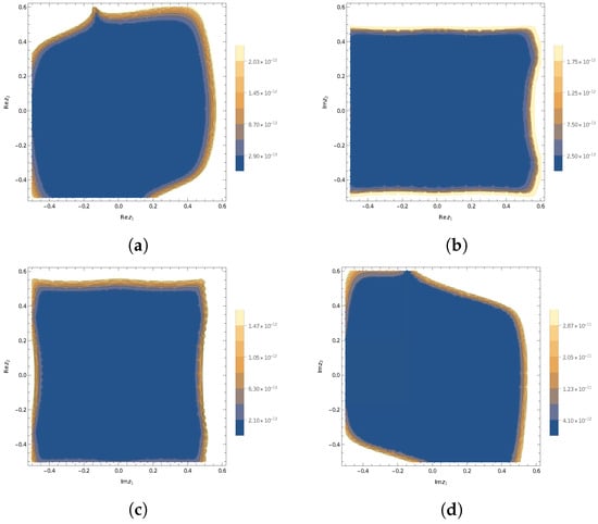
In Figure 1a,b, we can see the so-called “fork property” for a branched continued fraction with positive elements (see [33]). That is, the plots of the values of even (odd) approximations of (25) approach from below (above) the plot of the function (23). Figure 2a–d shows the plots, where the tenth approximant of (25) guarantees certain truncation error bounds for function (23).
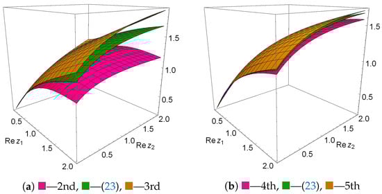
The numerical illustration of (24) and (25) is given in the Table 3. Here, we can see that the fifth approximant of (25) is eventually a better approximation to (23) than the fifth partial sum of (24) is.
Finally, consider the following function of two variables
ψ ( z ) = ψ ( z 1 ) + ψ ( z 2 + ψ ( z 1 ) ) = 0 t e t z 1 1 e t d t + 0 s 1 e s exp s z 2 s 0 t e t z 1 1 e t d t d s ,
where ψ ( . ) is the trigamma function (see [37]).
Using the asymptotic expansion for ψ ( . ) given in [37], we find the asymptotic representation for (26) as a formal double power series
ψ ( z ) k = 0 B k + z 1 k + 1 + r = 0 B r + z 2 r + 1 s = 0 k = 0 B k + z 1 k + 1 z 2 s r + 1 , z ,
where | arg ( z i ) | < π , i = 1 , 2 , and
B k + = 1 r = 0 k 1 k r B r + k r + 1 , k 0 ,
are the Bernoulli numbers. Then, by Theorem 3, using the algorithm from Section 3, we obtain the corresponding two-dimensional J-fraction with independent variables
i 1 = 1 2 p e i ( 1 ) q e i ( 1 ) + z i 1 + i 2 = 1 i 1 p e i ( 2 ) q e i ( 2 ) + z i 2 + i 3 = 1 i 2 p e i ( 3 ) q e i ( 3 ) + z i 3 +   ,
where
p e 1 + r e 2 = p e 2 = 1 , r 0 , p k e 1 + r e 2 = p k e 2 = ( k 1 ) 4 4 ( 2 k 3 ) ( 2 k 1 ) , k 2 , r 0 , q k e 1 + r e 2 = q k e 2 = 1 2 , k 1 , r 0 .
In addition, in [38], it is shown that (28) converges and, hence, represents the analytic function (26) in the domain
D ε = z C 2 : arg z k 1 2 < π 2 ε , k = 1 , 2 ,
where 0 < ε < π / 2 .
Plots of the values of the nth approximants of the two-dimensional J-fraction with independent variables (28) for function (26) are shown in Figure 3a,b. Figure 4a–d shows the plots, where the tenth approximant of (28) guarantees certain truncation error bounds for (26). The numerical illustration of (27) and (28) is given in the Table 4. Here, we have results similar to the results in the previous example.
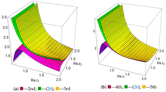
It should be noted that the two-dimensional A-fraction with independent variables (25) and two-dimensional J-fraction with independent variables (28) are similar to fractals.
The calculations and plots were performed using Wolfram Mathematica software 13.1.0.0 for Linux.

5. Conclusions

This paper concerns the representation of special functions by multidimensional A- and J-fractions with independent variables. The generalized Gragg’s algorithm is constructed and theorems are proved that provide necessary and sufficient conditions such that for a formal multiple power series there exist corresponding multidimensional A- and J-fractions with independent variables. Explicit formulas for the coefficients of these branched continued fraction are also given.
The obtained results can be used to construct approximate or exact analytical solutions to equations describing complex processes, for example, physics, chemistry, and engineering, thus providing a better and more meaningful understanding of the properties of processes and mechanisms.
The numerical experiments show, on the one hand, the efficiency of the proposed generalized Gragg’s algorithm and, on the other, the power and feasibility of the method in order to numerically approximate special functions from their formal multiple power series. In addition, they indicate the existence of wider domains of convergence multidimensional A- and J-fractions with independent variables, and hence, domains of analytical expansion of special functions. However, the problem of establishing them remains open. In [39,40], the truncation error bounds for these branched continued fractions were established; nevertheless, the problem of establishing them also remains open.

Author Contributions

Conceptualization, R.D.; investigation, R.D.; software, S.S.; writing—original draft, R.D.; writing—review & editing, R.D. and S.S.; project administration, R.D. All authors have read and agreed to the published version of the manuscript.

Funding

This research received no external funding.

Data Availability Statement

Data are contained within the article.

Acknowledgments

The authors were partially supported by the Ministry of Education and Science of Ukraine, project registration number 0122U000857.

Conflicts of Interest

The authors declare no conflicts of interest.

References

  1. Choi, J. Recent advances in special functions and their applications. Symmetry 2023, 15, 2159. [Google Scholar] [CrossRef]
  2. Exton, H. Multiple Hypergeometric Functions and Applications; Horwood, E., Ed.; Halsted Press: Chichester, UK, 1976. [Google Scholar]
  3. Milovanovic, G.; Rassias, M. (Eds.) Analytic Number Theory, Approximation Theory, and Special Functions; Springer: New York, NY, USA, 2014. [Google Scholar]
  4. Seaborn, J.B. Hypergeometric Functions and Their Applications; Springer: New York, NY, USA, 1991. [Google Scholar]
  5. Srivastava, H.M.; Karlsson, P.W. Multiple Gaussian Hypergeometric Series; Halsted Press: New York, NY, USA, 1985. [Google Scholar]
  6. Antonova, T.; Dmytryshyn, R.; Sharyn, S. Branched continued fraction representations of ratios of Horn’s confluent function H6. Constr. Math. Anal. 2023, 6, 22–37. [Google Scholar] [CrossRef]
  7. Antonova, T.M.; Sus’, O.M.; Vozna, S.M. Convergence and estimation of the truncation error for the corresponding two-dimensional continued fractions. Ukr. Math. J. 2022, 74, 501–518. [Google Scholar] [CrossRef]
  8. Bilanyk, I.B.; Bodnar, D.I.; Vozniak, O.G. Convergence criteria of branched continued fractions. Res. Math. 2024, 32, 53–69. [Google Scholar] [CrossRef]
  9. Bodnar, D.I.; Bodnar, O.S.; Dmytryshyn, M.V.; Popov, M.M.; Martsinkiv, M.V.; Salamakha, O.B. Research on the convergence of some types of functional branched continued fractions. Carpathian Math. Publ. 2024, 16, 448–460. [Google Scholar] [CrossRef]
  10. Hladun, V.R.; Bodnar, D.I.; Rusyn, R.S. Convergence sets and relative stability to perturbations of a branched continued fraction with positive elements. Carpathian Math. Publ. 2024, 16, 16–31. [Google Scholar] [CrossRef]
  11. Hladun, V.; Rusyn, R.; Dmytryshyn, M. On the analytic extension of three ratios of Horn’s confluent hypergeometric function H7. Res. Math. 2024, 32, 60–70. [Google Scholar] [CrossRef]
  12. Kaliuzhnyi-Verbovetskyi, D.; Pivovarchik, V. Recovering the shape of a quantum caterpillar tree by two spectra. Mech. Math. Methods 2023, 5, 14–24. [Google Scholar] [CrossRef]
  13. Lima, H. Multiple orthogonal polynomials associated with branched continued fractions for ratios of hypergeometric series. Adv. Appl. Math. 2023, 147, 102505. [Google Scholar] [CrossRef]
  14. Petreolle, M.; Sokal, A.D.; Zhu, B.X. Lattice paths and branched continued fractions: An infinite sequence of generalizations of the Stieltjes-Rogers and Thron-Rogers polynomials, with coefficientwise Hankel-total positivity. arXiv 2020, arXiv:1807.03271v2. [Google Scholar] [CrossRef]
  15. Cuyt, A.A.M.; Petersen, V.; Verdonk, B.; Waadeland, H.; Jones, W.B. Handbook of Continued Fractions for Special Functions; Springer: Dordrecht, The Netherlands, 2008. [Google Scholar]
  16. Dmytryshyn, R.I. Some Classes of Functional Branched Continued Fractions with Independent Variables and Multiple Power Series; Diss. Dr. Phys.-Math. Sc. (Math. Anal.); Vasyl Stefanyk PNU: Ivano-Frankivsk, Ukraine, 2018. (In Ukrainian) [Google Scholar]
  17. Antonova, T.M.; Dmytryshyn, M.V.; Vozna, S.M. Some properties of approximants for branched continued fractions of the special form with positive and alternating-sign partial numerators. Carpathian Math. Publ. 2018, 10, 3–13. [Google Scholar] [CrossRef]
  18. Antonova, T. On structure of branched continued fractions. Carpathian Math. Publ. 2024, 16, 391–400. [Google Scholar] [CrossRef]
  19. Dmytryshyn, R.; Antonova, T.; Dmytryshyn, M. On the analytic extension of the Horn’s confluent function H6 on domain in the space C2. Constr. Math. Anal. 2024, 7, 11–26. [Google Scholar] [CrossRef]
  20. Cuyt, A.; Verdonk, B. A review of branched continued fraction theory for the construction of multivariate rational approximants. Appl. Numer. Math. 1988, 4, 263–271. [Google Scholar] [CrossRef]
  21. Hladun, V.R.; Dmytryshyn, M.V.; Kravtsiv, V.V.; Rusyn, R.S. Numerical stability of the branched continued fraction expansions of the ratios of Horn’s confluent hypergeometric functions H6. Math. Model. Comput. 2024, 11, 1152–1166. [Google Scholar] [CrossRef]
  22. Hladun, V.; Kravtsiv, V.; Dmytryshyn, M.; Rusyn, R. On numerical stability of continued fractions. Mat. Studii 2024, 62, 168–183. [Google Scholar] [CrossRef]
  23. Manziy, O.; Hladun, V.; Ventyk, L. The algorithms of constructing the continued fractions for any rations of the hypergeometric Gaussian functions. Math. Model. Comput. 2017, 4, 48–58. [Google Scholar] [CrossRef]
  24. Bodnar, D.I. Investigation of the convergence of one class of branched continued fractions. In Continued Fractions and Their Applications; Institute of Mathematics of the Academy of Sciences of the USSR: Kyiv, Ukraine, 1976; pp. 41–44. (In Russian) [Google Scholar]
  25. Baran, O.E. Approximation of Functions of Several Variables by Branched Continued Fractions with Independent Variables; Diss. Cand. Phys.-Math. Sc. (Math. Anal.); Pidstryhach IPPMM NASU: Lviv, Ukraine, 2014. (In Ukrainian) [Google Scholar]
  26. Bodnar, D.I.; Bilanyk, I.B. Two-dimensional generalization of the Thron-Jones theorem on the parabolic domains of convergence of continued fractions. Ukr. Math. J. 2023, 74, 1317–1333. [Google Scholar] [CrossRef]
  27. Dmytryshyn, R.I. Two-dimensional generalization of the Rutishauser Qd-Algorithm. J. Math. Sci. 2015, 208, 301–309. [Google Scholar] [CrossRef]
  28. Jones, W.B.; Thron, W.J. Continued Fractions: Analytic Theory and Applications; Addison-Wesley Pub. Co.: Reading, MA, USA, 1980. [Google Scholar]
  29. Bodnar, D.I.; Dmytryshyn, R.I. Multidimensional associated fractions with independent variables and multiple power series. Ukr. Math. J. 2019, 71, 370–386. [Google Scholar] [CrossRef]
  30. Dmytryshyn, R.I.; Sharyn, S.V. Approximation of functions of several variables by multidimensional S-fractions with independent variables. Carpathian Math. Publ. 2021, 13, 592–607. [Google Scholar] [CrossRef]
  31. Wall, H.S. Analytic Theory of Continued Fractions; D. Van Nostrand Co.: New York, NY, USA, 1948. [Google Scholar]
  32. Gragg, W.B. Matrix interpretations and applications of the continued fraction algorithm. Rocky Mt. J. Math. 1974, 4, 213–225. [Google Scholar] [CrossRef]
  33. Bodnar, D.I. Branched Continued Fractions; Naukova Dumka: Kyiv, Ukraine, 1986. (In Russian) [Google Scholar]
  34. Shabat, B.V. Introduce to Complex Analysis. Part II. Functions of Several Variables; American Mathematical Society: Providence, RI, USA, 1992. [Google Scholar]
  35. Baran, O.E. An analog of the Vorpits’kii convergence criterion for branched continued fractions of special form. J. Math. Sci. 1998, 90, 2348–2351. [Google Scholar] [CrossRef]
  36. Dmytryshyn, R.I. Convergence of multidimensional A- J-Fractionswith Indep. Variables. Comput. Methods Funct. Theory 2022, 22, 229–242. [Google Scholar] [CrossRef]
  37. Abramowitz, M.; Stegun, I.A. Handbook of Mathematical Functions with Formulas, Graphs and Mathematical Tables; U.S. Government Printing Office, NBS: Washington, DC, USA, 1964.
  38. Bodnar, D.I.; Bodnar, O.S.; Bilanyk, I.B. A truncation error bound for branched continued fractions of the special form on subsets of angular domains. Carpathian Math.Publ. 2023, 15, 437–448. [Google Scholar] [CrossRef]
  39. Antonova, T.M.; Dmytryshyn, R.I. Truncation error bounds for branched continued fraction i 1 = 1 N a i ( 1 ) 1 + i 2 = 1 i 1 a i ( 2 ) 1 + i 3 = 1 i 2 a i ( 3 ) 1 + . Ukr. Math. J. 2020, 72, 1018–1029. [Google Scholar] [CrossRef]
  40. Antonova, T.M.; Dmytryshyn, R.I. Truncation error bounds for branched continued fraction whose partial denominators are equal to unity. Mat. Stud. 2020, 54, 3–14. [Google Scholar] [CrossRef]
Figure 1. The plots of values of the nth approximants of (25).
Fractalfract 09 00089 g001
Figure 2. The plots where the tenth approximant of (25) guarantees certain truncation error bounds for (23).
Fractalfract 09 00089 g002
Figure 3. The plots of values of the nth approximants of (28).
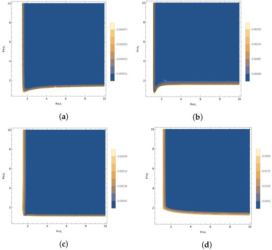
Fractalfract 09 00089 g003
Figure 4. The plots where the tenth approximant of (28) guarantees certain truncation error bounds for (26).
Fractalfract 09 00089 g004
Table 3. Relative error of fifth partial sum and fifth approximant.
z(23)(24)(25)
( 0.8 , 0.7 ) 1.1185 3.7401 × 10 1 1.0841 × 10 4
( 0.1 , 0.1 ) 0.1984 1.3790 × 10 9 1.7449 × 10 12
( 0.5 , 0.7 ) 0.3396 2.0795 × 10 3 1.4715 × 10 3
( 0.9 , 0.1 ) 0.6253 2.7472 × 10 2 1.3940 × 10 4
( 0.2 , 0.3 ) 0.4734 2.2374 × 10 5 1.7797 × 10 8
( 0.1 , 0.8 ) 0.7373 2.0631 × 10 2 3.5972 × 10 5
( 0.9 , 0.9 ) 1.2297 2.4591 2.8455 × 10 4
( 2 , 4 ) 1.7422 2.9054 × 10 + 5 2.3425 × 10 2
( 5 , 10 ) 1.9697 1.0147 × 10 + 9 0.3417 × 10 1
( 8 , 10 ) 2.0853 2.0193 × 10 + 5 0.9356 × 10 1
Table 4. Relative error of fifth partial sum and fifth approximant.
z(26)(27)(28)
( 0.6 , 0.6 ) 3.9023 1.1536 × 10 + 2 9.1384 × 10 1
( 0.9 , 0.8 ) 2.3654 8.0419 4.5692 × 10 2
( 1.5 , 1.4 ) 1.4675 5.5267 × 10 2 7.2177 × 10 4
( 2 , 3 ) 9.6031 × 10 1 1.1374 × 10 4 4.1428 × 10 5
( 10.9 ) 2.2125 × 10 1 5.8012 × 10 10 1.0153 × 10 11
( 20 , 40 ) 7.6553 × 10 1 7.1868 × 10 14 1.9746 × 10 15
( 50 , 70 ) 3.4585 × 10 2 8.8000 × 10 17 1.8847 × 10 19
( 100 , 110 ) 2.0099 × 10 2 7.8850 × 10 19 3.6751 × 10 22
( 500 , 1000 ) 3.0025 × 10 3 2.1889 × 10 26 1.6536 × 10 29
Disclaimer/Publisher’s Note: The statements, opinions and data contained in all publications are solely those of the individual author(s) and contributor(s) and not of MDPI and/or the editor(s). MDPI and/or the editor(s) disclaim responsibility for any injury to people or property resulting from any ideas, methods, instructions or products referred to in the content.

