Article

Probing Malware Propagation Model with Variable Infection Rates Under Integer, Fractional, and Fractal–Fractional Orders

1
Department of Mathematics, Quaid-i-Azam University, Islamabad 45320, Pakistan
2
Department of Mathematics and Statistics, Ripha International University, Haj Complex I-14, Islamabad 44000, Pakistan
3
Office of Research, Innovation and Commercialization, University of Management and Technology, Lahore 54770, Pakistan
4
Department of Mathematics, College of Science, King Saud University, Riyadh P.O. Box 2455, Saudi Arabia
5
Department of Computing, Mathematics and Electronics, “1 Decembrie 1918” University of Alba Iulia, 510009 Alba Iulia, Romania
6
Faculty of Mathematics and Computer Science, Transilvania University of Brasov, Iuliu Maniu Street 50, 500091 Brasov, Romania
*
Authors to whom correspondence should be addressed.
Fractal Fract. 2025, 9(2), 90; https://doi.org/10.3390/fractalfract9020090
Submission received: 12 December 2024 / Revised: 21 January 2025 / Accepted: 22 January 2025 / Published: 1 February 2025

Abstract

Malware software has become a pervasive threat in computer and mobile technology attacks. Attackers use this software to obtain information about users of the digital world to obtain benefits by hijacking their data. Antivirus software has been developed to prevent the propagation of malware, but this problem is not yet under control. To develop this software, we have to check the propagation of malware. In this paper, we explore an advanced malware propagation model with a time-delay factor and a variable infection rate. To better understand this model, we use fractal–fractional theory. We use an exponential decay kernel for this. For theoretical purposes (existence, uniqueness, and stability), we use the results from fixed-point theory, and, for numerical purposes, a Lagrange two-point interpolation polynomial is used to develop an algorithm. Matlab R2016a is used for simulation, and the physical significance is assessed. We examine the impact of different fractal and fractional orders for various parameters. Moreover, we compare four different mathematical models (classical, fractional, fractal, and fractal–fractional). Also, constant and variable fractional and fractal orders are compared using graphs. We investigate the idea that significant perturbation in infected nodes might be due to minor changes. This work may help with developing antivirus strategies in real life.

1. Introduction

Malware software, commonly known as malware, is used by cyber criminals. They use it to obtain information about individuals and their activities. They use it to track activities on the Internet and obtain sensitive information about accounts as well. Malware software has defense systems, which can be hidden from antivirus programs [1].
The most common form of malware is adware. In the present era, marketing is essential. Today, the Internet and smartphones are usually used for marketing. We see many advertisements when we use a mobile application or visit a website. There are many possibilities for adware attacks in such contexts. Cyber criminals can obtain information about whether or not they use an app [2]. Much work has been devoted to studying the behavior of malware, and many methods have been developed to protect individuals and computers from it. For example, machine learning processes have been used [2] for this purpose, and malware behavior has been compared using machine learning and deep learning techniques [3].
A general taxonomy of malware is presented in [4]. Malware belongs to different categories, such as the following viruses, viruses, trojans, spyware (adware, keylogger, trackware, cookie, riskware, sniffer), ransomware, scareware, diallerware, bots (spamware, reverse shell), rootkit (bootkit), backdoor, browser hijackers, and downloaders. Authors have also described malware concealment techniques such as encryption, packing, obfuscation, polymorphism, and metamorphism. Three methods of malware analysis—static, dynamic, and hybrid—can be used to detect it.
Malware propagation resembles transmitting infectious diseases in humans and other living bodies. It is a form of ’Mathematical Epidemiology’; the most commonly used model is the ‘Susceptible, Infected, and Recovered model’ (see [5] and the references therein). Much work has focused on classical calculus in this area. Now, researchers are working on fractional calculus. Fractional calculus is the generalization of the ordinary derivative and integral concepts [6,7,8].
The initially introduced Riemann–Liouville and Caputo fractional derivatives had some kernel difficulties. So, to overcome these difficulties, the Caputo and Fabrizio fractional derivative was introduced (2015), with the kernel in the form of an exponential function. Atangana and Baleanu replaced this the following year with the Mittag–Leffler function [9,10]. Over time, the new concept of “fractal” opened a vast field for researchers. The concepts of differentiation and integration were introduced [11] to solve differential equations using three kinds of kernels, i.e., power law, exponential decay, and Mittag–Leffler.
This has attracted many researchers in science, technology, engineering, etc. Significant work was conducted on mathematical modeling in the form of the fractal–fractional derivative [12]. Different models have been constructed for different diseases. Their solutions were found using concepts from pure mathematics [13,14,15,16,17] and fractal theory [18,19], along with numerical simulations with different kernels [20,21,22,23,24,25].
Motivated by the application of fractal–fractional theory in many diseases, we decided to treat malware propagation using the concept of fractal–fractional derivatives. We considered the malware propagation ’Susceptible, Infected and Removed’ model, as it is a basic model used in epidemiology. Investigating different malware propagation models, we decided to consider the model in [26]. The authors described this model as involving two main aspects: the variable infection rate and the time delay factor. These two variables capture real-world malware outbreaks’ irregular, nonlinear dynamics, such as their varying infection rates due to different network topologies, system vulnerabilities, or user behaviors. They aimed to develop an accurate model that can be used to predict malware propagation in computer networks. As fractional derivatives introduce a novel way to model these nonlinear, irregular, and scale-invariant behaviors, these derivatives enable a better representation of complex time-dependent processes.
Classical models often represent the propagation of malware in networked systems by assuming constant infection rates and immediate spread. However, in real-world networks, malware spread is influenced by factors such as varying infection rates, delays in propagation, and complex network topologies. This research introduces a novel modeling approach based on fractal–fractional derivatives, which accounts for the nonlinear, time-varying dynamics of malware propagation. The scientific problem is the lack of accurate and realistic models for malware propagation that can account for the complexity, variability, and delays in real-world scenarios. Our model addresses this gap using advanced mathematical techniques to understand these dynamics better and predict them.
Our goal was to investigate the behavior of this model under changes in fractal orders and fractional orders with an exponential decay kernel. We wanted to find a solution that can give us better estimates of the parameters to prevent malware propagation. We also wanted to explore its physical significance. This model is different because it involves a nonlinear function to represent an undetermined dynamical parameter that varies due to the sensitivity of the infection rate. We wanted to improve the accuracy of malware spread predictions, optimize security responses, and design more resilient defense strategies.
This paper is structured as follows: laying the groundwork of our research, Section 2 provides essential definitions and theorems. In Section 3, we present a classical mathematical model, and Section 4, we describe a fractal–fractional mathematical model. The model is converted into a fixed-point problem in Section 5. The existence, uniqueness, and stability of the solution are established in Section 6, Section 7 and Section 8. Section 9 constitutes a computational algorithm using a two-point Lagrangian interpolation formula due to its accuracy, convergence, and simplicity. MATLAB R2016a was used to implement the codes for arbitrary fractal and fractional orders and key parameters. Section 10 discusses the simulation results, and in Section 11, we conclude this paper.

2. Preliminaries

We represent some definitions and results from classical and fractional calculus used to develop the theory for our model.

2.1. Classical Calculus

We use the following results [13]:
Let Ψ represents a subclass of non-decreasing functions ψ : [ 0 , ) [ 0 , ) such that
j = 1 ψ j ( ϑ ) < ϑ > 0 ,
where ψ j is the jth iteration of ψ ; then, we have
Lemma 1 
([13]). Each function ψ : [ 0 , ) [ 0 , ) satisfies the following condition:
if ψ Ψ is non-decreasing, for each ϑ > 0 ,
lim j ψ j ( ϑ ) = 0 ψ ( ϑ ) < ϑ .
Definition 1 
([13]). Given a normed space X and function F : X X with ψ : [ 0 , ) [ 0 , ) and ϕ : X 2 [ 0 , ) , F is called a ϕ - ψ - c o n t r a c t i o n if for u 1 , u 2 X , ϕ ( u 1 , u 2 ) · d ( F u 1 , F u 2 ) ψ ( d ( u 1 , u 2 ) ) .
Definition 2 
([13]). If F : X X and ϕ : X 2 [ 0 , )   F is said to be ϕ - a d m i s s i b l e
if for u 1 , u 2 X ,   ϕ ( u 1 , u 2 ) 1 ϕ ( F u 1 , F u 2 ) 1 .
Using Definition 1 and Definition 2, the following theorem is established for the existence of a fixed point:
Theorem 1 
([13]). Given a complete metric space ( X , d ) and ϕ-ψ- c o n t r a c t i o n F , F : X X . F has a fixed point if the following conditions hold:
(i) 
F is ϕ- a d m i s s i b l e ;
(ii) 
x 0 X with the condition ϕ ( x 0 , F x 0 ) 1 ;
(iii) 
A sequence { x n } X , such that ϕ ( x n , x n + 1 ) 1 for all n and x n x X as n , implies ϕ ( x n , x ) 1 for all n N .
For the existence of a solution in support of Theorem 1, we define the Leray–Schauder criteria as follows:
Theorem 2 
([15]). Given a Banach space X , E X is a bounded, closed, and compact set in X . For an open set A such that 0 A E , a compact, continuous operator K : A ¯ E implies either K has a fixed point in A ¯ or ∃ x A and ϰ ( 0 , 1 ) such that x = ϰ G ( x ) .
The Arzela–Ascoli theorem is given below to prove compactness.
Theorem 3 
([16]). Let H R n , y C ( H , R m ) . Then, y is compact ; y is closed, bounded, and equicontinuous.

2.2. Fractal Calculus

Nowadays, fractal derivatives are employed to understand the behavior of variables. We examine the behavior of a variable with respect to a scaled variable [18,19].
Definition 3.
The fractal derivative of a function f ( ϑ ) with fractal order p is
d f ( ϑ ) d ϑ p = lim ϑ ϑ 1 f ( ϑ ) f ( ϑ 1 ) ϑ p ϑ 1 p ,
where p ( 0 , 1 ) .
Integrating the ideas of fractional and fractal derivatives, Atangana introduced a new concept of differentiation [11]:
Definition 4. 
Let G ( ϑ ) be continuous on ( a , b ) , and if G is fractally differentiable on this interval having order p , then the fractal–fractional derivative of G having order q in the Riemannliouville sense in terms of exponential decay kernel is defined as
D a , ϑ q , p F F E G ( ϑ ) = M ( q ) Γ ( 1 q ) d d ϑ p a ϑ e x p [ q 1 q ( ϑ w ) ] G ( w ) d w ,
where ( 0 < p , q n ) , n N and M ( 0 ) = M ( 1 ) = 1 .
With the same operator, the fractal–fractional integral associated with the fractal–fractional derivative is constructed with the exponential decay kernel defined above.
Definition 5. 
Let G ( ϑ ) be continuous on ( a , b ) . The fractal–fractional integral of G is
I a , ϑ q , p F F E G ( ϑ ) = p ( 1 q ) ϑ ( p 1 ) G ( ϑ ) M ( q ) + p q M ( q ) a ϑ w p 1 G ( w ) d w .

2.2.1. Variable-Order Fractional Derivative

As defined in [27], we define
Definition 6. 
Let G ( ϑ ) be continuous on ( a , b ) , and if G is fractal differentiable on this interval having order p , then the fractal-fractional derivative of G having variable-order q ( ϑ ) in the Riemann–Liouville sense in terms of the exponential decay kernel is defined as
D a , ϑ q ( ϑ ) , p F F E G ( ϑ ) = M ( q ( ϑ ) ) Γ ( 1 q ( ϑ ) ) d d ϑ p a ϑ e x p [ q ( ϑ ) 1 q ( ϑ ) ( ϑ u ) ] G ( u ) d u ,
where ( 0 < p , q ( ϑ ) 1 ) and M ( 0 ) = M ( 1 ) = 1 .
Definition 7. 
Let G ( ϑ ) be continuous on ( a , b ) , then the fractal–fractional integral of G ( ϑ ) with an exponential decay kernel having variable-order q ( ϑ ) is
I a , ϑ q ( ϑ ) , p F F E G ( ϑ ) = p ( 1 q ( ϑ ) ) ϑ ( p 1 ) G ( ϑ ) M ( q ( ϑ ) ) + p q ( ϑ ) M ( q ( ϑ ) ) a ϑ u p 1 G ( u ) d u .

2.2.2. Variable-Order Fractal Derivative

Najat et al. defined a Riemann–Liouville fractal fractional derivative with a variable fractal order [28].
Definition 8. 
Let G ( ϑ ) be a differential function. Let 0 < q 1 and p ( ϑ ) > 0 be a continuous function, then the fractional derivative fractal of G ( ϑ ) in the Riemann–Liouville sense in terms of the exponential decay kernel is defined as
D a , ϑ q , p ( ϑ ) F F E G ( ϑ ) = M ( q ) Γ ( 1 q ) d d ϑ p ( ϑ ) a ϑ e x p [ q 1 q ( ϑ u ) ] G ( u ) d u ,
where G ( ϑ ) has fractional order q and fractal dimension p ( ϑ ) , 0 < p ( ϑ ) , q 1 and M ( 0 ) = M ( 1 ) = 1 .
Definition 9. 
The fractal–fractional integral of G having order q and fractal variable dimension p ( ϑ ) in the Riemann–Liouville sense in terms of an exponential decay kernel with order q is
I a , ϑ q , p ( ϑ ) F F E G ( ϑ ) = p ( ϑ ) ( 1 q ) ϑ ( p ( ϑ ) 1 ) G ( ϑ ) M ( q ) + p ( ϑ ) q M ( q ) a ϑ u p ( ϑ ) 1 G ( u ) [ p ( u ) ln ( u ) + p ( u ) u ] u p ( u ) d u .

3. Description of Model

Now, we describe the mathematical model using ordinary differential equations. Feng et al. [26] presented a model of malware propagation on the Internet for the states known as susceptible, infected, and removed/recovered, with the assumption that the total number of nodes in the network at time ϑ is N ( ϑ ) . It was also assumed that all nodes change as time passes. In the model, the susceptible state indicates that a node can be easily exploited; the infected state mean that during the infected period, it remains infectious and can also infect its neighboring nodes; and the removed/recovered state means that an installed detection tool helps identify and remove malware or a node was installed with a software patch to eliminate node vulnerability to malware.
The symbols and meanings of the variables and parameters of the model (1) are given in the following Table 1.
Considering the definitions of the states in Feng et al. [26], we present the model as ordinary differential equations as
d Δ d ϑ = Π θ β 0 f ( ( ϑ ) ) Δ ( ϑ ) ( σ + ν ) Δ ( ϑ ) + ζ Θ ( ϑ τ ) , d d ϑ = β 0 f ( ( ϑ ) ) Δ ( ϑ ) ( σ + ρ ) ( ϑ ) , d Θ d ϑ = ( 1 Π ) θ + ν Δ ( ϑ ) + ρ ( ϑ ) ζ Θ ( ϑ τ ) σ Θ ( ϑ ) .
β ( ϑ ) is the infection rate, which depends on many factors discussed in this paper, so we defined β ( ϑ ) = β 0 f 1 ( ( ϑ ) ) , where f 1 is a nonlinear function of ℵ. Again, we assume f ( ( ϑ ) ) = f 1 ( ( ϑ ) ) ( ϑ ) , which is an undetermined dynamical operator. To determine this, the authors defined f ( ( ϑ ) ) = ( ϑ ) 1 + α ( ϑ ) , where α is used to adjust the sensitivity of the infection rate to the number of infected nodes ( ϑ ) [26].
Definition 10. 
The disease-free equilibrium ( D F E ) point for the model is
E = ( ( Π σ + ζ ) θ σ ( σ + ζ + ν ) , 0 , ( ( 1 Π ) σ + ν ) θ σ ( σ + ζ + ν ) ) .
Definition 11. 
Now, we find the threshold of the system.
Take disease class
d d ϑ = β 0 f ( ( ϑ ) ) Δ ( ϑ ) ( σ + ρ ) ( ϑ ) .
Assume
Z 1 ( ( ϑ ) ) = β 0 f ( ( ϑ ) ) Δ ( ϑ ) ,
and
Z 2 ( ( ϑ ) ) = ( σ + ρ ) ( ϑ ) ,
then,
Z 1 = d Z 1 d = β 0 f ( ( ϑ ) ) Δ ( ϑ )
and
Z 2 = d Z 2 d = ( σ + ρ ) .
Moreover,
1 Z 2 = 1 ( σ + ρ ) .
Evaluating Z 1 and 1 Z 2 at the disease-free equilibrium point, we obtain
Z 1 = β 0 f ( 0 ) ( Π σ + ζ ) θ σ ( σ + ζ + ν ) ,
and
1 Z 2 = 1 σ + ρ .
The threshold of the system is
R 0 = Z 1 · 1 Z 2
at point E.
Hence,
R 0 = β 0 θ ( Π σ + ζ ) f ( 0 ) σ ( σ + ρ ) ( σ + ζ + ν ) .

4. Fractal–Fractional Mathematical Model

Now, we convert model (1) in terms of fractal–fractional derivatives with exponential decay kernel:
D 0 , ϑ q , p F F E Δ ( ϑ ) = Π θ β 0 f ( ( ϑ ) ) Δ ( ϑ ) ( σ + ν ) Δ ( ϑ ) + ζ Θ ( ϑ τ ) , D 0 , ϑ q , p F F E ( ϑ ) = β 0 f ( ( ϑ ) ) Δ ( ϑ ) ( σ + ρ ) ( ϑ ) , D 0 , ϑ q , p F F E Θ ( ϑ ) = ( 1 Π ) θ + ν Δ ( ϑ ) + ρ ( ϑ ) ζ Θ ( ϑ τ ) σ Θ ( ϑ ) ,
with ( Δ ( 0 ) , ( 0 ) , Θ ( 0 ) ) = ( Δ 0 , 0 , Θ 0 ) 0 .
N ( ϑ ) = Δ ( ϑ ) + ( ϑ ) + Θ ( ϑ ) for ϑ I = [ 0 , T ] , where T > 0 and 0 < p , q 1 . All parameters take non-negative values.

5. Fractal–Fractional Model as a Fixed-Point Problem

Now, we convert mathematical model (2) to a fixed-point problem.
Consider a Banach space Ξ = Y 3 , where Y = C ( I , R ) represents the class of all continuous functions. We define the norm as
| | ϝ | | Ξ = | | ( Δ , , Θ ) | | Ξ = m a x { | Δ ( ϑ ) | + | ( ϑ ) | + | Θ ( ϑ ) | : ϑ I } .
Model 1 can be rewritten as
Υ 1 ( ϑ , Δ ( ϑ ) , ( ϑ ) , Θ ( ϑ ) ) = Π θ β 0 f ( ( ϑ ) ) Δ ( ϑ ) ( σ + ν ) Δ ( ϑ ) + ζ Θ ( ϑ τ ) , Υ 2 ( ϑ , Δ ( ϑ ) , ( ϑ ) , Θ ( ϑ ) ) = β 0 f ( ( ϑ ) ) Δ ( ϑ ) ( σ + ρ ) ( ϑ ) , Υ 3 ( ϑ , Δ ( ϑ ) , ( ϑ ) , Θ ( ϑ ) ) = ( 1 Π ) θ + ν Δ ( ϑ ) + ρ ( ϑ ) ζ Θ ( ϑ τ ) σ Θ ( ϑ ) .
Comparing models (1) and (3), we have
D 0 , ϑ q , p F F E Δ ( ϑ ) = Υ 1 ( ϑ , Δ ( ϑ ) , ( ϑ ) , Θ ( ϑ ) ) , D 0 , ϑ q , p F F E ( ϑ ) = Υ 2 ( ϑ , Δ ( ϑ ) , ( ϑ ) , Θ ( ϑ ) ) , D 0 , ϑ q , p F F E Θ ( ϑ ) = Υ 3 ( ϑ , Δ ( ϑ ) , ( ϑ ) , Θ ( ϑ ) ) .
Since
D a , ϑ q , p F F E g ( ϑ ) = M ( q ) Γ ( 1 q ) d d ϑ p a ϑ e x p [ q 1 q ( ϑ u ) ] g ( u ) d u
D a , ϑ q , p F F E g ( ϑ ) = M ( q ) Γ ( 1 q ) 1 p ϑ p 1 d d ϑ a ϑ e x p [ q 1 q ( ϑ u ) ] g ( u ) d u
D a , ϑ q , p F F E g ( ϑ ) = 1 p ϑ p 1 M ( q ) Γ ( 1 q ) d d ϑ a ϑ e x p [ q 1 q ( ϑ u ) ] g ( u ) d u
Now, we can write
M ( q ) Γ ( 1 q ) d d ϑ a ϑ e x p [ q 1 q ( ϑ u ) ] g ( u ) d u
as a Riemann–Liouville fractional derivative with an exponential decay kernel.
Therefore, we obtain
D 0 , ϑ q , p F F E g ( ϑ ) = ( 1 p ϑ p 1 ) R L D 0 , ϑ q g ( ϑ )
So, model (4) can be written as
( 1 p ϑ p 1 ) R L D 0 , ϑ q Δ ( ϑ ) = Υ 1 ( ϑ , Δ ( ϑ ) , ( ϑ ) , Θ ( ϑ ) ) , ( 1 p ϑ p 1 ) R L D 0 , ϑ q ( ϑ ) = Υ 2 ( ϑ , Δ ( ϑ ) , ( ϑ ) , Θ ( ϑ ) ) , ( 1 p ϑ p 1 ) R L D 0 , ϑ q Θ ( ϑ ) = Υ 3 ( ϑ , Δ ( ϑ ) , ( ϑ ) , Θ ( ϑ ) ) .
Hence, we have
D 0 , ϑ q R L Δ ( ϑ ) = p ϑ p 1 Υ 1 ( ϑ , Δ ( ϑ ) , ( ϑ ) , Θ ( ϑ ) ) , D 0 , ϑ q R L ( ϑ ) = p ϑ p 1 Υ 2 ( ϑ , Δ ( ϑ ) , ( ϑ ) , Θ ( ϑ ) ) , D 0 , ϑ q R L Θ ( ϑ ) = p ϑ p 1 Υ 3 ( ϑ , Δ ( ϑ ) , ( ϑ ) , Θ ( ϑ ) ) .
In general, model (6) can be written as
D 0 , ϑ q R L ϝ ( ϑ ) = p ϑ p 1 Υ ( ϑ , ϝ ( ϑ ) ) , ϝ ( 0 ) = ϝ 0 ,
where
( p , q ) ( 0 , 1 ] , ϑ I , ϝ ( ϑ ) = ( Δ ( ϑ ) , ( ϑ ) , Θ ( ϑ ) ) , ϝ 0 = ( Δ 0 , 0 , Θ 0 ) .
Using a fractal–fractional integral for model (7), we have
ϝ ( ϑ ) = ϝ ( 0 ) + p ( 1 q ) ϑ ( p 1 ) Υ ( ϑ , ϝ ( ϑ ) ) M ( q ) + p q M ( q ) 0 ϑ w p 1 Υ ( w , ϝ ( w ) ) d w ,
where M ( 0 ) = M ( 1 ) = 1 .
We can also write it as
Δ ( ϑ ) = Δ ( 0 ) + p ( 1 q ) ϑ ( p 1 ) Υ 1 ( ϑ , Δ ( ϑ ) , ( ϑ ) , Θ ( ϑ ) ) M ( q ) + p q M ( q ) 0 ϑ w p 1 Υ 1 ( w , ϝ ( w ) ) d w , ( ϑ ) = ( 0 ) + p ( 1 q ) ϑ ( p 1 ) Υ 2 ( ϑ , Δ ( ϑ ) , ( ϑ ) , Θ ( ϑ ) ) M ( q ) + p q M ( q ) 0 ϑ w p 1 Υ 2 ( w , ϝ ( w ) ) d w , Θ ( ϑ ) = Θ ( 0 ) + p ( 1 q ) ϑ ( p 1 ) Υ 3 ( ϑ , Δ ( ϑ ) , ( ϑ ) , Θ ( ϑ ) ) M ( q ) + p q M ( q ) 0 ϑ w p 1 Υ 3 ( w , ϝ ( w ) ) d w .
So, model (2) can be transformed into a fixed-point problem:
An operator F : Ξ Ξ is defined as
F ( ϝ ( ϑ ) ) = ϝ ( 0 ) + p ( 1 q ) ϑ ( p 1 ) Υ ( ϑ ) M ( q ) + p q M ( q ) 0 ϑ w p 1 Υ ( w , ϝ ( w ) ) d w .

6. Existence of Solution

For existence, we prove the following theorem based on Theorem 1 [24].
Theorem 4. 
Suppose that V : R 3 × R 3 R , ψ Ψ , and Υ C ( J × Ξ , Ξ ) satisfy the following three conditions:
( β 1 ): ϝ 1 , ϝ 2 Ξ and ϑ I ,
| Υ ( ϑ , ϝ 1 ( ϑ ) ) Υ ( ϑ , ϝ 2 ) ( ϑ ) | 1 ψ ( | ϝ 1 ( ϑ ) ϝ 2 ( ϑ ) | ) , with V ( ϝ 1 ( ϑ ) , ϝ 2 ( ϑ ) ) 0 and 1 = M ( q ) p ( 1 q ) ϑ p 1 + q ϑ p .
( β 2 ): ϝ 0 Ξ and ϑ I , V ( ϝ 0 ( ϑ ) , F ( ϝ 0 ( ϑ ) ) ) 0 and V ( ϝ 1 ( ϑ ) , ϝ 2 ( ϑ ) ) 0   V ( F ( ϝ 1 ( ϑ ) ) , F ( ϝ 2 ( ϑ ) ) ) 0 ;
( β 3 ): { ϝ n } n 1 Ξ with ϝ n ϝ ,   V ( ϝ n ( ϑ ) , ϝ n + 1 ( ϑ ) 0 V ( ϝ n ( ϑ ) ) , ϝ ( ϑ ) ) 0 , for every n, ϑ I .
Then, we say that F has a fixed point, and a solution of the FF model exists.
Proof. 
Take ϝ 1 , ϝ 2 Ξ so that
V ( ϝ 1 ( ϑ ) , ϝ 2 ( ϑ ) ) 0 ,
for each ϑ I .
Consider
| F ( ϝ 1 ( ϑ ) ) F ( ϝ 2 ( ϑ ) ) | = | p ( 1 q ) ϑ p 1 [ Υ ( w , ϝ 1 ( w ) ) Υ ( w , ϝ 2 ( w ) ) ] M ( q ) + p q M ( q ) 0 ϑ w ( p 1 ) [ Υ ( w , ϝ 1 ( w ) ) Υ ( w , ϝ 2 ( w ) ) ] d w |
| F ( ϝ 1 ( ϑ ) ) F ( ϝ 2 ( ϑ ) ) | p ( 1 q ) ϑ p 1 | Υ ( w , ϝ 1 ( w ) ) Υ ( w , ϝ 2 ( w ) ) | M ( q ) + p q M ( q ) 0 ϑ w ( p 1 ) | Υ ( w , ϝ 1 ( w ) ) Υ ( w , ϝ 2 ( w ) ) | d w
Utilizing ( β 1 ) , we deduce
| F ( ϝ 1 ( ϑ ) ) F ( ϝ 2 ( ϑ ) ) | p ( 1 q ) ϑ p 1 M ( q ) 1 ψ ( | ϝ 1 ( w ) ϝ 2 ( w ) | ) + p q M ( q ) 0 ϑ w ( p 1 ) 1 ψ ( | ϝ 1 ( w ) ϝ 2 ( w ) | ) d w
Now, applying the definition of the norm,
| F ( ϝ 1 ( ϑ ) ) F ( ϝ 2 ( ϑ ) ) | p ( 1 q ) ϑ p 1 M ( q ) 1 ψ ( | | ϝ 1 ϝ 2 | | Ξ ) + p q M ( q ) 0 ϑ w ( p 1 ) 1 ψ ( | | ϝ 1 ϝ 2 | | Ξ ) d w
After simplification using the beta function and value of 1 , we have
| F ( ϝ 1 ( ϑ ) ) F ( ϝ 2 ( ϑ ) ) | ψ ( | | ϝ 1 ϝ 2 | | Ξ ) .
We can write this as
d ( F ( ϝ 1 ) , F ( ϝ 2 ) ) ψ ( d ( ϝ 1 , ϝ 2 ) ) .
Furthermore, we define ϕ : Ξ 2 [ 0 , ) with the condition
ϕ ( ϝ 1 , ϝ 2 ) = 1 for V ( ϝ 1 ( ϑ ) , ϝ 2 ( ϑ ) ) 0 , which is zero otherwise;
then, for each ϝ 1 , ϝ 2 Ξ , we can write Equation (12) as
ϕ ( ϝ 1 , ϝ 2 ) d ( F ( ϝ 1 ) , F ( ϝ 2 ) ) ψ ( d ( ϝ 1 , ϝ 2 ) ) .
Equation (13) implies that F is a ϕ - ψ - c o n t r a c t i o n .
Now, we assume that ϝ 1 , ϝ 2 Ξ , such that ϕ ( ϝ 1 , ϝ 2 ) 1 .
This implies
V ( ϝ 1 ( ϑ ) , ϝ 2 ( ϑ ) ) 0 ,
and ( β 2 )
V ( ϝ 0 ( ϑ ) , F ( ϝ 0 ( ϑ ) ) ) 0 and V ( ϝ 1 ( ϑ ) , ϝ 2 ( ϑ ) ) 0   V ( F ( ϝ 1 ( ϑ ) ) , F ( ϝ 2 ( ϑ ) ) ) 0 .
Now applying ϕ , we have
ϕ ( F ( ϝ 1 ) , F ( ϝ 2 ) ) 1 .
This implies F is ϕ - a d m i s s i b l e . (*)
Also, from ( β 2 ), we see that for some ϝ 0 in Ξ , ϑ I , V ( ϝ 0 ( ϑ ) , F ( ϝ 0 ( ϑ ) ) ) 0 implies ϕ ( ϝ 0 , F ( ϝ 0 ) ) 1 . (**)
Next, we take { ϝ n } n 1 Ξ such that ϝ n ϝ as n and ϕ ( ϝ n , ϝ n + 1 ) 1 for all n.
Applying the definition of ϕ , we obtain V ( ϝ n ( ϑ ) , ϝ n + 1 ( ϑ ) ) 0 , and ( β 3 ) implies V ( ϝ n ( ϑ ) , ϝ ( ϑ ) ) 0 .
Hence, ϕ ( ϝ n , ϝ ) 1 for all n. (***)
The statements (*), (**), and (***), satisfy the conditions of Theorem 1. Hence, F has a fixed point. Thus, ϝ * is a solution of the ff model. □
Now, we define the following theorem based on Theorem 2 to establish the existence of the solution to the ff model.
Theorem 5. 
Let Ξ be a Banach space, N ϵ be a bounded and closed set in Ξ, and A be an open set in N ϵ with 0 A . Then, there exists a compact, continuous operator F from A ¯ N ϵ with conditions ( β 4 ) and ( β 5 ), which satisfies one of the two conditions:
(a) G has a fixed point in A ¯ ,
or
(b) there exist ϝ A and ω ( 0 , 1 ) such that ϝ = ω F ( ϝ ) ,
where
( β 4 ): suppose Υ C ( J × Ξ , Ξ ) , and there exist ϕ L 1 ( I , [ 0 , ) ) and B C ( [ 0 , ) , [ 0 , ) ) , where B is an increasing function satisfying condition | F ( ϑ , ϝ ( ϑ ) ) | ϕ ( ϑ ) B ( | ϝ ( ϑ ) | ) ϑ I and ϝ Ξ ;
( β 5 ): Ii ϕ * = s u p ϑ I | ϕ ( ϑ ) | , then a number s such that s ϝ 0 + λ 1 ϕ * B ( s ) > 1 , where λ 1 = p ( 1 q ) ϑ p 1 + q ϑ p M ( q ) .
Then, a solution to our model exists, provided that the conditions above are satisfied.
Proof. 
Take F : Ξ Ξ as
F ( ϝ ( ϑ ) ) = ϝ ( 0 ) + p ( 1 q ) ϑ ( p 1 ) Υ ( ϑ , ϝ ( ϑ ) ) M ( q ) + p q M ( q ) 0 ϑ w p 1 Υ ( w , ϝ ( w ) ) d w ,
and N ϵ = { ϝ Ξ : | | ϝ | | Ξ ϵ } for some positive ϵ .
To show that F is compact on N ϵ , we prove that F is uniformly bounded and equicontinuous.
Since Υ is continuous, this implies F is continuous.
Now, for ϝ in N ϵ , we have
| F ( ϝ ( ϑ ) ) | | ϝ ( 0 ) | + p ( 1 q ) ϑ ( p 1 ) | Υ ( ϑ , ϝ ( ϑ ) ) | M ( q ) + p q M ( q ) 0 ϑ w p 1 | Υ ( w , ϝ ( w ) ) | d w
Using ( β 4 ), we have
| F ( ϝ ( ϑ ) ) | ϝ 0 + p ( 1 q ) ϑ ( p 1 ) ϕ ( ϑ ) B ( | ϝ ( ϑ ) | ) M ( q ) + p q M ( q ) 0 ϑ w p 1 ϕ ( w ) B ( | ϝ ( w ) | ) d w ϝ 0 + p ( 1 q ) ϑ ( p 1 ) ϕ * B ( | | ϝ | | Ξ ) M ( q ) + p q M ( q ) 0 ϑ w p 1 ϕ * B ( | | ϝ | | Ξ ) d w ϝ 0 + ϕ * B ( | | ϝ | | Ξ ) [ p ( 1 q ) ϑ ( p 1 ) M ( q ) + p q M ( q ) 0 ϑ w p 1 d w ] ,
After simplification of the integral and applying the value of λ 1 , we obtain
| F ( ϝ ( ϑ ) ) | ϝ 0 + λ 1 ϕ * B ( ϵ )
Now, applying the norm, we obtain the following:
| | F ( ϝ ( ϑ ) ) | | ϝ 0 + λ 1 ϕ * B ( ϵ ) < .
This shows that F is uniformly bounded.
Now, for ϑ , ϑ 1 I such that ϑ < ϑ 1 and ϝ N ϵ arbitrarily. If we take Υ * = s u p | Υ ( ϑ , ϝ ( ϑ ) ) | , then
| F ( ϝ ( ϑ 1 ) ) F ( ϝ ( ϑ ) ) | = | p ( 1 q ) ϑ 1 ( p 1 ) Υ ( ϑ 1 , ϝ ( ϑ 1 ) ) M ( q ) + p q M ( q ) 0 ϑ 1 w ( p 1 ) Υ ( w , ϝ ( w ) ) d w p ( 1 q ) ϑ ( p 1 ) Υ ( ϑ , ϝ ( ϑ ) ) M ( q ) p q M ( q ) 0 ϑ w ( p 1 ) Υ ( w , ϝ ( w ) ) d w | | p ( 1 q ) [ ϑ 1 ( p 1 ) Υ ( ϑ 1 , ϝ ( ϑ 1 ) ϑ ( p 1 ) Υ ( ϑ , ϝ ( ϑ ) ) ] M ( q ) | + p q M ( q ) | 0 ϑ 1 w ( p 1 ) d w 0 ϑ w ( p 1 ) d w | · | Υ ( w , ϝ ( w ) | p ( 1 q ) [ ϑ 1 ( p 1 ) ϑ ( p 1 ) ] G * M ( q ) + p q M ( q ) [ ϑ 1 p ϑ p ] Υ * [ p ( 1 q ) + p q M ( q ) ] [ ϑ 1 p ϑ p ] Υ * .
Now, ϑ 1 ϑ implies | | F ( ϝ ( ϑ 1 ) ) F ( ϝ ( ϑ ) ) | | Ξ 0 .
This proves that F is equicontinuous. Hence, it is proved that F is compact.
As F satisfies the basic conditions of Theorem 5, it satisfies one. For this purpose, using ( β 5 ), we construct A = { ϝ Ξ : | | ϝ | | Ξ < s } , where s > 0 is defined above. Hence, we can write
| | F ( ϝ ( ϑ ) ) | | ϝ 0 + λ 1 ϕ * B ( s ) .
Assume ϝ A and η ( 0 , 1 ) , where ϝ = η F ( ϝ ) . For ϝ and η , we have
s = | | ϝ | | Ξ = η | | F ( ϝ ) | | Ξ < | | F ( ϝ ) | | Ξ < ϝ 0 + λ 1 ϕ * B ( | | ϝ | | Ξ ) < ϝ 0 + λ 1 ϕ * B ( s ) < s
which is impossible. So, we can say that the first condition F possesses a fixed point in A ¯ . □

7. Uniqueness

In this section, we prove uniqueness with the theorems using the Lipschitz condition.
Theorem 6. 
Let Δ , , Θ , Δ 1 , 1 , Θ 1 Y = C ( I , R ) and we suppose that
( Condition 1 ) : | | Δ | | σ 1 , | | | | σ 2 , α [ 0 , ) ,
then | | f ( ( ϑ ) ) | | = | | ( ϑ ) 1 + α ( ϑ ) | | | | ( ϑ ) | | | | 1 + α ( ϑ ) | | σ 3 (where σ 3 [ 0 , σ 2 ] ) ,
| | Θ | | σ 4 for some σ i > 0 , i = 1 , 2 , 3 , 4 .
Moreover, | | 1 1 + α ( ϑ ) | | b 1 , | | 1 1 + α 1 ( ϑ ) | | b 2 where b i = 1 α | | j ( ϑ ) | | , j = 1 , 2 and b = b 1 · b 2 , then Υ 1 , Υ 2 , Υ 3 are Lipschitz functions with values:
w 1 = ( β 0 σ 3 + σ + ν ) , w 2 = ( β 0 σ 1 b + σ + γ ) , w 3 = ( ζ + σ ) , where w i ( 0 , 1 ) , i = 1 , 2 , 3 .
Proof. 
Consider Υ 1 for each Δ , Δ 1 Y ; then, we have
| | Υ 1 ( ϑ , Δ ( ϑ ) , ( ϑ ) , Θ ( ϑ ) ) Υ 1 ( ϑ , Δ 1 ( ϑ ) , ( ϑ ) , Θ ( ϑ ) ) | | = | | ( Π θ β 0 f ( ( ϑ ) ) Δ ( ϑ ) ( σ + ν ) Δ ( ϑ ) + ζ Θ ( ϑ τ ) ) ( Π θ β 0 f ( ( ϑ ) ) Δ 1 ( ϑ ) ( σ + ν ) Δ 1 ( ϑ ) + ζ Θ ( ϑ τ ) ) | | = | | β 0 f ( ( ϑ ) ) ( Δ ( ϑ ) Δ 1 ( ϑ ) ) ( σ + ν ) ( Δ ( ϑ ) Δ 1 ( ϑ ) ) | | = | | ( β 0 f ( ( ϑ ) ) ( σ + ν ) ) ( Δ ( ϑ ) Δ 1 ( ϑ ) ) | | = | | ( ( β 0 f ( ( ϑ ) ) + ( σ + ν ) ) ) ( Δ ( ϑ ) Δ 1 ( ϑ ) ) | | = | | ( β 0 f ( ( ϑ ) ) + ( σ + ν ) ) ( Δ ( ϑ ) Δ 1 ( ϑ ) ) | | ( | | ( β 0 f ( ( ϑ ) ) + ( σ + ν ) ) | | ) | | Δ ( ϑ ) Δ 1 ( ϑ ) | | ( | | ( β 0 f ( ( ϑ ) ) | | + | | ( σ + ν ) | | ) | | Δ ( ϑ ) Δ 1 ( ϑ ) | | ( β 0 σ 3 + σ + ν ) | | Δ ( ϑ ) Δ 1 ( ϑ ) | | w 1 | | Δ ( ϑ ) Δ 1 ( ϑ ) | | .
Hence, Υ 1 is Lipschitz with respect to Δ with w 1 > 0 .
Taking Υ 2 for each , 1 Y , we have
| | Υ 2 ( ϑ , Δ ( ϑ ) , ( ϑ ) , Θ ( ϑ ) ) Υ 2 ( ϑ , Δ ( ϑ ) , 1 ( ϑ ) , Θ ( ϑ ) ) | | = | | ( β 0 f ( ( ϑ ) ) Δ ( ϑ ) ( σ + γ ) ( ϑ ) ) ( β 0 f ( 1 ( ϑ ) ) Δ ( ϑ ) ( σ + γ ) 1 ( ϑ ) ) | | = | | ( β 0 Δ ( ϑ ) ( f ( ( ϑ ) ) f ( 1 ( ϑ ) ) ) + ( σ + γ ) ( ( ϑ ) + 1 ( ϑ ) ) | | | | ( β 0 Δ ( ϑ ) ( f ( ( ϑ ) ) f ( 1 ( ϑ ) ) ) | | + | | ( σ + γ ) ( ( ϑ ) + 1 ( ϑ ) ) | | | β 0 | | | Δ ( ϑ ) | | | | ( f ( ( ϑ ) ) f ( 1 ( ϑ ) ) ) | | + | ( σ + γ ) | | | ( ( ϑ ) 1 ( ϑ ) ) | | β 0 σ 1 | | ( ϑ ) 1 + α ( ϑ ) 1 ( ϑ ) 1 + α 1 ( ϑ ) | | + ( σ + γ ) | | ( ϑ ) 1 ( ϑ ) ) | | β 0 σ 1 | | ( ϑ ) 1 ( ϑ ) | | 1 | | ( 1 + α ( ϑ ) ) ( 1 + α 1 ( ϑ ) ) | | + ( σ + γ ) | | ( ϑ ) 1 ( ϑ ) | | β 0 σ 1 b | | ( ϑ ) 1 ( ϑ ) | | + ( σ + γ ) | | ( ϑ ) 1 ( ϑ ) | | ( β 0 σ 1 b + σ + γ ) | | ( ϑ ) 1 ( ϑ ) | | w 2 | | ( ϑ ) 1 ( ϑ ) | | .
Hence, Υ 2 is Lipschitz with respect to ℵ with w 2 > 0 .
Considering Υ 3 for each Θ , Θ 1 Y , we take
| | Υ 3 ( ϑ , Δ ( ϑ ) , ( ϑ ) , Θ ( ϑ ) ) Υ 3 ( ϑ , Δ ( ϑ ) , ( ϑ ) , Θ 1 ( ϑ ) ) | | = | | ( ( 1 Π ) θ + ν Δ ( ϑ ) + ρ ( ϑ ) ζ Θ ( ϑ τ ) σ Θ ( ϑ ) ) ( ( 1 Π ) θ + ν Δ ( ϑ ) + ρ ( ϑ ) ζ Θ 1 ( ϑ τ ) σ Θ 1 ( ϑ ) ) | | = | | ζ ( Θ 1 ( ϑ τ ) Θ ( ϑ τ ) ) + σ ( Θ 1 ( ϑ ) Θ ( ϑ ) ) | | | | ζ ( Θ 1 ( ϑ τ ) Θ ( ϑ τ ) ) | | + | | σ ( Θ 1 ( ϑ ) Θ ( ϑ ) ) | | | ζ | | | Θ ( ϑ τ ) Θ 1 ( ϑ τ ) | | + | σ | | | ( Θ ( ϑ ) Θ 1 ( ϑ ) ) | | For ϑ I and for τ 0 , if ( ϑ τ ) I , taking ϑ * = m a x ( ϑ , ϑ τ ) , we have ζ | | Θ ( ϑ * ) Θ 1 ( ϑ * ) | | + σ | | Θ ( ϑ * ) Θ 1 ( ϑ * ) | | ( ζ + σ ) | | Θ ( ϑ * ) Θ 1 ( ϑ * ) | | w 3 | | Θ ( ϑ * ) Θ 1 ( ϑ * ) | | .
Hence, Υ 3 is Lipschitz with respect to Θ with w 3 > 0 . □
Using Theorem 6, we prove Theorem 7 to examine the uniqueness of the solution.
Theorem 7.
If | | Δ | | σ 1 , | | | | σ 2 , | | Θ | | σ 4 for some σ i > 0 , i = 1 , 2 , 3 , 4 and
w 1 = ( β 0 σ 3 + σ + ν ) , w 2 = ( β 0 σ 1 b + σ + γ ) , w 3 = ( ζ + σ ) , where 0 < w j < 1 , j = 1 , 2 , 3 ; then, the ff model has a unique solution if λ 1 w j < 1 for j = 1 , 2 , 3 .
Proof. 
Suppose there exist two solutions, ( Δ ( ϑ ) , ( ϑ ) , Θ ( ϑ ) ) and ( Δ * ( ϑ ) , * ( ϑ ) , Θ * ( ϑ ) ) , concerning condition 1 for the ff model. Then, we can write
Δ ( ϑ ) = Δ ( 0 ) + p ( 1 q ) ϑ ( p 1 ) Υ 1 ( ϑ , ϝ ( ϑ ) ) M ( q ) + p q M ( q ) 0 ϑ w p 1 Υ 1 ( w , ϝ ( w ) ) d w , Δ * ( ϑ ) = Δ ( 0 ) + p ( 1 q ) ϑ ( p 1 ) Υ 1 ( ϑ , ϝ * ( ϑ ) ) M ( q ) + p q M ( q ) 0 ϑ w p 1 Υ 1 ( w , ϝ * ( w ) ) d w .
Take
| | Δ ( ϑ ) Δ * ( ϑ ) | | = | | p ( 1 q ) ϑ ( p 1 ) [ Υ 1 ( ϑ , ϝ ( ϑ ) ) Υ 1 ( ϑ , ϝ * ( ϑ ) ) ] M ( q ) + p q M ( q ) 0 ϑ w ( p 1 ) ( Υ 1 ( w , ϝ ( w ) ) Υ 1 ( w , ϝ * ( w ) ) ) d w | | p ( 1 q ) ϑ ( p 1 ) | | Υ 1 ( ϑ , ϝ ( ϑ ) ) Υ 1 ( ϑ , ϝ * ( ϑ ) ) | | M ( q ) + p q M ( q ) 0 ϑ w ( p 1 ) | | Υ 1 ( w , ϝ ( w ) ) Υ 1 ( w , ϝ * ( w ) ) | | d w .
Since Υ 1 is taken with respect to Δ and Δ * , after integration and simplification,
| | Δ ( ϑ ) Δ * ( ϑ ) | | p ( 1 q ) ϑ p 1 + ϑ p q M ( q ) | | Υ 1 ( Δ ) Υ 1 ( Δ * ) | | .
Hence, using the previous results,
| | Δ ( ϑ ) Δ * ( ϑ ) | | λ 1 w 1 | | Δ ( ϑ ) Δ * ( ϑ ) | |
( 1 λ 1 w 1 ) | | Δ ( ϑ ) Δ * ( ϑ ) | | 0 .
As λ 1 w 1 < 1 , which is possible when | | Δ ( ϑ ) Δ * ( ϑ ) | | = 0 . Thus, Δ ( ϑ ) = Δ * ( ϑ ) .
Similarly, we take
( ϑ ) = ( 0 ) + p ( 1 q ) ϑ ( p 1 ) Υ 2 ( ϑ , ϝ ( ϑ ) ) M ( q ) + p q M ( q ) 0 ϑ w p 1 Υ 2 ( w , ϝ ( w ) ) d w , * ( ϑ ) = ( 0 ) + p ( 1 q ) ϑ ( p 1 ) Υ 2 ( ϑ , ϝ * ( ϑ ) ) M ( q ) + p q M ( q ) 0 ϑ w p 1 Υ 2 ( w , ϝ * ( w ) ) d w .
| | ( ϑ ) * ( ϑ ) | | = | | p ( 1 q ) ϑ ( p 1 ) [ Υ 2 ( ϑ , ϝ ( ϑ ) ) Υ 2 ( ϑ , ϝ * ( ϑ ) ) ] M ( q ) + p q M ( q ) 0 ϑ w ( p 1 ) ( Υ 2 ( w , ϝ ( w ) ) Υ 2 ( w , ϝ * ( w ) ) ) d w | | p ( 1 q ) ϑ ( p 1 ) | | Υ 2 ( ϑ , ϝ ( ϑ ) ) Υ 2 ( ϑ , ϝ * ( ϑ ) ) | | M ( q ) + p q M ( q ) 0 ϑ w ( p 1 ) | | Υ 2 ( w , ϝ ( w ) ) Υ 2 ( w , ϝ * ( w ) ) | | d w ,
as Υ 2 is related to and * . So, after integration and simplification, we have
| | ( ϑ ) * ( ϑ ) | | p ( 1 q ) ϑ p 1 + ϑ p q M ( q ) | | Υ 2 ( ) Υ 2 ( * ) | | .
Hence, we obtain
| | ( ϑ ) * ( ϑ ) | | λ 1 w 2 | | ( ϑ ) * ( ϑ ) | |
( 1 λ 1 w 2 ) | | ( ϑ ) * ( ϑ ) | | 0 .
As λ 1 w 2 < 1 , the above condition holds when | | ( ϑ ) * ( ϑ ) | | = 0 . This implies that ( ϑ ) = * ( ϑ ) .
Similarly, consider
Θ ( ϑ ) = Θ ( 0 ) + p ( 1 q ) ϑ ( p 1 ) Υ 3 ( ϑ , ϝ ( ϑ ) ) M ( q ) + p q M ( q ) 0 ϑ w p 1 Υ 3 ( w , ϝ ( w ) ) d w , Θ * ( ϑ ) = Θ ( 0 ) + p ( 1 q ) ϑ ( p 1 ) Υ 3 ( ϑ , ϝ * ( ϑ ) ) M ( q ) + p q M ( q ) 0 ϑ w p 1 Υ 3 ( w , ϝ * ( w ) ) d w .
Take
| | Θ ( ϑ ) Θ * ( ϑ ) | | = | | p ( 1 q ) ϑ ( p 1 ) [ Υ 3 ( ϑ , ϝ ( ϑ ) ) Υ 3 ( ϑ , ϝ * ( ϑ ) ) ] M ( q ) + p q M ( q ) 0 ϑ w ( p 1 ) ( Υ 3 ( w , ϝ ( w ) ) Υ 3 ( w , ϝ * ( w ) ) ) d w | | p ( 1 q ) ϑ ( p 1 ) | | Υ 3 ( ϑ , ϝ ( ϑ ) ) Υ 3 ( ϑ , ϝ * ( ϑ ) ) | | M ( q ) + p q M ( q ) 0 ϑ w ( p 1 ) | | Υ 3 ( w , ϝ ( w ) ) Υ 3 ( w , ϝ * ( w ) ) | | d w ,
since Υ 3 is taken with respect to Θ and Θ * . After integration and simplification, we have
| | Θ ( ϑ ) Θ * ( ϑ ) | | p ( 1 q ) ϑ p 1 + ϑ p q M ( q ) | | Υ 3 ( Θ ) Υ 3 ( Θ * ) | | .
By using the previous results,
| | Θ ( ϑ ) Θ * ( ϑ ) | | λ 1 w 3 | | Θ ( ϑ ) Θ * ( ϑ ) | |
( 1 λ 1 w 3 ) | | Θ ( ϑ ) Θ * ( ϑ ) | | 0 .
As λ 1 w 3 < 1 , the possibility is | | Θ ( ϑ ) Θ * ( ϑ ) | | = 0 . Thus, Θ ( ϑ ) = Θ * ( ϑ ) . That is, ( Δ ( ϑ ) , ( ϑ ) , Θ ( ϑ ) ) = ( Δ * ( ϑ ) , * ( ϑ ) , Θ * ( ϑ ) ) . Hence, the solution is unique. □

8. Stability

In this section, we check the stability of the solution using the Ulam–Hyers and Ulam–Hayers–Rassias theorems. First, we define the theorems for our model, definitions, and remarks; then, we prove them.
Definition 12. 
Model (4) is Ulam–Hyers-stable as in [29] if, for all ϵ i > 0 , there exists M i > 0 [ 0 , ) , depending upon Υ i , where i = 1 , 2 , 3 and, for all ϝ * , the condition is satisfied:
| F F E D 0 , ϑ q , p Δ * ( ϑ ) Υ 1 ( ϑ , ϝ * ( ϑ ) ) | ϵ 1 , | F F E D 0 , ϑ q , p * ( ϑ ) Υ 2 ( ϑ , ϝ * ( ϑ ) ) | ϵ 2 , | F F E D 0 , ϑ q , p Θ * ( ϑ ) Υ 3 ( ϑ , ϝ * ( ϑ ) ) | ϵ 3 .
Then, there exists ϝ Ξ , satisfying model (4) with another condition given below:
| Δ * ( ϑ ) Δ ( ϑ ) | M 1 ϵ 1 , | * ( ϑ ) ( ϑ ) | M 2 ϵ 2 , | Θ * ( ϑ ) Θ ( ϑ ) | M 3 ϵ 3 .
Remark 1. 
ϝ * Ξ is a solution if η i C ( [ 0 , T ] , [ 0 , ) ) such that for each ϑ I ,
(i) 
| η i ( ϑ ) | < ϵ i ,
(ii) 
D 0 , ϑ q , p F F E Δ * ( ϑ ) = Υ 1 ( ϑ , ϝ * ( ϑ ) ) + η 1 ( ϑ ) , D 0 , ϑ q , p F F E * ( ϑ ) = Υ 2 ( ϑ , ϝ * ( ϑ ) ) + η 2 ( ϑ ) , D 0 , ϑ q , p F F E Θ * ( ϑ ) = Υ 3 ( ϑ , ϝ * ( ϑ ) ) + η 3 ( ϑ ) .
Theorem 8. 
The ff model (4) is Ulam–Hayers-stable on I such that λ 1 w i < 1 , where w i and λ 1 are defined with the conditions as above.
Proof. 
Let ϵ 1 > 0 and Δ * Y such that
| F F E D 0 , ϑ q , p Δ * ( ϑ ) Υ 1 ( ϑ , ϝ * ( ϑ ) ) | ϵ 1 ,
From remark 1, we have
Δ * ( ϑ ) = Δ ( 0 ) + p ( 1 q ) ϑ p 1 Υ 1 ( ϑ , ϝ * ( ϑ ) ) M ( q ) + p q M ( q ) 0 ϑ w ( p 1 ) Υ 1 ( w , ϝ * ( w ) ) d w + p q M ( q ) 0 ϑ w ( p 1 ) η 1 ( w ) d w .
As Δ Y is unique, then
Δ ( ϑ ) = Δ ( 0 ) + p ( 1 q ) ϑ ( p 1 ) Υ 1 ( ϑ , ϝ ( ϑ ) ) M ( q ) + p q M ( q ) 0 ϑ w p 1 Υ 1 ( w , ϝ ( w ) ) d w .
That is,
| Δ * ( ϑ ) Δ ( ϑ ) | = | p ( 1 q ) ϑ ( p 1 ) [ Υ 1 ( ϑ , ϝ ( ϑ ) ) Υ 1 ( ϑ , ϝ ( ϑ ) ) ] M ( q ) + p q M ( q ) 0 ϑ w ( p 1 ) η 1 ( w ) d w + p q M ( q ) 0 ϑ w ( p 1 ) [ Υ 1 ( w , ϝ * ( w ) ) Υ 1 ( w , ϝ ( w ) ) ] d w | p ( 1 q ) ϑ ( p 1 ) | | Υ 1 ( ϑ , ϝ ( ϑ ) ) Υ 1 ( ϑ , ϝ ( ϑ ) ) | | M ( q ) + p q M ( q ) 0 ϑ u ( p 1 ) | η 1 ( w ) | d w + p q M ( q ) 0 ϑ w ( p 1 ) | | Υ 1 ( w , ϝ ( w ) ) Υ 1 ( w , ϝ * ( w ) ) | | d w p ( 1 q ) ϑ ( p 1 ) w 1 | | Δ * Δ | | M ( q ) + q ϑ p M ( q ) | η 1 | + p q M ( q ) 0 ϑ w ( p 1 ) w 1 | | Δ * Δ | | d w [ p ( 1 q ) ϑ ( p 1 ) + q ϑ p M ( q ) ] w 1 | | Δ * Δ | | + q ϑ p ϵ 1 M ( q ) λ 1 w 1 | | Δ * Δ | | + q ϑ p ϵ 1 M ( q ) .
Hence, we have
| | Δ * Δ | | λ 1 w 1 | | Δ * Δ | | + q ϑ p ϵ 1 M ( q ) ( 1 λ 1 w 1 ) | | Δ * Δ | | q ϑ p ϵ 1 M ( q ) | | Δ * Δ | | q ϑ p ϵ 1 M ( q ) ( 1 λ 1 w 1 ) .
If q ϑ p M ( q ) ( 1 λ 1 w 1 ) = M 1 , then | | Δ * Δ | | M 1 ϵ 1 .
Similarly, it is possible to prove that | | * | | M 2 ϵ 2 , and | | Θ * Θ | | M 3 ϵ 3 .
Thus, the ff model satisfies the Ulam−Hayers stability criteria. □
Definition 13 
([17]). Model (4) is Ulam–Hyers−Rassias-stable with respect to function ψ i , if, for all ϵ i > 0 , there exists M i > 0 [ 0 , ) , depending upon Υ i a n d ψ i , i = 1 , 2 , 3 and ∀ ϝ * satisfies the following condition:
| F F E D 0 , ϑ q , p Δ * ( ϑ ) Υ 1 ( ϑ , ϝ * ( ϑ ) ) | ϵ 1 ψ 1 ( ϑ ) , | F F E D 0 , ϑ q , p * ( ϑ ) Υ 2 ( ϑ , ϝ * ( ϑ ) ) | ϵ 2 ψ 2 ( ϑ ) , | F F E D 0 , ϑ q , p Θ * ( ϑ ) Υ 3 ( ϑ , ϝ * ( ϑ ) ) | ϵ 3 ψ 3 ( ϑ ) ,
there exists ϝ Ξ , satisfying the model with another condition given below:
| Δ * ( ϑ ) Δ ( ϑ ) | M 1 ϵ 1 ψ 1 ( ϑ ) , | * ( ϑ ) ( ϑ ) | M 2 ϵ 2 ψ 2 ( ϑ ) , | Θ * ( ϑ ) Θ ( ϑ ) | M 3 ϵ 3 ψ 3 ( ϑ ) .
Remark 2. 
ϝ * Ξ is a solution if η i C ( [ 0 , T ] , [ 0 , ) ) such that for all ϑ I
(i) 
| η i ( ϑ ) | < ϵ i ψ i ( ϑ ) ,
(ii) 
D 0 , ϑ q , p F F E Δ * ( ϑ ) = Υ 1 ( ϑ , ϝ * ( ϑ ) ) + η 1 ( ϑ ) , D 0 , ϑ q , p F F E * ( ϑ ) = Υ 2 ( ϑ , ϝ * ( ϑ ) ) + η 2 ( ϑ ) , D 0 , ϑ q , p F F E Θ * ( ϑ ) = Υ 3 ( ϑ , ϝ * ( ϑ ) ) + η 3 ( ϑ ) .
Theorem 9. 
Model (4) is Ulam−Hayers−Rassias stable if, for all ϑ I , there exist non-decreasing functions ψ i C ( [ 0 , T ] , [ 0 , ) ) and ξ i > 0 depending on ψ i such that I 0 , ϑ w , v F F E ψ i ( ϑ ) < ξ i ( ψ i ) ψ i ( ϑ ) and λ 1 > 0 , w i > 0 , where w i and λ 1 are defined as before.
Proof. 
Let ϵ 1 > 0 and Δ * Y such that
| F F E D 0 , ϑ q , p Δ * ( ϑ ) Υ 1 ( ϑ , Δ * ( ϑ ) , * ( ϑ ) , Θ * ( ϑ ) ) | ϵ 1 ψ 1 ( ϑ ) ,
then, from Remark 2, we consider
Δ * ( ϑ ) = Δ ( 0 ) + p ( 1 q ) ϑ p 1 Υ 1 ( ϑ , ϝ * ( ϑ ) ) M ( q ) + p q M ( q ) 0 ϑ w ( p 1 ) Υ 1 ( w , ϝ * ( w ) ) d w + p q M ( q ) 0 ϑ w ( p 1 ) η 1 ( w ) d w .
As Δ Y is unique,
Δ ( ϑ ) = Δ ( 0 ) + p ( 1 q ) ϑ ( p 1 ) Υ 1 ( ϑ , ϝ ( ϑ ) ) M ( q ) + p q M ( q ) 0 ϑ w p 1 Υ 1 ( w , ϝ ( w ) ) d w .
Therefore, we have
| Δ * ( ϑ ) Δ ( ϑ ) | = | p ( 1 q ) ϑ ( p 1 ) [ Υ 1 ( ϑ , ϝ * ( ϑ ) ) Υ 1 ( ϑ , ϝ ( ϑ ) ) ] M ( q ) + p q M ( q ) 0 ϑ u ( p 1 ) η 1 ( w ) d w + p q M ( q ) 0 ϑ w ( p 1 ) [ Υ 1 ( w , ϝ * ( w ) ) Υ 1 ( w , ϝ ( w ) ) ] d w | p ( 1 q ) ϑ ( p 1 ) | | Υ 1 ( ϑ , ϝ * ( ϑ ) ) Υ 1 ( ϑ , ϝ ( ϑ ) ) | | M ( q ) + p q M ( q ) 0 ϑ u ( p 1 ) | η 1 ( w ) | d w + p q M ( q ) 0 ϑ w ( p 1 ) | | Υ 1 ( w , ϝ ( w ) ) Υ 1 ( w , ϝ * ( w ) ) | | d w p ( 1 q ) ϑ ( p 1 ) w 1 | | Δ * Δ | | M ( q ) + q ϑ p M ( q ) | η 1 | + p q M ( q ) 0 ϑ w ( p 1 ) w 1 | | Δ * Δ | | d w [ p ( 1 q ) ϑ ( p 1 ) + q ϑ p M ( q ) ] w 1 | | Δ * Δ | | + q ϑ p ϵ 1 ψ 1 ( ϑ ) M ( q ) λ 1 w 1 | | Δ * Δ | | + q ϑ p ϵ 1 ξ 1 ( ψ 1 ) ψ 1 ( ϑ ) M ( q ) .
Hence, we have
| | Δ * Δ | | q ϑ p ϵ 1 ξ 1 ( ψ 1 ) ψ 1 ( ϑ ) M ( q ) + λ 1 w 1 | | Δ * Δ | | ( 1 λ 1 w 1 ) | | Δ * Δ | | q ϑ p ϵ 1 ξ 1 ( ψ 1 ) ψ 1 ( ϑ ) M ( q ) | | Δ * Δ | | q ϑ p ϵ 1 ξ 1 ( ψ 1 ) ψ 1 ( ϑ ) M ( q ) ( 1 λ 1 w 1 ) .
If q ϑ p ξ 1 ( ψ 1 ) M ( q ) ( 1 λ 1 w 1 ) = M 1 ( Υ 1 , ψ 1 ) , we have
| | Δ * Δ | | ϵ 1 ψ 1 ( ϑ ) M 1 ( Υ 1 , ψ 1 ) .
Similarly, it can be proven that
| | * | | ϵ 2 ψ 2 ( ϑ ) M 2 ( Υ 2 , ψ 2 ) ,
| | Θ * Θ | | ϵ 3 ψ 3 ( ϑ ) M 3 ( Υ 3 , ψ 3 ) .
Thus, our ff model satisfies the Ulam−Hayers−Rassias stability criteria. □

9. Numerical Algorithm

For a numerical scheme of our fractal−fractional model, we proceed as many other authors have [20,21,22,23]. First, we take ϑ = ϑ n + 1 and w p 1 Υ i ( w , Δ ( w ) , ( w ) , Θ ( w ) ) = H i ( w ) , i = 1 , 2 , 3 , in model (8) and obtain
ϝ ( n + 1 ) = ϝ ( 0 ) + p ( 1 q ) ϑ n p 1 Υ i ( ϑ , Δ n ( ϑ ) , n ( ϑ ) , Θ n ( ϑ ) ) M ( q ) + p q M ( q ) 0 ϑ n + 1 ϝ i ( w ) d w .
Consider
ϝ ( n ) = ϝ ( 0 ) + p ( 1 q ) ϑ n 1 p 1 Υ i ( ϑ , Δ n 1 ( ϑ ) , n 1 ( ϑ ) , Θ n 1 ( ϑ ) ) M ( q ) + p q M ( q ) 0 ϑ n ϝ i ( w ) d w .
Taking the difference between consecutive terms, we have
ϝ ( n + 1 ) = ϝ ( n ) + p ( 1 q ) ϑ n p 1 Υ i ( ϑ , ϝ n ( ϑ ) ) M ( q ) p ( 1 q ) ϑ n 1 p 1 Υ i ( ϑ , ϝ n 1 ( ϑ ) ) M ( q ) + p q M ( q ) ϑ n ϑ n + 1 ϝ i ( w ) d w .
Approximating the Υ i ( u ) functions using two-point Lagrange interpolation polynomials on [ ϑ j , ϑ j + 1 ] , we write
H i * ( w , Δ ( w ) , ( w ) , Θ ( w ) ) = w ϑ j 1 ϑ j ϑ j 1 Υ i ( w j , Δ j ( w ) , j ( w ) , Θ j ( w ) ) w ϑ j ϑ j ϑ j 1 Υ i ( w j 1 , Δ j 1 ( w ) , j 1 ( w ) , Θ j 1 ( w ) ) .
Hence,
ϝ ( n + 1 ) = ϝ ( n ) + p ( 1 q ) ϑ n p 1 Υ i ( ϑ , ϝ n ( ϑ ) ) M ( q ) p ( 1 q ) ϑ n 1 p 1 Υ i ( ϑ , ϝ n 1 ( ϑ ) ) M ( q ) + p q M ( q ) ϑ n ϑ n + 1 ϝ i * ( w ) d w .
By integrating the above integral according to the limits and taking ϑ j ϑ j 1 = h , we have
ϝ ( n + 1 ) = ϝ ( n ) + p ( 1 q ) ϑ n p 1 Υ i ( ϑ , ϝ n ( ϑ ) ) M ( q ) p ( 1 q ) ϑ n 1 p 1 Υ i ( ϑ , ϝ n 1 ( ϑ ) ) M ( q ) + p q M ( q ) [ 3 2 h ϑ n p 1 Υ i ( ϑ , ϝ n ( ϑ ) ) 1 2 h ϑ n 1 p 1 Υ i ( ϑ , ϝ n 1 ( ϑ ) ) .
In the original model for Υ 1 and Υ 3 , Θ depends on ϑ and ( ϑ τ ) . We take ( ϑ τ ) = ϑ 1 . Then,
Υ 1 = U 1 ( ϑ n , Δ n , n , Θ n ) + U 3 ( ( ϑ 1 ) n , Θ n ) and Υ 3 = U 2 ( ϑ n , Δ n , n , Θ n ) U 3 ( ( ϑ 1 ) n , Θ n ) ,
where
U 1 ( ϑ n , Δ n , n , Θ n ) = Π θ β 0 f ( ( ϑ ) ) Δ ( ϑ ) ( σ + ν ) Δ ( ϑ ) ,
U 2 ( ϑ n , Δ n , n , Θ n ) = ( 1 Π ) θ + ν Δ ( ϑ ) + ρ ( ϑ ) σ Θ ( ϑ ) ,
U 3 ( ( ϑ 1 ) n , Θ n ) = ζ Θ ( ϑ τ ) .
Hence, our algorithm is
Δ ( n + 1 ) = Δ ( n ) + p ( 1 q ) ϑ n p 1 [ U 1 ( ϑ n , Δ n , n , Θ n ) + U 3 ( ( ϑ 1 ) n , Θ n ) ] M ( q ) p ( 1 q ) ϑ n 1 p 1 [ U 1 ( ϑ n 1 , Δ n 1 , n 1 , Θ n 1 ) + U 3 ( ( ϑ 1 ) n 1 , Θ n 1 ) M ( q ) + p q M ( q ) [ 3 2 h ϑ n p 1 ( U 1 ( ϑ n , Δ n , n , Θ n ) + U 3 ( ( ϑ 1 ) n , Θ n ) ) 1 2 h ϑ n 1 p 1 ( U 1 ( ϑ , Δ n 1 ( ϑ ) , n 1 ( ϑ ) , Θ n 1 ( ϑ ) ) + U 3 ( ( ϑ 1 ) n 1 , Θ n 1 ) ) , ( n + 1 ) = ( n ) + p ( 1 q ) ϑ n p 1 Υ 2 ( ϑ , Δ n ( ϑ ) , n ( ϑ ) , Θ n ( ϑ ) ) M ( q ) p ( 1 q ) ϑ n 1 p 1 Υ 2 ( ϑ , Δ n 1 ( ϑ ) , n 1 ( ϑ ) , Θ n 1 ( ϑ ) ) M ( q ) + p q M ( q ) [ 3 2 h ϑ n p 1 Υ 2 ( ϑ , Δ n ( ϑ ) , n ( ϑ ) , Θ n ( ϑ ) ) 1 2 h ϑ n 1 p 1 Υ 2 ( ϑ , Δ n 1 ( ϑ ) , n 1 ( ϑ ) , Θ n 1 ( ϑ ) ) , Θ ( n + 1 ) = Θ ( n ) + p ( 1 q ) ϑ n p 1 ( U 1 ( ϑ n , Δ n , n , Θ n ) U 3 ( ( ϑ 1 ) n , Θ n ) ) M ( q ) p ( 1 q ) ϑ n 1 p 1 ( U 3 ( ϑ , Δ n 1 ( ϑ ) , n 1 ( ϑ ) , Θ n 1 ( ϑ ) ) U 3 ( ( ϑ 1 ) n 1 , Θ n 1 ) ) M ( q ) + p q M ( q ) [ 3 2 h ϑ n p 1 ( U 1 ( ϑ n , Δ n , n , Θ n ) U 3 ( ( ϑ 1 ) n , Θ n ) ) 1 2 h ϑ n 1 p 1 ( U 1 ( ϑ , Δ n 1 ( ϑ ) , n 1 ( ϑ ) , Θ n 1 ( ϑ ) ) U 3 ( ( ϑ 1 ) n 1 , Θ n 1 ) ) .

10. Simulations Based on Computational Algorithm

We determined the effect of different fractal and fractional orders, β 0 , α , ν , and ζ , using Matlab R2016a. The values of the parameters and initial conditions are defined in the Table 2.
Now, we analyze the results.
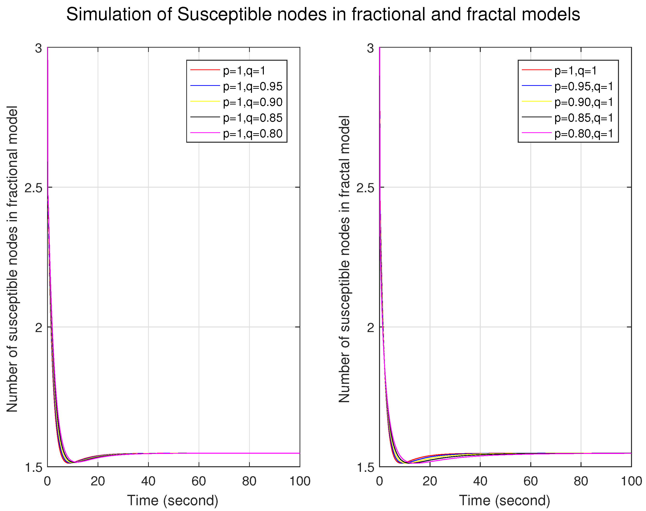
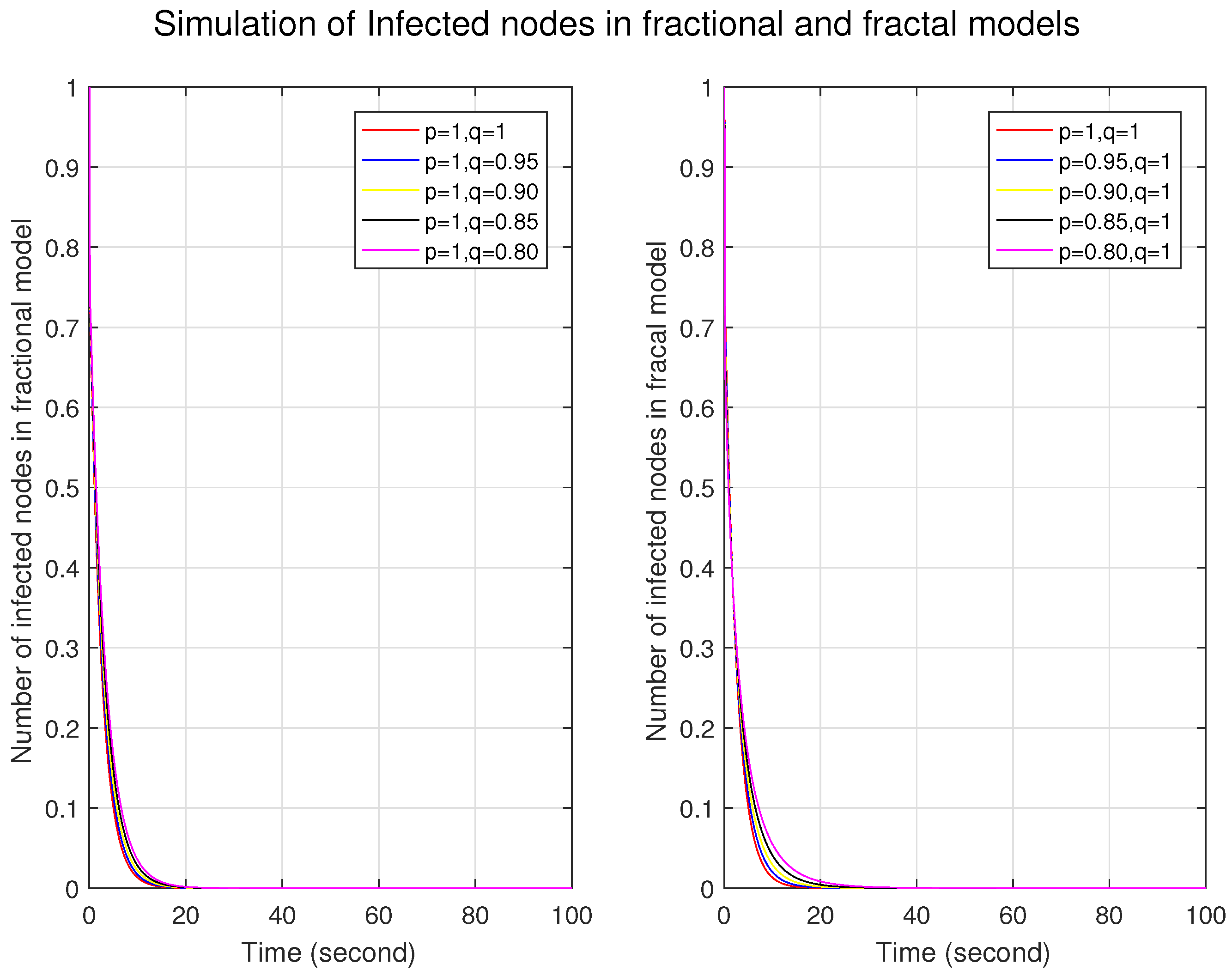
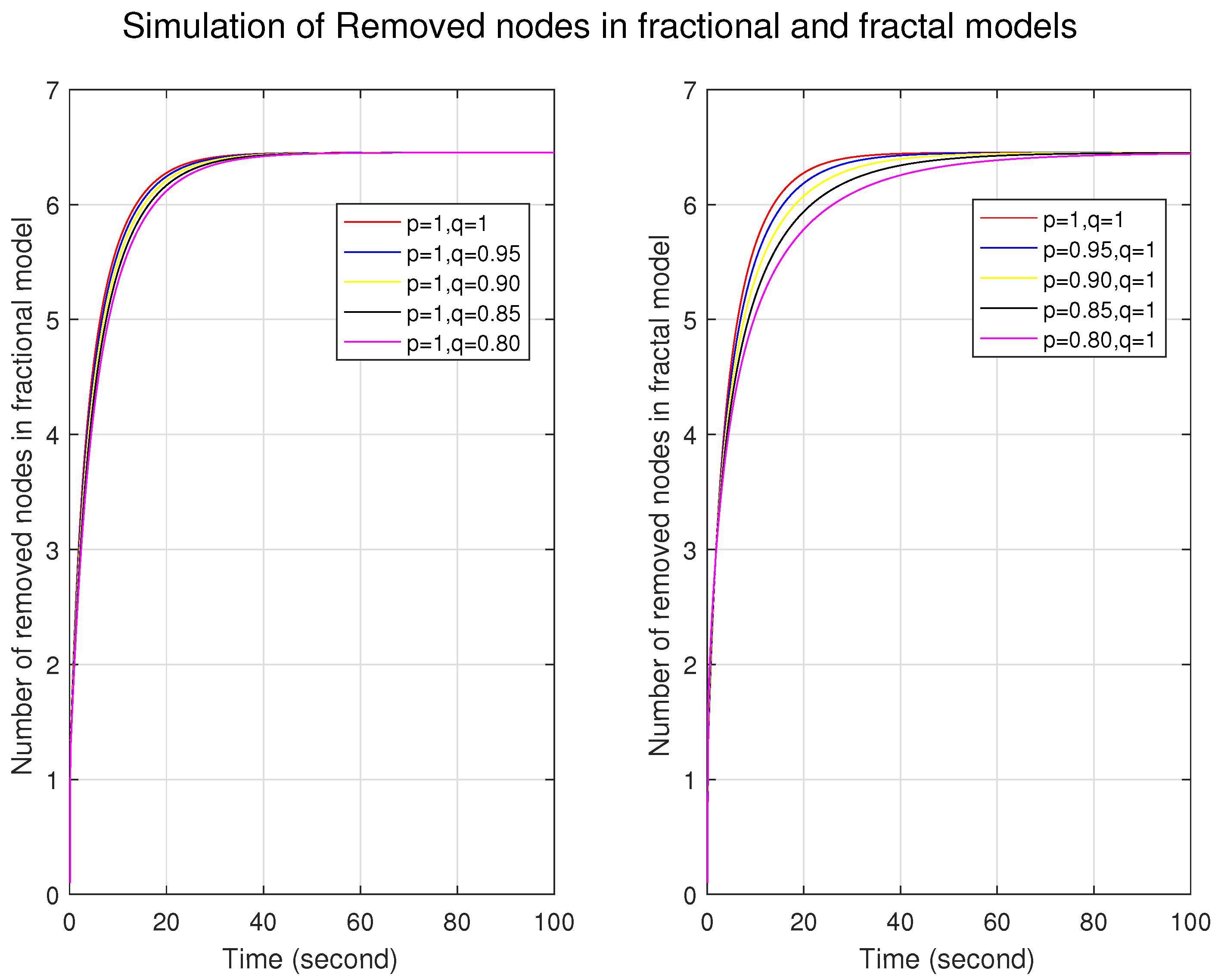
Figure 1, Figure 2 and 
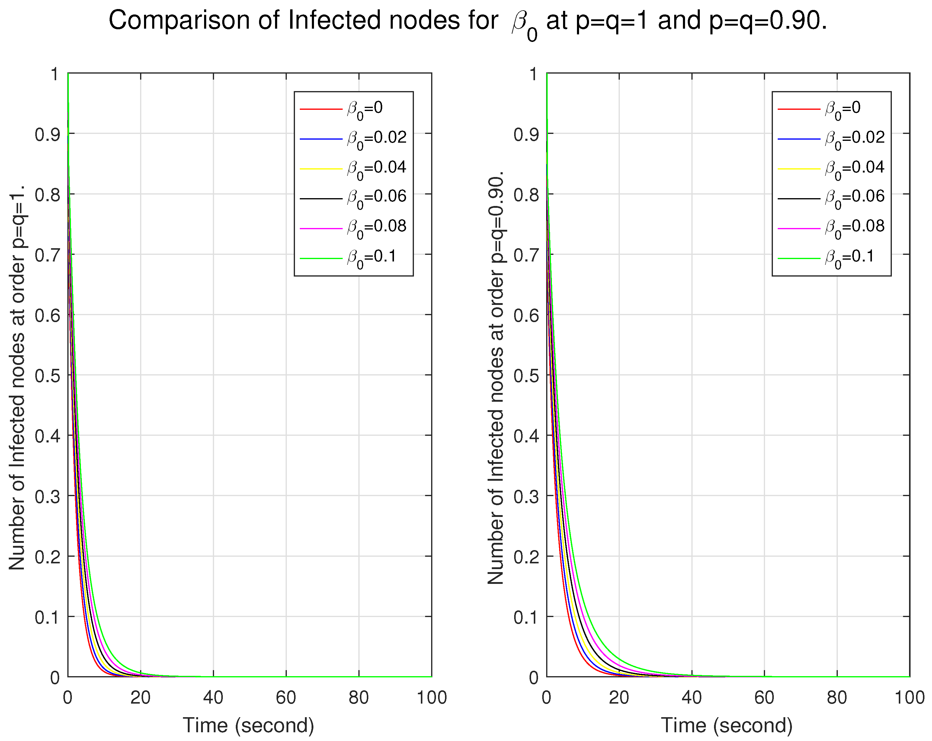
Figure 3 illustrate the simulations of the susceptible, infected, and removed nodes for the fractal and fractional models independently. First, we constructed a fractional model by taking different fractional orders with fractal orders of one. Similarly, the fractal model was built by taking different fractal orders with a fractional order of one. We can observe that the graphs for the trajectories of the nodes in the fractional model are very close to each other, which shows that the nodes are firmly connected and indicates a more homogeneous structure with fewer variations. In contrast, the distance between the nodes at different orders represents long-range corrections and depicts a more heterogeneous and complex structure. For fractal models, in Figure 1, initially at lower fractal orders, the number of nodes is more significant and then it decreases, which shows that, initially, the system has a strong memory effect and, as time passes, the memory effect decays. In Figure 2 and Figure 3, the number of infected nodes increases, and the number of removed nodes decreases for lower fractal orders. This shows that the system has a strong memory effect in the fractal model.
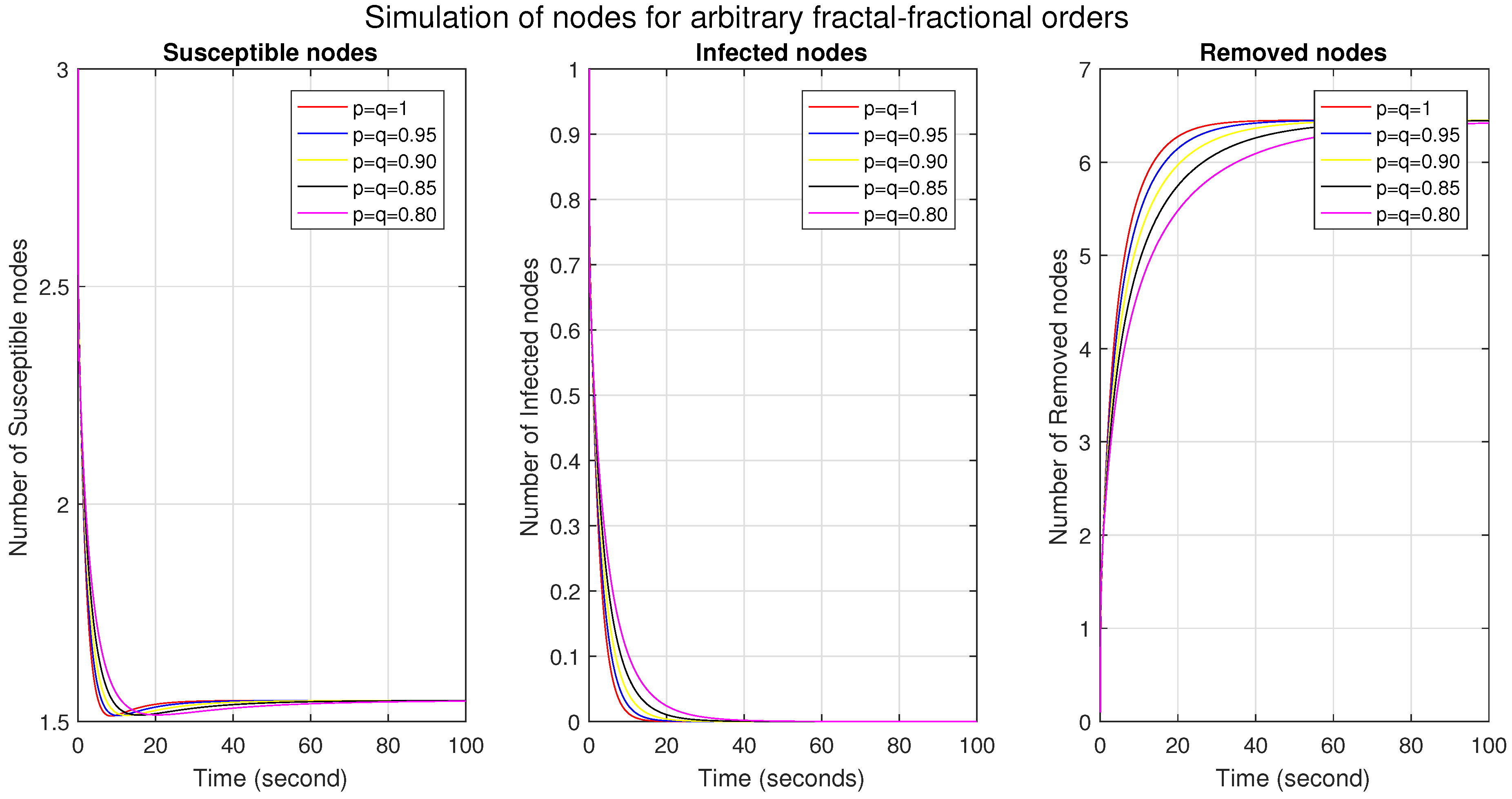
Figure 4 shows the simulations of the susceptible, infected, and removed/recovered nodes under the combined effect of different ff orders. We see that, in Figure 1, as the ff order decreases, the number of susceptible nodes is more significant initially, then decreases, and finally converges. This means that, initially, there is a higher degree of connectivity and vulnerability to infection; a decrease shows a reduction in both connectivity and vulnerability, probably due to increased immunity, and convergence shows that the system has become stable. The effect of the ff orders shows that the memory effect is stronger initially; after that, it decays with time. In Figure 2, the more significant number of nodes at lower ff orders indicates a more substantial memory effect and a higher potential for epidemic spread. We also observe that several infected nodes become zero early at higher ff orders, which indicates increased resilience and improved system immunity. It also indicates lower infection transmission rates and increased isolation. In Figure 3, the reduced number of removed nodes in the lower orders shows longer persistence, a higher prevalence of infection, and a longer and stronger memory effect. In Figure 5, we compare the classical and ff models, which shows the behavior of all nodes in a single figure.
Now, we show the impact of β 0 and α (involved in the function of ) in the classical and ff models. We examine the graphs in two ways. First, we discuss the behavior of the nodes for different ff orders in each model. Secondly, we compare the behavior of these nodes between the models. In Figure 6, as β 0 increases, the number of nodes also increases; this shows that the system may be more susceptible to infection, may exhibit a faster spread of infection due to a larger pool of infected nodes, and may show nonlinear dynamics, where small changes in β 0 lead to significant changes in the number of infected nodes. It also represents that the system has a more substantial memory effect. From the comparison, we see that in the lower ff model, the system is more flexible in becoming infectious and has a more significant memory effect. Here, the variable α varies proportionally to the sensitivity of infection, and α = 0 has a constant value. In Figure 7, we see the effect of this varying variable. Although there seems to be a slight difference, it plays a role in the system’s dynamics in coordination with other parameters.
In Figure 8, we see the effect of ν on Δ , , and Θ for the classical and ff models. The first column shows that as ν increases, each model’s number of susceptible nodes decreases. We can say that it shows a strong immune response, a decreased risk of infection, more resilience to infection, and the ability to eradicate infection. Moreover, comparing both models, we see that the number of nodes in the lower ff model is smaller. It shows increased complexity, slower spread of infection, increased clustering, improved resilience, and enhanced robustness. In the second column, the trajectories are very close to each other for different values of ν between the models. This depicts that the system may have reached a saturation point and exhibited diminishing returns. Also, for the ff model at 0.90, the number of nodes is greater, representing increased complexity, faster speed of infection, increased vulnerability, and reduced resilience. Similarly, in the third column, the number of removed nodes is greater for a higher real-time immune rate for both models. This shows an effective immune response capable of eliminating infected nodes efficiently, greater resilience in the system, and enhanced system robustness. From the comparison, we know that the number of nodes is less in the ff model at the 0.90 level, which results in a strong memory effect and increased system complexity.
Figure 9 shows the behavior of ζ (loss rate of immunity). From the first column, it can be seen that the number of susceptible nodes increases as the lost rate of immunity increases in both models. Furthermore, the ff model at 0.90 exhibits robustness to immunity loss and may introduce unique effects that mitigate the impact of immunity loss, producing an effective immune response with increased resilience. In the second column, the number of infected nodes remains the same for different rates of immunity loss in each model, showing that the immune response may have reached a saturation point, and the system reached an equilibrium state. It also shows the robustness and resilience of the system. Moreover, the number of infected nodes approaches zero earlier in the classical model. This means that the ff model at 0.90 shows a delayed eradication of infection, has a slower immune response, has lower efficiency, and has increased system vulnerability. Similarly, the number of removed nodes decreases with increasing loss of immunity in each model in the third column. This shows reduced immune efficiency, longer persistence, increased vulnerability, and reduced system resilience. Comparing the models, the ff model at 0.90 removes fewer nodes than the classical model, indicating impaired immune function, persistence of infection, vulnerability, and s decrease in system resilience.
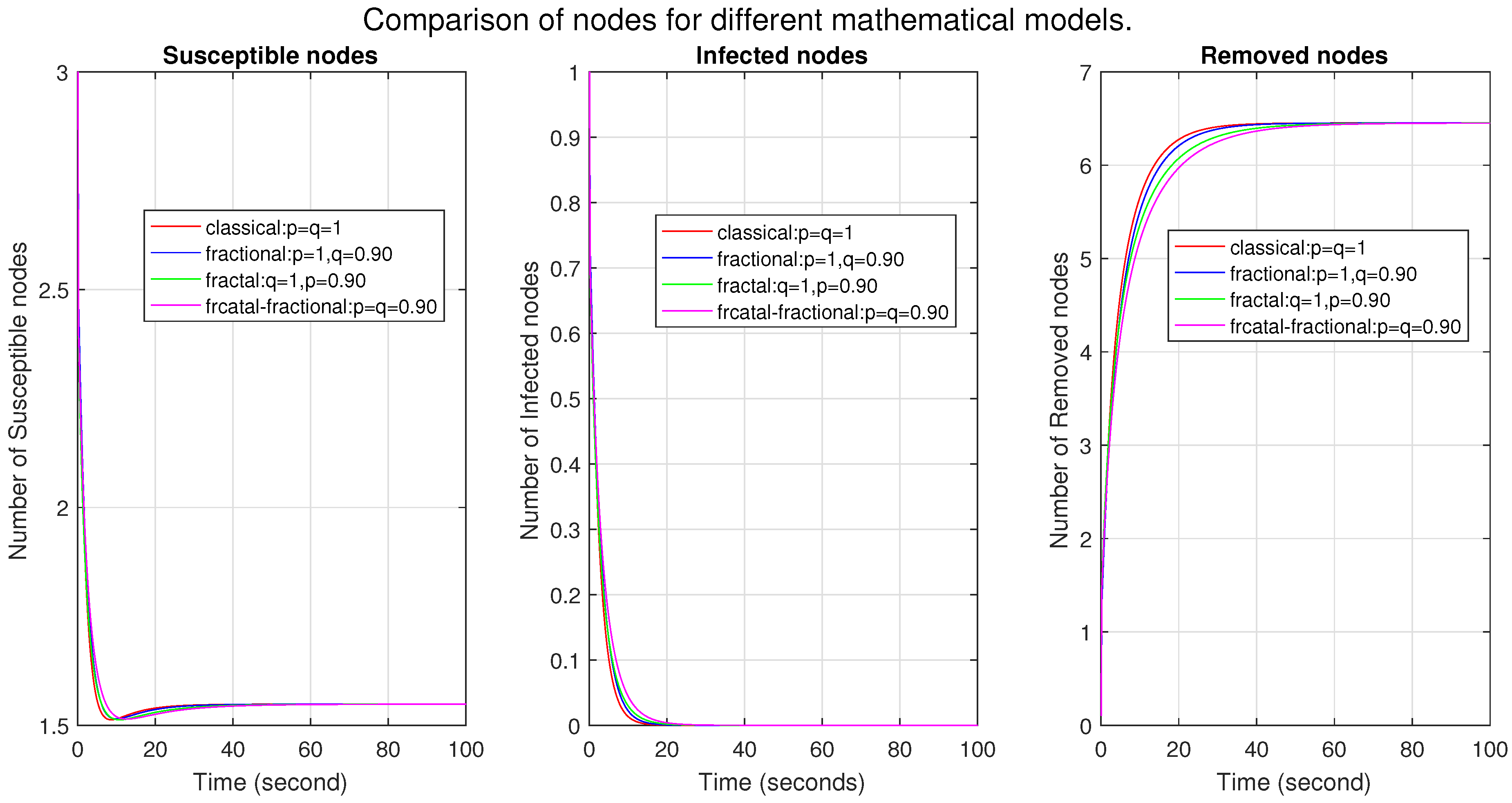
In Figure 10, we compare four mathematical models: classical, fractional, fractal, and fractal–fractional. The first two figures show that the number of susceptible and infected nodes is the highest in the ff model, then in the fractional, fractal, and classical models. This shows that the fractal–fractional model is more effective at expressing the complexity of malware propagation, and the fractional model may also be used in some cases. However, the fractal and classical methods are unsuitable for complex systems. The higher number of nodes represents a more profound memory effect and a strong correlation between nodes. Moreover, the convergence indicates that the system is stable. Similarly, in the third figure, the number of removed nodes in the fractal–fractional model is the lowest, which shows a strong memory effect and strong correlation. The convergence figure indicates the stability of the system. In 
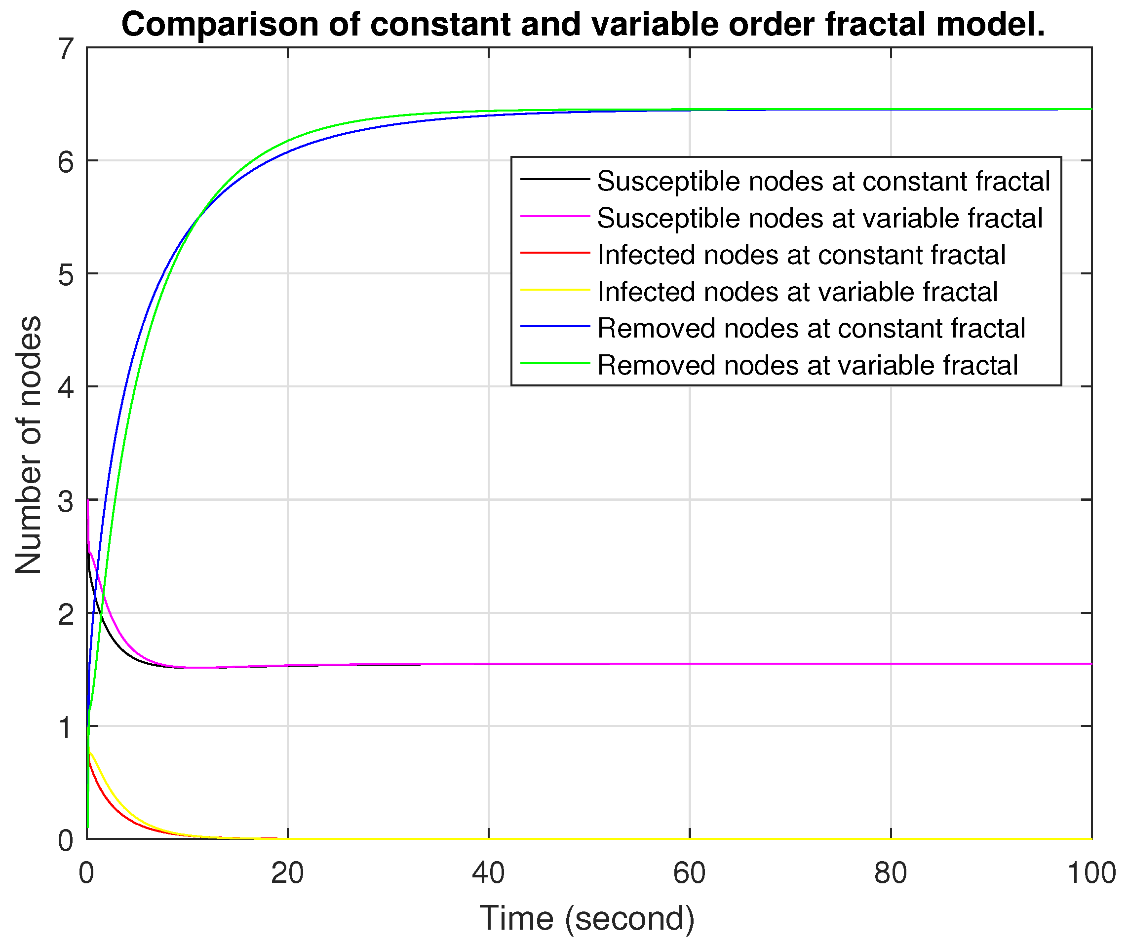
Figure 11, we see the difference between the constant and variable fractional orders. Similarly, Figure 12 compares the constant and variable fractal orders. We take the variable fractional order as q ( ϑ ) = 0.90 + 0.1 / ( 1 + e x p ( ϑ ) ) and the variable fractal order as p ( ϑ ) = 0.1 / 0.9 + e x p ( ϑ ) . As time passes, we see that the susceptible and infected nodes merge rapidly; this means that the variable order becomes constant. The number of nodes in the variable order is greater than in the constant order, indicating that the variable order provides an advantage in removing nodes, which leads to more effective epidemic control and a more adaptive system. The variable fractional and fractal orders represent more effective control strategies.

11. Conclusions

This paper discussed a mathematical deterministic model of malware propagation with a time-delay factor and a variable infection rate in the form of a fractal–fractional derivative. A classical mathematical model was converted into a fractal–fractional model with an exponential decay kernel and was formulated as a fixed-point problem, showing that the solution exists. Existence was examined using a theorem based on contraction ϕ ψ and the Leray–Schauder criteria. The uniqueness and stability were checked using the theorems defined for the ff model. Simulations were performed by creating a numerical scheme that verified our theory. Our F F model was examined as a fractional, fractal, and fractal–fractional model. The behavior of the nodes for lower FF orders explains the stronger memory effects, sensitivity to extrinsic factors, and flexibility to recover from infections. It also shows that the removed nodes achieve a greater confinement of infection and perseverance at lower levels of FF orders. We compared the ff model and the behavior of different parameters: β 0 , α , ν and ζ for p = q = 1 , and p = q = 0.90 . Observing the graphs, we explored the nodes’ sensitivity, convergence, stability, and memory effects. This predictive behavior may facilitate the identification of vulnerabilities in computer systems. It enables the development of antivirus strategies and specialized software to eliminate infections in network nodes. The graphs showed that the effects of malware can be managed by choosing appropriate parameters. We also compared four methods (classical, fractional, fractal, and fractal–fractional). We discussed the cases for which these models may be more suitably used. Moreover, we tried to determine the impact of variable-order fractional and variable-order fractal derivatives. Sometimes, we saw a minimal difference; it may play a role in malware propagation, as small changes may cause large perturbations. Our results may help develop cyber-security antivirus software through examining memory effects. Some forms of such malware are Nimda, red worms, Slammer worms, Witty worms (worms), Wanna Cry, NotPetya (Ransomware), Mirai, Srizbi(Botnets), and Zeus, Emotet (Trojans). Our method faces some limitations: the lack of adequate, accurate data and limited software package resources caused hurdles in evaluating the results. For future work, we are interested in exploring different advanced mathematical models concerning kernels, different computational algorithms, and different variable orders of derivatives to understand the propagation of malware. We also want access to accurate data so that this methodology can be used efficiently in cybersecurity systems.

Author Contributions

Conceptualization, N.R., A.B., U.I., T.K., M.G. and I.-L.P.; methodology, N.R., A.B., U.I., T.K., M.G. and I.-L.P.; software, N.R., A.B., U.I., T.K., M.G. and I.-L.P.; validation, N.R., A.B., U.I., T.K., M.G. and I.-L.P.; formal analysis, N.R., A.B., U.I., T.K., M.G. and I.-L.P.; investigation, N.R., A.B., U.I., T.K., M.G. and I.-L.P.; resources, N.R., A.B., U.I., T.K., M.G. and I.-L.P.; data curation, N.R., A.B., U.I., T.K., M.G. and I.-L.P.; writing—original draft preparation, N.R., A.B., U.I., T.K., M.G. and I.-L.P.; writing—review and editing, N.R., A.B., U.I., T.K., M.G. and I.-L.P.; visualization, N.R., A.B., U.I., T.K., M.G. and I.-L.P.; supervision, N.R., A.B., U.I., T.K., M.G. and I.-L.P.; project administration, N.R., A.B., U.I., T.K., M.G. and I.-L.P. All authors have read and agreed to the published version of this manuscript.

Funding

This research received no external funding.

Data Availability Statement

Data will be made available upon request from the corresponding author.

Acknowledgments

The authors extend their appreciation to King Saud University for funding this work through Researchers Supporting Project number (RSPD2025R1056), King Saud University, Riyadh, Saudi Arabia.

Conflicts of Interest

The authors declare no conflicts of interest.

References

  1. Megira, S.; Pangesti, A.R.; Wibowo, F.W. Malware analysis and detection using reverse engineering technique. J. Phys. Conf. Ser. 2018, 1140, 012042. [Google Scholar] [CrossRef]
  2. Pavithra, J.; Selvakumara Samy, S. A comparative study on detection of malware and benign on the internet using machine learning classifiers. Math. Probl. Eng. 2022, 2022, 4893390. [Google Scholar] [CrossRef]
  3. Maniriho, P.; Mahmood, A.N.; Chowdhury, M.J.M. A study on malicious software behaviour analysis and detection techniques: Taxonomy, current trends and challenges. Future Gener. Comput. Syst. 2022, 130, 1–18. [Google Scholar] [CrossRef]
  4. Akhtar, Z. Malware detection and analysis: Challenges and research opportunities. arXiv 2021, arXiv:2101.08429. [Google Scholar]
  5. Supriatna, A.K.; Husniah, H.; Anwar, R.H.; Hendayun, M. Mathematical Models of Malware Propagation: A Critical Level of Protection (CLoP). International Journal of Applied Mathematics and Statistics, Journal of Information, Jurnal Teknik Industri, Jurnal Teknologi, Computer Indusrtrial Engineering Journal and Many International Proceedings Published by IEEE, AIP, IOP, etc. Available online: https://www.researchgate.net/publication/340778616_Mathematical_Models_of_Malware_Propagation_A_Critical_Level_of_Protection_CLoP_-_Preprint (accessed on 11 December 2024).
  6. Attia, N.; Akgül, A.; Seba, D.; Nour, A.; Asad, J. A novel method for fractal-fractional differential equations. Alex. Eng. J. 2022, 61, 9733–9748. [Google Scholar] [CrossRef]
  7. Ross, B. A brief history and exposition of the fundamental theory of fractional calculus. In Fractional Calculus and Its Applications, Proceedings of the International Conference, West Haven, CT, USA, June 1974; Springer: Berlin/Heidelberg, Germany, 2006; pp. 1–36. [Google Scholar]
  8. Li, C.; Chen, Y.; Kurths, J. Fractional calculus and its applications. Philos. Trans. R. Soc. A Math. Phys. Eng. Sci. 2013, 371, 20130037. [Google Scholar] [CrossRef]
  9. Caputo, M.; Fabrizio, M. A new definition of fractional derivative without singular kernel. Prog. Fract. Differ. Appl. 2015, 1, 73–85. [Google Scholar]
  10. Atangana, A.; Baleanu, D. New fractional derivatives with nonlocal and non-singular kernel: Theory and application to heat transfer model. arXiv 2016, arXiv:1602.03408. [Google Scholar] [CrossRef]
  11. Atangana, A. Fractal-fractional differentiation and integration: Connecting fractal calculus and fractional calculus to predict complex system. Chaos Solitons Fractals 2017, 102, 396–406. [Google Scholar] [CrossRef]
  12. Yüksel, E. Some Fractal-Fractional Integral Inequalities for Different Kinds of Convex Functions. Kocaeli J. Sci. Eng. 2022, 5, 18–24. [Google Scholar] [CrossRef]
  13. Samet, B.; Vetro, C.; Vetro, P. Fixed point theorems for αψ-contractive type mappings. Nonlinear Anal. Theory Methods Appl. 2012, 75, 2154–2165. [Google Scholar] [CrossRef]
  14. Granas, A. Fixed Point Theory; Springer Monographs in Mathematics/Springer-Verlag: Berlin/Heidelberg, Germany, 2003. [Google Scholar]
  15. Mawhin, J. Leray-Schauder degree: A half century of extensions and applications. Topol. Methods Nonlinear Anal. 1999, 14, 195–228. [Google Scholar] [CrossRef]
  16. Lundquist, T. The Arzelá-Ascoli Theorem. Student’s Book Numerical Functional Analysis, 65. 2014. Available online: https://www2.it.uu.se/itwiki.php?page=education/phd_studies/phd_courses/NumFunkAnalysis_2014/NFAStudentBook.pdf&action=browse#page=67 (accessed on 11 December 2024).
  17. Rassias, T.M. On the stability of the linear mapping in Banach spaces. Proc. Am. Math. Soc. 1978, 72, 297–300. [Google Scholar] [CrossRef]
  18. Chen, W.; Sun, H.; Zhang, X.; Korošak, D. Anomalous diffusion modeling by fractal and fractional derivatives. Comput. Math. Appl. 2010, 59, 1754–1758. [Google Scholar] [CrossRef]
  19. Chen, W. Time–space fabric underlying anomalous diffusion. Chaos Solitons Fractals 2006, 28, 923–929. [Google Scholar] [CrossRef]
  20. Ahmad, S.; Ullah, A.; Akgül, A.; Baleanu, D. Theoretical and numerical analysis of fractal fractional model of tumor-immune interaction with two different kernels. Alex. Eng. J. 2022, 61, 5735–5752. [Google Scholar] [CrossRef]
  21. Srivastava, H.M.; Saad, K.M. Numerical simulation of the fractal-fractional Ebola virus. Fractal Fract. 2020, 4, 49. [Google Scholar] [CrossRef]
  22. Atangana, A.; Qureshi, S. Modeling attractors of chaotic dynamical systems with fractal–fractional operators. Chaos Solitons Fractals 2019, 123, 320–337. [Google Scholar] [CrossRef]
  23. Alqhtani, M.; Saad, K.M. Fractal–fractional Michaelis–Menten enzymatic reaction model via different kernels. Fractal Fract. 2021, 6, 13. [Google Scholar] [CrossRef]
  24. Rezapour, S.; Asamoah, J.K.K.; Hussain, A.; Ahmad, H.; Banerjee, R.; Etemad, S.; Botmart, T. A theoretical and numerical analysis of a fractal–fractional two-strain model of meningitis. Results Phys. 2022, 39, 105775. [Google Scholar] [CrossRef]
  25. Fatmawati; Khan, M.A.; Alfiniyah, C.; Alzahrani, E. Analysis of dengue model with fractal fractional Caputo Fabrizio operator. Adv. Differ. Equations 2020, 2020, 422. [Google Scholar] [CrossRef]
  26. Feng, L.; Liao, X.; Han, Q.; Li, H. Dynamical analysis and control strategies on malware propagation model. Appl. Math. Model. 2013, 37, 8225–8236. [Google Scholar] [CrossRef]
  27. Zheng, X.; Wang, H. Optimal-order error estimates of finite element approximations to variable-order time-fractional diffusion equations without regularity assumptions of the true solutions. IMA J. Numer. Anal. 2021, 41, 1522–1545. [Google Scholar] [CrossRef]
  28. Almutairi, N.; Saber, S. Application of a time-fractal fractional derivative with a power-law kernel to the Burke-Shaw system based on Newton’s interpolation polynomials. MethodsX 2024, 12, 102510. [Google Scholar] [CrossRef] [PubMed]
  29. Hyers, D.H. On the stability of the linear functional equation. Proc. Natl. Acad. Sci. USA 1941, 27, 222–224. [Google Scholar] [CrossRef] [PubMed]
Figure 1. Trajectories of Δ ( ϑ ) for fractional model and fractal model.
Fractalfract 09 00090 g001
Figure 2. Trajectories of ( ϑ ) for fractional model and fractal model.
Fractalfract 09 00090 g002
Figure 3. Trajectories of Θ ( ϑ ) for fractional model and fractal model.
Fractalfract 09 00090 g003
Figure 4. Fractal and fractional trajectories of Δ ( ϑ ) , ( ϑ ) , Θ ( ϑ ) for different orders of p = q .
Fractalfract 09 00090 g004
Figure 5. Comparison of Δ Θ model for classical and fractal–fractional method.
Fractalfract 09 00090 g005
Figure 6. The impact of varying initial infection rate β 0 on infected nodes in classical and ff model.
Fractalfract 09 00090 g006
Figure 7. The impact of α on infected nodes for classical and ff models.
Fractalfract 09 00090 g007
Figure 8. The impact of varying ν rates on susceptible, infected, and removed nodes in classical and ff models.
Fractalfract 09 00090 g008
Figure 9. The impact of varying loss rates of immunity ζ on susceptible, infected, and removed nodes in classical and ff models.
Fractalfract 09 00090 g009
Figure 10. Trajectories of Δ , , Θ for different mathematical models.
Fractalfract 09 00090 g010
Figure 11. Trajectories of Δ , and Θ , comparing constant and variable fractional mathematical models.
Fractalfract 09 00090 g011
Figure 12. Trajectories of Δ , and Θ , comparing of constant and variable fractal mathematical models.
Fractalfract 09 00090 g012
Table 1. Symbols and meanings of the variables and parameters of the model (1).
ParameterMeaning
Δ Susceptible nodes
Infected nodes
Θ Removed/recovered nodes
Π Susceptibility rate of new nodes
θ Number of new nodes
ζ Loss rate of immunity of the recovered nodes
σ Rate of replacement
ν Real-time immune rate of antivirus strategies
ρ Recovery rate of infected nodes
τ Change in time
β ( ϑ ) Infection rate at time ϑ
β 0 Initial infection rate
Table 2. The values of the parameters and initial conditions.
ParameterValue
Π 0.5
θ 0.8
ζ 0.01
σ 0.1
ν 0.2
ρ 0.2
τ 7.3
β 0 0.02
α 1
Δ ( 0 ) 3
( 0 ) 1
Θ ( 0 ) 0.1
Disclaimer/Publisher’s Note: The statements, opinions and data contained in all publications are solely those of the individual author(s) and contributor(s) and not of MDPI and/or the editor(s). MDPI and/or the editor(s) disclaim responsibility for any injury to people or property resulting from any ideas, methods, instructions or products referred to in the content.

