Fixed/Preassigned Time Synchronization of Impulsive Fractional-Order Reaction–Diffusion Bidirectional Associative Memory (BAM) Neural Networks

Abstract

This study delves into the synchronization issues of the impulsive fractional-order, mainly the Caputo derivative of the order between 0 and 1, bidirectional associative memory (BAM) neural networks incorporating the diffusion term at a fixed time (FXT) and a predefined time (PDT). Initially, this study presents certain characteristics of fractional-order calculus and several lemmas pertaining to the stability of general impulsive nonlinear systems, specifically focusing on FXT and PDT stability. Subsequently, we utilize a novel controller and Lyapunov functions to establish new sufficient criteria for achieving FXT and PDT synchronizations. Finally, a numerical simulation is presented to ascertain the theoretical dependency.

1. Introduction

Neural networks are a cornerstone of artificial intelligence, mimicking the human brain to address technological challenges and pave the way for new discoveries. These networks are instrumental in information processing, pattern classification, and cognitive control. Through mathematical modeling, we can examine and replicate brain functions in artificial systems, such as robotics. Both theoretical and practical research are essential to advance the field of dynamic neural networks.

Recently, fractional-order neural networks have become popular among scholars because fractional calculus can explain phenomena that classical calculus cannot, such as random errors and unusual diffusion processes. Their memory and hereditary properties make them valuable in various fields, including blood flow, electrolysis, and viscosity [1]. These fractional calculus properties, which allow neural networks to exhibit characteristics such as memory and heredity, demonstrate advantages over traditional integer-order derivatives when applied to various processes. These networks possess infinite memory, and the adjustment of the fractional parameters enhances the device output by increasing the degrees of freedom. They excel in information processing, parameter estimation, and diverse artificial intelligence applications and are comparable to biological networks [2,3] and geometric models [4]. Additionally, fractional-order derivatives offer more accurate depictions of chaotic behavior and a variety of nonlinear phenomena, because fractional-order derivatives exhibit global correlation and can better describe processes with strong historical dependence. Consequently, in recent years, a significant number of studies have been presented focusing on fractional-order chaotic systems [5,6]. With the increasing complexity of economic issues in the financial field, which are influenced by nonlinear factors, financial systems exhibit highly intricate phenomena. Therefore, it is essential to investigate the dynamic characteristics and effects of chaos in intricate financial systems [7]. Fractional-order models can better capture the complex behaviors and interactions within financial markets or provide more accurate risk assessments and predictions. In [8], variable-order time-fractional generalized Navier–Stokes equations were introduced to describe the anomalous dynamics in porous flows to reveal the impact of the fractional order on fluid flow in porous media. Other works detailed the use of fractional-order systems in the encryption of images [9,10,11].

On the other hand, in various scientific domains, including image encryption [12,13], pattern formation, biology [14] and chemistry, reaction–diffusion terms are indispensable. In particular, bidirectional associative memory (BAM) neural networks with reaction–diffusion terms enhances their ability to store and recall the associations between input and output patterns, making them effective tools for pattern recognition [15] and associative memory tasks [16]. Ali et al. [17] examined the synchronization of fractional-order BAM neural networks with fuzzy terms and time-varying delays by presenting sufficient conditions. Lin et al. [18] investigated the synchronization of issue of BAM neural networks with diffusion and time-varying delays and achieved spatio-temporal synchronization by proposing an impulsive pinning controller. Chen et al. [19] investigated the global exponential synchronization for BAM neural memristive neural networks with mixed delays and reaction–reaction diffusion terms based on a new integral inequality with an infinite distributed delay. Furthermore, in certain networks, especially biological neural networks, there are instances where we must precisely capture the propagation of electrical signals and the diffusion of neurotransmitters within a neuron network. To achieve this, we must consider the impact of previous states and the spatial arrangement of neurons. Therefore, we will focus on fractional-order BAM neural networks subject to reaction–diffusion terms.

However, in the aforementioned studies, they neglected abrupt changes in the system. Many motion processes in nature undergo sudden changes compared with the entire motion process, and the duration of these abrupt changes is very short; we refer to this phenomenon as impulse effects. Impulse effects are significant in many engineering systems, such as instantaneous transitions or resets in system states, video encoding, image encryption [20,21], and natural language processing [22]. Several studies have been conducted on impulse phenomena [16,22,23]. In [23], the synchronization of linearly coupled memristor-based recurrent neural networks with impulses was investigated. In [22], the authors provided sufficient conditions for the asymptotic stability of impulse stochastic systems. In [16], new stability criteria for reaction–diffusion impulsive neural networks were developed.

Synchronization is also a critical element in numerous natural processes, and it holds paramount importance within neural network systems. The analysis of the synchronization between two systems can be encapsulated in the stability of an error system. Particularly in the realm of fractional-order neural networks, synchronization is vital for preserving the stability, performance, and communication among linked networks. It improves the precision and efficiency of computations, enhancing performance in tasks such as signal processing, pattern recognition, and control systems. Many studies have explored this field; for instance, Pratap et al. [24] investigated the asymptotic synchronization of Cohen–Grossberg fractional-order neural networks and confirmed the global existence of asymptotically stable solutions. Velmurugan et al. [25] analyzed finite-time synchronization conditions for fractional-order memristor-based neural networks using Laplace transforms and Mittag–Leffler functions. Subsequently, Du and Lu [26] introduced a fractional-order Gronwall inequality for finite-time synchronization of fractional-order memristor-based neural networks with a time delay. However, finite-time synchronization has limitations such as the settling time depending on the initial conditions, which are often unknown in practical applications, complicating the determination of precise convergence times. To address these limitations, the concept of fixed-time (FXT) stability was introduced by Polyakov [27] and has been applied to various neural network systems, including those of fractional-order, with reaction–diffusion and impulsive terms [5,6,7,20]. Nevertheless, there is a paucity of studies on the synchronization of fractional-order impulsive neural networks incorporating reaction–diffusion terms. Building upon preceding work, this study explores the FXT and predefined-time (PDT) synchronizations in impulsive fractional-order systems with reaction–diffusion components. The main contributions of this study are as follows:

• We present a novel controller to establish a sufficient condition for reaching FXT and PDT synchronizations in fractional-order impulsive neural networks with diffusion terms.
• We establish the robustness of the FXT and PDT synchronization approaches against fluctuations in parameter configurations.
• We demonstrate the influence of the fractional-order parameter on the synchronization of the given system.

The organization of the paper is laid out as follows: Section 2 provides the necessary definitions, lemmas, and details of the systems under study, which are vital for the proof of the main results in the following section. Section 3 describes the design of a new controller intended for FXT and PDT synchronizations in impulsive reaction–diffusion fractional-order neural networks. Section 4 presents an evaluation of the effectiveness of the theoretical findings introduced in this study. Finally, Section 5 concludes the paper with a summary of the main points.

2. Preliminaries

2.1. Theoretical Background

The study of fractional-order derivatives has gained prominence with the development of mathematical analysis. There are various definitions of fractional-order derivatives, including the Caputo derivative and Riemann–Liouville’s derivative. The specific definition is as follows [28]:

• Riemann–Liouville integral for $\alpha \in (0,1)$:

  $$\begin{array}{c}\hfill I^{\alpha }x(t)={\displaystyle \frac{1}{\Gamma (\alpha )}}{\int }_0^t{\displaystyle \frac{x(\theta )}{{(t-\theta )}^{1-\alpha }}}d\theta .\end{array}$$
• Riemann–Liouville derivative for $\alpha \in (0,1)$:

  $$\begin{array}{c}\hfill {⠀}^{RL}{D}^{\alpha }x(t)={\displaystyle \frac{d}{dt}}{I}^{1-\alpha }x(t)={\displaystyle \frac{1}{\Gamma (1-\alpha )}}{\displaystyle \frac{d}{dt}}{\int }_0^t{\displaystyle \frac{x(\theta )-x(0)}{{(t-\theta )}^{\alpha }}}d\theta .\end{array}$$
• Caputo derivative:

  $$\begin{array}{c}\hfill D^{\alpha }x(t)={\displaystyle \frac{1}{\Gamma (1-\alpha )}}{\int }_0^t{\displaystyle \frac{x^{\prime }(\theta )}{{(t-\theta )}^{\alpha }}}d\theta ,0<\alpha <1,\\ \hfill D^{\alpha }x(t)={\displaystyle \frac{1}{\Gamma (1-\alpha )}}{\int }_0^t{\displaystyle \frac{x^{\prime }(\theta )}{{(t-\theta )}^{1-m+\alpha }}}d\theta ,m-1<\alpha <m.\end{array}$$

Our main concentration is on the Caputo derivative with order $\alpha \in (0,1)$. We will now present lemmas and properties that facilitate the derivation of the main results.

Property 1 

([29]). The following property can potentially be met for $\alpha >0,\beta >0$,

$$D^{\alpha }\left(I^{\beta }x(t)\right)=D^{\alpha -\beta }x(t).$$

Property 2 

([30]). The Caputo fractional derivative of the $|x(t)|$ satisfies the following inequality:

$$D^{\alpha }|x(t)|\le \mathrm{sign}(x(t))D^{\alpha }x(t),$$

where $0<\alpha <1$, $x(t)\in C^1[0,\infty )$.

Lemma 1 

([31]). The equality

$$\begin{array}{c}\hfill {⠀}^{RL}{D}_t^{\alpha }x(t)=D_t^{\alpha }x(t)+{\displaystyle \frac{x(0)}{\Gamma (1-\alpha )t^{\alpha }}}\end{array}$$

holds true if $x(t)\in C[0,\infty )$. Where, $0<\alpha <1$.

Lemma 2 

([32]). Given that $0<a\le 1$, $b>1$, and $z_i>0$ for $i=1,2,\cdots ,k$, the subsequent inequalities are valid:

$$\begin{array}{c}\hfill \sum _{i=1}^k{z}_i^a\ge {(\sum _{i=1}^k{z}_i)}^a,\sum _{i=1}^k{z}_i^b\ge k^{1-b}{(\sum _{i=1}^k{z}_i)}^b.\end{array}$$

2.2. System Description

Throughout this study, we consider the following class of nonlinear impulsive neural networks characterized by fractional-order dynamics and the inclusion of diffusion terms:

$$\left\{\begin{array}{ccc}{D}_t^{\alpha }{v}_{\iota }(t,x)=d_{\iota }\Delta v_{\iota }(t,x)-a_{\iota }{v}_{\iota }(t,x)+\sum _{\kappa =1}^m{b}_{\iota \kappa }{h}_{\kappa }(w_{\kappa }(t,x))+I_{\iota },\hfill & \hfill & t\ne t_{\tau },\hfill \\ D_t^{\alpha }{w}_{\kappa }(t,x)={\widehat{d}}_{\kappa }\Delta w_{\kappa }(t,x)-{\widehat{a}}_{\kappa }{w}_{\kappa }(t,x)+\sum _{\iota =1}^n{\widehat{b}}_{\kappa \iota }{\widehat{h}}_{\iota }(v_{\iota }(t,x))+{\widehat{I}}_{\kappa },\hfill & \hfill & t\ne t_{\tau },\hfill \\ v_{\iota }(t_{\tau }^{+},x)={\displaystyle \frac{{\xi }_{\iota }}{\Gamma (2-\alpha )}}{v}_{\iota }(t_{\tau },x),\hfill & \hfill & t=t_{\tau },\hfill \\ w_{\kappa }(t_{\tau }^{+},x)={\displaystyle \frac{{\widehat{\xi }}_{\kappa }}{\Gamma (2-\alpha )}}{w}_{\kappa }(t_{\tau },x),\hfill & \hfill & t=t_{\tau },\hfill \end{array}\right.$$

(1)

for $\iota \in \mathfrak{I}=\{1,2,\cdots ,n\}$, $\kappa \in \mathfrak{J}=\{1,2,\cdots ,m\}$, where the numbers of neurons are represented by n and m, $\Delta \mu ={\sum }_{h=1}^l{\displaystyle \frac{d^2\mu }{d{x}_h^2}}$, and l is the space dimension. The state variables for the $\iota$th neuron and the $\kappa$th neuron at time t and spatial location x are represented by $v_{\iota }(t,x)\in R$ and $w_{\kappa }(t,x)\in R$, respectively. The self-inhibition rates of the neurons are denoted by the positive constants $a_{\iota }$ and ${\widehat{a}}_{\kappa }$. The synaptic connection weights are represented by the constants $b_{\iota \kappa }$ and ${\widehat{b}}_{\kappa \iota }$. The activation functions for the neurons are $h_{\iota }(·)$ and ${\widehat{h}}_{\kappa }(·)$. The biases of the neurons are given by the variables $I_{\iota }$ and ${\widehat{I}}_{\kappa }$. Additionally, ${\xi }_{\iota }$ and ${\widehat{\xi }}_{\kappa }$ are positive constants. The functions $v_{\iota }(t_{\tau }^{+},x)$ and $w_{\kappa }(t_{\tau }^{+},x)$ describe the impulse jumps that take place at the specific impulse moments $t_{\tau }$$(\tau =1,2,3,\cdots )$. The sequence $\left\{t_{\tau }\right\}$ is strictly increasing and satisfies the condition ${lim}_{\tau \to +\infty }{t}_{\tau }=+\infty$.

The initial and boundary conditions for the system (1) are detailed as

$$\left\{\begin{array}{c}{v}_{\iota }(0,x)=v_{\iota }^0(x),\hfill \\ w_{\kappa }(0,x)=w_{\kappa }^0(x),\hfill \end{array}\right.\mathrm{for}x\in \Omega ,$$

$$\left\{\begin{array}{c}{\displaystyle \frac{\partial v_{\iota }(t,x)}{\partial \nu }}=0,\hfill \\ {\displaystyle \frac{\partial w_{\kappa }(t,x)}{\partial \nu }}=0,\hfill \end{array}\right.\mathrm{for}(t,x)\in (0,+\infty )\times \partial \Omega ,$$

for $\iota \in \mathfrak{I}$, $\kappa \in \mathfrak{J}$, where $v_{\iota }^0$ and $w_{\kappa }^0$ are bounded continuous functions.

The response system for the drive system can be introduced as

$$\left\{\begin{array}{ccc}{D}_t^{\alpha }{v}_{\iota }^{*}(t,x)=d_{\iota }\Delta v_{\iota }^{*}(t,x)-a_{\iota }{v}_{\iota }^{*}(t,x)+\sum _{\kappa =1}^m{b}_{\iota \kappa }{h}_{\kappa }(w_{\kappa }^{*}(t,x))+I_{\iota }+u_{\iota }(t,x),\hfill & \hfill & t\ne t_{\tau },\hfill \\ D_t^{\alpha }{w}_{\kappa }^{*}(t,x)={\widehat{d}}_{\kappa }\Delta w_{\kappa }^{*}(t,x)-{\widehat{a}}_{\kappa }{w}_{\kappa }^{*}(t,x)+\sum _{\iota =1}^n{\widehat{b}}_{\kappa \iota }{\widehat{h}}_{\iota }(v_{\iota }^{*}(t,x))+{\widehat{I}}_{\kappa }+{\widehat{u}}_{\kappa }(t,x),\hfill & \hfill & t\ne t_{\tau },\hfill \\ v_{\iota }^{*}(t_{\tau }^{+},x)={\displaystyle \frac{{\xi }_{\iota }}{\Gamma (2-\alpha )}}{v}_{\iota }^{*}(t_{\tau },x),\hfill & \hfill & t=t_{\tau },\hfill \\ w_{\kappa }^{*}(t_{\tau }^{+},x)={\displaystyle \frac{{\widehat{\xi }}_{\kappa }}{\Gamma (2-\alpha )}}{w}_{\kappa }^{*}(t_{\tau },x),\hfill \end{array}\right.$$

(2)

for $\iota \in \mathfrak{I}$, $\kappa \in \mathfrak{J}$. Where, $v_{\iota }^{*}(t,x)\in R$ and $w_{\kappa }^{*}(t,x)$ represent the state variables of the system (2). The controllers, denoted as $u_{\iota }(t,x)$, ${\widehat{u}}_{\kappa }(t,x)$, will be designed in the subsequent section.

The initial and boundary conditions for the system (2) are detailed as

$$\left\{\begin{array}{c}{v}_{\iota }^{*}(0,x)=v_{\iota }^{*0}(x),\hfill \\ w_{\kappa }^{*}(0,x)=w_{\kappa }^{*0}(x),\hfill \end{array}\right.\mathrm{for}x\in \Omega ,$$

$$\left\{\begin{array}{c}{\displaystyle \frac{\partial v_{\iota }^{*}(t,x)}{\partial \nu }}=0,\hfill \\ {\displaystyle \frac{\partial w_{\kappa }^{*}(t,x)}{\partial \nu }}=0,\hfill \end{array}\right.\mathrm{for}(t,x)\in (0,+\infty )\times \partial \Omega ,$$

where the functions $v_{\iota }^{*0}(·)$ and $w_{\kappa }^{*0}(·)$ are both continuous and bounded. Let $\iota \in \mathfrak{I}$, $\kappa \in \mathfrak{J}$, and the paper maintains the following consistent assumptions.

Assumption 1. 

There exist constants $L_i>0$$(i=1,2,\cdots ,n)$ and ${\widehat{L}}_j>0$$(j=1,2,\cdots ,m)$ such that the activation functions $h_i(·)$ and ${\widehat{h}}_i(·)$ satisfy

$$\begin{array}{c}|h_i(a_1)-h_i(a_2)|\le L_i|a_1-a_2|,\hfill \\ |{\widehat{h}}_j(a_1)-{\widehat{h}}_j(a_2)|\le {\widehat{L}}_j|a_1-a_2|,\hfill \end{array}$$

where $a_1$ and $a_2$ are arbitrary real constants.

The error system of (1) and (2) is

$$\left\{\begin{array}{ccc}{D}_t^{\alpha }{\epsilon }_{\iota }(t,x)=d_{\iota }\Delta {\epsilon }_{\iota }(t,x)-a_{\iota }{\epsilon }_{\iota }(t,x)+\sum _{\kappa =1}^m{b}_{\iota \kappa }{H}_{\kappa }({\eta }_{\kappa }(t,x))+u_{\iota },\hfill & \hfill & t\ne t_{\tau },\hfill \\ D_t^{\alpha }{\eta }_{\kappa }(t,x)={\widehat{d}}_{\kappa }\Delta {\eta }_{\kappa }(t,x)-{\widehat{a}}_{\kappa }{\eta }_{\kappa }(t,x)+\sum _{\iota =1}^n{\widehat{b}}_{\kappa \iota }{\widehat{H}}_{\iota }({\epsilon }_{\iota }(t,x))+{\widehat{u}}_{\kappa },\hfill & \hfill & t\ne t_{\tau },\hfill \\ {\epsilon }_{\iota }(t_{\tau }^{+},x)={\displaystyle \frac{{\xi }_{\iota }}{\Gamma (2-\alpha )}}{\epsilon }_{\iota }(t_{\tau },x),\hfill & \hfill & t=t_{\tau },\hfill \\ {\eta }_{\kappa }(t_{\tau }^{+},x)={\displaystyle \frac{{\widehat{\xi }}_{\kappa }}{\Gamma (2-\alpha )}}{\eta }_{\kappa }(t_{\tau },x),\hfill & \hfill & t=t_{\tau },\hfill \end{array}\right.$$

(3)

where

$$\begin{array}{c}{\epsilon }_{\iota }(t,x)=v_{\iota }^{*}(t,x)-v_{\iota }(t,x),\hfill \\ {\eta }_{\kappa }(t,x)=w_{\kappa }^{*}(t,x)-w_{\kappa }(t,x),\hfill \\ H_{\kappa }\left({\eta }_{\kappa }(t,x)\right)=h_{\kappa }\left(w_{\kappa }^{*}(t,x)\right)-h_{\kappa }\left(w_{\kappa }(t,x)\right),\hfill \\ {\widehat{H}}_{\iota }\left({\epsilon }_{\iota }(t,x)\right)={\widehat{h}}_{\iota }\left(v_{\iota }^{*}(t,x)\right)-{\widehat{h}}_{\iota }\left(v_{\iota }(t,x)\right),\hfill \end{array}$$

for $\iota \in \mathfrak{I}$, $\kappa \in \mathfrak{J}$.

Here. we delineate the essential definitions and supporting lemmas that form the basis of our main results. Consider the system described below:

$$\begin{array}{c}{\displaystyle \frac{d}{dt}}\phi (t)=\mathcal{F}(t,\phi (t)),t\ne t_{\tau },\hfill \\ \phi (0)={\phi }_0,\hfill \\ {\Delta \phi |}_{t=t_{\tau }}=\Lambda (t_{\tau },\phi (t_{\tau })),t_{\tau }\in N,\hfill \end{array}$$

(4)

where the state vector of the system denoted by $\phi (t)\in R^n$. $\mathcal{F}:R^{+}\times R^n\to R^n$ is a given continuous function with the condition that $\mathcal{F}(0,\phi (0))=0$. $\Lambda :R^{+}\times R^n=R^n$ is a function that is both continuously differentiable and locally Lipschitz and meets the condition $\Lambda (t,0)=0$.

Definition 1 

([32,33]). The zero solution of the system (4) is called FXT-stable if the solution $\phi (t,{\phi }_0)$ starting from the initial condition ${\phi }_0\in R^n$ meets the following criteria:

(i) 

Lyapunov stable. For any $\epsilon >0$, there is a $\delta =\delta (\epsilon )>0$ such that $\parallel \phi (t,{\phi }_0)\parallel <\epsilon$ for any $\parallel {\phi }_0\parallel \le \delta$ and $t\ge 0$;

(ii) 

Finite-time convergence. There exists a function $T:R^n\setminus 0\to (0,+\infty )$, called the settling time (ST) function, such that ${lim}_{t\to T({\phi }_0)}\phi (t,{\phi }_0)=0$ and $\phi (t,{\phi }_0)=0$ for all $t\ge T({\phi }_0)$;

(iii) 

$T({\phi }_0)$ is bounded. There exist $T_{\max }>0$ such that $T({\phi }_0)\le T_{\max }$ for all ${\phi }_0\in R^n$.

Definition 2 

([34]). The zero solution of system (4) is PDT-stable if it exhibits FXT stability for any initial condition ${\phi }_0\in R^n$ and for any given time $T_c>0$ $T({\phi }_0)\le T_c$ holds true.

Lemma 3 

([33]). If a Lyapunov function $V(t,\phi (t))$ exists and satisfies

(i) 

${\epsilon }_1{\parallel \phi (t)\parallel }^2\le V(t,\phi (t))\le {\epsilon }_2{\parallel \phi (t)\parallel }^2$, $\forall t\in R^{+},\phi \in R^n$;

(ii) 

$$\left\{\begin{array}{c}\dot{V}(t,\phi (t))\le -\mu V^p(t,\phi (t))-\lambda V^q(t,\phi (t)),t\ne t_{\tau },\hfill \\ V(t^{+},\phi (t_{\tau }^{+}))\le \Lambda V(t_{\tau },\phi (t_{\tau })),t=t_{\tau },\hfill \end{array}\right.$$

(5)

where ${\epsilon }_1,{\epsilon }_2,K,\mu ,\lambda$ are positive scalars, $0<p<1$, $q>1$ and $0<\Lambda \le 1$. Then, the system (4) is FXT-stable with the ST

$$\begin{array}{c}\hfill T_1=2{\nu }_{\tau }{N}_0+{\displaystyle \frac{1}{(1-p)\eta }}ln{\displaystyle \frac{\mu }{\mu -\eta }}+{\displaystyle \frac{1}{(1-q)\eta }}ln\left(1-{\displaystyle \frac{\eta {\Lambda }^{N_0(1-q)}}{\lambda }}\right)\end{array}$$

where $\eta ={\displaystyle \frac{ln\Lambda }{{\nu }_{\tau }}}$.

In Lemma 3, ${\nu }_{\tau }$ denotes the average impulse interval, and $N_0$ is a positive constant. For the detailed definitions of ${\nu }_{\tau }$ and $N_0$, refer to Definition 2 in the reference [32].

Lemma 4 

([34]). If a Lyapunov function $V(t,\phi (t))$ exists and satisfies:]

(i) 

${\epsilon }_1{\parallel \phi (t)\parallel }^2\le V(t,\phi (t))\le {\epsilon }_2{\parallel \phi (t)\parallel }^2$, $\forall t\in R^{+},\phi \in R^n$;

(ii) 

$$\left\{\begin{array}{c}\dot{V}(t,\phi (t))\le -{\displaystyle \frac{T_0}{T_c}}\left(\mu V^p(t,\phi (t))+\lambda V^q(t,\phi (t))\right),t\ne t_{\tau },\hfill \\ V(t^{+},\phi (t_{\tau }^{+}))\le \Lambda V(t_{\tau },\phi (t_{\tau })),t=t_{\tau },\hfill \end{array}\right.$$

(6)

then the system (4) will be PDT-stable with a preassigned time $T_c$, where $T_0$ is given as $T_0={\displaystyle \frac{1}{\mu (1-p){\pi }^2}}+{\displaystyle \frac{1}{\lambda (q-1)\varpi }}$, $\varpi ={\Lambda }^{-{\tau }^0(1-\gamma )}$, $\pi ={\Lambda }^{{\tau }^0(1-p)}$. ${\epsilon }_1,{\epsilon }_2,K,\mu ,\lambda ,p,q$ are described in Lemma 3.

2.3. Fractional-Order Lyapunov Exponent

Lyapunov exponents are invaluable tools for characterizing chaos, analyzing stability, predicting critical transitions, and efficiently computing the properties of chaotic attractors. Their applications extend from theoretical studies to practical data-driven approaches in various scientific fields. For example, the largest Lyapunov exponent determines the dominant rate of divergence or convergence of trajectories, while the full spectrum of Lyapunov exponents can reveal the overall stability characteristics of the system. In chaotic systems, the presence of at least one positive Lyapunov exponent confirms the existence of chaotic dynamics [35,36]. Now, we introduce the Lyapunov exponent for a fractional-order system $D_t^{\alpha }\Phi =\mathbf{f}(\Phi (t))$, where $\Phi (t)=({\varphi }_1,{\varphi }_2,\cdots ,{\varphi }_n)$, $\mathbf{f}(\Phi (t))=(f({\varphi }_1),f({\varphi }_2),\cdots ,f({\varphi }_n))$ are real-valued n-dimensional vector. Then, its Lyapunov exponents can be introduced as [35]

$$\begin{array}{c}{a}_{ij}^{(k)}=\Delta t^{\alpha }{\displaystyle \frac{\partial f_i}{\partial {\varphi }_j}}{a}_{ij}^{(k-1)}-\sum _{\ell =1}^{k+1}{\omega }_l{a}_{ij}^{(k-\ell )},\hfill \\ {\lambda }_j=\underset{k\to \infty }{lim}{\displaystyle \frac{1}{kh}}ln\parallel {\mathbf{a}}_j^{(k)}\parallel ,\hfill \end{array}$$

with ${\omega }_{\ell }=(1-{\displaystyle \frac{1+\alpha }{\ell }}){\omega }_{\ell -1}$, and initial value $({\mathbf{a}}_1^{(0)},{\mathbf{a}}_2^{(0)},\cdots ,{\mathbf{a}}_j^{(0)},\cdots ,{\mathbf{a}}_n^{(0)})=I$ (I is n identity matrix). For more specific information, please refer to work [35].

3. Main Results

We present a pair of pivotal theorems that are instrumental in achieving FXT and PDT synchronizations within the system under consideration.

3.1. FXT Synchronization

The controllers $u_{\iota }(t)$ and ${\widehat{u}}_{\kappa }(t)$ are designed as

$$\begin{array}{cc}\hfill u_{\iota }(t,x)=& -{\delta }_{\iota }{\epsilon }_{\iota }(t,x)-[{\theta }_{\iota }{\tilde{\epsilon }}^{{\displaystyle \frac{p-1}{2}}}(t)D_t^{\alpha -1}|{\epsilon }_{\iota }(t,x)|\hfill \\ \hfill & +{\vartheta }_{\iota }{\tilde{\epsilon }}^{{\displaystyle \frac{q-1}{2}}}(t)D_t^{\alpha -1}|{\epsilon }_{\iota }(t,x)|]\mathrm{sign}({\epsilon }_{\iota }(t,x)),\hfill \\ \hfill {\widehat{u}}_{\kappa }(t,x)=& -{\widehat{\delta }}_{\kappa }{\eta }_{\kappa }(t,x)-[{\widehat{\theta }}_{\kappa }{\tilde{\eta }}^{{\displaystyle \frac{p-1}{2}}}(t)D_t^{\alpha -1}|{\eta }_{\kappa }(t,x)|\hfill \\ \hfill & +{\widehat{\vartheta }}_{\kappa }{\tilde{\eta }}^{{\displaystyle \frac{q-1}{2}}}(t)D_t^{\alpha -1}|{\eta }_{\kappa }(t,x)|]\mathrm{sign}({\eta }_{\kappa }(t,x)),\hfill \end{array}$$

(7)

where $\iota \in \mathfrak{I}$, $\kappa \in \mathfrak{J}$, ${\delta }_{\iota },{\widehat{\delta }}_{\kappa },{\theta }_{\iota },{\widehat{\theta }}_{\kappa },{\vartheta }_{\iota }$ and ${\widehat{\vartheta }}_{\kappa }$ are positive constants, $p\in (0,1)$, $q\in (1,+\infty )$. $\tilde{\epsilon }$ and $\tilde{\eta }$ are given as follows:

$$\begin{array}{cc}\hfill & \tilde{\epsilon }(t)={\int }_{\Omega }\sum _{\iota =1}^n{D}_t^{\alpha -1}|{\epsilon }_{\iota }(t,x)|dx,\hfill \\ \hfill & \tilde{\eta }(t)={\int }_{\Omega }\sum _{\kappa =1}^m{D}_t^{\alpha -1}|{\eta }_{\kappa }(t,x)|dx.\hfill \end{array}$$

Theorem 1. 

Suppose Assumption 1 is met; if the inequalities $-a_{\iota }-{\delta }_{\iota }+{\widehat{L}}_{\iota }{\sum }_{\kappa =1}^m|{\widehat{b}}_{\kappa \iota }|\le 0$ and $-{\widehat{a}}_{\kappa }-{\widehat{\delta }}_{\kappa }+L_{\kappa }{\sum }_{\iota =1}^n|b_{\iota \kappa }|\le 0$ are satisfied for $\iota \in \mathfrak{I}$, $\kappa \in \mathfrak{J}$, then the drive–response systems (1) and (2) attain FXT synchronization with the ST time

$$\begin{array}{c}\hfill T_2=2{\nu }_{\tau }{N}_0+{\displaystyle \frac{2}{(1-p)\eta }}ln{\displaystyle \frac{\Theta }{\Theta -\eta }}+{\displaystyle \frac{2}{(1-q)\eta }}ln(1-{\displaystyle \frac{\eta {\zeta }^{\frac{1}{2}{N}_0(1-q)}}{{\rm Y}}}),\end{array}$$

where $\eta ={\displaystyle \frac{ln\Lambda }{{\nu }_{\tau }}}$, $\Theta =min\{\theta ,\widehat{\theta }\}$, ${\rm Y}=min\{\vartheta ,\widehat{\vartheta }\}$ and $\zeta ={\displaystyle \frac{max\{{max}_{\iota \in \mathfrak{I}}\left\{{\xi }_{\iota }\right\},{max}_{\kappa \in \mathfrak{J}}\left\{{\widehat{\xi }}_{\kappa }\right\}\}}{\Gamma (2-\alpha )}}$.

Proof. 

In this paper, we construct the Lyapunov function below:

$$V(t)=V_1(t)+V_2(t)={\int }_{\Omega }\sum _{\iota =1}^n{D}_t^{\alpha -1}|{\epsilon }_{\iota }(t,x)|dx+{\int }_{\Omega }\sum _{\kappa =1}^m{D}_t^{\alpha -1}|{\eta }_{\kappa }(t,x)|dx.$$

(8)

By the definition of $V_1(t)$, and by applying Property 1 and Property 2, the derivative of the Lyapunov function $V_1(t)$ can be handled as

$$\begin{array}{cc}\hfill {\dot{V}}_1(t)& ={\displaystyle \frac{d}{dt}}{\int }_{\Omega }\sum _{\iota =1}^n{D}_t^{\alpha -1}|{\epsilon }_{\iota }(t,x)|dx\hfill \\ \hfill & ={\int }_{\Omega }\sum _{\iota =1}^n{\displaystyle \frac{1}{\Gamma (1-\alpha )}}{\displaystyle \frac{d}{dt}}{D}_t^{\alpha -1}|{\epsilon }_{\iota }(t,x)|dx\hfill \\ \hfill & ={\int }_{\Omega }\sum _{\iota =1}^n{D}_t^{\alpha }|{\epsilon }_{\iota }(t,x)|dx\hfill \\ \hfill & \le {\int }_{\Omega }\sum _{\iota =1}^n\mathrm{sign}({\epsilon }_{\iota }(t,x))D_t^{\alpha }{\epsilon }_{\iota }(t,x)dx.\hfill \end{array}$$

Then, substituting (7) into the above inequality, it follows that

$$\begin{array}{cc}\hfill {\dot{V}}_1(t)& \le {\int }_{\Omega }\sum _{\iota =1}^n\mathrm{sign}({\epsilon }_{\iota }(t,x))[{\mathcal{D}}_{\iota }\Delta {\epsilon }_{\iota }(t,x)-a_{\iota }{\epsilon }_{\iota }(t,x)+\sum _{\kappa =1}^m{b}_{\iota \kappa }{H}_{\kappa }({\eta }_{\kappa }(t,x))-{\delta }_{\iota }{\epsilon }_{\iota }(t,x)\hfill \\ \hfill & -\mathrm{sign}({\epsilon }_{\iota }(t,x)){\theta }_{\iota }{\tilde{\epsilon }}^{{\displaystyle \frac{p-1}{2}}}(t)D_t^{\alpha -1}|{\epsilon }_{\iota }(t,x)|-\mathrm{sign}({\epsilon }_{\iota }(t,x)){\vartheta }_{\iota }{\tilde{\epsilon }}^{{\displaystyle \frac{q-1}{2}}}(t)D_t^{\alpha -1}|{\epsilon }_{\iota }(t,x)|]dx\hfill \\ \hfill & \le \sum _{\iota =1}^n{\int }_{\Omega }{\mathcal{D}}_{\iota }\mathrm{sign}({\epsilon }_{\iota }(t,x))\Delta {\epsilon }_{\iota }(t,x)+(-a_{\iota }-{\delta }_{\iota })|{\epsilon }_{\iota }(t,x)|\hfill \\ \hfill & +\mathrm{sign}({\epsilon }_{\iota }(t,x))\sum _{\kappa =1}^m{b}_{\iota \kappa }{H}_{\kappa }({\eta }_{\kappa }(t,x))-{\theta }_{\iota }{\tilde{\epsilon }}^{{\displaystyle \frac{p-1}{2}}}(t)D_t^{\alpha -1}|{\epsilon }_{\iota }(t,x)|\hfill \\ \hfill & -{\vartheta }_{\iota }{\tilde{\epsilon }}^{{\displaystyle \frac{q-1}{2}}}(t)D_t^{\alpha -1}|{\epsilon }_{\iota }(t,x)|dx.\hfill \end{array}$$

First, by utilizing Green’s identities along with the model’s boundary condition for the diffusion term, we have

$$\begin{array}{cc}\hfill {\int }_{\Omega }{\mathcal{D}}_{\iota }\mathrm{sign}({\epsilon }_{\iota }(t,x))\Delta {\epsilon }_{\iota }(t,x)dx& \le {\mathcal{D}}_{\iota }|{\int }_{\Omega }\mathrm{sign}({\epsilon }_{\iota }(t,x))\Delta {\epsilon }_{\iota }(t,x)dx|\hfill \\ \hfill & \le {\mathcal{D}}_{\iota }|{\int }_{\Omega }\Delta {\epsilon }_{\iota }(t,x)dx|\hfill \\ \hfill & ={\mathcal{D}}_{\iota }|{\int }_{\partial \Omega }\nabla {\epsilon }_{\iota }(t,x)·\nu dS|=0.\hfill \end{array}$$

(9)

Then, in view of Cauchy’s inequality and Assumption 1, we have

$$\begin{array}{cc}\hfill {\int }_{\Omega }\sum _{\iota =1}^n\sum _{\kappa =1}^n\mathrm{sign}({\epsilon }_{\iota }(t,x))\sum _{\kappa =1}^m{b}_{\iota \kappa }{H}_{\kappa }({\eta }_{\kappa }(t,x))dx& \le {\int }_{\Omega }\sum _{\iota =1}^n\sum _{\kappa =1}^m|b_{\iota \kappa }||H_{\kappa }({\eta }_{\kappa }(t,x))|dx\hfill \\ \hfill & \le {\int }_{\Omega }\sum _{\iota =1}^n\sum _{\kappa =1}^m|b_{\iota \kappa }|L_{\kappa }|{\eta }_{\kappa }(t,x)|dx\hfill \end{array}$$

(10)

Furthermore, for the controller term, we have

$$\begin{array}{cc}\hfill -{\int }_{\Omega }(& \mathrm{sign}({\epsilon }_{\iota }(t,x)){)}^2{\theta }_{\iota }{\tilde{\epsilon }}^{{\displaystyle \frac{p-1}{2}}}(t)D_t^{\alpha -1}|{\epsilon }_{\iota }(t,x)|dx\hfill \\ \hfill & =-{\int }_{\Omega }{\theta }_{\iota }{\tilde{\epsilon }}^{{\displaystyle \frac{p-1}{2}}}(t)D_t^{\alpha -1}|{\epsilon }_{\iota }(t,x)|dx\hfill \\ \hfill & =-{\theta }_{\iota }{\tilde{\epsilon }}^{{\displaystyle \frac{p-1}{2}}}(t){\int }_{\Omega }{D}_t^{\alpha -1}|{\epsilon }_{\iota }(t,x)|dx\hfill \\ \hfill & =-{\theta }_{\iota }{\left({\int }_{\Omega }{D}_t^{\alpha -1}|{\epsilon }_{\iota }(t,x)|dx\right)}^{{\displaystyle \frac{p+1}{2}}}\hfill \\ \hfill & =-{\theta }_{\iota }{V}_1^{{\displaystyle \frac{p+1}{2}}}.\hfill \end{array}$$

(11)

Similarly, one can obtain

$$\begin{array}{cc}\hfill -{\int }_{\Omega }(& \mathrm{sign}({\epsilon }_{\iota }(t,x)){)}^2{\vartheta }_{\iota }{\tilde{\epsilon }}^{{\displaystyle \frac{q-1}{2}}}(t)D_t^{\alpha -1}|{\epsilon }_{\iota }(t,x)|dx=-{\vartheta }_{\iota }{V}_1^{{\displaystyle \frac{q+1}{2}}}.\hfill \end{array}$$

(12)

Then, by substituting (9), (11), (12) into (10), we can obtain the following inequality for $V_1(t)$,

$$\begin{array}{c}\hfill {\dot{V}}_1(t)\le {\int }_{\Omega }\sum _{\iota =1}^n[(-a_{\iota }-{\delta }_{\iota })|{\epsilon }_{\iota }(t,x)|+\sum _{\kappa =1}^m|b_{\iota \kappa }|L_{\kappa }|{\eta }_{\kappa }(t,x)|]dx-\theta V_1^{{\displaystyle \frac{p+1}{2}}}-\vartheta V_1^{{\displaystyle \frac{q+1}{2}}},\end{array}$$

(13)

where $\theta ={min}_{\iota \in \mathfrak{I}}\left\{{\theta }_{\iota }\right\}$ and $\vartheta ={min}_{\iota \in \mathfrak{I}}\left\{{\vartheta }_{\iota }\right\}$. Similarly, we have the subsequent inequality for $V_2$,

$$\begin{array}{c}\hfill {\dot{V}}_2(t)\le {\int }_{\Omega }\sum _{\kappa =1}^m[(-{\widehat{a}}_{\kappa }-{\widehat{\delta }}_{\kappa })|{\eta }_{\kappa }(t,x)|+\sum _{\iota =1}^n|{\widehat{b}}_{\kappa \iota }|{\widehat{L}}_{\iota }|{\epsilon }_{\iota }(t,x)|]dx-\widehat{\theta }{V}_2^{{\displaystyle \frac{p+1}{2}}}-\widehat{\vartheta }{V}_2^{{\displaystyle \frac{q+1}{2}}},\end{array}$$

(14)

where $\widehat{\theta }={min}_{\kappa \in \mathfrak{J}}\left\{{\widehat{\theta }}_{\kappa }\right\}$ and $\widehat{\vartheta }={min}_{\kappa \in \mathfrak{J}}\left\{{\widehat{\vartheta }}_{\kappa }\right\}$.

Finally, by substituting (13) and (14) into (8), we have the following inequality for $V(t)$:

$$\begin{array}{cc}\hfill \dot{V}(t)& \le {\int }_{\Omega }\sum _{\iota =1}^n(-a_{\iota }-{\delta }_{\iota }+{\widehat{L}}_{\iota }\sum _{\kappa =1}^m|{\widehat{b}}_{\kappa \iota }|)|{\epsilon }_{\iota }(t,x)|+\sum _{\kappa =1}^n(-{\widehat{a}}_{\kappa }-{\widehat{\delta }}_{\kappa }+L_{\kappa }\sum _{\iota =1}^n|b_{\iota \kappa }|)|{\eta }_{\kappa }(t,x)|\hfill \\ \hfill & -\theta V_1^{{\displaystyle \frac{p+1}{2}}}-\widehat{\theta }{V}_2^{{\displaystyle \frac{p+1}{2}}}-\vartheta V_1^{{\displaystyle \frac{q+1}{2}}}-\widehat{\vartheta }{V}_2^{{\displaystyle \frac{q+1}{2}}}\hfill \\ \hfill & ={\int }_{\Omega }\sum _{\iota =1}^n(-a_{\iota }-{\delta }_{\iota }+{\widehat{L}}_{\iota }\sum _{\kappa =1}^m|{\widehat{b}}_{\kappa \iota }|)|{\epsilon }_{\iota }(t,x)|+\sum _{\kappa =1}^n(-{\widehat{a}}_{\kappa }-{\widehat{\delta }}_{\kappa }+L_{\kappa }\sum _{\iota =1}^n|b_{\iota \kappa }|)|{\eta }_{\kappa }(t,x)|\hfill \\ \hfill & -min\{\theta ,\widehat{\theta }\}(V_1^{{\displaystyle \frac{p+1}{2}}}(t)+V_2^{{\displaystyle \frac{p+1}{2}}}(t))-min\{\vartheta ,\widehat{\vartheta }\}(V_1^{{\displaystyle \frac{q+1}{2}}}+V_2^{{\displaystyle \frac{q+1}{2}}}).\hfill \end{array}$$

If the following inequalities hold true,

$$\begin{array}{cc}\hfill & -a_{\iota }-{\delta }_{\iota }+{\widehat{L}}_{\iota }\sum _{\kappa =1}^m|{\widehat{b}}_{\kappa \iota }|\le 0,\hfill \\ \hfill & -{\widehat{a}}_{\kappa }-{\widehat{\delta }}_{\kappa }+L_{\kappa }\sum _{\iota =1}^n|b_{\iota \kappa }|\le 0,\hfill \end{array}$$

and by applying Lemma 1, we can derive the following inequality,

$$\begin{array}{c}\hfill \dot{V}(t)\le -\Theta V^{{\displaystyle \frac{p+1}{2}}}(t)-{\rm Y}{V}^{{\displaystyle \frac{q+1}{2}}}(t),\end{array}$$

(15)

where $\Theta =min\{\theta ,\widehat{\theta }\}$ and ${\rm Y}=min\{\vartheta ,\widehat{\vartheta }\}$.

When $t=t_{\tau }$,

$$\begin{array}{cc}\hfill V(t_{\tau }^{+})& =V_1(t_{\tau }^{+})+V_2(t_{\tau }^{+})\hfill \\ \hfill & ={\int }_{\Omega }\sum _{\iota =1}^n{D}_t^{\alpha -1}|{\epsilon }_{\iota }(t_{\tau }^{+},x)|+\sum _{\kappa =1}^m{D}_t^{\alpha -1}|{\eta }_{\kappa }(t_{\tau }^{+},x)|dx\hfill \\ \hfill & ={\int }_{\Omega }\sum _{\iota =1}^n{D}_t^{\alpha -1}|{\displaystyle \frac{{\xi }_{\iota }}{\Gamma (2-\alpha )}}{\epsilon }_{\iota }(t_{\tau },x)|+\sum _{\kappa =1}^m{D}_t^{\alpha -1}|{\displaystyle \frac{{\widehat{\xi }}_{\kappa }}{\Gamma (2-\alpha )}}{\eta }_{\kappa }(t_{\tau },x)|dx\hfill \\ \hfill & \le {\displaystyle \frac{max\{{max}_{\iota \in \mathfrak{I}}\left\{{\xi }_{\iota }\right\},{max}_{\kappa \in \mathfrak{J}}\left\{{\widehat{\xi }}_{\kappa }\right\}\}}{\Gamma (2-\alpha )}}{\int }_{\Omega }\sum _{\iota =1}^n{D}_t^{\alpha -1}\left(|{\epsilon }_{\iota }(t_{\tau },x)|+\sum _{\kappa =1}^m{D}_t^{\alpha -1}|{\eta }_{\kappa }(t_{\tau },x)|\right)dx,\hfill \end{array}$$

thus, we have,

$$V(t_{\tau }^{+})\le \zeta V(t_{\tau }),$$

(16)

where $\zeta ={\displaystyle \frac{max\{{max}_{\iota \in \mathfrak{I}}\left\{{\xi }_{\iota }\right\},{max}_{\kappa \in \mathfrak{J}}\left\{{\widehat{\xi }}_{\kappa }\right\}\}}{\Gamma (2-\alpha )}}$. Utilizing inequalities (15) and (16), and in accordance with Lemma 3, the drive–response system detailed in (1) and (2) attains FXT synchronization under the controller (7). The proof is completed. □

Remark 1. 

In prior studies, particularly those involving neural networks incorporating reaction–diffusion terms [37,38], the scholars applied inequality ${({\int }_{\Omega }udx)}^p\le {\int }_{\Omega }{u}^{p}dx$. According to Hölder’s inequality [39], inequality ${({\int }_{\Omega }udx)}^p\le {|\Omega |}^{p-1}{\int }_{\Omega }{u}^{p}dx$ holds for $u\in L(p)$, $p\ge 1$, where $|\Omega |$ stands for the volume of the bounded compact set Ω with the smooth boundary $\partial \Omega$. However, in [37,38], the authors did not show the necessary condition for values of p in $(0,1]$. In this paper, we present a novel controller and Lyapunov function that enables us to bypass this inequality during the proof.

In Theorem 1, we discussed the FXT synchronization of impulsive fractional-order neural networks incorporating reaction–diffusion components. By eliminating the impulse component from the drive–response systems (1) and (2), then these systems can be reconstructed as follows

$$\left\{\begin{array}{c}{D}_t^{\alpha }{v}_{\iota }(t,x)=d_{\iota }\Delta v_{\iota }(t,x)-a_{\iota }{v}_{\iota }(t,x)+\sum _{\kappa =1}^m{b}_{\iota \kappa }{h}_{\kappa }(w_{\kappa }(t,x))+I_{\iota },\hfill \\ D_t^{\alpha }{w}_{\kappa }(t,x)={\widehat{d}}_{\kappa }\Delta w_{\kappa }(t,x)-{\widehat{a}}_{\kappa }{w}_{\kappa }(t,x)+\sum _{\iota =1}^n{\widehat{b}}_{\kappa \iota }{\widehat{h}}_{\iota }(v_{\iota }(t,x))+{\widehat{I}}_{\kappa },\hfill \end{array}\right.$$

(17)

$$\left\{\begin{array}{c}{D}_t^{\alpha }{v}_{\iota }^{*}(t,x)=d_{\iota }\Delta v_{\iota }^{*}(t,x)-a_{\iota }{v}_{\iota }^{*}(t,x)+\sum _{\kappa =1}^m{b}_{\iota \kappa }{h}_{\kappa }(w_{\kappa }^{*}(t,x))+I_{\iota }+u_{\iota }(t,x),\hfill \\ D_t^{\alpha }{w}_{\kappa }^{*}(t,x)={\widehat{d}}_{\kappa }\Delta w_{\kappa }^{*}(t,x)-{\widehat{a}}_{\kappa }{w}_{\kappa }^{*}(t,x)+\sum _{\iota =1}^n{\widehat{b}}_{\kappa \iota }{\widehat{h}}_{\iota }(v_{\iota }^{*}(t,x))+{\widehat{I}}_{\kappa }+{\widehat{u}}_{\kappa }(t,x),\hfill \end{array}\right.$$

(18)

Corollary 1. 

Assume that Assumption 1 hold, if the inequalities $-a_{\iota }-{\delta }_{\iota }+{\widehat{L}}_{\iota }{\sum }_{\kappa =1}^m|{\widehat{b}}_{\kappa \iota }|\le 0$, and $-{\widehat{a}}_{\kappa }-{\widehat{\delta }}_{\kappa }+L_{\kappa }{\sum }_{\iota =1}^n|b_{\iota \kappa }|\le 0$ are met for $\iota \in \mathfrak{I}$, $\kappa \in \mathfrak{J}$, then the drive–response systems (17) and (18) reaches FXT synchronization with the ST time $T_3={\displaystyle \frac{2}{\Theta (1-p)}}+{\displaystyle \frac{2}{{\rm Y}(1-q)}}$ under the controller (7), where $\Theta =min\{\theta ,\widehat{\theta }\}$ and ${\rm Y}=min\{\vartheta ,\widehat{\vartheta }\}$.

3.2. PDT Synchronization

As we mentioned in the introduction section, PDT synchronization is necessary in some situations. Here we consider the PDT synchronization of the drive response systems (1) and (2). To achieve PDT synchronization, we redesign controller $u_{\iota }(t)$ and ${\widehat{u}}_{\kappa }(t)$ as

$$\begin{array}{cc}\hfill u_{\iota }(t,x)=& -{\displaystyle \frac{T_0}{T_c}}[{\delta }_{\iota }{\epsilon }_{\iota }(t,x)+({\theta }_{\iota }{\tilde{\epsilon }}^{{\displaystyle \frac{p-1}{2}}}(t)D_t^{\alpha -1}|{\epsilon }_{\iota }(t,x)|\hfill \\ \hfill & +{\vartheta }_{\iota }{\tilde{\epsilon }}^{{\displaystyle \frac{q-1}{2}}}(t)D_t^{\alpha -1}|{\epsilon }_{\iota }(t,x)|)\mathrm{sign}({\epsilon }_{\iota }(t,x))],\hfill \\ \hfill {\widehat{u}}_{\kappa }(t,x)=& -{\displaystyle \frac{T_0}{T_c}}[{\widehat{\delta }}_{\kappa }{\eta }_{\kappa }(t,x)+({\widehat{\theta }}_{\kappa }{\tilde{\eta }}^{{\displaystyle \frac{p-1}{2}}}(t)D_t^{\alpha -1}|{\eta }_{\kappa }(t,x)|\hfill \\ \hfill & +{\widehat{\vartheta }}_{\kappa }{\tilde{\eta }}^{{\displaystyle \frac{q-1}{2}}}(t)D_t^{\alpha -1}|{\eta }_{\kappa }(t,x)|)\mathrm{sign}({\eta }_{\kappa }(t,x))],\hfill \end{array}$$

(19)

Theorem 2. 

Suppose that Assumption 1 holds; if inequalities $-{\displaystyle \frac{T_c}{T_0}}{a}_{\iota }-{\delta }_{\iota }+{\displaystyle \frac{T_c}{T_0}}{\widehat{L}}_{\iota }{\sum }_{\kappa =1}^m|{\widehat{b}}_{\kappa \iota }|\le 0$, and $-{\displaystyle \frac{T_c}{T_0}}{\widehat{a}}_{\kappa }-{\widehat{\delta }}_{\kappa }+{\displaystyle \frac{T_c}{T_0}}{L}_{\kappa }{\sum }_{\iota =1}^n|b_{\iota \kappa }|\le 0$ are satisfied for $\iota \in \mathfrak{I}$, $\kappa \in \mathfrak{J}$, then the drive–response system (1) and (2) reaches PDT synchronization within preassigned time $T_c$, where $T_0={\displaystyle \frac{2}{\Theta (1-p){\pi }^2}}+{\displaystyle \frac{2}{{\rm Y}(q-1)\varpi }}$, $\varpi ={\zeta }^{-{\displaystyle \frac{1}{2}}{N}_0(1-q)}$, $\pi ={\zeta }^{{\displaystyle \frac{1}{2}}{N}_0(1-p)}$, $\eta ={\displaystyle \frac{ln\zeta }{{\nu }_{\tau }}}$. $\Theta =min\{\theta ,\widehat{\theta }\}$ and ${\rm Y}=min\{\vartheta ,\widehat{\vartheta }\}$.

Proof. 

In this paper, we construct the Lyapunov function as shown below;

$$V(t)=V_1(t)+V_2(t)={\int }_{\Omega }\sum _{\iota =1}^n{D}_t^{\alpha -1}|{\epsilon }_{\iota }(t,x)|dx+{\int }_{\Omega }\sum _{\kappa =1}^m{D}_t^{\alpha -1}|{\eta }_{\kappa }(t,x)|dx.$$

(20)

By the definition of $V_1(t)$, and by applying Property 1 and Property 2, the derivative of Lyapunov function $V_1(t)$ can be described as

$$\begin{array}{cc}\hfill {\dot{V}}_1(t)& ={\displaystyle \frac{d}{dt}}{\int }_{\Omega }\sum _{\iota =1}^n{D}_t^{\alpha -1}|{\epsilon }_{\iota }(t,x)|dx\hfill \\ \hfill & ={\int }_{\Omega }\sum _{\iota =1}^n{\displaystyle \frac{1}{\Gamma (1-\alpha )}}{\displaystyle \frac{d}{dt}}{D}_t^{\alpha -1}|{\epsilon }_{\iota }(t,x)|dx\hfill \\ \hfill & ={\int }_{\Omega }\sum _{\iota =1}^n{D}_t^{\alpha }|{\epsilon }_{\iota }(t,x)|dx\hfill \\ \hfill & \le {\int }_{\Omega }\sum _{\iota =1}^n\mathrm{sign}({\epsilon }_{\iota }(t,x))D_t^{\alpha }{\epsilon }_{\iota }(t,x)dx.\hfill \end{array}$$

Then, substituting (7) into the above inequality, it follows

$$\begin{array}{cc}\hfill {\dot{V}}_1(t)& \le {\int }_{\Omega }\sum _{\iota =1}^n\mathrm{sign}({\epsilon }_{\iota }(t,x))[{\mathcal{D}}_{\iota }\Delta {\epsilon }_{\iota }(t,x)-a_{\iota }{\epsilon }_{\iota }(t,x)+\sum _{\kappa =1}^m{b}_{\iota \kappa }{H}_{\kappa }({\eta }_{\kappa }(t,x))-{\displaystyle \frac{T_0}{T_c}}{\delta }_{\iota }{\epsilon }_{\iota }(t,x)\hfill \\ \hfill & -{\displaystyle \frac{T_0}{T_c}}\mathrm{sign}({\epsilon }_{\iota }(t,x)){\theta }_{\iota }{\tilde{\epsilon }}^{{\displaystyle \frac{p-1}{2}}}(t)D_t^{\alpha -1}|{\epsilon }_{\iota }(t,x)|-{\displaystyle \frac{T_0}{T_c}}\mathrm{sign}({\epsilon }_{\iota }(t,x)){\vartheta }_{\iota }{\tilde{\epsilon }}^{{\displaystyle \frac{q-1}{2}}}(t)D_t^{\alpha -1}|{\epsilon }_{\iota }(t,x)|]dx\hfill \\ \hfill & \le \sum _{\iota =1}^n{\int }_{\Omega }{\mathcal{D}}_{\iota }\mathrm{sign}({\epsilon }_{\iota }(t,x))\Delta {\epsilon }_{\iota }(t,x)+(-a_{\iota }-{\displaystyle \frac{T_0}{T_c}}{\delta }_{\iota })|{\epsilon }_{\iota }(t,x)|+\mathrm{sign}({\epsilon }_{\iota }(t,x))\sum _{\kappa =1}^m{b}_{\iota \kappa }{H}_{\kappa }({\eta }_{\kappa }(t,x))\hfill \\ \hfill & -{\displaystyle \frac{T_0}{T_c}}{\theta }_{\iota }{\tilde{\epsilon }}^{{\displaystyle \frac{p-1}{2}}}(t)D_t^{\alpha -1}|{\epsilon }_{\iota }(t,x)|-{\displaystyle \frac{T_0}{T_c}}{\vartheta }_{\iota }{\tilde{\epsilon }}^{{\displaystyle \frac{q-1}{2}}}(t)D_t^{\alpha -1}|{\epsilon }_{\iota }(t,x)|dx\hfill \end{array}$$

Similar to Theorem 1, by using inequalities (9)–(12), we can obtain that

$$\begin{array}{c}\hfill {\dot{V}}_1(t)\le {\displaystyle \frac{T_0}{T_c}}{\int }_{\Omega }\sum _{\iota =1}^n[(-{\displaystyle \frac{T_c}{T_0}}{a}_{\iota }-{\delta }_{\iota })|{\epsilon }_{\iota }(t,x)|+{\displaystyle \frac{T_c}{T_0}}\sum _{\kappa =1}^m|b_{\iota \kappa }|L_{\kappa }|{\eta }_{\kappa }(t,x)|]dx-\theta V_1^{{\displaystyle \frac{p+1}{2}}}-\vartheta V_1^{{\displaystyle \frac{q+1}{2}}},\end{array}$$

(21)

where $\theta ={min}_{\iota \in \mathfrak{I}}\left\{{\theta }_{\iota }\right\}$, $\vartheta ={min}_{\iota \in \mathfrak{I}}\left\{{\vartheta }_{\iota }\right\}$. Similarly, we have the subsequent inequality for $V_2$,

$$\begin{array}{c}\hfill {\dot{V}}_2(t)\le {\displaystyle \frac{T_0}{T_c}}{\int }_{\Omega }\sum _{\kappa =1}^m[(-{\displaystyle \frac{T_c}{T_0}}{\widehat{a}}_{\kappa }-{\widehat{\delta }}_{\kappa })|{\eta }_{\kappa }(t,x)|+{\displaystyle \frac{T_c}{T_0}}\sum _{\iota =1}^n|{\widehat{b}}_{\kappa \iota }|{\widehat{L}}_{\iota }|{\epsilon }_{\iota }(t,x)|]dx-\widehat{\theta }{V}_2^{{\displaystyle \frac{p+1}{2}}}-\widehat{\vartheta }{V}_2^{{\displaystyle \frac{q+1}{2}}},\end{array}$$

(22)

where $\widehat{\theta }={min}_{\kappa \in \mathfrak{J}}\left\{{\widehat{\theta }}_{\kappa }\right\}$ and $\widehat{\vartheta }={min}_{\kappa \in \mathfrak{J}}\left\{{\widehat{\vartheta }}_{\kappa }\right\}$.

Finally, by substituting (21) and (22) into (20), we have the following inequality for $V(t)$, such that

$$\begin{array}{cc}\hfill \dot{V}(t)& \le {\displaystyle \frac{T_0}{T_c}}{\int }_{\Omega }\sum _{\iota =1}^n(-{\displaystyle \frac{T_c}{T_0}}{a}_{\iota }-{\delta }_{\iota }+{\displaystyle \frac{T_c}{T_0}}{\widehat{L}}_{\iota }\sum _{\kappa =1}^m|{\widehat{b}}_{\kappa \iota }|)|{\epsilon }_{\iota }(t,x)|\hfill \\ \hfill & +\sum _{\kappa =1}^n(-{\displaystyle \frac{T_c}{T_0}}{\widehat{a}}_{\kappa }-{\widehat{\delta }}_{\kappa }+{\displaystyle \frac{T_c}{T_0}}{L}_{\kappa }\sum _{\iota =1}^n|b_{\iota \kappa }|)|{\eta }_{\kappa }(t,x)|\hfill \\ \hfill & -\theta V_1^{{\displaystyle \frac{p+1}{2}}}-\widehat{\theta }{V}_2^{{\displaystyle \frac{p+1}{2}}}-\vartheta V_1^{{\displaystyle \frac{q+1}{2}}}-\widehat{\vartheta }{V}_2^{{\displaystyle \frac{q+1}{2}}}\hfill \\ \hfill & ={\displaystyle \frac{T_0}{T_c}}{\int }_{\Omega }\sum _{\iota =1}^n(-{\displaystyle \frac{T_c}{T_0}}{a}_{\iota }-{\delta }_{\iota }+{\displaystyle \frac{T_c}{T_0}}{\widehat{L}}_{\iota }\sum _{\kappa =1}^m|{\widehat{b}}_{\kappa \iota }|)|{\epsilon }_{\iota }(t,x)|\hfill \\ \hfill & +\sum _{\kappa =1}^n(-{\displaystyle \frac{T_c}{T_0}}{\widehat{a}}_{\kappa }-{\widehat{\delta }}_{\kappa }+{\displaystyle \frac{T_c}{T_0}}{L}_{\kappa }\sum _{\iota =1}^n|b_{\iota \kappa }|)|{\eta }_{\kappa }(t,x)|\hfill \\ \hfill & -min\{\theta ,\widehat{\theta }\}(V_1^{{\displaystyle \frac{p+1}{2}}}(t)+V_2^{{\displaystyle \frac{p+1}{2}}}(t))-min\{\vartheta ,\widehat{\vartheta }\}(V_1^{{\displaystyle \frac{q+1}{2}}}+V_2^{{\displaystyle \frac{q+1}{2}}}).\hfill \end{array}$$

Suppose the following inequalities hold:

$$\begin{array}{cc}\hfill & -{\displaystyle \frac{T_c}{T_0}}{a}_{\iota }-{\delta }_{\iota }+{\displaystyle \frac{T_c}{T_0}}{\widehat{L}}_{\iota }\sum _{\kappa =1}^m|{\widehat{b}}_{\kappa \iota }|\le 0,\hfill \\ \hfill & -{\displaystyle \frac{T_c}{T_0}}{\widehat{a}}_{\kappa }-{\widehat{\delta }}_{\kappa }+{\displaystyle \frac{T_c}{T_0}}{L}_{\kappa }\sum _{\iota =1}^n|b_{\iota \kappa }|\le 0,\hfill \end{array}$$

and by applying Lemma 1, we can derive the following inequality,

$$\begin{array}{c}\hfill \dot{V}(t)\le -{\displaystyle \frac{T_0}{T_c}}(\Theta V^{{\displaystyle \frac{p+1}{2}}}(t)+{\rm Y}{V}^{{\displaystyle \frac{q+1}{2}}}(t)),\end{array}$$

(23)

where $\Theta =min\{\theta ,\widehat{\theta }\}$ and ${\rm Y}=min\{\vartheta ,\widehat{\vartheta }\}$. Based on inequalities (16) and (23), and in accordance with Lemma 4, the drive–response system detailed in (1) and (2) attains PDT synchronization under the controller (19). The proof is complete. □

Remark 2. 

Most synchronization outcomes related to fractional-order neural networks, such as those reported in [2,26], are characterized by infinite-time synchronization, also known as asymptotic synchronization. However, infinite-time synchronization may not align with specific practical requirements, particularly in terms of speed and precision. Consequently, the studies in [5,20,26,29] focused on finite and FXT synchronization in fractional-order neural networks. Building on this foundation, we investigate the finite-time and FXT synchronization of impulsive fractional-order BAM neural networks incorporating reaction–diffusion terms. Definitions 1 and 2 outline FXT and PDT synchronization, respectively, revealing that PDT synchronization is an extension of FXT synchronization. This approach allows us to tailor the control strategy to meet actual engineering requirements. Therefore, the synchronization criterion presented in this paper offers greater flexibility and broader applicability than those in [5,20,29].

Corollary 2. 

Suppose Assumption 1 is met, if the inequalities $-{\displaystyle \frac{T_c}{T_0}}{a}_{\iota }-{\delta }_{\iota }+{\displaystyle \frac{T_c}{T_0}}{\widehat{L}}_{\iota }{\sum }_{\kappa =1}^m|{\widehat{b}}_{\kappa \iota }|\le 0$, and $-{\displaystyle \frac{T_c}{T_0}}{\widehat{a}}_{\kappa }-{\widehat{\delta }}_{\kappa }+{\displaystyle \frac{T_c}{T_0}}{L}_{\kappa }{\sum }_{\iota =1}^n|b_{\iota \kappa }|\le 0$ hold for $\iota \in \mathfrak{I}$, $\kappa \in \mathfrak{J}$, then the drive–response systems (17) and (18) reach PDT synchronization in PDT $T_c$ under the controller (19).

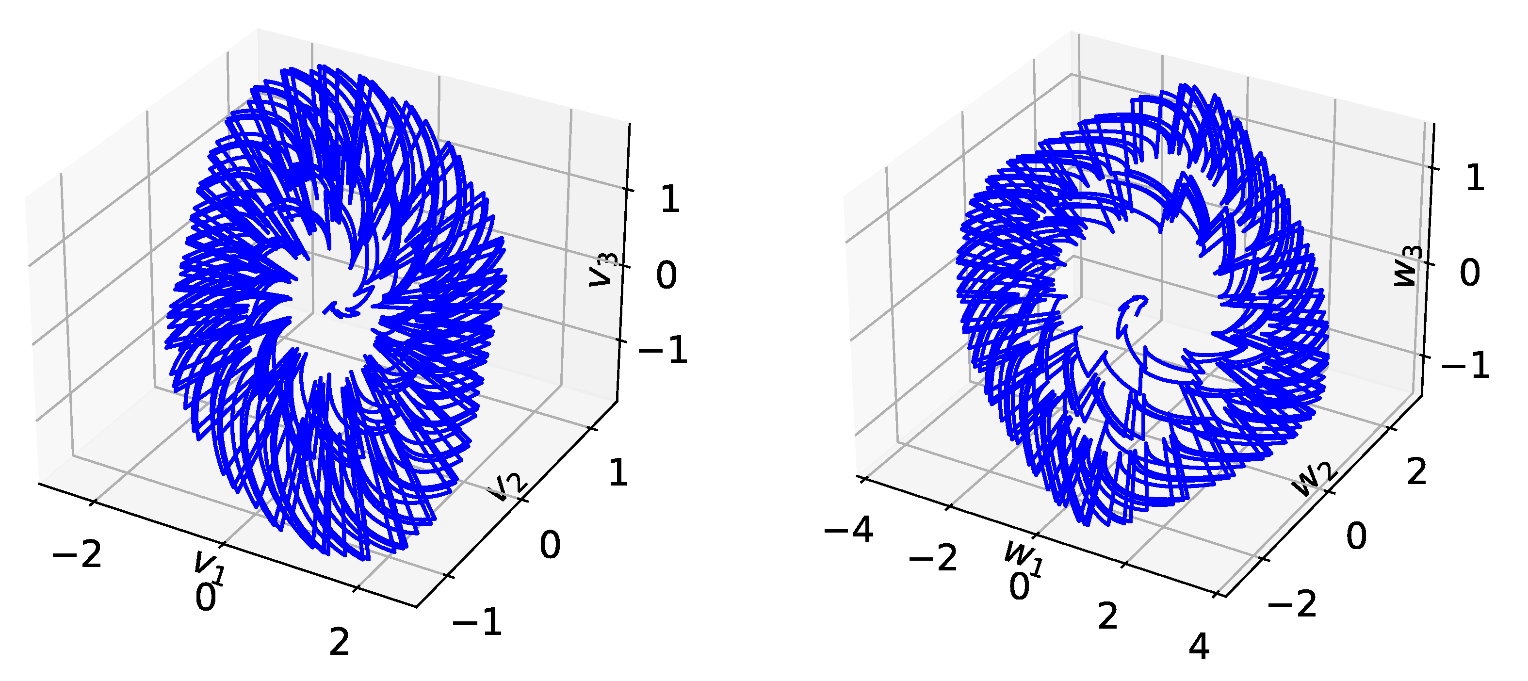
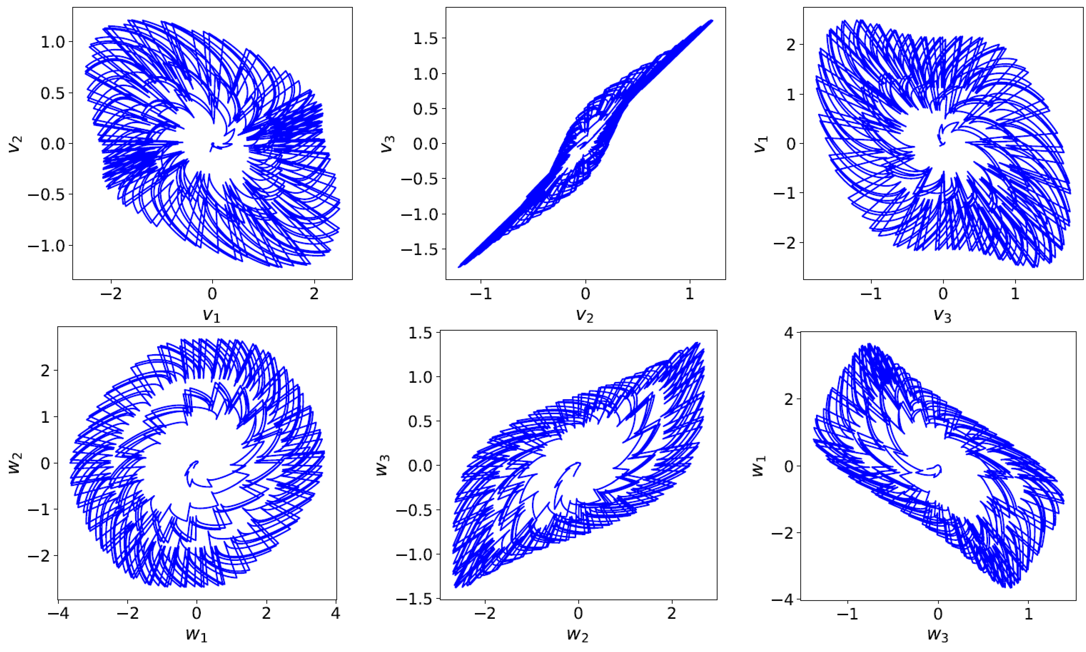
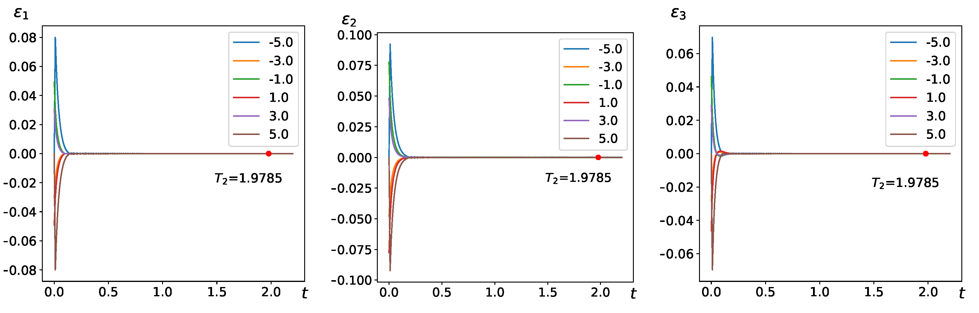
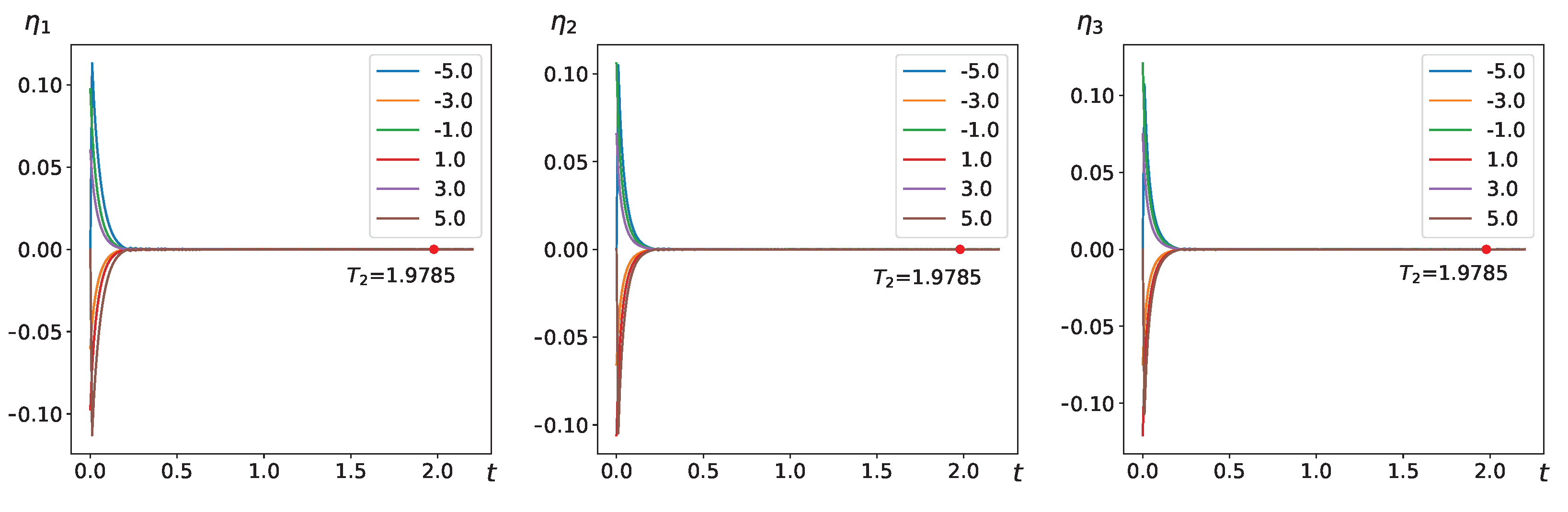
4. Numerical Examples

The simulations are conducted using Python. The $(\alpha -1)$-th-order integrals are computed through the Grünwald–Letnikov method, since, when $\alpha \in (0,1)$, the two fractional-order integrals, Grünwald–Letnikov and Caputo integrals, are indistinguishable in practical applications and completely equivalent [28,40]. To discretize the fractional-order diffusion equation, the L1 approximation method was employed [41]. This section includes two numerical examples to confirm the correctness of the analytical findings presented in the previous section.

Example 1.

Consider the following fractional-order impulsive neural networks with reaction–diffusion term

$$\left\{\begin{array}{ccc}{D}_t^{\alpha }{v}_{\iota }(t,x)=d_{\iota }\Delta v_{\iota }(t,x)-a_{\iota }{v}_{\iota }(t,x)+\sum _{\kappa =1}^3{b}_{\iota \kappa }{h}_{\kappa }(w_{\kappa }(t,x))+I_{\iota },\hfill & \hfill & t\ne t_{\tau },\hfill \\ D_t^{\alpha }{w}_{\kappa }(t,x)={\widehat{d}}_{\kappa }\Delta w_{\kappa }(t,x)-{\widehat{a}}_{\kappa }{w}_{\kappa }(t,x)+\sum _{\iota =1}^3{\widehat{b}}_{\kappa \iota }{\widehat{h}}_{\iota }(v_{\iota }(t,x))+{\widehat{I}}_{\kappa },\hfill & \hfill & t\ne t_{\tau },\hfill \\ v_{\iota }(t_{\tau }^{+},x)={\displaystyle \frac{{\xi }_{\iota }}{\Gamma (2-\alpha )}}{v}_{\iota }(t_{\tau },x),\hfill & \hfill & t=t_{\tau },\hfill \\ w_{\kappa }(t_{\tau }^{+},x)={\displaystyle \frac{{\widehat{\xi }}_{\kappa }}{\Gamma (2-\alpha )}}{w}_{\kappa }(t_{\tau },x),\hfill & \hfill & t=t_{\tau },\hfill \end{array}\right.$$

(24)

for $\iota ,\kappa \in \{1,2,3\}$, and $x\in [-5,5]$, $t\in [0,25]$, the spatial and temporal step sizes are taken as $\Delta x=0.33$ and $\Delta t=0.01$, respectively. We take the parameters to $\alpha =0.9$, $\left\{I_{\iota }\right\}=\left\{{\widehat{I}}_{\kappa }\right\}=0$, $\left\{{\xi }_i\right\}=0.5$ and $\left\{{\overline{\xi }}_j\right\}=0.65$. The other parameters are shown in

Table 1. The main parameters for Example 1.

${\mathit{d}}_{\mathit{\iota }}$	${\widehat{\mathit{d}}}_{\mathit{\kappa }}$	${\mathit{a}}_{\mathit{\iota }}$	${\widehat{\mathit{a}}}_{\mathit{\kappa }}$	${\mathit{b}}_{\mathit{\iota }\mathit{\kappa }}$			${\widehat{\mathit{b}}}_{\mathit{\iota }\mathit{\kappa }}$
0.9631	0.3146	0.0073	1.2633	−2.8999	1.4399	−1.133	−1.9869	2.977	3.0862
0.9631	0.3146	2.6592	0.2561	1.3996	−2.2743	−0.5121	−2.0131	−3.4819	2.2811
0.9631	0.3146	3.0266	1.7172	1.4111	−1.7352	−3.923	−1.2189	−0.1094	−2.8969

. The activation functions are given as $h_{\kappa }(·)=tanh(·)$ and ${\widehat{h}}_{\iota }(·)=tanh(·)$.

The initial conditions are $v_1^0=0.0517sin({\displaystyle \frac{3x}{5}}),v_2^0=0.08146sin({\displaystyle \frac{3x}{5}}),v_3^0=0.04863sin({\displaystyle \frac{3x}{5}})$, $w_1^0=0.10239sin({\displaystyle \frac{3x}{5}})$, $w_2^0=0.11400sin({\displaystyle \frac{3x}{5}})$ and $w_3^0=0.127070sin({\displaystyle \frac{3x}{5}})$. The results presented in Figure 1 and Figure 2, along with the corresponding Lyapunov exponents calculated using the method outlined in Section 2.3 are ${\lambda }_v=(-0.1216,-0.1379,-0.1404)$ and ${\lambda }_w=(-0.1541$, $-0.1374$, $1.376)$. Therefore, the system (24) exhibits a chaotic attractor.

The response system of the system (24) is given as

$$\left\{\begin{array}{ccc}{D}_t^{\alpha }{v}_{\iota }^{*}(t,x)=d_{\iota }\Delta v_{\iota }^{*}(t,x)-a_{\iota }{v}_{\iota }^{*}(t,x)+\sum _{\kappa =1}^m{b}_{\iota \kappa }{h}_{\kappa }(w_{\kappa }^{*}(t,x))+I_{\iota }+u_{\iota }(t,x),\hfill & \hfill & t\ne t_{\tau },\hfill \\ D_t^{\alpha }{w}_{\kappa }^{*}(t,x)={\widehat{d}}_{\kappa }\Delta w_{\kappa }^{*}(t,x)-{\widehat{a}}_{\kappa }{w}_{\kappa }^{*}(t,x)+\sum _{\iota =1}^n{\widehat{b}}_{\kappa \iota }{\widehat{h}}_{\iota }(v_{\iota }^{*}(t,x))+{\widehat{I}}_{\kappa }+{\widehat{u}}_{\kappa }(t,x),\hfill & \hfill & t\ne t_{\tau },\hfill \\ v_{\iota }^{*}(t_{\tau }^{+},x)={\displaystyle \frac{{\xi }_{\iota }}{\Gamma (2-\alpha )}}{v}_{\iota }^{*}(t_{\tau },x),\hfill & \hfill & t=t_{\tau },\hfill \\ w_{\kappa }^{*}(t_{\tau }^{+},x)={\displaystyle \frac{{\widehat{\xi }}_{\kappa }}{\Gamma (2-\alpha )}}{w}_{\kappa }^{*}(t_{\tau },x),\hfill \end{array}\right.$$

(25)

where parameters $d_{\iota }$, ${\widehat{d}}_{\kappa }$, $a_{\iota }$, ${\widehat{a}}_{\kappa }$, $b_{\iota \kappa }$, ${\widehat{b}}_{\kappa \iota }$, $I_{\iota }$, ${\widehat{I}}_{\kappa }$, along with the activations functions $h_{\kappa }(·)$ and ${\widehat{h}}_{\iota }(\dot{)}$, are similar to those in the drive system (24). The jump coefficients ${\xi }_{\iota }=0.5$, ${\widehat{\xi }}_{\kappa }=0.65$. ${\delta }_1={\delta }_2=6.6$, ${\delta }_3=6.4$, ${\widehat{\delta }}_1=6.5,{\widehat{\delta }}_2=6.8,{\widehat{\delta }}_3=6.6$. ${\theta }_1={\theta }_2=3.2$, ${\theta }_3=4.2$, ${\vartheta }_1={\vartheta }_2={\vartheta }_3=3.2$, ${\widehat{\theta }}_1=4.2,{\widehat{\theta }}_2={\widehat{\theta }}_3=3.2$, ${\widehat{\vartheta }}_1={\widehat{\vartheta }}_2=3.2$, ${\vartheta }_3=4.2$, $p=0.4$, $q=1.6$, and ${\widehat{L}}_{\iota }=L_{\kappa }=1.1$, $N_0=0.1$, ${\nu }_{\tau }=0.5$. Consequently, we can easily calculate that

$$\begin{array}{c}\hfill k=max\{\underset{\iota \in \{1,2,3\}}{max}\{-a_{\iota }-{\delta }_{\iota }+{\widehat{L}}_{\iota }\sum _{\kappa =1}^3|{\widehat{b}}_{\kappa \iota }|\},\underset{\kappa \in \{1,2,3\}}{max}\{-{\widehat{a}}_{\kappa }-{\widehat{\delta }}_{\kappa }+L_{\kappa }\sum _{\iota =1}^3|b_{\iota \kappa }|\}\}=-3359.\end{array}$$

This indicates that the inequalities outlined in Theorem 1 are met. Therefore, as shown in Figure 3 and Figure 4, the response system (25) achieves synchronization with the drive system (24) within FXT $T_2=1.9785$ under the controller (7). This confirms the controller’s efficiency in reaching the desired FXT synchronization through numerical means.

Remark 3. 

Figure 1 and Figure 2 clearly show that the system (24) exhibits chaotic phenomena. Fractional-order derivatives consider the entire history of the system; this property can lead to more complex nonlinear phenomena [42]. In impulsive neural networks, the state of the system can change abruptly at a certain moment; therefore, associating the memory of fractional-order derivatives to the abrupt changes of impulsive neural networks can result in a rich variety of dynamical behaviors.

Remark 4. 

Figure 3 and Figure 4 depict the convergence of the error system to zero within the FXT $T_1$, as indicated by Theorem 1. Compared with the works [29,31], the results presented in this paper are more practical and applicable.

As mentioned in the introduction section, there are cases where it is necessary to set the synchronization time in advance. Theorem 2 provided the necessary conditions for PDT synchronization. Now, we validate these conditions numerically, taking into account the PDT synchronization of drive–response systems (24) and (25). All parameters are as previously delineated in the FXT synchronization context. Set the preassigned-time as $T_c=1.9$; then,

$$\begin{array}{cc}\hfill \tilde{k}& =max\{\underset{\iota \in \{1,2,3\}}{max}\{-{\displaystyle \frac{T_0}{T_c}}{a}_{\iota }-{\delta }_{\iota }+{\displaystyle \frac{T_0}{T_c}}{\widehat{L}}_{\iota }\sum _{\kappa =1}^3|{\widehat{b}}_{\kappa \iota }|\},\underset{\kappa \in \{1,2,3\}}{max}\{-{\displaystyle \frac{T_0}{T_c}}{\widehat{a}}_{\kappa }-{\widehat{\delta }}_{\kappa }+{\displaystyle \frac{T_0}{T_c}}{L}_{\kappa }\sum _{\iota =1}^3|b_{\iota \kappa }|\}\}\hfill \\ \hfill & =-1.1623,\hfill \end{array}$$

where $T_0=2.1194$. This ensures that the conditions specified in Theorem 2 are satisfied. Consequently, as demonstrated in Figure 5 and Figure 6, in accordance with Theorem 2, the drive–response systems (24) and (25) achieve synchronization within PDT $T_c=1.9$.

Finally, we examine the impact of the fractional-order parameter $\alpha$ on synchronization by analyzing the outcomes for various values of $\alpha$, such as $\alpha =0.8,0.9,0.95,0.98$.

As observed in Figure 7, the convergence of $\parallel {\epsilon }_i{\parallel }_2$ and ${\parallel \eta \parallel }_2$$(\iota =12,3,\kappa =1,2,3)$ is more rapid for smaller $\alpha$ values. Nonetheless, when $\alpha =0.8$, there is oscillation around $t=0.15$, indicating a transient instability.

To further investigate this behavior, we set $\alpha =0.6$, and Figure 8 reveals more pronounced chattering effects compared to those observed in Figure 7.

5. Conclusions

In this study, the FXT and PDT synchronizations are investigated for the impulsive fractional-order BAM neural networks with diffusion terms. Initially, we presented fundamental knowledge of the fractional-order calculus and the FXT and PDT synchronizations of neural networks. Expanding on prior studies, we integrated the effects of the impulse and fractional-order within reaction–diffusion BAM neural networks. Since, fractional-order calculus and reaction–diffusion processes associated with impulsive BAM neural networks provide a more comprehensive representation of real-world systems. These systems exhibit not only temporal changes but also spatial factors and diffusion effects. Consequently, the scope of applications for BAM neural networks has been broadened in fields such as environmental science and secure communication [43]. We have developed an innovative controller for the system and have formulated adequate conditions for the FXT and PDT synchronizations of drive–response systems, employing the Lyapunov function approach. To substantiate the theoretical results of our proposed model, a numerical example was provided. Nevertheless, stochastic perturbations are frequently inevitable in many dynamical systems. These perturbations enhance the network’s ability to generalize and accurately forecast outcomes in uncertain environments, thus bolstering its robustness and adaptability [34,44,45,46]. In future studies, we will focus on the synchronization of fractional-order BAM neural networks with randomness, thereby enhancing the applicability of our dynamic system.

References

1. Song, C.; Cao, J. Dynamics in fractional-order neural networks. Neurocomputing 2014, 142, 494–948. [Google Scholar] [CrossRef]
2. Chen, J.; Chen, B.; Zeng, Z. Global asymptotic stability and adaptive ultimate mittag-leffler synchronization for a fractional-order complex-valued memristive neural networks with delays. IEEE Trans. Syst. Man Cybern. Syst. 2018, 49, 2519–2535. [Google Scholar] [CrossRef]
3. Zhang, L.; Yang, Y. Bipartite synchronization analysis of fractional order coupled neural networks with hybrid control. Neural Process. Lett. 2020, 52, 1969–1981. [Google Scholar] [CrossRef]
4. Podlubny, I. Geometrical and physical interpretation of fractional integration and fractional differentiation. Fract. Calc. Appl. Anal. 2002, 5, 367–386. [Google Scholar]
5. Luo, R.; Liu, S.; Song, Z.; Zhang, F. Fixed-time control of a class of fractional-order chaotic systems via backstepping method. Chaos Soliton. Fract. 2023, 167, 113076. [Google Scholar] [CrossRef]
6. Balamash, A.S.; Bettayeb, M.; Djennoune, S.; Al-Saggaf, U.M.; Moinuddin, M. Fixed-time terminal synergetic observer for synchronization of fractional-order chaotic systems. Chaos 2020, 30, 073124. [Google Scholar] [CrossRef]
7. He, Y.; Peng, J.; Zheng, S. Fractional-Order Financial System and Fixed-Time Synchronization. Fractal Fract. 2022, 6, 507. [Google Scholar] [CrossRef]
8. Ren, J.; Lei, H.; Song, J. An improved lattice Boltzmann model for variable-order time-fractional generalized Navier–Stokes equations with applications to permeability prediction. Chaos Soliton Fract. 2024, 189, 115616. [Google Scholar]
9. Sun, J.; Zhao, Y.; Li, X.; Wang, S.; Wei, J.; Lu, Y. Fractional Order Spectrum of Cumulant in Edge Detection. In Proceedings of the 2024 IEEE 2nd International Conference on Image Processing and Computer Applications (ICIPCA), Shenyang, China, 28–30 June 2024; pp. 408–412. [Google Scholar]
10. Ding, D.; Jin, F.; Zhang, H.; Yang, Z.; Chen, S.; Zhu, H.; Xu, X.; Liu, X. Fractional-order heterogeneous neuron network based on coupled locally-active memristors and its application in image encryption and hiding. Chaos Soliton Fract. 2024, 187, 115397. [Google Scholar]
11. Chen, L.; Yin, H.; Huang, T.; Yuan, L.; Zheng, S.; Yin, L. Chaos in fractional-order discrete neural networks with application to image encryption. Neural Netw. 2020, 125, 174–184. [Google Scholar] [CrossRef]
12. Wei, T.; Lin, P.; Wang, Y.; Wang, L. Stability of stochastic impulsive reaction–diffusion neural networks with S-type distributed delays and its application to image encryption. Neural Netw. 2019, 116, 35–45. [Google Scholar] [CrossRef] [PubMed]
13. Kowsalya, P.; Kathiresan, S.; Kashkynbayev, A.; Rakkiyappan, R. Fixed-time synchronization of delayed multiple inertial neural network with reaction–diffusion terms under cyber–physical attacks using distributed control and its application to multi-image encryption. Neural Netw. 2024, 180, 106743. [Google Scholar] [CrossRef] [PubMed]
14. Vilas, C.; García, M.R.; Banga, J.R.; Alonso, A.A. Robust feed-back control of travelling waves in a class of reaction–diffusion distributed biological systems. Phys. D Nonlinear Phenom. 2008, 237, 2353–2364. [Google Scholar] [CrossRef]
15. Song, Q.; Cao, J. Global exponential robust stability of cohen-grossberg neural network with time-varying delays and reaction–diffusion terms. J. Frankl. Inst. 2006, 343, 705–719. [Google Scholar] [CrossRef]
16. Cao, J.; Stamov, G.; Stamova, I.; Simeonov, S. Almost periodicity in impulsive fractional-order reaction–diffusion neural networks with time-varying delay. IEEE Trans. Cybern. 2021, 51, 151–161. [Google Scholar] [CrossRef]
17. Ali, M.S.; Hymavathi, M.; Rajchakit, G.; Saroha, S.; Palanisamy, L.; Hammachukiattikul, P. Synchronization of Fractional Order Fuzzy BAM Neural Networks with Time Varying Delays and Reaction Diffusion Terms. IEEE Access 2020, 8, 186551–186571. [Google Scholar] [CrossRef]
18. Lin, J.; Xu, R.; Li, L. Spatio-temporal synchronization of reaction–diffusion BAM neural networks via impulsive pinning control. Neurocomputing 2020, 418, 300–313. [Google Scholar] [CrossRef]
19. Chen, H.; Jiang, M.; Hu, J. Global exponential synchronization of BAM memristive neural networks with mixed delays and reaction–diffusion terms. Commun. Nonlinear Sci. Numer. Simulat. 2024, 137, 108137. [Google Scholar] [CrossRef]
20. Kowsalya, P.; Mohanrasu, S.S.; Kashkynbayev, A.; Gokul, P.; Rakkiyappan, R. Fixed-time synchronization of Inertial Cohen–Grossberg Neural Networks with state dependent delayed impulse control and its application to multi-image encryption. Chaos Soliton. Fract. 2024, 181, 114693. [Google Scholar] [CrossRef]
21. Li, H.; Li, C.; Ouyang, D.; Nguang, S.K. Impulsive synchronization of unbounded delayed inertial neural networks with actuator saturation and sampled-data control and its application to image encryption. IEEE Trans. Neural Netw. Learn. Syst. 2021, 32, 1460–1473. [Google Scholar] [CrossRef]
22. Bishop, S.A.; Eke, K.S.; Okagbue, H.I. Advances on asymptotic stability of impulsive stochastic evolution equations. Comput. Sci. 2021, 16, 99–109. [Google Scholar]
23. Zhang, W.; Li, C.; Huang, T.; He, X. Synchronization of Memristor-Based Coupling Recurrent Neural Networks with Time-Varying Delays and Impulses. IEEE Trans. Neural Netw. Learn. Syst. 2015, 26, 3308–3313. [Google Scholar] [CrossRef] [PubMed]
24. Pratap, A.; Cao, J.; Lim, C.P.; Bagdasar, O. Stability and pinning synchronization analysis of fractional order delayed Cohen–Grossberg neural networks with discontinuous activations. Appl. Math. Comput. 2019, 359, 241–260. [Google Scholar] [CrossRef]
25. Velmurugan, G.; Rakkiyappan, R.; Cao, J. Finite-time synchronization of fractional-order memristor-based neural networks with time delays. Neural Netw. 2016, 73, 36–46. [Google Scholar] [CrossRef] [PubMed]
26. Du, F.; Lu, J. New criterion for finite-time synchronization of fractional order memristor-based neural networks with time delay. Appl. Math. Comput. 2021, 389, 125616. [Google Scholar] [CrossRef]
27. Polyakov, A. Nonlinear feedback design for fixed-time stabilization of linear control systems. IEEE Trans. Automat. Control 2012, 57, 2106–2110. [Google Scholar] [CrossRef]
28. Podlubny, I. Fractional Differential Equations, Mathematics in Science and Engineering; Academic Press: Cambridge, MA, USA, 1999. [Google Scholar]
29. Huang, S.; Xiong, L.; Wang, J.; Li, P.; Wang, Z.; Ma, M. Fixed-time fractional-order sliding mode controller for multimachine power systems. IEEE Trans. Power Syst. 2021, 36, 2866–2876. [Google Scholar] [CrossRef]
30. Xiao, J.; Wen, S.; Yang, X.; Zhong, S. New approach to global Mittag–Leffler synchronization problem of fractional-order quaternion-valued BAM neural networks based on a new inequality. Neural Netw. 2020, 122, 320–337. [Google Scholar] [CrossRef]
31. Khanzadeh, A.; Mohammadzaman, I. Comment on ‘Fractional-order fixed-time nonsingular terminal sliding mode synchronization and control of fractional-order chaotic systems’. Nonlinear Dynam. 2018, 94, 3145–3153. [Google Scholar] [CrossRef]
32. Lee, L.; Liu, Y.; Liang, J.; Cai, X. Finite time stability of nonlinear impulsive systems and its applications in sampled-data systems. ISA Trans. 2015, 57, 172–178. [Google Scholar] [CrossRef]
33. Li, H.; Li, C.; Huang, T.; Ouyang, D. Fixed-time stability and stabilization of impulsive dynamical systems. J. Frankl. Inst. 2017, 354, 8626–8644. [Google Scholar] [CrossRef]
34. Abudusaimaiti, M.; Abdurahman, A.; Jiang, H. Fixed/predefined-time synchronization of fuzzy neural networks with stochastic perturbations. Chaos Solitons Fractals 2022, 154, 111596. [Google Scholar] [CrossRef]
35. Li, H.; Shen, Y.; Han, Y.; Dong, J.; Li, J. Determining Lyapunov exponents of fractional-order systems: A General method based on memory principle. Chaos Solitons Fractals 2023, 168, 113167. [Google Scholar] [CrossRef]
36. Echenausía-Monroy, J.L.; Quezada-Tellez, L.A.; Gilardi-Velázquez, H.E.; Ruíz-Martínez, O.F.; Heras-Sánchez, M.D.C.; Lozano-Rizk, J.E.; Álvarez, J. Beyond chaos in fractional-order systems: Keen insight in the dynamic effects. Fractal Fract. 2024, 9, 22. [Google Scholar] [CrossRef]
37. Sadik, H.; Abdurahman, A.; Tohti, R. Fixed-Time synchronization of reaction–diffusion fuzzy neural networks with stochastic perturbations. Mathematics 2023, 11, 1493. [Google Scholar] [CrossRef]
38. Song, X.; Man, J.; Song, S.; Zhang, Y.; Ning, Z. Finite/fixed-time synchronization for Markovian complex-valued memristive neural networks with reaction–diffusion terms and its application. Neurocomputing 2020, 414, 131–142. [Google Scholar] [CrossRef]
39. Evans, L.C. Partial Differential Equation, 2nd ed.; American Mathematical Society: Providence, RI, USA, 2010. [Google Scholar]
40. Lubich, C. Discretized fractional calculus. SIAM J. Math. Anal. 1986, 17, 704–719. [Google Scholar] [CrossRef]
41. Lin, Y.; Xu, C. Finite difference/spectral approximations for the time-fractional diffusion equation. J. Comput. Phys. 2007, 225, 1533–1552. [Google Scholar] [CrossRef]
42. Huang, C.; Wang, H.; Liu, H.; Cao, J. Bifurcations of a delayed fractional-order BAM neural network via new parameter perturbations. Neural Netw. 2023, 168, 123–142. [Google Scholar] [CrossRef]
43. Wang, Z.; Zhang, W.; Zhang, H.; Chen, H.; Cao, J.; Abdel-Aty, M. Finite-time quasi-projective synchronization of fractional-order reaction–diffusion delayed neural networks. Inform. Sci. 2025, 686, 121365. [Google Scholar] [CrossRef]
44. Abdurahman, A.; Abudusaimaiti, M.; Jiang, H. Fixed/predefined-time lag synchronization of complex-valued BAM neural networks with stochastic perturbations. Appl. Math. Comput. 2023, 444, 127811. [Google Scholar] [CrossRef]
45. Yin, J.; Khoo, S.; Man, Z. Finite-time stability and instability of stochastic nonlinear systems. Automatica 2011, 47, 2671–2677. [Google Scholar] [CrossRef]
46. Torres, J.J.; Muñoz, M.A.; Cortés, J.M.; Mejías, J.F. Special issue on emergent effects in stochastic neural networks with application to learning and information processing. Neurocomputing 2021, 461, 632–634. [Google Scholar] [CrossRef]
Figure 1. The chaotic attractor of v ( t , x ) (left) and w ( t , x ) (right) in system (24), where x = 1 is fixed.
Fractalfract 09 00088 g001
Figure 2. The chaotic attractor of the system (24), where x = 1 is fixed.
Fractalfract 09 00088 g002
Figure 3. The evolution diagram of ε 1 ( t , x ) (left), ε 2 ( t , x ) (middle), and ε 3 ( t , x ) (right).
Fractalfract 09 00088 g003
Figure 4. The evolution diagram of η 1 ( t , x ) (left), η 2 ( t , x ) (middle), and η 3 ( t , x ) (right).
Fractalfract 09 00088 g004
Figure 5. The time evolution diagram of ε 1 ( t , x ) (left), ε 2 ( t , x ) (middle), and ε 3 ( t , x ) (right).
Fractalfract 09 00088 g005
Figure 6. The time evolution diagram of η 1 ( t , x ) (left), η 2 ( t , x ) (middle), and η 3 ( t , x ) (right).
Fractalfract 09 00088 g006
Figure 7. The time evolution diagram of ε ι 2 ( ι { 1 , 2 , 3 } ) and η κ 2 ( κ { 1 , 2 , 3 } ) for α = 0.8 , 0.9 , 0.95 , 0.98 , respectively.
Fractalfract 09 00088 g007
Figure 8. The time evolution diagram of ε ι 2 ( ι { 1 , 2 , 3 } ) (left) and η κ 2 ( κ { 1 , 2 , 3 } ) (right) for α = 0.6 .
Fractalfract 09 00088 g008