Abstract
Amid growing threats of image data leakage and misuse, image encryption has become a critical safeguard for protecting visual information. However, many recent image encryption algorithms remain constrained by trade-offs between security, efficiency, and practicability. To address these challenges, this paper first proposes a novel two-dimensional variable fractional-order coupled quadratic hyperchaotic map (2D-VFCQHM), which incorporates a state-dependent dynamic memory effect, wherein the fractional-order is adaptively determined at each iteration by the mean of the system’s current state. This mechanism substantially enhances the complexity and unpredictability of the underlying chaotic dynamics. Building upon the superior hyperchaotic properties of the 2D-VFCQHM, we further develop a high-performance image encryption algorithm that integrates a novel fusion strategy within a dynamic vector-level diffusion-scrambling framework (IEA-VMFD). Comprehensive security analyses and experimental results demonstrate that the proposed algorithm achieves robust cryptographic performance, including a key space of , inter-pixel correlation coefficients below 0.0018, ciphertext entropy greater than 7.999, and near-ideal plaintext sensitivity. Crucially, the algorithm attains an encryption speed of up to 126.2963 Mbps. The exceptional balance between security strength and computational efficiency underscores the practical viability of our algorithm, rendering it well-suited for modern applications such as telemedicine, instant messaging, and cloud computing.
1. Introduction
Within the landscape of nonlinear dynamics, fractional calculus has emerged as an indispensable tool, endowing mathematical models with the intrinsic memory and hereditary properties characteristic of many real-world phenomena [1,2]. This has been particularly impactful in designing secure cryptosystems, where fractional-order chaotic maps offer demonstrably superior complexity compared to their integer-order counterparts, which are often plagued by vulnerabilities such as narrow chaotic regimes and embedded periodic windows [3]. Yet, the full potential of fractional dynamics is realized by transcending static, fixed-order frameworks [4]. variable-order fractional calculus, particularly where the order is an adaptive function of the system’s own state, introduces a profound level of structural dynamism [5]. By making the system’s memory depth non-static and state-dependent, these models can robustly eliminate periodicity, expand chaotic ranges, and significantly amplify unpredictability. This work capitalizes on this advanced principle, demonstrating how a state-dependent variable-order formulation can induce robust hyperchaotic behavior in an simple coupled quadratic map. The resulting hyperchaotic map serves as the foundation for a novel, high-performance image protection architecture, directly harnessing the principles of adaptive fractional dynamics to meet modern security demands.
With the advancement of information technology, digital images have become an indispensable information carrier, capable of communicating information vividly and rapidly across virtually all sectors, including medical analysis, commercial presentations, and military intelligence [6,7,8]. However, this widespread application creates prominent security and privacy challenges, as unauthorized access to images containing sensitive data can result in significant breaches. Consequently, protecting this sensitive visual information is of paramount importance [9,10]. Unlike text, the inherent properties of image data, namely its large capacity and the high correlation among adjacent pixels, make traditional encryption algorithms like the Advanced Encryption Standard (AES) difficult to apply both securely and efficiently [11,12,13]. As a result, an escalating number of innovative technologies are being utilized to develop novel image encryption algorithms tailored to these unique challenges [14,15,16,17,18,19,20].
Upon continuous and thorough exploration of chaos theory, image encryption leveraging chaotic systems has progressively taken shape as a promising avenue of development within the realm of information security [21,22,23,24]. Chaotic systems exhibit remarkable nonlinear characteristics, including overall stability coupled with local instability, extreme sensitivity to initial conditions, and long-term unpredictability [25,26]. These attributes provide chaotic encryption with unique advantages in the protection of image data [27,28]. In recent years, numerous researchers have been actively engaged in advancing chaotic image encryption technology [17,18,19,29,30,31,32,33,34,35,36].
For instance, Tuli et al. [32] devised an image encryption algorithm that incorporates optimization techniques within a permutation-diffusion framework. While their algorithm’s reliance on classic chaotic maps allows for fast keystream generation, this design choice critically jeopardizes security, as these maps suffer from well-known flaws, including narrow chaotic ranges and uneven state distributions. Lai et al. [33] constructed a hyperchaotic map and developed an encryption algorithm with three rounds of permutation-diffusion operations. Although their chaotic map performs well, its complex structure reduces encryption efficiency. Moreover, relying on a single operation makes their algorithm susceptible to plaintext attacks. Hua et al. [34] introduced a cross-plane encryption algorithm for color images. Their method first blurs the input image for enhanced resistance to plaintext attacks, followed by multi-round permutation-diffusion encryption. However, the blurring uses random values that violate Kerckhoffs’ principle, and the hyperchaotic map employed is excessively complex. Liu et al. [35] suggested a chaotic encryption algorithm leveraging deoxyribonucleic acid (DNA) computing. Its 2-bit encryption mechanism compromises efficiency, and using hash values to initialize the chaotic system introduces complexities in secret key management. Finally, Wang et al. [37] presented an encryption algorithm that exploits a one-dimensional (1D) chaotic map, incorporating a permutation-diffusion framework. To resist plaintext attacks, they directly use the image hash value to initialize the chaotic map, which poses challenges for key management. Furthermore, the map’s limited control parameters severely restrict the effective key space.
Actually, based on our cryptanalysis research, as well as that conducted by other researchers [38,39,40,41], it has been observed that many recent image encryption algorithms still exhibit design deficiencies that impact their practicability, security, and operational efficiency. In light of the aforementioned and other deficiencies in recent encryption algorithms, this paper proposes a novel framework for high-performance image protection grounded in the principles of state-dependent fractional-order dynamics. At the core of our work is a new 2D variable fractional-order coupled quadratic hyperchaotic map (2D-VFCQHM). This hyperchaotic map introduces a state-dependent dynamic memory effect, wherein the fractional-order adaptively updates based on the system’s current state, yielding exceptionally complex and unpredictable dynamics. Exploiting the 2D-VFCQHM, we develop a high-performance image encryption algorithm, termed IEA-VMFD. It features a novel fusion strategy integrated within a dynamic vector-level diffusion-scrambling framework. This framework is specifically designed to overcome the structural limitations of conventional algorithms, achieving superior security and encryption efficiency. The primary contributions of this paper are as follows:
- A novel variable fractional-order hyperchaotic map, termed 2D-VFCQHM, is proposed. Its core innovation lies in the introduction of a state-dependent dynamic memory effect, wherein the fractional-order is adaptively updated according to the current system state. This mechanism significantly enhances the complexity and unpredictability of the map’s chaotic dynamics.
- The chaotic performance of the 2D-VFCQHM is rigorously validated through a comprehensive suite of analyses. These analyses, along with related comparisons, demonstrate that the 2D-VFCQHM exhibits a broader chaotic range and more stable complex dynamics, quantitatively outperforming several recent advanced chaotic maps.
- Building upon the robust dynamics of the 2D-VFCQHM, we propose the IEA-VMFD, a high-performance image encryption algorithm. Its architecture incorporates a novel pixel-fusion preprocessing stage and a dynamic vector-level diffusion-scrambling framework.
- Extensive experiments and comparative analyses prove that the IEA-VMFD is both secure and highly efficient. Key results include a vast key space, excellent plaintext sensitivity, and a fast encryption speed (126.2963 Mbps), demonstrating its practical superiority over other recent algorithms.
The remainder of this paper systematically unfolds our contributions. First, Section 2 introduces the mathematical preliminaries of discrete fractional calculus and presents the 2D-VFCQHM hyperchaotic map, followed by an analysis of its dynamical properties. Next, Section 3 details the architecture of our proposed IEA-VMFD, highlighting its innovative design features. Subsequently, Section 4 subjects IEA-VMFD to a battery of rigorous security and efficiency tests to validate its practical viability and superiority. Finally, Section 5 provides a summary of our work and outlines promising avenues for future research.
2. Proposed 2D-VFCQHM
This section begins by establishing the discrete fractional calculus principles that underpin the construction of the 2D-VFCQHM. Subsequently, a comprehensive analysis validates its key dynamical properties, including fixed points and stability, Lyapunov exponents (LEs), bifurcation and trajectory diagrams, entropy complexity, and statistical randomness, thereby confirming its robust foundation for image encryption.
2.1. Preliminaries of Discrete Fractional Calculus
This section introduces the essential mathematical preliminaries of discrete fractional calculus that underpin the construction of our proposed 2D-VFCQHM. We focus on the Caputo-like delta difference operator, as its definition is well-suited for handling initial value problems in chaotic systems.
The fundamental concept begins with the discrete fractional sum, a concept formalized in the foundational work of Atici and Eloe [1].
Definition 1.
For a function , the v-th order fractional sum starting from a is defined as [1]:
where is the fractional order, , , and is the Gamma function. The term represents the falling factorial function, defined by:
Building on the fractional sum, the Caputo-like fractional difference provides a discrete analogue of the well-known Caputo fractional derivative, and its application to chaotic maps was notably established by Wu and Baleanu [2].
Definition 2.
For a function with and , the v-th order Caputo-like fractional difference is defined as [2,42]:
where is the smallest integer greater than or equal to v, and is the traditional m-th order forward difference operator.
To construct a fractional-order chaotic map, we consider the following discrete fractional initial value problem:
According to the theorem presented in [1], this initial value problem is equivalent to the discrete integral equation:
For the specific application to chaotic maps, we typically set the initial time and consider fractional orders within the range , which implies . Under these standard conditions, the general solution simplifies to the following crucial numerical formula for the fractional-order map [42]:
This discrete fractional sum, which forms the cornerstone of our proposed system, demonstrates that the current state is a weighted sum of all past states from to n. This elegantly embodies the long-term memory effect that distinguishes fractional-order systems from their integer-order counterparts.
2.2. Construction of 2D-VFCQHM
Compared to traditional integer-order chaotic maps, fractional-order chaotic systems, especially those with variable orders, exhibit enhanced complexity and unpredictability owing to their intrinsic memory effects, rendering them highly suitable for cryptographic applications [3,43]. However, many existing fractional-order maps still suffer from notable practical limitations, such as insufficient trajectory ergodicity, limited chaotic parameter ranges, and dynamical instabilities arising from the presence of periodic windows [3,4,5,44]. To address these limitations, we propose the novel variable fractional-order hyperchaotic map called 2D-VFCQHM, the systematic construction of which is detailed as follows.
First, drawing inspiration from the structural simplicity of classical chaotic maps such as the Logistic, Tent, and Sine maps, we begin by constructing a simple yet effective 1D seed map. This map incorporates both a quadratic term and an exponential parameter term to ensure a foundational level of complexity, as described below:
Second, to achieve hyperchaotic behavior, which is characterized by at least two positive LEs and is a desirable property for increasing security, we extend the 1D seed map (Equation (6)) into a 2D coupled system. This is achieved by coupling two identical 1D maps, where the state variable of one equation cross-influences the other. This coupling mechanism enhances the system’s dimensionality and dynamic range. This integer-order system, which serves as the core nonlinear function for our final map, is defined as follows:
The third and most crucial step in our design is to introduce the principles of discrete fractional calculus to impart a memory effect into the system. Building upon the Caputo-like delta difference operator defined in Section 2.1, we integrate a variable fractional-order, , into the map. This fractional-order is not a fixed constant but is adaptively updated at each iteration based on the mean of the previous state variables, . By embedding this state-dependent variable-order fractional sum into the integer-order map (Equation (7)), we arrive at the final formulation of the proposed 2D-VFCQHM:
In Equation (8), is the fractional-order at iteration n, satisfying . The states and are generated from the previous states and , with initial values . The control parameters p and q are positive real numbers.
For the dynamical analysis and image encryption application, we set , , and restrict the control parameters to . This high fractional-order range preserves a strong memory effect, while the chosen parameter region, validated by LE and bifurcation analyses, ensures robust, persistent hyperchaos with excellent ergodicity and no periodic windows. The resulting state-dependent memory mechanism significantly enhances the system’s complexity, unpredictability, and suitability for cryptographic applications, as demonstrated in the following sections.
2.3. Fixed Points and Stability Analysis
A rigorous analytical stability analysis for the proposed system is mathematically intractable. Unlike constant fractional-order systems where stability can be determined by the eigenvalues’ location in the complex plane, the proposed 2D-VFCQHM features a state-dependent variable fractional order , as defined in Equation (8). This implies that the system’s algebraic structure and memory kernel evolve dynamically at every iteration, rendering standard analytical methods inapplicable [4,45]. To provide a theoretical insight into the system’s dynamics, we analyze the fixed points and local stability of its corresponding integer-order limit counterpart (where ), as defined as in Equation (7). This approximation strategy is consistent with methodologies adopted in recent variable-order chaotic system research [5], where fixed points are analyzed via their integer-order equivalents due to the complexity of fractional derivation. While this analysis does not constitute a rigorous stability proof for the fractional-order system, it offers a compelling justification for the absence of stable equilibria, a necessary condition for the emergence of global chaotic dynamics.
A fixed point must satisfy and , leading to the transcendental equations:
By inspection, the origin is a trivial fixed point for all parameter values. As analytical solutions for other non-zero fixed points are infeasible, we conducted an extensive numerical search using a multi-start Newton’s method. For the parameter set , which yields complex hyperchaotic behavior (see Section 2.4 and Section 2.5), we identified 22 additional non-zero fixed points, totaling 23 unique solutions. As expected from the symmetric structure of Equation (7), these points exhibit perfect symmetry about the line .
The local stability of each fixed point is assessed by the eigenvalues of the Jacobian matrix of the integer-order map, where a point is unstable if . The Jacobian matrix is given by:
The stability of all 23 fixed points was analyzed by substituting their coordinates into Equation (10) and computing the corresponding eigenvalues. The results are summarized in Table 1.

Table 1.
Fixed points and stability analysis for the integer-order counterpart.
The analysis reveals that for the parameter set , all 23 fixed points of the integer-order counterpart are unstable, as the maximum magnitude of their eigenvalues is significantly greater than one.
It is crucial to emphasize that the stability analysis presented above applies strictly to the integer-order limit system (Equation (7)). For the proposed state-dependent variable fractional-order system (Equation (8)), a rigorous analytical derivation of stability conditions is mathematically intractable. This is due to the system’s persistent memory effect and the dynamic nature of the fractional order , which updates at every iteration, causing the algebraic structure of the map to evolve continuously. However, the universal instability of all fixed points in the integer-order counterpart serves as a necessary heuristic condition, suggesting that trajectories in the fractional system are continuously repelled from any stationary state. Consequently, to rigorously confirm the hyperchaotic behavior of the actual fractional-order model, we rely on the numerical verification of LEs presented in the following section, which is the standard validation method for variable-order systems where analytical solutions are elusive [5,43,45].
2.4. Hyperchaos Verification via Lyapunov Exponents
Following the heuristic stability analysis, we employ LEs as the definitive numerical metric to characterize the dynamical nature of the proposed 2D-VFCQHM. As widely established in fractional calculus literature [46,47], numerical LEs serve as the standard criterion for confirming chaos and hyperchaos when analytical derivation is mathematically intractable due to variable-order complexity.
The LE is a key quantitative measure of sensitivity to initial conditions in dynamical systems. A positive LE indicates chaotic behavior, while the presence of two or more positive LEs confirms hyperchaotic dynamics [46]. For our proposed 2D-VFCQHM, a rigorous theoretical computation of its LEs is infeasible due to its long-term memory dependence and the state-dependent fractional-order , which varies dynamically with . To obtain a practical estimate of the LE spectrum, we therefore adopt the standard numerical algorithm based on the Jacobian matrix of the local instantaneous map and QR decomposition. This numerical approach is widely recognized and verified in the literature for determining the Lyapunov spectrum of fractional-order systems [5,45,47].
First, the trajectory is generated from the full 2D-VFCQHM model (Equation (8)). Then, along this trajectory, the LEs are computed using the Jacobian matrix of the local instantaneous map, which is defined as the derivative of the nonlinear update functions with respect to the immediate past state. The computation is performed using the classical QR decomposition algorithm [48].
Although this approach constitutes a numerical approximation by neglecting the infinite memory tail, it provides a robust qualitative indication of the system’s sensitivity to initial conditions, grounded in the actual dynamical trajectory. Following this standard methodology, we estimated the two LEs ( and ) across a 2D parameter space where p and q vary from 1 to 5. The resulting LE distributions are shown in Figure 1a,b.
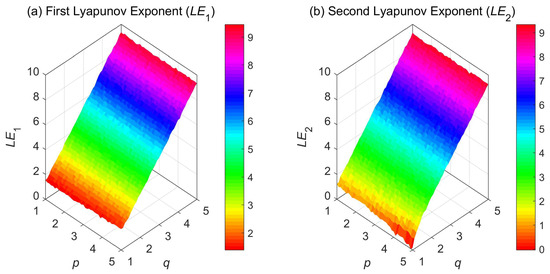
Figure 1.
3D LE plots of 2D-VFCQHM versus control parameters : Left subplot shows , and right subplot shows . The consistently positive values confirm the system’s hyperchaotic state.
Figure 1a shows that remains consistently positive and well above zero across the entire p–q parameter plane, forming a broad plateau region. This indicates that the 2D-VFCQHM exhibits sustained chaotic behavior over a wide range of parameters. More importantly, Figure 1b shows that is also consistently positive throughout the parameter region. The coexistence of two positive LEs provides conclusive numerical evidence of hyperchaotic dynamics, substantiating the heuristic indications from the stability analysis. Thus, the LE analysis confirms that the 2D-VFCQHM exhibits hyperchaotic dynamics over a wide and continuous region of the parameter space. The hyperchaotic nature of the system, characterized by high complexity and sensitivity to initial conditions, renders it a promising candidate for random sequence generation, thereby laying a solid foundation for the subsequent design of our IEA-VMFD.
2.5. Bifurcation and Trajectory Diagrams
In nonlinear dynamics, bifurcation analysis serves as a cornerstone for characterizing system behavior under parameter variation [9]. It involves iteratively computing asymptotic states and plotting them against one or more control parameters to identify parameter regimes associated with fixed points, periodic orbits, or chaos. Figure 2 illustrates the bifurcation characteristics of our 2D-VFCQHM. It includes two sets of 2D bifurcation plots: one varying while fixing , and the other varying with held constant, complemented by 3D bifurcation plots that capture the system’s dynamics when both p and q are simultaneously swept across their respective ranges. A close inspection of these diagrams reveals that the 2D-VFCQHM consistently displays robust chaotic dynamics throughout the entire parameter domain, as evidenced by the dense, uniformly distributed state points across the unit interval. This behavior is quantitatively confirmed to be hyperchaotic by the two positive LEs analyzed in Section 2.4. Such persistent and widespread chaos underscores the map’s strong ergodicity and sensitivity to initial conditions. These are properties that make it especially suitable for cryptographic applications, notably in the field of image encryption.
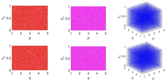
Figure 2.
Bifurcation diagrams of 2D-VFCQHM with control parameters : The first column shows the 2D bifurcation diagrams of versus p (with ) and versus q (with ), respectively. The second column shows the corresponding diagrams for . The third column displays the 3D bifurcation diagrams for and over the entire plane.
To further investigate the dynamical behavior of our 2D-VFCQHM, we present a comprehensive set of trajectory diagrams in Figure 3. These include 2D phase portraits and return maps under fixed system parameters, as well as 3D trajectory evolutions when one of the control parameters is varied. Specifically, the first column displays the classical 2D phase portrait and two return maps ( and ), all computed with , . The second and third columns illustrate the 3D trajectories, respectively, where p and q vary over the interval . The observed trajectories exhibit dense and uniformly distributed patterns across the state space, with no discernible periodic structures or convergence to fixed points. This uniform coverage indicates strong ergodicity and high sensitivity to initial conditions, which are hallmark characteristics of hyperchaotic systems. Notably, the 3D plots reveal intricate spatial dynamics that evolve continuously with changes in the parameters, confirming the system’s complex dynamical structure. This behavior highlights the 2D-VFCQHM’s strong potential as a robust random sequence generator, especially for chaos-driven applications like image encryption.
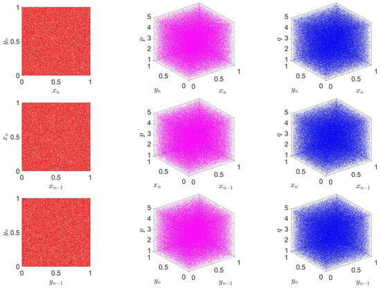
Figure 3.
Trajectory plots of 2D-VFCQHM under different conditions: The first column displays the 2D trajectory plots, including the phase portrait ( versus ) and return maps ( versus and versus ), with fixed parameters (). The second column shows the 3D trajectory evolution as p varies over (with ). The third column shows the corresponding evolution as q varies over (with ).
2.6. Sample Entropy
To quantitatively evaluate the complexity and unpredictability of the sequences generated by chaotic maps, Sample Entropy (SE) is employed as a key performance metric [9]. SE measures the generation rate of new patterns in a time series; a higher SE value indicates greater irregularity and lower predictability, which are highly desirable characteristics for cryptographic systems [49]. Given a time series , the calculation of its SE involves the following steps. First, the series is reconstructed into vectors of dimension m, denoted as . These vectors are defined by the time delay as follows:
The distance between any two vectors is defined as the maximum absolute difference between their corresponding elements. Then, for a given tolerance radius r, let be the number of vectors whose distance from is less than or equal to r. The average probability for dimension m is calculated as:
Similarly, the dimension is increased to to obtain . The SE is then defined as:
In our comparative experiment, to rigorously evaluate the complexity advantage of the proposed system, we selected five representative chaotic maps from recent high-impact literature as benchmarks. These maps were carefully chosen to cover the evolution of chaotic map design across three distinct categories:
- Variable Fractional-Order Map: VFSM [5], representing the state of the art 1D systems where the order varies with time;
- Constant Fractional-Order Maps: 2D-FOCM [44] and NTDM [4], representing standard discrete fractional maps with fixed memory kernels;
- Conventional Integer-Order Maps: 2D-SCMCI [50] and 2D-LCCCM [51], representing high-performance integer-order hyperchaotic systems.
This selection allows for a comprehensive assessment: comparing against integer-order maps highlights the value of the fractional memory effect, while comparing against constant and 1D variable fractional maps demonstrates the superiority of our proposed 2D state-dependent variable-order mechanism.
For a fair comparison, the ranges of variable control parameters for all maps are kept consistent. We specifically selected benchmark maps that possess a primary control parameter capable of supporting the common numerical range of . This compatibility eliminates the need for parameter normalization or scaling. Specifically, we varied parameter a for VFSM, NTDM, and 2D-SCMCI, and parameter for 2D-FOCM and 2D-LCCCM. All other system parameters were fixed at the preferred values reported in their respective literature [4,5,44,50,51]. For the proposed 2D-VFCQHM, the parameter p is varied within (with ). The resolution for all parameter sweeps is set to 100 points. The system is first iterated for 1000 steps to eliminate transient effects. Then, a sequence of 2000 points is generated for analysis. The adopted SE calculation parameters are embedding dimension , time delay , and tolerance radius , where std is the standard deviation of the generated sequence.
Figure 4 presents the comparative results () of all six maps. As illustrated, our 2D-VFCQHM (red curve) consistently exhibits the highest SE values across the entire parameter range, maintaining a stable and high level of complexity. In contrast, the benchmark maps show varying degrees of inferiority. The constant fractional-order map (2D-FOCM) and integer-order map (2D-SCMCI) exhibit highly unstable performance, with their SE values frequently dropping to near zero, indicating the presence of periodic windows. While the 1D variable-order map (VFSM) and other benchmarks (NTDM, 2D-LCCCM) show relatively better performance, their SE values are consistently lower than that of the proposed 2D-VFCQHM. This confirms that the state-dependent variable order combined with a 2D coupled structure significantly amplifies the system’s unpredictability beyond existing methods.
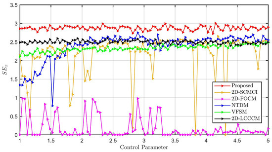
Figure 4.
Superior hyperchaotic complexity of 2D-VFCQHM demonstrated by comparison: Across the entire tested parameter range, our 2D-VFCQHM maintains a significantly higher and more stable entropy level than the five benchmark maps.
2.7. Kolmogorov-Sinai Entropy
Kolmogorov-Sinai entropy (KE) is a fundamental measure of chaos in dynamical systems, quantifying the rate of information generation, or equivalently the loss of predictability, along trajectories. A positive KE confirms chaotic behavior, and higher values indicate stronger unpredictability, which is essential for cryptographic applications to resist prediction-based attacks [52]. To robustly evaluate the chaotic performance of the proposed 2D-VFCQHM, we employ the widely recognized Grassberger-Procaccia algorithm to estimate its KE [53]. The KE is derived from the correlation integral , which calculates the probability that two points in the reconstructed phase space are within a distance r. For a time series of length N, the correlation integral for an embedding dimension m is given by:
where and are vectors in the m-dimensional phase space, and is the Heaviside step function. The KE is then estimated as the limit:
To ensure a fair and direct comparison with the SE analysis, we evaluate the of the proposed 2D-VFCQHM against the same set of five benchmark chaotic maps categorized in Section 2.6 (VFSM, 2D-FOCM, NTDM, 2D-SCMCI, and 2D-LCCCM). All experimental parameters were held consistent with the previous section.
Figure 5 presents the corresponding results. Like the SE analysis, the 2D-VFCQHM consistently achieves the highest and most stable KE values. In contrast, the conventional integer-order and constant fractional-order benchmarks exhibit significant fluctuations and frequent transitions into periodic regimes (near-zero KE values). These results further support the SE analysis, reinforcing that the state-dependent variable-order mechanism confers superior hyperchaotic complexity compared to both constant-order and integer-order counterparts.
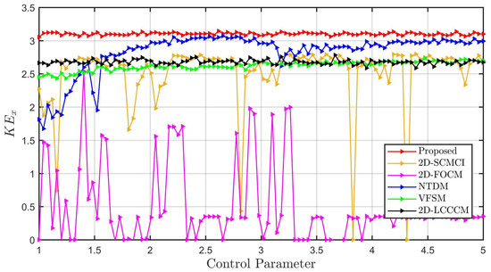
Figure 5.
Outstanding hyperchaotic performance of 2D-VFCQHM demonstrated by comparison: Across the entire tested parameter range, our 2D-VFCQHM achieves consistently higher and more stable entropy compared to five benchmark chaotic maps.
2.8. Randomness Test
The NIST SP 800-22 test suite constitutes a rigorous and widely accepted benchmark for evaluating the statistical randomness of binary sequences [12]. It is specifically designed to detect non-randomness, thereby certifying the suitability of random number generators for secure applications [48]. Accordingly, we subject the hyperchaotic sequences of our 2D-VFCQHM to the NIST SP 800-22 battery, verifying their randomness and establishing their viability for image encryption.
For our experimental setup, the parameters of the 2D-VFCQHM are set to and . The initial conditions and are initialized with MATLAB’s rand() function to enhance the generality of experimental results. The resulting hyperchaotic sequences from the x- and y-components are then converted into binary sequences of length bits, in accordance with the NIST SP 800-22 requirements. This procedure is repeated 20 times to produce 40 binary sequences, enabling comprehensive statistical evaluation.
According to the NIST SP 800-22 evaluation criteria, a test is considered passed if the computed p-value is ≥0.01 [12]. Our final results indicate that all 40 generated binary sequences, 20 from the x-component and 20 from the y-component, successfully passed all statistical tests, with all p-values exceeding 0.01. This demonstrates that the 2D-VFCQHM generates sequences exhibiting high-quality randomness suitable for cryptographic applications. A representative set of test results for one pair of x and y sequences is presented in Table 2.

Table 2.
NIST SP 800-22 evaluation results of 2D-VFCQHM.
3. Proposed IEA-VMFD
Leveraging the exceptional hyperchaotic properties of the 2D-VFCQHM, we have further devised an efficient image encryption algorithm termed IEA-VMFD, aiming to provide robust protection for image data. Our IEA-VMFD comprises a series of meticulously crafted encryption steps: generating plaintext-related parameters, generating keystreams, image preprocessing, dynamic dual-vector diffusion, and interlaced vector-level scrambling. As depicted in Figure 6, dynamic dual-vector diffusion and interlaced vector-level scrambling will be executed twice, resulting in a novel diffusion-scrambling mechanism that deviates from common permutation-diffusion designs.
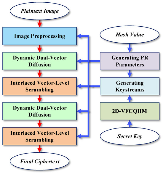
Figure 6.
Enryption process of IEA-VMFD.
3.1. Generating Plaintext-Related Parameters
The independence of the encryption process from the plaintext is a critical vulnerability that makes numerous recent algorithms susceptible to cryptanalysis [38,41]. To address this, our proposed IEA-VMFD algorithm incorporates plaintext-related parameters into the encryption process to enhance its resilience against plaintext attacks. For the input pixel matrix , derived from one color image or three grayscale images, its plaintext-related parameters can be produced as follows:
- Step 1: Utilize the SHA-256 hash function, which is highly sensitive to the input plaintext, to obtain a 256-bit hash value of .
- Step 2: Transform the hash value into a byte vector of size .
- Step 3: Generate four new bytes () with :
- Step 4: Append the generated four bytes () to the end of , making it a byte vector containing 36 bytes.
- Step 5: Perform multiplication, summation, and XOR operations on the 36 bytes within , ultimately deriving two plaintext-related parameters and :where () are six temporary variables, prod(•) denotes the sequential multiplication of the input operands one by one, and ⊕ represents a bitwise XOR operation.
3.2. Generating Keystreams
In our IEA-VMFD, the generation of keystreams involves two phases. Initially, once the secret key is agreed upon, a sufficiently long chaotic sequence can be pre-generated before initiating the encryption process. Secondly, during the encryption process of a specific image, this initial chaotic sequence is further converted into the required keystreams.
Assuming the size of the largest image is , the 2D-VFCQHM utilizes the first six components of (from to ) to produce a chaotic sequence of length . Here, the number 1536 corresponds to the quantity of chaotic values that are discarded. Specifically, 512 of these are discarded under the control of the last key component , while 1024 are discarded based on the plaintext-related parameters and .
During the encryption of a particular image of size , IEA-VMFD converts the pre-generated sequence into three keystreams, , and , for subsequent encryption steps. Since and always hold, the pre-generated sequence is always long enough when encrypting different images, eliminating the need to regenerate chaotic sequences. This approach, unlike algorithms that use hash values directly as secret keys, enhances the encryption efficiency and practicality of our IEA-VMFD. The specific conversion process for generating , , and from is as follows:
- Step 1: The first to be obtained is , which will be used for image preprocessing and two rounds of dynamic dual-vector diffusion:where the value of is contingent upon both the key component and two plaintext-related parameters and , specifically, .
- Step 2: Next, the keystream is obtained, which will be used for the first round of interleaved vector-level scrambling:where returns an integer value which is less than or equal to its operand.
- Step 3: Lastly, is generated, which will be utilized for the second round of interleaved vector-level scrambling:
3.3. Image Preprocessing
Prior to conducting the subsequent two rounds of diffusion-scrambling operations, we initially preprocess the input image to reduce the computational burden of subsequent encryption steps. Specifically, we first reshape the input pixel matrix into a 1D pixel vector and perform a sorting permutation based on logical segmentation. The permuted 1D pixel vector is then converted into an form to facilitate the pixel fusion operation. Ultimately, the pixel matrix is fused into a 2D pixel matrix of size . Specifically, the pixel preprocessing of IEA-VMFD is executed as Algorithm 1.
| Algorithm 1 Image preprocessing of IEA-VMFD. |
|
3.4. Dynamic Dual-Vector Diffusion
The majority of chaotic image encryption algorithms employ a permutation-diffusion framework. However, the requirement for reversibility often makes the final diffusion stage in such frameworks vulnerable to cryptanalysis through arithmetic inversion [38,41]. Therefore, our proposed IEA-VMFD introduces a novel diffusion-scrambling architecture where the diffusion stage precedes the scrambling stage.
Furthermore, to enhance the key sensitivity and plaintext sensitivity of the encryption process, we have simultaneously introduced one chaotic value and two plaintext-related parameters and into the designed dynamic dual-vector diffusion. Specifically, before carrying out the vector-level diffusion operation, we first execute a dynamic logical partitioning which is contingent upon the chosen chaotic value , along with and , as outlined in Algorithm 2.
| Algorithm 2 Dynamic dual-vector diffusion of IEA-VMFD. |
|
3.5. Interlaced Vector-Level Scrambling
Permutation, commonly known as scrambling, is a fundamental building block for robust image encryption algorithms [52,54]. Its primary function is to rearrange pixel positions, a process that shatters the strong native correlations between adjacent pixels and renders the image’s visual content unrecognizable. As stated in Section 3.4, we employ a post-applied scrambling operation to bolster the protection of the diffusion operation, shielding it from arithmetic inversion. Furthermore, we employ vector-level scrambling operations to enhance the attainment of high encryption efficiency. Meanwhile, to optimize the scrambling outcome, we have devised an interleaved scrambling approach, as detailed in Algorithm 3.
| Algorithm 3 Interlaced vector-level scrambling of IEA-VMFD. |
|
Our interlaced vector-level scrambling consists of two phases: odd-column scrambling and even-column scrambling. Initially, during the odd-column scrambling phase, the number of even- and odd-columns within the image is determined. Following this, the scrambling index vector for the odd columns is derived by sorting chaotic values. Ultimately, once the column index vector for the odd-columns is determined, the odd-columns undergo scrambling and XOR substitution based on the scrambling index vector. The scrambling method for the even-columns is essentially the same as that for the odd-columns. The sole distinction is that, during the scrambling of the even-columns, a modular addition substitution is concurrently executed, rather than an XOR substitution.
The encryption process, illustrated in Figure 6, is designed to operate on either a single color image or three grayscale images. Following an initial preprocessing stage, the data is subjected to two iterations of a diffusion-scrambling block, which ultimately yields the final ciphertext. Upon receiving the ciphertext and the plaintext hash value, the decryptor can reconstruct the original input by following the decryption process outlined in Figure 7. As this process is the exact inverse of the encryption procedure, its steps are omitted for brevity.
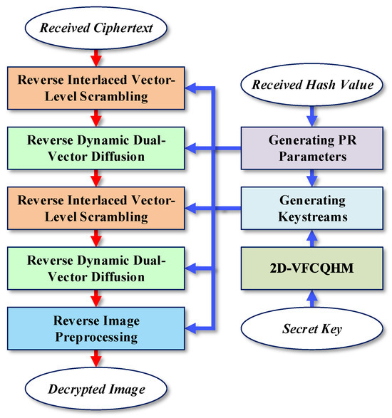
Figure 7.
Decryption process of IEA-VMFD.
4. Experiments and Analyses
To validate the performance of the proposed IEA-VMFD, a series of experiments were conducted to assess its security features and encryption efficiency. The experimental platform was MATLAB R2017a, running on a computer equipped with an Intel Xeon E3-1234 v3 processor (@ 3.40 GHz) and 8 GB of RAM. The images used for testing are from the well-known USC-SIPI database (https://sipi.usc.edu/database/, accessed on 16 September 2025). For each experiment, secret keys were randomly selected from the key space to ensure the generality of the results.
4.1. Visual Effect
An effective image encryption algorithm must ensure visual security [34]. The encrypted image should appear as unintelligible, noise-like data, revealing no information about the original plaintext. Conversely, decryption with the correct key must losslessly reconstruct the original image.
We encrypted and decrypted six standard test images of varying sizes and styles. As shown in Figure 8, the encrypted images exhibit uniform noise-like patterns with no discernible structures, while the decrypted images are visually identical to the originals. This confirms that IEA-VMFD is lossless and fully invertible, providing strong visual security without introducing distortion.
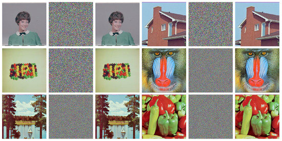
Figure 8.
Visual effect evaluation for IEA-VMFD: The first and fourth columns present six test images (4.1.03, 4.1.05, 4.1.07, 4.2.03, 4.2.06, and 4.2.07); the second and fifth columns depict the corresponding encrypted ones; and the third and sixth columns showcase the decrypted ones.
4.2. Key Space
The resilience of an image encryption algorithm against brute-force attacks hinges heavily on the size of its key space. A vast key space poses an insurmountable challenge for attackers attempting to find the correct secret key through exhaustive search [52]. In the current research landscape, it is widely acknowledged that a secure encryption algorithm must have a key space [12,55]. As described in Section 3.2, the secret key of our IEA-VMFD comprises seven components: , , p, q, , , and . Among these components, the initial conditions and are defined in the open interval with a numerical precision of . The parameters p and q are selected from the closed interval , also with a precision of . The control parameters and are constrained to the intervals and , respectively, each with a precision of . The final component, , is an integer selected from . Therefore, the total key space size of IEA-VMFD, denoted as , is the product of the possible values for each component:
Given that significantly exceeds the generally required , it is reasonable to conclude that our IEA-VMFD can effectively withstand brute-force attacks.
4.3. Key Sensitivity
Key sensitivity is a fundamental security requirement for any robust encryption algorithm. A highly sensitive algorithm ensures that any slight modification to the secret key results in a drastically different ciphertext [54]. This behavior effectively resists differential cryptanalysis, a common threat to encryption systems. The key sensitivity of the IEA-VMFD is shown in Figure 9. Specifically, we began by generating a random secret key:
Subsequently, we made minimal adjustments to each component of , resulting in seven new keys. Finally, we used them to encrypt the identical image (4.2.05) and conducted a comparative analysis of the eight resulting ciphertext images. As shown in Figure 9, all ciphertext images appear as unintelligible noise, effectively obscuring the plaintext’s visual content. The seven difference images demonstrate that a minimal change in any single key component leads to a significant and random-like transformation of the entire ciphertext. This result confirms that the IEA-VMFD possesses high key sensitivity, making it highly resilient to differential attacks.
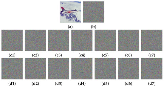
Figure 9.
Key sensitivity test outcomes for IEA-VMFD: (a) 4.2.05; (b) ciphertext of (a); (c1) ciphertext generated by ; (c2) ; (c3) ; (c4) ; (c5) ; (c6) ; (c7) ; (d1) difference for (b,c1); (d2) difference for (b,c2); (d3) difference for (b,c3); (d4) difference for (b,c4); (d5) difference for (b,c5); (d6) difference for (b,c6); (d7) difference for (b,c7).
4.4. Differential Attacks
Differential attacks exploit how small changes in plaintext affect the ciphertext to deduce information about the key or algorithm. A robust encryption algorithm must therefore exhibit high sensitivity to plaintext variations [41]. To assess this property in IEA-VMFD, we created two modified versions of the plaintext image (4.2.07) by altering a single bit in each, as shown in Figure 10(a2,a3). These images were then encrypted, and their difference images were computed against the original ciphertext. As illustrated in Figure 10, both the ciphertexts and the difference images are uniformly noise-like. This result confirms that even a one-bit change in the plaintext causes a complete and unpredictable change in the ciphertext, demonstrating the algorithm’s strong resistance to differential attacks.
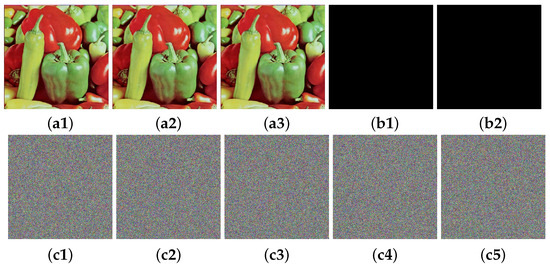
Figure 10.
Visual presentation of IEA-VMFD’s sensitivity to single-bit changes: (a1) 4.2.07; (a2) single-bit at (3,5,1) was changed; (a3) single-bit at (498,499,3) was changed; (b1) difference for (a1,a2); (b2) difference for (a1,a3); (c1) ciphertext of (a1); (c2) ciphertext of (a2); (c3) ciphertext of (a3); (c4) difference for (c1,c2); (c5) difference for (c1,c3).
For a more accurate verification of IEA-VMFD’s plaintext sensitivity, we conducted relevant quantitative assessments, employing two common metrics that quantify plaintext sensitivity [6]. The first metric, known as the normalized pixel change rate (NPCR), quantifies the percentage of pixels that vary between two images. The second, called the unified average changing intensity (UACI), evaluates the average degree of pixel alteration. For two images, and , each of size , one can quantify the differences between them via the mathematical definitions below:
where indicates the difference between the two pixels located at . When the pixel values differ, is set to 1; otherwise, is set to 0. The calculated NPCR and UACI values are presented in Table 3 and Table 4, respectively. For each test, a single, randomly selected pixel in the plaintext image was altered. The results show that the average NPCR and UACI scores for IEA-VMFD are extremely close to the theoretical ideal values of 99.6094% and 33.4635%. Furthermore, when compared with four recent algorithms, the proposed IEA-VMFD not only achieves average scores nearer to the ideal but also exhibits lower variance, indicating greater stability. These quantitative results confirm the algorithm’s high sensitivity to plaintext variations.

Table 3.
Comparison of NPCR results (%) for different algorithms.

Table 4.
Comparison of UACI results (%) for different algorithms.
4.5. Pixel Distribution
Pixel distribution analysis is a key test for evaluating an encryption algorithm’s resistance to statistical attacks [54]. As shown in Figure 11, the plaintext’s pixel distribution is highly irregular, revealing its statistical characteristics. In contrast, the pixel distribution of the corresponding ciphertext produced by IEA-VMFD is nearly uniform, indicating that the pixel values are evenly distributed. This uniformity conceals the statistical profile of the original image, thus confirming the IEA-VMFD’s effectiveness in preventing attacks that exploit pixel distribution patterns.
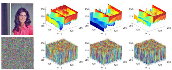
Figure 11.
3D visual exhibitions of pixel distribution for IEA-VMFD: The upper row presents the input image 4.1.04, along with 3D pixel distribution exhibitions for its red, green, and blue channels; and the lower row showcases the encrypted image, accompanied by 3D pixel distribution exhibitions.
To further evaluate the distribution uniformity of the ciphertext pixels in the images produced by IEA-VMFD, we conducted a chi-square test. For 8-bit images, the chi-square values can be computed with the following equation:
where is the number of pixels with the value of , and R and C correspond to the number of rows and the number of columns in an image, respectively. At a significance level of 0.05, the chi-square distribution yields a critical value of 293.2478. An encrypted image is deemed to have passed the chi-square test if its calculated chi-square value falls below this threshold [58]. We computed the chi-square values for three encrypted images produced by IEA-VMFD, as presented in Table 5. All the chi-square values obtained are notably smaller than 293.2478, revealing that the ciphertext pixels output by IEA-VMFD exhibit a high degree of uniformity. This uniformity, in turn, fortifies the resistance of IEA-VMFD against attacks targeting pixel distribution.

Table 5.
Chi-square test results for IEA-VMFD.
4.6. Pixel Correlation
Adjacent pixels in plaintext images are typically highly correlated, which can be a security vulnerability. An effective encryption algorithm must therefore decorrelate these pixels to resist statistical attacks [34]. To evaluate this, we analyzed the pixel correlations in image 4.1.07 before and after encryption. As shown in Figure 12, the plaintext image exhibits strong linear correlations in all directions. In contrast, the pixel distribution in the ciphertext image is random and uniform. This demonstrates our proposed IEA-VMFD’s effectiveness in eliminating pixel correlations.
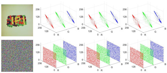
Figure 12.
Correlation analysis of adjacent pixels for IEA-VMFD: The first row shows the plaintext image and its correlation plots for the horizontal, vertical, and diagonal directions. The second row displays the corresponding ciphertext and its correlation plots.
Additionally, we quantitatively analyzed the pixel correlation in three encrypted images using the Correlation Coefficient (CC). The CC value can be computed by applying the mathematical definition:
where and represent pixel values. and denote expectations, and and represent variances. The CC values for the plaintext and ciphertext images are listed in Table 6. As the data shows, the correlation coefficients of the plaintext image are high (>0.7) in all directions. After encryption with IEA-VMFD, these coefficients are reduced to very low values (<0.0018). This confirms that IEA-VMFD effectively decorrelates adjacent pixels, strengthening its resistance to statistical attacks.

Table 6.
CC values for three original and encrypted images.
4.7. Information Entropy
In image encryption, information entropy is a key metric for evaluating ciphertext quality, as it quantifies the randomness of the ciphertext pixels [54]. Formally, the entropy of an 8-bit image is given by the following definition:
where N is the number of pixel values , and is the probability of . A higher information entropy value in a ciphertext signifies greater randomness and a more uniform pixel distribution, which are characteristic of a strong encryption algorithm. For an 8-bit image, the ideal entropy is 8. We encrypted four test images with IEA-VMFD and calculated the entropy for the original and encrypted versions. The results in Table 7 show that the entropy of each ciphertext is significantly higher than that of the corresponding plaintext and consistently close to the ideal value of 8. This confirms the effectiveness of IEA-VMFD in producing ciphertexts with a nearly ideal random distribution.

Table 7.
Information entropy of four input images and their ciphertext images.
Additionally, a comparative analysis of information entropy was conducted against five recent algorithms (Table 8). The results show that the ciphertext produced by IEA-VMFD achieves the highest entropy score among all compared algorithms. This suggests that the IEA-VMFD offers superior performance in terms of ciphertext randomness and uniformity.

Table 8.
Entropy scores for IEA-VMFD and five competing algorithms.
4.8. Robustness Analysis
During the processes of transmission and storage, ciphertext pixels are susceptible to loss or damage. Therefore, a resilient encryption algorithm must be able to tolerate a certain level of pixel degradation [56]. To assess the robustness of IEA-VMFD, we performed a series of simulation experiments on the encrypted images it produces.
To simulate noise attacks, we added salt-and-pepper noise at five different densities (0.01, 0.03, 0.05, 0.07, and 0.09) to the ciphertext of image 4.2.07. The noisy ciphertexts are displayed in the first row of Figure 13 and were then decrypted. As the decrypted results show, the image remains visually clear at lower noise densities (<0.05). Although image quality degrades as the noise density increases, the main visual content remains recognizable even at the highest level of 0.09. This demonstrates the IEA-VMFD’s strong robustness against noise attacks.
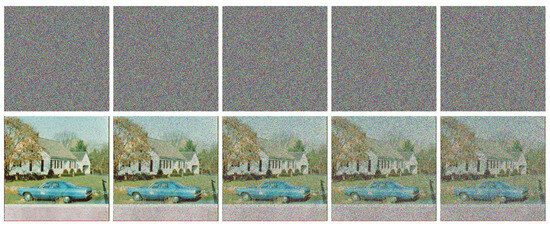
Figure 13.
Robustness of IEA-VMFD against noise attacks: The first row shows the ciphertext images corrupted by noise at various densities (0.01, 0.03, 0.05, 0.07, and 0.09). The second row displays the corresponding decrypted images.
Similarly, we simulated data loss attacks by cropping various sections from the ciphertext of image 4.2.03. The cropped ciphertexts and their corresponding decrypted images are shown in the first and second rows of Figure 14, respectively. As expected, the decrypted image quality degrades as the amount of data loss increases. However, even with a substantial loss of data (e.g., four blocks), the main visual content of the original image remains largely recognizable. This result demonstrates that the IEA-VMFD possesses strong robustness against data loss attacks.
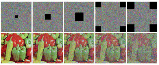
Figure 14.
Robustness of IEA-VMFD against data loss attacks: The first row shows ciphertexts with various sections removed (, , , , and ). The second row displays the corresponding decrypted images.
4.9. Efficiency Analysis
Given the immense data volume and high transmission rates characteristic of modern image communications, encryption efficiency is paramount for practical applications such as telemedicine and cloud computing [55,56]. For an input image of size , any encryption algorithm inevitably possesses a computational complexity of . Therefore, the key to high performance lies in minimizing the computational overhead per pixel.
To demonstrate the exceptional efficiency of our IEA-VMFD, comparative experiments were conducted on a computer equipped with an Intel Xeon E3-1234 v3 CPU @ 3.40 GHz and 8 GB RAM, running MATLAB R2017a. To ensure reliability, the reported processing times are calculated as the average of 100 encryption cycles. It is worth emphasizing that the high encryption speed (low latency) achieved by IEA-VMFD is attributed to three core structural optimizations designed to overcome traditional bottlenecks:
- Reusable Chaotic Sequence: Unlike schemes that regenerate chaotic sequences for every image based on hash values, our design allows the base chaotic sequence to be generated once upon key initialization and reused, significantly reducing computational overhead.
- Data Volume Reduction: The image preprocessing stage (Section 3.3) fuses the RGB layers, reducing the matrix dimension from to . This 6-fold reduction in data volume drastically lowers the computational load for subsequent stages.
- Vector-Level Architecture: As detailed in Section 3.4 and Section 3.5, both diffusion and scrambling operations are performed on full vectors (rows/columns). This avoids slow pixel-wise loops and fully exploits the matrix operation capabilities of the testing environment.
As demonstrated in Table 9 and Table 10, we compared IEA-VMFD with five recently published encryption algorithms. Across three prevalent input scales, the IEA-VMFD demonstrated remarkable superiority. For color images of size , the IEA-VMFD required an average of only 0.2388 s to complete encryption. Additionally, the IEA-VMFD achieved an average rate of 126.2963 Mbps, which is sufficient for various applications such as telemedicine, instant messaging, and cloud computing.

Table 9.
Average time overheads (Seconds) of IEA-VMFD and five other algorithms.

Table 10.
Average rates (Mbps) of IEA-VMFD and five other algorithms.
5. Conclusions
In this paper, we addressed the persistent challenge of balancing security, efficiency, and practicability in modern image encryption. We introduced a novel 2D hyperchaotic map and developed a corresponding high-performance cryptographic algorithm, both deeply rooted in the principles of state-dependent fractional-order dynamics.
The cornerstone of our work is the new 2D variable fractional-order hyperchaotic map called 2D-VFCQHM. By architecting a state-dependent mechanism where the fractional-order adaptively evolves based on the system’s current state, the 2D-VFCQHM transcends the limitations of conventional integer-order and fixed-order fractional maps. A comprehensive suite of dynamical analyses confirmed its superiority; it exhibits a broad, continuous hyperchaotic regime free of periodic windows, as evidenced by two consistently positive LEs. Furthermore, comparative evaluations of SE and KE revealed that our map generates sequences of significantly higher complexity and unpredictability than several recent chaotic maps. Rigorous NIST SP 800-22 tests further validated the excellent statistical randomness of its output, establishing it as a robust foundation for cryptographic applications.
Building upon this robust hyperchaotic foundation, we designed and implemented a novel high-performance image encryption algorithm termed IEA-VMFD. Its architecture synergistically combines several innovations, including a pixel-fusion preprocessing stage and a dynamic vector-level diffusion-scrambling framework, engineered to enhance security while maximizing encryption throughput. Extensive experimental results demonstrated the algorithm’s exceptional performance. It provides robust security, featuring a vast key space of approximately , near-ideal plaintext sensitivity (average NPCR of 99.6096% and UACI of 33.4637%), and strong resilience against statistical and differential attacks. Crucially, the IEA-VMFD achieves an outstanding encryption speed of up to 126.2963 Mbps, significantly outperforming many recent algorithms. This superior balance between cryptographic strength and practical efficiency makes our algorithm highly suitable for demanding, real-world applications such as telemedicine, cloud computing, and secure instant messaging.
While the proposed IEA-VMFD exhibits superior cryptographic performance, it is important to acknowledge certain limitations. Specifically, the decryption process relies strictly on the integrity of the received SHA-256 hash, lacking explicit error-correction protocols to handle channel noise or malicious tampering. Furthermore, the current framework is optimized for single-image processing, which restricts its efficiency in high-throughput batch transmission scenarios.
Consequently, our future research will focus on overcoming these constraints while expanding the system’s capabilities along several primary trajectories. First, we aim to integrate robust hash verification mechanisms and develop simultaneous multi-image encryption frameworks to enhance practicality. Second, we will explore the construction of higher-dimensional variable-order fractional systems to unlock even more complex spatio-temporal dynamics. Finally, we plan to investigate hardware implementations on FPGA platforms for real-time acceleration and adapt the framework to protect a broader range of multimedia data formats.
Author Contributions
Conceptualization, W.F., Z.Q. and Z.Z.; methodology, W.F., X.Z. and Z.Q.; software, W.F. and Z.T.; validation, Y.C., B.C. and H.W.; formal analysis, X.Z., Y.C. and B.C.; writing—original draft preparation, W.F., Z.T. and C.Y.; writing—review and editing, Z.T., X.Z., Z.Q., Z.Z. and C.Y.; project administration, W.F., Z.T. and C.Y.; funding acquisition, W.F., H.W. and C.Y. All authors have read and agreed to the published version of the manuscript.
Funding
This research was funded by the Hubei Provincial Natural Science Foundation of China (Grant No. 2024AFB544), the Guangdong Basic and Applied Basic Research Foundation (Grant No. 2023A1515011717), the Special Projects for Key Fields of the Education Department of Guangdong Province (Grant No. 2024ZDZX1048), and the Key Project of the Panzhihua Municipal Key Laboratory of “Internet+” Big Data and Artificial Intelligence (Grant No. 25HLW0003).
Institutional Review Board Statement
Not applicable.
Informed Consent Statement
Not applicable.
Data Availability Statement
The original contributions presented in this study are included in the article. Further inquiries can be directed to the corresponding author.
Conflicts of Interest
The authors declare no conflicts of interest.
References
- Atici, F.; Eloe, P. Initial value problems in discrete fractional calculus. Proc. Am. Math. Soc. 2009, 137, 981–989. [Google Scholar] [CrossRef]
- Wu, G.C.; Baleanu, D. Discrete fractional logistic map and its chaos. Nonlinear Dyn. 2014, 75, 283–287. [Google Scholar] [CrossRef]
- Jackson, J.; Perumal, R. A robust image encryption technique based on an improved fractional order chaotic map. Nonlinear Dyn. 2025, 113, 7277–7296. [Google Scholar] [CrossRef]
- Ma, C.; Mou, J.; Li, P.; Liu, T. Dynamic analysis of a new two-dimensional map in three forms: Integer-order, fractional-order and improper fractional-order. Eur. Phys. J. Spec. Top. 2021, 230, 1945–1957. [Google Scholar] [CrossRef]
- Tang, Z.; He, S.; Wang, H.; Sun, K.; Yao, Z.; Wu, X. A novel variable-order fractional chaotic map and its dynamics. Chin. Phys. B 2024, 33, 030503. [Google Scholar] [CrossRef]
- SaberiKamarposhti, M.; Ghorbani, A.; Yadollahi, M. A comprehensive survey on image encryption: Taxonomy, challenges, and future directions. Chaos Solitons Fractals 2024, 178, 114361. [Google Scholar] [CrossRef]
- Yu, F.; Zhang, S.; Su, D.; Wu, Y.; Gracia, Y.M.; Yin, H. Dynamic analysis and implementation of FPGA for a new 4D fractional-order memristive Hopfield neural network. Fractal Fract. 2025, 9, 115. [Google Scholar] [CrossRef]
- Feng, W.; Zhang, K.; Zhang, J.; Zhao, X.; Chen, Y.; Cai, B.; Zhu, Z.; Wen, H.; Ye, C. Integrating Fractional-Order Hopfield Neural Network with Differentiated Encryption: Achieving High-Performance Privacy Protection for Medical Images. Fractal Fract. 2025, 9, 426. [Google Scholar] [CrossRef]
- Toktas, F.; Erkan, U.; Yetgin, Z. Cross-channel color image encryption through 2D hyperchaotic hybrid map of optimization test functions. Expert Syst. Appl. 2024, 249, 123583. [Google Scholar] [CrossRef]
- Lai, Q.; Liu, Y. A family of image encryption schemes based on hyperchaotic system and cellular automata neighborhood. Sci. China Technol. Sci. 2025, 68, 1320401. [Google Scholar] [CrossRef]
- Li, Y.M.; Deng, Y.; Jiang, M.; Wei, D. Fast Encryption Algorithm Based on Chaotic System and Cyclic Shift in Integer Wavelet Domain. Fractal Fract. 2024, 8, 75. [Google Scholar] [CrossRef]
- Zhang, B.; Liu, L. Chaos-Based Image Encryption: Review, Application, and Challenges. Mathematics 2023, 11, 2585. [Google Scholar] [CrossRef]
- Li, Y.; Li, C.; Li, Y.; Moroz, I.; Yang, Y. A joint image encryption based on a memristive Rulkov neuron with controllable multistability and compressive sensing. Chaos Solitons Fractals 2024, 182, 114800. [Google Scholar] [CrossRef]
- Meng, F.; Gu, Z. A Color Image-Encryption Algorithm Using Extended DNA Coding and Zig-Zag Transform Based on a Fractional-Order Laser System. Fractal Fract. 2023, 7, 795. [Google Scholar] [CrossRef]
- Weng, H.; Yang, Y.; Hao, R.; Liu, F. Finite-Time Projective Synchronization in Fractional-Order Inertial Memristive Neural Networks: A Novel Approach to Image Encryption. Fractal Fract. 2024, 8, 631. [Google Scholar] [CrossRef]
- Lai, Q.; Hua, H. Secure medical image encryption scheme for Healthcare IoT using novel hyperchaotic map and DNA cubes. Expert Syst. Appl. 2025, 264, 125854. [Google Scholar] [CrossRef]
- Liu, L.; Wang, J. A cluster of 1D quadratic chaotic map and its applications in image encryption. Math. Comput. Simul. 2023, 204, 89–114. [Google Scholar] [CrossRef]
- Jin, B.; Fan, L.; Zhang, B.; Lei, R.; Liu, L. Image encryption hiding algorithm based on digital time-varying delay chaos model and compression sensing technique. iScience 2024, 27, 110717. [Google Scholar] [CrossRef]
- An, D.; Hao, D.; Zhao, R.; Zhang, S.; Lu, J.; Zhang, Y. Visually semantic-preserving and people-oriented color image encryption based on cross-plane thumbnail preservation. Expert Syst. Appl. 2023, 233, 120931. [Google Scholar] [CrossRef]
- Chen, Y.; Huang, H.; Tang, C.; Wei, W. A novel adaptive image privacy protection method based on Latin square. Nonlinear Dyn. 2024, 112, 10485–10508. [Google Scholar] [CrossRef]
- Deng, Q.; Wang, C.; Sun, Y.; Yang, G. Discrete Memristive Conservative Chaotic Map: Dynamics, Hardware Implementation, and Application in Secure Communication. IEEE Trans. Cybern. 2025, 55, 3926–3934. [Google Scholar] [CrossRef]
- Tang, J.; Zhang, Z.; Huang, T. Two-Dimensional Cosine–Sine Interleaved Chaotic System for Secure Communication. IEEE Trans. Circuits Syst. II Express Briefs 2024, 71, 2479–2483. [Google Scholar] [CrossRef]
- Erkan, U.; Toktas, A.; Lai, Q. Design of two dimensional hyperchaotic system through optimization benchmark function. Chaos Solitons Fractals 2023, 167, 113032. [Google Scholar] [CrossRef]
- Deng, Q.; Wang, C.; Yang, G.; Luo, D. Discrete Memristive Delay Feedback Rulkov Neuron Model: Chaotic Dynamics, Hardware Implementation, and Application in Secure Communication. IEEE Internet Things J. 2025, 12, 25559–25567. [Google Scholar] [CrossRef]
- Yu, F.; Kong, X.; Yao, W.; Zhang, J.; Cai, S.; Lin, H.; Jin, J. Dynamics analysis, synchronization and FPGA implementation of multiscroll Hopfield neural networks with non-polynomial memristor. Chaos Solitons Fractals 2024, 179, 114440. [Google Scholar] [CrossRef]
- Yu, F.; He, S.; Yao, W.; Cai, S.; Xu, Q. Bursting Firings in Memristive Hopfield Neural Network with Image Encryption and Hardware Implementation. IEEE Trans. Comput. Aided Des. Integr. Circuits Syst. 2025, 44, 4564–4576. [Google Scholar] [CrossRef]
- Yu, F.; Wang, X.; Guo, R.; Ying, Z.; Cai, S.; Jin, J. Dynamical analysis, hardware implementation, and image encryption application of new 4D discrete hyperchaotic maps based on parallel and cascade memristors. Integration 2025, 104, 102475. [Google Scholar] [CrossRef]
- Deng, Q.; Wang, C.; Sun, Y.; Deng, Z.; Yang, G. Memristive Tabu Learning Neuron Generated Multi-Wing Attractor With FPGA Implementation and Application in Encryption. IEEE Trans. Circuits Syst. I Regul. Pap. 2025, 72, 300–311. [Google Scholar] [CrossRef]
- Ma, X.; Wang, Z.; Wang, C. An image encryption algorithm based on tabu search and hyperchaos. Int. J. Bifurc. Chaos 2024, 34, 2450170. [Google Scholar] [CrossRef]
- Yu, F.; Tan, B.; He, T.; He, S.; Huang, Y.; Cai, S.; Lin, H. A wide-range adjustable conservative memristive hyperchaotic system with transient quasi-periodic characteristics and encryption application. Mathematics 2025, 13, 726. [Google Scholar] [CrossRef]
- He, S.; Yu, F.; Guo, R.; Zheng, M.; Tang, T.; Jin, J.; Wang, C. Dynamic Analysis and FPGA Implementation of a Fractional-Order Memristive Hopfield Neural Network with Hidden Chaotic Dual-Wing Attractors. Fractal Fract. 2025, 9, 561. [Google Scholar] [CrossRef]
- Tuli, R.; Soneji, H.N.; Churi, P. PixAdapt: A novel approach to adaptive image encryption. Chaos Solitons Fractals 2022, 164, 112628. [Google Scholar] [CrossRef]
- Lai, Q.; Hu, G.; Erkan, U.; Toktas, A. A novel pixel-split image encryption scheme based on 2D Salomon map. Expert Syst. Appl. 2023, 213, 118845. [Google Scholar] [CrossRef]
- Hua, Z.; Zhu, Z.; Yi, S.; Zhang, Z.; Huang, H. Cross-plane colour image encryption using a two-dimensional logistic tent modular map. Inf. Sci. 2021, 546, 1063–1083. [Google Scholar] [CrossRef]
- Liu, H.; Teng, L.; Zhang, Y.; Si, R.; Liu, P. Mutil-medical image encryption by a new spatiotemporal chaos model and DNA new computing for information security. Expert Syst. Appl. 2024, 235, 121090. [Google Scholar] [CrossRef]
- Yu, F.; He, T.; He, S.; Tan, B.; Shi, C.; Lin, H. Influence of Memristive Activated Gradient on Chaotic Dynamics in Discrete Neural Networks. Int. J. Bifurc. Chaos 2025, 35, 2550146. [Google Scholar] [CrossRef]
- Wang, X.; Liu, H. Cross-plane multi-image encryption using chaos and blurred pixels. Chaos Solitons Fractals 2022, 164, 112586. [Google Scholar] [CrossRef]
- Feng, W.; Qin, Z.; Zhang, J.; Ahmad, M. Cryptanalysis and Improvement of the Image Encryption Scheme Based on Feistel Network and Dynamic DNA Encoding. IEEE Access 2021, 9, 145459–145470. [Google Scholar] [CrossRef]
- Li, C.; Shen, X.; Liu, S. Cryptanalyzing an Image Encryption Algorithm Underpinned by 2-D Lag-Complex Logistic Map. IEEE Multimed. 2024, 31, 99–109. [Google Scholar] [CrossRef]
- You, K.; Chen, P.; Li, C. Cryptanalyzing an Image Encryption Algorithm Underpinned by a 3-D Boolean Convolution Neural Network. IEEE Multimed. 2024, 31, 17–24. [Google Scholar] [CrossRef]
- Chen, L.; Li, C.; Li, C. Security Measurement of a Medical Image Communication Scheme based on Chaos and DNA. J. Vis. Commun. Image Represent. 2022, 83, 103424. [Google Scholar] [CrossRef]
- Abdeljawad, T. On Riemann and Caputo fractional differences. Comput. Math. Appl. 2011, 62, 1602–1611. [Google Scholar] [CrossRef]
- Al-Barakati, A.A.; Mesdoui, F.; Bekiros, S.; Kaçar, S.; Jahanshahi, H. A variable-order fractional memristor neural network: Secure image encryption and synchronization via a smooth and robust control approach. Chaos Solitons Fractals 2024, 186, 115135. [Google Scholar] [CrossRef]
- Zhu, L.; Jiang, D.; Ni, J.; Wang, X.; Rong, X.; Ahmad, M.; Chen, Y. A stable meaningful image encryption scheme using the newly-designed 2D discrete fractional-order chaotic map and Bayesian compressive sensing. Signal Process. 2022, 195, 108489. [Google Scholar] [CrossRef]
- Hamadneh, T.; Ahmed, S.B.; Al-Tarawneh, H.; Alsayyed, O.; Gharib, G.M.; Al Soudi, M.S.; Abbes, A.; Ouannas, A. The New Four-Dimensional Fractional Chaotic Map with Constant and Variable-Order: Chaos, Control and Synchronization. Mathematics 2023, 11, 4332. [Google Scholar] [CrossRef]
- Li, C.; Chen, G. Chaos and hyperchaos in the fractional-order Rössler equations. Phys. A Stat. Mech. Its Appl. 2004, 341, 55–61. [Google Scholar] [CrossRef]
- Danca, M.F.; Kuznetsov, N. Matlab code for Lyapunov exponents of fractional-order systems. Int. J. Bifurc. Chaos 2018, 28, 1850067. [Google Scholar] [CrossRef]
- Feng, W.; Wang, Q.; Liu, H.; Ren, Y.; Zhang, J.; Zhang, S.; Qian, K.; Wen, H. Exploiting Newly Designed Fractional-Order 3D Lorenz Chaotic System and 2D Discrete Polynomial Hyper-Chaotic Map for High-Performance Multi-Image Encryption. Fractal Fract. 2023, 7, 887. [Google Scholar] [CrossRef]
- Richman, J.S.; Moorman, J.R. Physiological time-series analysis using approximate entropy and sample entropy. Am. J. Physiol. Heart Circ. Physiol. 2000, 278, H2039–H2049. [Google Scholar] [CrossRef]
- Sun, J. 2D-SCMCI Hyperchaotic Map for Image Encryption Algorithm. IEEE Access 2021, 9, 59313–59327. [Google Scholar] [CrossRef]
- Nan, S.; Feng, X.; Wu, Y.; Zhang, H. Remote sensing image compression and encryption based on block compressive sensing and 2D-LCCCM. Nonlinear Dyn. 2022, 108, 2705–2729. [Google Scholar] [CrossRef]
- Alvarez, G.; Li, S. Some basic cryptographic requirements for chaos-based cryptosystems. Int. J. Bifurc. Chaos 2006, 16, 2129–2151. [Google Scholar] [CrossRef]
- Grassberger, P.; Procaccia, I. Estimation of the Kolmogorov entropy from a chaotic signal. Phys. Rev. A 1983, 28, 2591–2593. [Google Scholar] [CrossRef]
- Özkaynak, F. Brief review on application of nonlinear dynamics in image encryption. Nonlinear Dyn. 2018, 92, 305–313. [Google Scholar] [CrossRef]
- Feng, W.; Zhao, X.; Zhang, J.; Qin, Z.; Zhang, J.; He, Y. Image Encryption Algorithm Based on Plane-Level Image Filtering and Discrete Logarithmic Transform. Mathematics 2022, 10, 2751. [Google Scholar] [CrossRef]
- Li, H.; Yu, S.; Feng, W.; Chen, Y.; Zhang, J.; Qin, Z.; Zhu, Z.; Wozniak, M. Exploiting Dynamic Vector-Level Operations and a 2D-Enhanced Logistic Modular Map for Efficient Chaotic Image Encryption. Entropy 2023, 25, 1147. [Google Scholar] [CrossRef]
- Zarei Zefreh, E. PSDCLS: Parallel simultaneous diffusion–confusion image cryptosystem based on Latin square. J. Inf. Secur. Appl. 2024, 83, 103785. [Google Scholar] [CrossRef]
- Li, H.; Li, T.; Feng, W.; Zhang, J.; Zhang, J.; Gan, L.; Li, C. A novel image encryption scheme based on non-adjacent parallelable permutation and dynamic DNA-level two-way diffusion. J. Inf. Secur. Appl. 2021, 61, 102844. [Google Scholar] [CrossRef]
- Wang, X.; Liu, L.; Song, M. Remote sensing image and multi-type image joint encryption based on NCCS. Nonlinear Dyn. 2023, 111, 14537–14563. [Google Scholar] [CrossRef]
- Liu, H.; Zhao, B.; Huang, L. A remote-sensing image encryption scheme using DNA bases probability and two-dimensional logistic map. IEEE Access 2019, 7, 65450–65459. [Google Scholar] [CrossRef]
- Hua, Z.; Zhu, Z.; Chen, Y.; Li, Y. Color image encryption using orthogonal Latin squares and a new 2D chaotic system. Nonlinear Dyn. 2021, 104, 4505–4522. [Google Scholar] [CrossRef]
- Zefreh, E.Z. An image encryption scheme based on a hybrid model of DNA computing, chaotic systems and hash functions. Multimed. Tools Appl. 2020, 79, 24993–25022. [Google Scholar] [CrossRef]
Disclaimer/Publisher’s Note: The statements, opinions and data contained in all publications are solely those of the individual author(s) and contributor(s) and not of MDPI and/or the editor(s). MDPI and/or the editor(s) disclaim responsibility for any injury to people or property resulting from any ideas, methods, instructions or products referred to in the content. |
© 2025 by the authors. Licensee MDPI, Basel, Switzerland. This article is an open access article distributed under the terms and conditions of the Creative Commons Attribution (CC BY) license (https://creativecommons.org/licenses/by/4.0/).