The Hidden Order of Cosmic Rays: Fractal Scaling and Temporal Complexity

Abstract

This article explores the temporal dynamics and fractal characteristics of cosmic ray (CR) intensity by conducting a comprehensive analysis of their intrinsic scaling properties. The study utilizes sophisticated methodologies, including standard Detrended Fluctuation Analysis (DFA) and the Multifractal DFA (MF-DFA) approach to robustly evaluate long-memory, self-similarity, and singularity spectra within extensive CR time series. By systematically investigating measurements from two neutron monitor stations with long data archives, the analysis demonstrates the prevalence of multifractal behavior with persistent long-range correlations. Building on the fractal regime revealed in CR time series, this work utilizes the Natural Time Analysis (NTA) tool that is based in the order of occurrence of the extreme cosmic ray events (ECREs). The operational utility of this tool is demonstrated through a case analysis of CR fluctuations during the severe geomagnetic disturbances observed from 9 to 15 May 2024, capturing early-warning signatures and complex temporal responses. Furthermore, the Modified NTA (M-NTA) is used to estimate the occurrence rate of future ECREs. Our findings contribute to a deeper understanding of the scaling laws governing CR intensity and their potential for improving the ECRE modeling, with direct implications for space weather risk mitigation and solar–terrestrial interactions.

1. Introduction

Cosmic rays (CRs) are charged particles originating from outer space that reach Earth with a steady and predominantly isotropic flux. Observations made at the top of the atmosphere reveal that the majority of CRs (98%) are composed of nuclei, with protons being the most abundant subgroup, accounting for nearly 90%. The remaining 2% consists of electrons. The energies of CRs span more than 10 orders of magnitude, and their spectrum shows the number of particles detected per unit area per unit time, even when originating from a unit solid angle. This spectrum follows a power-law across a broad energy range, as depicted in Figure 1. These particles are primarily galactic CRs (GCRs). CRs with energies below 1 GeV = 10⁹ eV are predominantly generated in the solar corona.

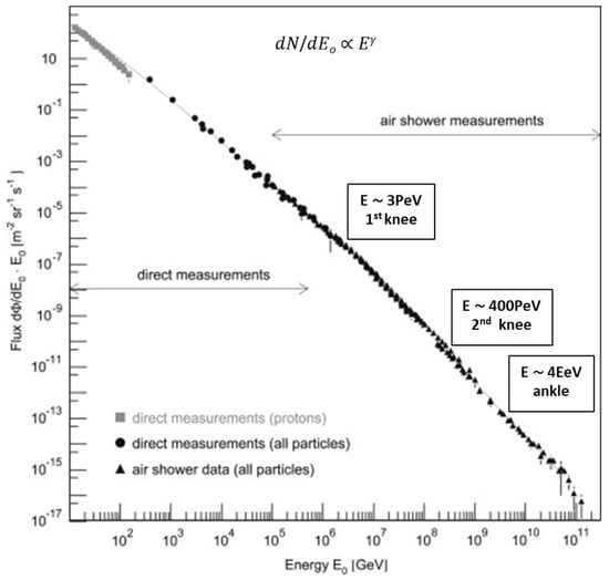
Figure 1. The differential energy spectrum of all CR particles as measured directly with detectors above the atmosphere and with air shower detectors. The spectral shape dN/dE_o ∝ E^γ breaks, known as the knee, second knee, and ankle, are indicated.

In contrast, high-energy rays have both galactic and extragalactic sources, with supernova explosions being the primary source of energy. A comprehensive account of the processes related to CR can be found in Ginzburg [1], which has remained largely unchanged since its publication.

The power-law shape of the energy spectrum across a wide range suggests the presence of non-thermal acceleration processes. This idea stems from E. Fermi’s work in 1949 [2], which proposed that CR particles are accelerated by inhomogeneities in magnetic fields, now understood as collisionless shock waves resulting from supernova explosions.

Malkov and Diamond [2] have recently formalized this concept quantitatively. Within our galaxy, the Milky Way, which contains approximately 4 × 10¹¹ stars and has an age on the order of 10¹⁰ years, such explosions occur randomly two to three times each century. Consequently, the shock waves are also random in terms of space, time, and the directions in which CR particles are propagated and accelerated, indicating a random process with uncorrelated influences in a precise sense, i.e., Markovian (e.g., [3,4]).

The CR spectrum is illustrated in Figure 1. A notable characteristic is the well-known knee: a spectral break occurring at E ∼ 3 PeV (3 × 10¹⁵ eV), which is thought to indicate the peak energy of CRs originating from the galaxy (i.e., produced within the Milky Way).

The inability of the magnetic field to capture all CR particles leads to a phenomenon where the Larmor radius approaches the galactic disk thickness. The spectral index is about 2.7 for energies below the knee and increases to around 3.1 at higher energies. Particles with energies above 3 × 10⁹ GeV are rarely observed, recorded only in isolated cases. The so-called second knee (the end of galactic dominance of ~10¹⁷−10¹⁸ eV) and the “ankle” (the beginning of extragalactic dominance of ~3 × 10¹⁸ eV) in the CR are spectral features, where the CR energy spectrum steepens and then flattens, thus marking the transition from galactic to extragalactic sources, but are not yet explained. The CR spectrum is shown in Figure 1, where the spectral breaks known as the knee (at E ∼ 3 PeV), second knee (at E ∼ 400 PeV), and ankle (at E ∼ 4 EeV) are depicted [5].

In the years 2008–2014, European and Russian scientists carried out an extensive and carefully prepared program, “PAMELA” [6]. CR spectra were measured in a range up to the knee using the satellite Resource 5. The results showed that the spectral intensity I(E) followed a power-law relationship I(E) ~ E⁻ⁿ, where the exponent, representing the differential size distribution slope, was found to be n_diff = 2.67 ± 0.02. For the integral spectrum, n was found to be n_cum = 1.67 ± 0.02, which refers to the power-law slope of the cumulative size distribution. The spread is likely smaller in this case, as cumulative spectra are generally smoother than differential spectra [4].

The interaction between CR and the Earth’s atmosphere has been a subject of long-standing scientific inquiry. Primarily, high-energy CR particles are known to penetrate the atmosphere, causing ionization. This ionization process is hypothesized to influence atmospheric chemistry and physics, with the ion-aerosol clear-sky hypothesis suggesting that it provides nuclei for cloud condensation. Understanding these intricate connections is vital for climate science and for developing predictive models for extreme weather events ([7,8,9]).

Turbulence and cascade physics act as the “filter” between CR sources (particle acceleration and particle propagation) and what we observe. Turbulent magnetic fields control how CRs propagate and shape spectral features like the knee and ankle, while cascades—in both the interstellar medium and the atmosphere—dictate how extreme CR events manifest in secondary particles. A concept diagram is given in Figure 2, showing how CR sources connect through turbulence and cascades to the observable spectrum and signals [10].

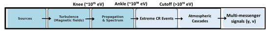
Figure 2. Schematic connection between CR sources, turbulent magnetic fields, and observable consequences. The all-particle energy spectrum shows key features—the knee (~10¹⁵ eV), ankle (~10¹⁸ eV), and cutoff (>10¹⁹ eV)—arising from acceleration limits, propagation through turbulence, and the galactic–extragalactic transition. Extreme CR events drive atmospheric cascades and produce multi-messenger signals (γ-rays, neutrinos), making the spectrum a bridge between astrophysics, fundamental physics, and atmospheric science.

It links the sources (the acceleration of CRs), the turbulent magnetic fields (shape propagation and spectral features knee-ankle-cutoff), the propagation and spectrum (what we measure as the all-particle spectrum), the extreme CR events (drive cascades), atmospheric cascades (which produce secondary radiation-muons-neutrons-isotopes), and multi-messenger signals (complementary probes of CR interactions) [11,12]. The scale-free nature, inherent to energy cascade in a turbulent medium, is the physical basis for the observed fractal and multifractal scaling in CR time series, which we investigate using DFA/MF-DFA.

Advancements in observational technology and analytical methods are broadening this research’s horizons. Initiatives like the Mini-EUSO telescope aboard the International Space Station and terrestrial facilities such as the Pierre Auger Observatory are yielding unparalleled data regarding the characteristics of cosmic rays (CRs) across a broad energy range. Additionally, experiments conducted at CERN, including the CLOUD experiment, persist in challenging and enhancing our understanding of how CRs affect aerosol particle formation in the atmosphere, indicating that certain climate models might be underestimating these impacts [7]. Machine learning is expediting the analysis of data from extensive air showers, allowing for the review of datasets that would have taken decades to process with traditional methods ([12,13]).

Recently, the temporal evolution of CRs has attracted the interest of the scientific community. It was found that it exhibits positive long-range correlations with multifractal behavior (e.g., [14,15,16]) as the global mean land and sea surface temperatures. Particularly, the attempt to forecast CR-intense events that may create severe hazards has led to the development of new analytical methods, such as “natural time” analysis, which focuses on the ordering of events rather than on conventional time, and has proven useful in nowcasting extreme events. In this context, Varotsos et al. [17] provided new evidence that CR temporal evolution follows universal scaling laws and demonstrated how “natural time” analysis can uncover links between CR variability, atmospheric oscillations, and entropy dynamics—potentially useful for forecasting extreme CR events (ECREs) and understanding their broader geophysical impacts.

Despite significant progress in CR research, key questions remain about the temporal organization of CR intensity and the mechanisms driving its abrupt variations during external or internal forcings, e.g., geomagnetic disturbances. Traditional linear and stochastic models fall short in addressing the scale-dependent correlations and non-linear behaviors found in long-term CR records. This study integrates fractal scaling analysis (DFA/MF-DFA) with Natural Time Analysis (NTA) to investigate whether self-organized criticality (SOC) and entropy dynamics can reveal the potential for their modeling in space weather research. This includes inquiries like how the observed power-law slope (≈ 3.0) of the CR energy distribution can be explained, specifically asking whether this slope is better accounted for by Kolmogorov turbulence (≈5/3 exponent) or SOC, whether these interpretations can be reconciled, and if a quantitative model exists to account for the ≈3.0 slope.

2. Materials and Methods

2.1. Observations

The Neutron Monitor Database (NMDB, Christian-Albrechts University, Kiel, in Kiel, Germany) is a global, high-resolution archive that keeps real-time cosmic ray (CR) measurements from a network of neutron monitor stations all over the world. With time resolutions as accurate as one minute, the NMDB supports detailed studies of galactic cosmic rays (GCRs) and their short- and long-term variations influenced by solar activity and heliospheric dynamics [18]. The data, gathered from a wide range of geomagnetic cut-off rigidities and altitudes, are standardized and available, making the database a key resource for examining space weather events like Forbush decreases, solar energetic particle occurrences, and daily variations in CR intensity (CRI). Besides aiding fundamental heliophysical research, NMDB data are increasingly utilized in practical fields, such as atmospheric ionization modeling, assessing radiation risks in aviation, and nowcasting space weather disturbances.

Recent studies, including those by Steigies et al. [19], have highlighted the significance and advancing capabilities of the NMDB. They show how NMDB data can be combined with analytical tools like NEST (pandas version 1.5.2) and the Python-based pandas framework (version 0.1.8) for a more flexible and efficient analysis of CR time series.

Building upon this foundation, the present study on nowcasting ECREs utilized daily CRI data from the Athens Neutron Monitor Station (A.Ne.Mo.S) over a span of 15 years, from January 2010 to December 2024. A.Ne.Mo.S is located in Athens, Greece (37.97° N, 23.78° E) at an elevation of 260 m above sea level, featuring a vertical geomagnetic cutoff rigidity of 8.53 GV. To improve the spatial and statistical reliability of the analysis, additional daily mean GCR data were obtained from another neutron monitor station: Jungfraujoch (46.55° N, 7.98° E, Switzerland) at an elevation of 3571 m above sea level. These stations were selected due to the length, continuity, and reliability of their time series, which are critical for detecting intrinsic properties of CRs and transient events. Additionally, the CR Database (CRDB) was used to enhance the dataset with historical CR fluxes gathered from various ground-based and balloon-borne experiments, enabling a more thorough analysis of CR modulation relevant to space weather real-time fractal behavior analysis.

In the following, to analyze the intrinsic properties of the CR time series, advanced analytical methods, including Detrended Fluctuation Analysis (DFA) and Multifractal Detrended Fluctuation Analysis (MF-DFA), will be employed (Figure 3). These techniques are often used to investigate self-similarity and the spectrum of singularities within the datasets [20]. Based on the fractality regime of CRs, the Natural Time Analysis (NTA) will be used to perform real-time fractal behavior analysis of the ECREs.

Figure 3. Schematic diagram of the analytical tools that are employed in the CR data analysis.

2.2. The Mono-Multifractal-Modified Detrended Fluctuation and Natural Time Analysis

To investigate the self-similarity and scaling properties of fractal signals in the CR time series, a widely used method of the DFA will be employed. It extends root-mean-square (RMS) analysis for random walks [21]. The method estimates the relationship between fluctuation size and time scale, revealing power-law correlations.

The procedure is briefly described as follows:

1.

Integrate the time series of N samples and divide it into boxes of equal length n.

2.

In each box, fit a local trend (least squares line), subtract it, and calculate the RMS fluctuation.

3.

Repeat for multiple box sizes. The function F(n) vs. n on a log–log plot gives the scaling exponent α.

For the interpretation of the result obtained, the following rules are used:

• 0.5 < α < 1 persistent correlations exist (e.g., 1/f noise at α = 1).
• 0 < α < 0.5: anti-correlations (anti-persistence) prevail.
• α > 1: correlations not of power-law type exist (α = 1.5 indicates Brownian noise).

The higher α, the smoother the signal.

A limitation of the DFA tool is that many real-world signals show different exponents at different scales (crossover behavior), requiring multifractal (MF) analysis. This is briefly described below.

The Multifractal DFA (MF-DFA) generalizes DFA to capture multifractality in finite time series, focusing on q-dependent fluctuation functions. It includes the briefly described steps [22]:

• Build the profile Y(i).
• Divide into Ns segments of length s.
• Detrend each segment using polynomial fits (DFA1, DFA2, …).
• Compute the q-order fluctuation function F_q(s).
• Analyze log–log plots of F_q(s) vs. s to obtain generalized Hurst exponents h(q) [23,24].

This is accompanied by the following key points:

• h(2) corresponds to the Hurst exponent.
• Positive q indicates scaling of large fluctuations, while negative q: small fluctuations.
• For monofractals, h(q) is independent of q; for multifractals, it varies.

An extension of the MF-DFA is the modified MF-DFA, which improves accuracy for strongly anti-correlated signals by integrating the series before analysis. Its applications include climate, sea level, and drought variability studies (e.g., [24,25]).

Finally, the concept of natural time will be employed, which allows the exploration and analysis of complex observational data in real time. It was introduced by Varotsos et al. [25] and employed to investigate the dynamics of complex systems. It is particularly useful for systems that exhibit critical behavior and extreme events. Time series analysis is usually about events happening on a straight line. Natural time is different. It looks at how things happen based on the order and how important they are. Each event contributes proportionally to its “energy” or intensity, allowing hidden correlations and precursors to emerge more clearly. In this framework, each event in a sequence is assigned a normalized index. To implement the nowcasting of the CR time series, the NTA is employed. Instead of using conventional (clock) time, it represents events by their order and energy contribution.

3. Results and Discussion

3.1. The Long-Range Correlations in CR Dynamics

The CR time series recorded at the Athens Neutron Monitor Station (Athens NM 64), which belongs to the A.Ne.Mo.S, was analyzed using the DFA2 method. The profile of the derived root-mean-squared fluctuation function $F_d\left(\tau \right)$ versus time scale $\tau$(in days), is shown in Figure 4a. From this analysis, we obtained a scaling exponent α = 1.03 ± 0.01, which indicates the presence of persistent long-range temporal correlations characteristic of 1/f—type (pink noise). Establishing genuine power-law long-range correlations requires more than a single exponent; specifically, it necessitates rejecting the alternative hypothesis of exponential decay in the autocorrelation function and verifying the constancy of local slopes within a sufficiently broad scale range toward low frequencies, as discussed in Maraun et al. [26].

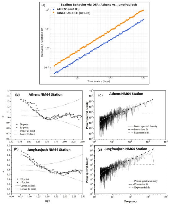
Figure 4. (a) The F_d (τ) of DFA2 in a log–log plot for the Athens NM64 Station with the fit equation ψ = 1.03χ − 1.62 (R² = 0.992) and for the Jungfraujoch NM64 Station (bottom) with ψ = 1.07χ − 1.22 (R² = 0.994). (b) Local slopes α of logF_d (τ) vs. logτ for both stations, indicating 2σ intervals with dashed gray lines. (c) The power spectral density for the Athens NM64 Station includes power-law and exponential fits, with ψ values of ψ = 7.81 × 10⁻⁷χ^−1.36 (R² = 0.50) and ψ = 4.79 × 10⁻⁵ e^−7.1χ (R² = 0.35). For Jungfraujoch NM64 Station, the fits are ψ = 4.23 × 10⁻⁵χ^−1.75 (R² = 0.49) and ψ = 1.09.79 × 10⁻² e^−9.9.1χ (R² = 0.56).

To investigate this further, we assessed the local scaling behavior of the fluctuation function by calculating the local slopes of $\log F_d\left(\tau \right)$ versus $\log \tau$. This was achieved using moving windows of 15 and 20 points, which were shifted stepwise across all scales $\tau$ to test for the slope constancy.

To benchmark this, we performed Monte Carlo simulations using DFA2 on 500 synthetic time series. Each time series was generated as fractional Gaussian noise with a consistent scaling exponent $\alpha =1.03$ [26]. For each simulation, we calculated the local slopes $\alpha \left(\tau \right)$ using a consistent windowing approach.

The Kolmogorov–Smirnov [27,28] and Anderson–Darling [29] best-fit tests confirmed that, at each fixed time scale $\tau$, the distribution of local slopes $\alpha \left(\tau \right)$ followed a Gaussian distribution at the 95% confidence level. Based on this finding, confidence bands were defined as $\alpha \left(\tau \right)\pm 2{\sigma }_{\alpha \left(\tau \right)}$, where ${\sigma }_{\alpha \left(\tau \right)}$ is the standard deviation derived from the ensemble of simulated local slopes.

To further assess the stationarity of the scaling behavior, we determined a confidence range $R$ for the local slopes of the CR time series by calculating the empirical mean ± 2 standard deviations. This can be expressed mathematically as follows:

$$R=\left(\alpha \left(\tau \right)-2{\sigma }_{\alpha \left(\tau \right)},\alpha \left(\tau \right)+2{\sigma }_{\alpha \left(\tau \right)}\right)$$

(1)

As illustrated in Figure 4b (top), all local slopes for scales beyond $\log \tau =1.6$ fall within this confidence range $R$. This finding confirms sufficient scale-invariant behavior across a broad temporal range.

Additionally, to complement the DFA2 analysis, we computed the power spectral density (PSD) of the CR time series, which is presented in Figure 4c (top). The PSD profile clearly exhibits a power-law decay, with a significantly higher coefficient of determination (R²) for the power-law fit compared to the exponential fit. This further satisfies the criteria set forth by Maraun et al. [26] for identifying long-range power-law correlations.

To confirm that the observed persistence (i.e., $\alpha =1.03$) arises from the temporal ordering of the CR data, rather than from its marginal distribution, we conducted a random shuffling test. The CR time series was randomly shuffled 1000 times, which disrupted temporal correlations while maintaining the distribution of values. We then applied the DFA2 to each shuffled series to extract the distribution of shuffled exponents ${\alpha }^{\mathrm{’}}$. The resulting distribution of ${\alpha }^{\mathrm{’}}$ values was tested using the Kolmogorov–Smirnov and Anderson–Darling tests, confirming normality at the 95% confidence level. The standard deviation of this distribution was found to be ${\sigma }_{{\alpha }^{\mathrm{’}}}=0.06$, and we computed the 95% confidence interval for the mean exponent under white-noise conditions as follows:

$${\alpha }^{\mathrm{’}}\pm 1.96{\displaystyle \frac{{\sigma }_{{\alpha }^{\mathrm{’}}}}{\sqrt{1000}}}$$

(2)

Notably, the originally estimated exponent $\alpha =1.03$ and lies well outside this confidence interval. According to the t-test, this statistically excludes the possibility that the observed scaling behavior arises from a white-noise process. Thus, we conclude with high confidence that the CR time series at Athens exhibits genuine long-range persistence of power-law type.

For comparison, we applied the same analysis to the CR time series at Jungfraujoch Station. The corresponding root-mean-square fluctuation function F_d (τ) obtained from the DFA2 technique against the time scale τ (in days) is shown in Figure 4a. The scaling exponent stemming from the DFA2 tool for this time series is nearly equal to that of the CR time series at the Athens station, further suggesting persistent memory of 1/f—type behavior.

However, to establish the power-law long-range correlations for the CR time series from Jungfraujoch, we investigated whether the two criteria proposed by Maraun et al. [26] are satisfied.

We specifically evaluated the local slopes of logF_d (τ) vs. logτ, which fall within the range R across all calculated scales τ, further indicating a sense of constancy (Figure 4b bottom).

In contrast, a power-law fit on the profile of the power spectral density for the CR time series at Jungfraujoch provided a better coefficient of determination than the exponential fit (Figure 4c, bottom). Consequently, both criteria proposed by Maraun et al. [26] indicate that the CR time series at Jungfraujoch station exhibits long-range correlations of a power-law type.

The above-mentioned analyses of CR data revealed distinct scaling features. The time series demonstrated positive long-range correlations of a 1/f type behavior. This finding indicates a persistent, complex, and non-linear dynamic to CRI. Additionally, this fractality appears to be more significantly influenced by solar activity and geomagnetic events than by the station’s geographic location.

In the following, we analyze the spectrum of singularities for the Athens CR time series, using the MF-DFA. In this context, the MF-DFA2 technique specifically utilizes the second moment (q = 2) to compute the q-th order fluctuation function, Fq(τ), for various moments q. The scaling behavior of Fq(τ) (i.e., the slope) for all selected positive and negative moments q remains nearly consistent for logτ > 2 (where τ > 100). However, this consistency does not hold for smaller time scales (τ < 100), where the slope of Fq(τ) increases for less positive (more negative) moments q. This behavior shows significant multifractality at short time scales (τ ≤ 100). Larger windows average out local fluctuations, both small and large, resulting in diminished differences in magnitude [9].

The above suggested multifractality is illustrated where the generalized Hurst exponent h(q) for the Athens CR time series varies versus q-values (i.e., h(q) is not independent of q), while the h(q) values, which are higher than 0.5, indicate long-term persistence for the examined time series. Moreover, the slope of h(q) for positive moments seems to be similar to that of negative moments. Figure 5 presents the singularity spectrum f(n) as a function of the singularity strength n for the examined Athens CR time series [22].

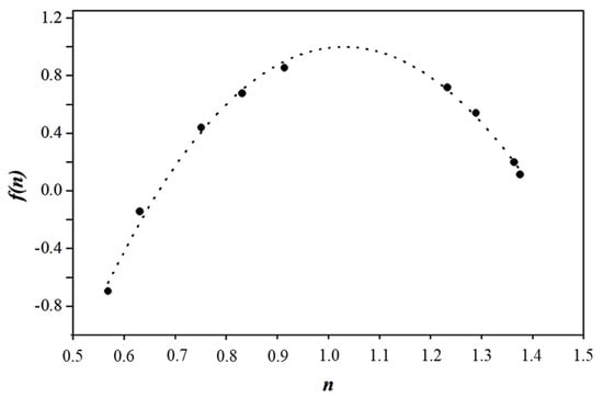
Figure 5. The singularity spectrum f(n) versus singularity strength n for the examined time series. The empirical curve (dots) is fitted by the polynomial of third order (y = 0.63x³ − 9.1x² + 18.1x − 8.97 with R² = 0.987) (dashed line).

To quantify the multifractality, the width of the singularity spectrum Δn = n_max = n_min is assessed. A non-zero width quantitatively confirms the multifractal nature2. The maximum value of f(n) corresponds to q = 0, while f(n) values on the left (right) of the maximum value correspond to positive (negative) moments q. It is apparent that f(n) fluctuates similarly on both sides of its maximum value. This fact once more reveals common features of multifractality for positive and negative q-values.

3.2. Warning Signatures of ECREs: The Forbush Effect of May 2024

The successive compressions of the fractal memory into long-, medium-, and real-time inference are prediction, forecasting, and nowcasting. We are generally more familiar with “forecast” than “nowcast.” Here is a brief overview of the time scales and data sources for both. As illustrated in Figure 6, nowcasting (shown in red) refers to a time scale of up to 6 h, and it uses real-time satellite data to track solar particles and X-ray bursts. Short-term forecasting (shown in blue) refers to a time scale, from 6 h to 3 days, and it is based on monitoring solar flares, coronal mass ejections, and heliospheric models. Finally, the long-term forecasting (shown in green) refers to a time scale from weeks to months, and it relies on sunspot cycles, magnetic field changes, and statistical solar activity models. Both approaches have limitations. As far as the forecast limitation is concerned, predicting particle acceleration near the Sun is challenging due to the complexity of the modeling. The nowcast limitation refers to the fact that it offers minimal warning, as high-energy particles can reach Earth within minutes of a solar flare.

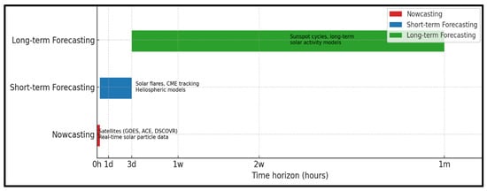
Figure 6. Real-time fractal behavior analysis—nowcasting uses real-time satellite data to track solar particles and X-ray bursts. Short-term forecasting monitors solar flares and coronal mass ejections. Long-term forecastingrelies on sunspot cycles and magnetic field changes.

On 10–11 May 2024, a significant geomagnetic storm occurred, accompanied by a substantial decrease in GCR intensity, which sparked scientific curiosity due to its rarity. This event was particularly noteworthy because a comparable occurrence was last observed nearly two decades prior (see [30] for further details).

The Forbush Effect (FE) is characterized by a sudden decrease in GCR intensity, followed by a gradual increase. This increase is sometimes accompanied by local increases in particle flux, caused either by solar-accelerated protons or by the modulation of GCRs by the interplanetary medium and magnetosphere. Such superimposed effects were observed during intense solar activity in early May 2024, when active region flares occurred, some of which were accompanied by coronal mass ejections [31]. According to the data analysis shown in Figure 7, an interplanetary shock wave reached Earth on 10 May, raising solar wind velocity to ~750 km/s and magnetic field strength to ~70 nT. NASA’s Advanced Composition Explorer (ACE) collects and analyzes particles from solar, interplanetary, interstellar, and galactic origins [32].

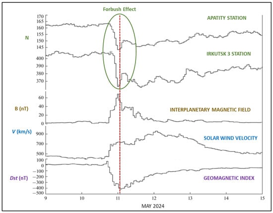
Figure 7. Variations in CR during the extreme geomagnetic disturbances on 9–15 May 2024. CR variations on 9–15 May 2024, detected by neutron monitors at Apatity station and Irkutsk 3 station in relative units. Hourly data on interplanetary magnetic field B, solar wind velocity V, and geomagnetic index Dst are given in the lower part of the figure.

On 12 May 2024, a solar wind speed increase of 989 km/s triggered a major geomagnetic storm, the strongest since 2003. The Dst index dropped to −412 nT, and Kp reached ~9 by May 11. This caused a pronounced Forbush Effect, detected by global neutron monitors, with the FE onset on May 10 and GCR flux recovery on May 11.

According to the current literature, predictors appearing hours to days before the May 2024 geomagnetic storm show that combining multiple solar-terrestrial indicators is key for reliable fractal temporal dynamics of powerful space weather disturbances (e.g., [32]).

3.2.1. Real-Time Fractal Behavior Analysis: The Importance of Order, Not Time, of ECRE Occurrence

Building on the confirmed fractal dynamics of CR intensity, we utilize the NTA tool, which is specifically designed to detect critical phenomena by focusing on the order and “energy” (intensity) of events, providing a complementary approach to scaling analysis. A sophisticated idea is to convert the CR time series shown on the top of the upper part of Figure 8 to a new series shown just below it as follows: with (1), we define an index χ_k = k/i, where k is the order of occurrence of each event and i is the total number of events. The second step is to analyze the evolution of the pair (χ_k, Q_k), where Q_k is the energy of the kth event, and then define probabilities with (2). The average quantities are derived from (3), and with (4), the entropy S in natural time is calculated at different intervals of natural time. Next, the entropy S- under time reversal is calculated using (5). Finally, we explore the difference ΔSi, denoting the dynamics, when transitioning from the present to the future and vice versa [33,34].

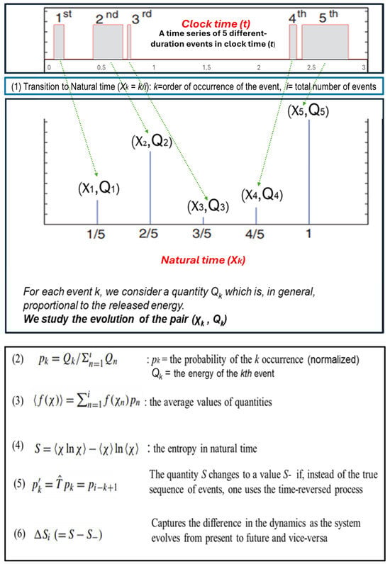
Figure 8. The top graph shows five CR events over time, while the bottom graph represents the time domain, χ_k, as the ratio of occurrence k to total events N. It analyzes pairs (χ_k, Q_k). Average values are calculated using (3), and entropy S is derived from (4) for various time intervals. Time-reversed entropy S- is calculated with (5), allowing the exploration of the dynamics difference ΔSi from present to future and vice versa.

Briefly, the core idea of NTA may be described as follows:

• Each event is assigned a normalized “natural time” χ_k = k/i, where k is the event index and i is the total number of events.
• The energy (or other quantity of interest) of each event is incorporated as a weight.

The key quantities of NTA are the following:

• The variance of natural time, κ₁, is linked to correlations and criticality.
• The entropy S in natural time evaluates complexity and information content.

NTA has been applied for the following:

• Detecting precursors of critical transitions (e.g., earthquakes, O₃ hole, mean sea level) [35].
• Characterizing long-range correlations and self-organized criticality [36].
• Complementary to DFA/MF-DFA for scaling and multifractal behavior.

The primary advantage of NTA is the following: by focusing on event order and energy rather than conventional time, NTA highlights hidden correlations and critical features that may be invisible in conventional time series analysis.

The entropy difference in natural time, expressed as ΔSi = Si − (S_)I, was evaluated over temporal windows ranging from 3 to 15 h during May 2024. For this, a window of length (i) was sliding each time by one hour through the whole time series, each time calculating the entropy S. We repeat this calculation upon considering the time reversal S_. A clear scale-invariant behavior of ΔSi was observed before 10 May for shorter time scales (3–7 h), where ΔSi approaches zero. Notably, the convergence of both entropy measures on 10 May suggests the presence of a precursor signal, occurring around 3–7 h before the Forbush decrease event depicted in Figure 7.

It is worth noting that, as shown in Figure 8, the equations reveal a quantity that enables the identification of a dynamical system’s approach to the critical state, which is difficult to determine using other methods. In particular, it can be shown that the quantity κ₁ = <χ²> − <χ>², that is, the variance in natural time, equals 0.070 at the critical state for various dynamical systems. In addition, when the distribution is uniform, both entropies Si = (S_)i become equal to 0.0966. When the system approaches the critical dynamics, then both entropies are lower than 0.0966. It is important to mention that k₁ is non-zero before the occurrence of a strong CR event (phase change), while k₁ becomes zero upon the occurrence of a strong CR event.

Consequently, NTA applied to CR data during May 2024 detected entropy convergence 3–7 h before the Forbush decrease. The variance κ₁ approached the critical threshold of 0.070, while entropy values decreased below 0.0966, marking the system’s transition toward criticality. These signatures indicate that NTA can identify phase transitions in real-time data.

3.2.2. The Long-Term Signal for the Forbush Event Phase Transition

Varotsos et al. [17] investigated the relationship between entropy S and the power-law exponent γ characterizing the temporal evolution of CR flux, using NTA. We employ the same analysis using more observations to derive a fractal temporal dynamics tool for ECRE. The entropy values were computed within a 2-year (730-day) sliding window, moving forward one day at a time. The selection of this window length aligns with the Quasi-Biennial Oscillation (QBO), a 2–3-year atmospheric cycle that modulates stratospheric dynamics and potentially influences CR flux reaching the ground.

As shown in Figure 9, the power-law exponent γ of the power spectral density of the entropy sequence was determined for each window. Results showed that γ ranges from −1.74 to −1.57, with an entropy value (S₇₃₀ = 0.0966) at γ = −1.67 (≈−5/3)—a hallmark of a stationary system emitting uncorrelated energy bursts. It should be remembered that the entropy of the uniform distribution S_u can be calculated as follows: S_u = (ln2)/2 − 1/4 ≈ 0.0966. Therefore, S₇₃₀ = S_u.

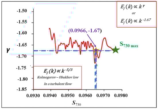
Figure 9. Power-law exponent $\gamma$ of the energy values $E_j\left(j=\mathrm{1,2},\dots ,730\right)$ as a function of frequency versus $S_{730}$. The analysis is based on a 730-point sliding window applied to the entire CR time series, which is expressed as a 30-day running mean (red line). Notably, one of the data points with $S_{730}=S_u=0.0966$ corresponds to $\gamma =-5/3\approx -1.67$(highlighted by the blue coordinates and purple star). So, the entropy rises to the point marked by the purple star, representing a uniform distribution (S_u). Then, it reaches its peak at the Kolmogorov–Obukhov exponent of –5/3, marking the phase transition, where the Forbush Event occurred (green star).

To address the potential confusion regarding the two power-law exponents presented in Figure 9, we clarify the fundamental difference in the physical quantities and domains they represent: The power spectrum E(k), characterized by the Kolmogorov exponent of −5/3 (or ≈−1.67), is a dynamic measure in Fourier space and describes the distribution of turbulent energy across spatial scales (wavenumber, k)—a key feature of fluid dynamics and the energy cascade. In contrast, the differential size distribution n_diff (E), with the observed exponent of ≈−3.0, is a statistical measure in event space that quantifies the occurrence frequency of events as a function of their magnitude (energy, E). As discussed by Bak et al. [37,38], this latter exponent is a characteristic signature of complex systems exhibiting SOC, where it captures the statistics of discrete energy-release events (small vs. large avalanches). While both exponents represent power-law scaling, they apply to distinct physical domains and describe separate phenomena (energy cascade in turbulence vs. event magnitude statistics in SOC systems) [4].

Quantitatively, the observed slope of ≈3.0 in the CR energy distribution can be understood as the combined outcome of diffusive shock acceleration (DSA) and energy-dependent propagation through a turbulent interstellar medium. In DSA, strong shocks produce a source spectrum ∝ E^−s with s ≈ 2.0–2.4 [39,40]. During propagation, scattering by magnetic turbulence characterized by a Kolmogorov spectrum (∝k^−5/3) yields a diffusion coefficient D(E)∝E^δ with δ ≈ 1/3 [41]. The resulting steady-state differential spectrum follows N(E)∝E^−(s+δ), producing total slopes n ≈ 2.7–3.0, in agreement with observations.

Alternatively, within the SOC framework, the same slope naturally emerges from scale-free avalanche statistics, where the distribution of event energies reflects the fractal geometry and diffusion-like transport of energy in a near-critical plasma [4,42]. In this interpretation, turbulence supplies the physical driver that maintains the system near criticality, while SOC describes the statistical distribution of intermittent acceleration or reconnection events. Thus, the turbulence-based transport and SOC-based event statistics are not mutually exclusive, but represent complementary aspects of a single, turbulence-driven, near-critical astrophysical system.

The observed γ ≈ −5/3 behavior aligns with findings in other complex systems such as solar flares, earthquakes, and icequakes, indicating self-organized criticality in CR temporal dynamics. Environmental factors—including barometric pressure, temperature, and humidity—modulate CR secondary particle production and neutron intensity. These findings underscore the potential of NTA for predicting ECREs and highlight the broader interconnection between CR variability, atmospheric processes, and climate dynamics [43].

Therefore, Figure 9 shows how entropy varies with the energy exponent γ. It is obvious that, at this window, the entropy varies around −1.67, which is not a random number. It equals −5/3, the exponent proposed by Kolmogorov and Obukhov in 1941. As shown in the figure, the entropy increases, reaching the point with the purple star, which signifies the state of uniform distribution. Then the entropy is maximized, at the Kolmogorov and Obukhov exponent −5/3, denoting a phase transition, where the Forbush Event took place (shown with the green star). This means that this tool can provide the fractal temporal dynamics of an ECRE around two years ahead.

In summary, the analysis reveals a significant correlation between entropy and the energy exponent γ, particularly highlighting the critical role of the Kolmogorov and Obukhov exponent in inferring phase transitions during the Forbush Event. This finding underscores the potential of the tool to forecast an ECRE up to two years in advance, marking a notable advancement in our understanding of entropy dynamics.

3.2.3. The Order of ECREs for the Future Occurrence Rate

Varotsos et al. [44] proposed the Modified Natural Time Analysis (M-NTA) to forecast the occurrence rate of future extreme events. The M-NTA involves the following steps: Initially, the cumulative number (C_N) of CR values equal to or exceeding a specific x-value is computed. Subsequently, the logarithm of C_N is plotted against the x magnitude, and regression analysis is conducted on the log (C_N) versus x plot to unveil the distribution of CR anomalies. Following this, the NTA is employed to examine exceptional events within the time series of CR anomalies.

By disregarding clock time and focusing on “natural time”, an index is generated representing the order of occurrence of an event divided by the total number of events in the time series. Consequently, high CR values (with x ≥ x₂) are identified in the studied time series, and the cumulative numbers C_N1 and C_N2 of CR values with magnitude x ≥ x₁ and x ≥ x₂, respectively (where x₁ < x₂), occurring after this high CR value until the end of the time series, are calculated.

Plotting the pairs (C_N1, C_N2), a perfect linear fit f(C_N1) = A·C_N2 yields. The above-mentioned technique allows us to precisely test the accuracy of the GR fit by examining whether two values with a constant difference x₂ − x₁ have a constant ratio:

C_N2/C_N1 = 10^a_○^·(x₂^−x₁⁾ = constant.

Finally, using the above results, the occurrence rate C_N′/t = 10^a_○^·(x_○^−x₁⁾·b, and consequently the average time interval between two successive CR values with x ≤ x₀ can be forecasted. For more information, see the analysis presented in Varotsos et al. [44].

By applying this technique, the two successive extreme CR events (Forbush decreases and geomagnetic storms) that took place on 24 March 2024 and 11 May 2024 can be forecasted. In more concrete terms, the aforementioned M-NTA model is capable of nowcasting the subsequent CR Forbush Event following the one that occurred on 24 March 2024. It seems to effectively estimate the anticipated time (or interevent time) between consecutive events.

Based on the calculations provided, it was determined that the average recurrence time for the next Forbush Event falls within the range of (1080, 1200) hours (approximately 45–50 days). In fact, the subsequent event occurred on 11 May 2024, which is 48 days later.

4. Conclusions

The present comprehensive analysis confirms that the CRI time series exhibits multifractal dynamics with persistent long-range correlations with a scaling characteristic of 1/f-type (pink) noise [38]. This robust finding indicates a persistent, complex, and non-linear dynamic to CRI, which appears to be more significantly influenced by solar activity and geomagnetic events than by the station’s geographic location.

A key contribution of this study is the application of the NTA tool, demonstrating its operational utility for the nowcasting of ECREs. Through the case study of the 9–15 May 2024, geomagnetic storm and Forbush decrease, the NTA entropy difference converged to zero at short time scales (3–7 h) on 10 May, providing an early-warning precursor signal approximately 3–7 h before the event onset revealed by the entropy maximization.

The M-NTA estimated the recurrence interval between two major Forbush events (24 March and 11 May 2024) as approximately 47.5 days—remarkably close to the observed 48-day interval—highlighting the model’s reliability in estimating interevent times for solar CR fluctuations.

Furthermore, the NTA-derived link between entropy and the power-law exponent of the CR flux time series provides a powerful long-term forecasting tool for critical transitions. Specifically, the occurrence of the Forbush Event coincided precisely with the maximization of entropy, a finding characteristic of a phase transition and the critical state (SOC) in complex systems. Notably, this evidence of a critical transition was temporally coincident with the CR dynamics exhibiting a power-law exponent (spectral index) of −5/3 ≈ −1.67, which is characteristic of fully developed Kolmogorov turbulence. This NTA-based analysis not only establishes a clear link between entropy dynamics and critical transitions but also indicates the tool’s potential to forecast an Extreme Cosmic Ray Event (ECRE) up to two years in advance, significantly enhancing our understanding and prediction capability. Collectively, this integration of fractal scaling and advanced analytical techniques furnishes a deeper understanding of the complex, underlying physical processes governing CR variations.

In summary, this study demonstrates that CR intensity fluctuations exhibit multifractal dynamics and persistent correlations of the 1/f type. By integrating scaling analysis with natural time entropy, early-warning and long-term capabilities for ECRE detection have been established. The convergence of entropy near γ ≈ −5/3 marks phase transitions in CR flux, linking microscopic acceleration processes with macroscopic variability. These results suggest that NTA-based models can enhance insights into space weather and heliophysical research. In prior research, several geophysical parameters had already been found to exhibit clear multifractal behavior and varying degrees of persistence. For instance, both the Indian Summer Monsoon Rainfall and total ozone data display pronounced multifractality, with entropy analysis revealing that the entropy-maximizing approach provides a more accurate representation of their variability than traditional statistical methods (e.g., normal distribution fitting). Given these precedents, it would therefore be of considerable interest for future studies to apply the present findings to the analysis of Indian Summer Monsoon Rainfall and total ozone variability [45,46,47].

References

- Ginzburg, V.L. (Ed.) Astrophysics of Cosmic Rays; English ed.; North Holland Publ. Co.: Amsterdam, The Netherlands, 1990. [Google Scholar]
- Malkov, M.A.; Diamond, P. Modern theory of Fermi acceleration: A new challenge to plasma physics. Phys. Plasmas 2001, 8, 2401–2406. [Google Scholar] [CrossRef]
- Varotsos, C.A.; Golitsyn, G.S.; Efstathiou, M.; Sarlis, N. A new method of nowcasting extreme cosmic ray events. Remote Sens. Lett. 2023, 14, 576–584. [Google Scholar] [CrossRef]
- Golitsyn, G.; Varotsos, C. The Stochastic Nature of Environmental Phenomena and Processes; Springer: Berlin/Heidelberg, Germany, 2025. [Google Scholar] [CrossRef]
- Blümer, J.; Engel, R.; Hörandel, J.R. Cosmic rays from the knee to the highest energies. Prog. Part. Nucl. Phys. 2009, 63, 293–338. [Google Scholar] [CrossRef]
- Karelin, A.V.; Adriani, O.; Barbarino, G.C.; Bazilevskaya, G.A.; Bellotti, R.; Boezio, M.; Bogomolov, E.A.; Boneci, L.; Bongi, M.; Bonvicini, V.; et al. New measurements of the energy spectra of protons and helium nuclei of high-energy cosmic rays using a calorimeter in the PAMELA experiment. J. Exp. Theor. Phys. 2014, 119, 448–452. [Google Scholar] [CrossRef]
- Varotsos, C.; Tzanis, C.; Cracknell, A. The Enhanced Deterioration of the Cultural Heritage Monuments Due to Air Pollution. Environ. Sci. Pollut. Res. 2009, 16, 590–592. [Google Scholar] [CrossRef] [PubMed]
- Varotsos, C.A.; Golitsyn, G.S.; Xue, Y.; Efstathiou, M.; Sarlis, N.; Voronova, T. On the relation between rain, clouds, and cosmic rays. Remote Sens. Lett. 2023, 14, 301–312. [Google Scholar] [CrossRef]
- Christodoulakis, J.; Varotsos, C.A.; Mavromichalaki, H.; Efstathiou, M.N.; Gerontidou, M. On the link between atmospheric cloud parameters and cosmic rays. J. Atmos. Sol.-Terr. Phys. 2019, 189, 98–106. [Google Scholar] [CrossRef]
- Varotsos, C.A.; Golitsyn, G.S.; Efstathiou, M.; Sarlis, N. The remotely sensed geometric data of rain and clouds as a basis for studying extreme events. Remote Sens. Lett. 2023, 14, 558–564. [Google Scholar] [CrossRef]
- Loftfield, J.; Nowaczyk, N.; Lembke-Jene, L.; Frederichs, T.; Lachner, J.; Lamy, F.; Rugel, G.; Stübner, K.; Adolphi, F. Constraints on the use of cosmogenic beryllium isotopes for synchronizing marine sediments and ice cores. Earth Planet. Sci. Lett. 2025, 671, 119665. [Google Scholar] [CrossRef]
- CERN. CLOUD Challenges Current Understanding of Aerosol Particle Formation in Polar and Marine Regions. CERN, 15 December 2023. [Google Scholar]
- CERN. Cosmic Count Exceeds Expectation. CERN, 13 August 2024. [Google Scholar]
- Sierra-Porta, D. On the fractal properties of cosmic rays and Sun dynamics cross-correlations. Astrophys. Space Sci. 2022, 367, 116. [Google Scholar] [CrossRef]
- Efstathiou, M.N.; Tzanis, C.; Cracknell, A.P.; Varotsos, C.A. New features of land and sea surface temperature anomalies. Int. J. Remote Sens. 2011, 32, 3231–3238. [Google Scholar] [CrossRef]
- Giri, A.; Adhikari, B.; Dahal, S.; Paula, K.S.S.; Bolzan, M.J.A. Multifractal Analysis of Cosmic Rays over Mid- and High-Latitude Stations During Severe Geomagnetic Storms. Sol. Phys. 2024, 299, 148. [Google Scholar] [CrossRef]
- Varotsos, C.A.; Golitsyn, G.S.; Mazei, Y.; Sarlis, N.V.; Xue, Y.; Mavromichalaki, H.; Efstathiou, M.N. On the observed time evolution of cosmic rays in a new time domain. Acta Astronaut. 2024, 225, 436–443. [Google Scholar] [CrossRef]
- Mavromichalaki, H.; Papaioannou, A.; Plainaki, C.; Sarlanis, C.; Souvatzoglou, G.; Gerontidou, M.; Tziotziou, K. Applications and usage of the real-time Neutron Monitor Database (NMDB). Adv. Space Res. 2011, 47, 2210–2222. [Google Scholar] [CrossRef]
- Steigies, C.T.; Fuller, N.; The NMDB Team. Accessing NMDB data using NEST and pandas. In Cosmic Ray Studies with Neutron Detectors; Kiel University: Kiel, Germany, 2023; Available online: https://macau.uni-kiel.de/receive/macau_mods_00003844 (accessed on 13 November 2025).
- Maejim, E. An introduction to the theory of self-similar stochastic processes. Int. J. Mod. Phys. B 2000, 14, 1399–1420. [Google Scholar] [CrossRef]
- Peng, C.K.; Buldyrev, S.V.; Havlin, S.; Simons, M.; Stanley, H.E.; Goldberger, A.L. Mosaic organization of DNA nucleotides. Phys. Rev. E 1994, 49, 1685. [Google Scholar] [CrossRef]
- Kantelhardt, J.W.; Zschiegner, S.A.; Koscielny-Bunde, E.; Havlin, S.; Bunde, A.; Stanley, H.E. Multifractal detrended fluctuation analysis of nonstationary time series. Phys. A Stat. Mech. Appl. 2002, 316, 87–114. [Google Scholar] [CrossRef]
- Hurst, H.E. Long-term storage capacity of reservoirs. Trans. Am. Soc. Civ. Eng. 1951, 116, 770–799. [Google Scholar] [CrossRef]
- Pachore, A.B.; Remesan, R.; Kumar, R. Multifractal characterization of meteorological to agricultural drought propagation over India. Sci. Rep. 2024, 14, 18889. [Google Scholar] [CrossRef]
- Varotsos, P.A.; Sarlis, N.V.; Skordas, E.S. Long-range correlations in the electric signals that precede rupture. Phys. Rev. E 2002, 66, 011902. [Google Scholar] [CrossRef]
- Maraun, D.; Rust, H.W.; Timmer, J. Tempting long-memory—On the interpretation of DFA results. Nonlinear Process Geophys. 2004, 11, 495–503. [Google Scholar] [CrossRef]
- Timmer, J.; Koenig, M. On generating power law noise. Astron. Astrophys. 1995, 300, 707. [Google Scholar]
- Stephens, M.A. EDF statistics for goodness of fit and some comparisons. J. Am. Stat. Assoc. 1974, 69, 730–737. [Google Scholar] [CrossRef]
- Anderson, T.W.; Darling, D.A. A test of goodness of fit. J. Am. Stat. Assoc. 1954, 49, 765–769. [Google Scholar] [CrossRef]
- Makhmutov, V.S.; Bazilevskaya, G.A.; Philippov, M.V.; Stozhkov, Y.I.; Erkhov, V.I.; Morzabaev, A.K.; Tulekov, Y.A.; Raulin, J.P.; Tacza, J. Variations in Cosmic Rays during the Extreme Geomagnetic Disturbances of May 9–15, 2024. Bull. Russ. Acad. Sci. Phys. 2025, 89, 830–834. [Google Scholar] [CrossRef]
- Mavromichalaki, H.; Papailiou, M.C.; Livada, M.; Gerontidou, M.; Paschalis, P.; Stassinakis, A.; Abunina, M.; Shlyk, N.; Abunin, A.; Belov, A.; et al. Unusual forbush decreases and geomagnetic storms on 24 March, 2024 and 11 May, 2024. Atmosphere 2024, 15, 1033. [Google Scholar] [CrossRef]
- NASA. Annual Highlights of Results from the International Space Station. 2024. Available online: https://www.nasa.gov/wp-content/uploads/2025/02/ahr-2024-final.pdf (accessed on 13 November 2025).
- Borog, V.V.; Astapov, I.I.; Barbashina, N.S.; Mishutina, Y.N.; Shutenko, V.V. Analysis of Geoeffective Coronal Mass Ejections in the Flux of the Solar Wind and Cosmic Rays at Ground Level on May 10–12, 2024. Bull. Russ. Acad. Sci. Phys. 2025, 89, 821–825. [Google Scholar] [CrossRef]
- Varotsos, P.A.; Sarlis, N.V.; Skordas, E.S. Order Parameter Fluctuations in Natural Time and B-Value Variation Before Large Earthquakes. Nat. Hazards Earth Syst. Sci. 2012, 12, 3473–3481. [Google Scholar] [CrossRef]
- Nikolopoulos, D.; Cantzos, D.; Alam, A.; Dimopoulos, S.; Petraki, E. Electromagnetic and radon earthquake precursors. Geosciences 2024, 14, 271. [Google Scholar] [CrossRef]
- Varotsos, P.A.; Sarlis, N.V.; Skordas, E.S.; Tanaka, H.A. Plausible Explanation of the B-Value in the Gutenberg-Richter Law from First Principles. Proc. Jpn. Acad. Ser. B 2004, 80, 429–434. [Google Scholar] [CrossRef]
- Bak, P.; Tang, C.; Wiesenfeld, K. Self-organized criticality: An explanation of the 1/f noise. Phys. Rev. Lett. 1987, 59, 381. [Google Scholar] [CrossRef]
- Bak, P.; Tang, C.; Wiesenfeld, K. Self-organized criticality. Phys. Rev. A 1988, 38, 364. [Google Scholar] [CrossRef] [PubMed]
- Blandford, R.; Eichler, D. Particle acceleration at astrophysical shocks: A theory of cosmic ray origin. Phys. Rep. 1987, 154, 1–75. [Google Scholar] [CrossRef]
- Caprioli, D. Cosmic-ray acceleration in supernova remnants: Non-linear theory revised. J. Cosmol. Astropart. Phys. 2012, 2012, 038. [Google Scholar] [CrossRef]
- Berezinskii, V.S.; Bulanov, S.V.; Dogiel, V.A.; Ginzburg, V.L.; Ptuskin, V.S. Astrophysics of Cosmic Rays; Izdatel’stvo Nauka: Moscow, Russia, 1984. [Google Scholar]
- Aschwanden, M.J. A macroscopic description of a generalized self-organized criticality system: Astrophysical applications. Astrophys. J. 2014, 782, 54. [Google Scholar] [CrossRef]
- Tsonis, A.A.; Deyle, E.R.; May, R.M.; Sugihara, G.; Swanson, K.; Verbeten, J.D.; Wang, G. Dynamical evidence for causality between galactic cosmic rays and interannual variation in global temperature. Proc. Natl. Acad. Sci. USA 2015, 112, 3253–3256. [Google Scholar] [CrossRef]
- Varotsos, C.; Sarlis, N.V.; Mazei, Y.; Saldaev, D.; Efstathiou, M. A composite tool for forecasting El Niño: The case of the 2023–2024 event. Forecasting 2024, 6, 187–203. [Google Scholar] [CrossRef]
- Chakraborty, S.; Chattopadhyay, S. Exploring the Indian summer monsoon rainfall through multifractal detrended fluctuation analysis and the principle of entropy maximization. Earth Sci. Inform. 2021, 14, 1571–1577. [Google Scholar] [CrossRef]
- Pal, S.; Dutta, S.; Nasrin, T.; Chattopadhyay, S. Hurst exponent approach through rescaled range analysis to study the time series of summer monsoon rainfall over northeast India. Theor. Appl. Climatol. 2020, 142, 581–588. [Google Scholar] [CrossRef]
- Chakraborty, S.; Chattopadhyay, S. A probe into the behaviour of total ozone time series through multifractal detrended fluctuation analysis. Theor. Appl. Climatol. 2022, 148, 671–677. [Google Scholar] [CrossRef]
Disclaimer/Publisher’s Note: The statements, opinions and data contained in all publications are solely those of the individual author(s) and contributor(s) and not of MDPI and/or the editor(s). MDPI and/or the editor(s) disclaim responsibility for any injury to people or property resulting from any ideas, methods, instructions or products referred to in the content. |
© 2025 by the author. Licensee MDPI, Basel, Switzerland. This article is an open access article distributed under the terms and conditions of the Creative Commons Attribution (CC BY) license (https://creativecommons.org/licenses/by/4.0/).