Article

Variable Fractional Order Dynamic Analysis of Viscoelastic Pipes Using Shifted Bernstein Polynomial-Based Numerical Algorithm

1
College of Science, North China University of Science and Technology, Tangshan 063210, China
2
School of Science, Yanshan University, Qinhuangdao 066004, China
*
Author to whom correspondence should be addressed.
Fractal Fract. 2025, 9(11), 747; https://doi.org/10.3390/fractalfract9110747
Submission received: 22 October 2025 / Revised: 10 November 2025 / Accepted: 15 November 2025 / Published: 18 November 2025

Abstract

A numerical scheme utilizing shifted Bernstein polynomials is developed to address the variable fractional-order governing equation in viscoelastic fluid-conveying pipes. The pipe’s mechanical response is characterized through a variable fractional-order Kelvin–Voigt (FKV) model, which effectively captures the time-dependent and memory properties of viscoelastic materials. By coupling the FKV constitutive model with the motion equation, the governing equation for a viscoelastic pipe is obtained. The deformation field is approximated using shifted Bernstein trial functions, leading to the construction of a derivative matrix with a variable fractional order. The obtained governing relation is expressed in matrix form, and after discretization, an algebraic system is formulated that is solvable in the time domain to evaluate the pipe displacement. Moreover, a convergence investigation is carried out to examine the reliability and effectiveness of the proposed framework. Computational results demonstrate that the introduced method delivers outstanding precision and performance, while the viscoelastic pipe’s response under different scenarios—including applied loads and fluid flow rates—is comprehensively investigated.

1. Introduction

Viscoelastic materials are widely used in engineering and aerospace applications due to their excellent vibration-damping properties. Under various loading conditions, they exhibit complex time-dependent behaviors [1], making the investigation of their mechanical behavior both scientifically significant and practically valuable. Yun et al. [2] conducted a detailed investigation into the microstructures of various viscoelastic materials and analyzed their transient responses within damping systems. Based on the analysis of damping frequencies in a viscoelastic orthotropic double-nanoplate system, Rajabi et al. [3] developed a nanoscale mass sensor. In addition, the self-heating phenomenon of viscoelastic materials under cyclic loading with prestress has attracted considerable research attention [4]. To effectively represent the viscoelastic behavior of these materials, numerous fractional-order mathematical models have been proposed, which not only achieve high accuracy but also require fewer parameters in numerical simulations, serving as powerful tools for characterizing viscoelastic properties [5,6].
Fractional calculus, a mathematical framework extending classical integer-order calculus to non-integer orders, has a long history and is now widely applied in diverse scientific fields. Outperforming conventional integer-order models, fractional-order alternatives deliver enhanced adaptability and precision, enabling a more precise characterization of the dynamic behavior of viscoelastic materials. Blair and Caffyn [7] were among the first researchers to employ fractional derivatives in studying the complex rheological behavior of materials. Subsequently, Koeller [8,9,10] incorporated fractional calculus into constitutive models, successfully capturing the mechanical properties of viscoelastic materials. Fractional models have gained considerable focus in recent years for analyzing the viscoelastic properties of engineering materials. Simpson et al. [11] applied fractional calculus to simulate diffusion phenomena in food materials, highlighting its effectiveness in describing complex physical processes.
As a natural extension of classical fractional calculus, the variable-order formulation allows the order to vary with time or space, providing greater flexibility to describe complex dynamic processes. The concept dates back to the late 17th century, when L’Hospital and Leibnitz discussed fractional orders in calculus in 1695. Later, scholars such as Abel, Liouville, and Riemann further developed the theoretical framework. Standard fractional derivative formulations comprise the Riemann–Liouville, Caputo, and Grünwald–Letnikov variants [12,13,14]. Although variable-order fractional calculus is a relatively recent development and involves both theoretical and computational complexities, recent studies have expanded its applications using modern numerical techniques. For example, Farea et al. [15] introduced physics-informed neural networks (PINNs) to enhance fractional dynamic modeling in biological and epidemiological systems, demonstrating the growing trend of integrating machine learning with variable-order fractional calculus. In addition, Hu et al. [16] applied variable-order fractional modeling to analyze COVID-19 dynamics incorporating media coverage, highlighting the potential of fractional-order approaches in materials, fluid systems, and control applications. It has shown great potential in fields such as material mechanics, fluid mechanics, and control systems. Recently, researchers have focused on numerical methods for solving variable-order fractional partial differential equations. For instance, Chen et al. [17] used Legendre wavelet methods to solve nonlinear variable-order fractional differential equations, Samaneh et al. [18] proposed optimization algorithms, Hassani et al. [19] developed an approach combining Caputo derivatives with polynomial basis functions to solve nonlinear Klein–Gordon equations, and Hu et al. [20] explored optimal control strategies for fractional epidemic models, demonstrating the integration of efficient numerical schemes with control optimization in fractional-order systems. The widespread application of fractional and variable-order fractional calculus depends heavily on efficient numerical techniques for solving corresponding partial differential equations. Current mainstream methods include polynomial approximations, model order reduction, Legendre pseudospectral methods, wavelet analysis, and Runge–Kutta integration. In particular for variable-order fractional PDEs, where order varies with time or space causing high instability, traditional methods often fall short, driving continuous innovation and improvement in numerical algorithms.
This research applies a variable-order fractional framework to investigate the dynamic response of viscoelastic pipes. Fluid-conveying pipelines are critical components in many scientific and engineering applications. They play essential roles in applications such as heat exchangers, nuclear systems, oil and gas transportation, aerospace engineering, and biological fluid dynamics. Due to their inherent damping characteristics, these materials display viscoelastic behavior that varies with time when subjected to different loading scenarios [21]. Uncertainties in the engineering performance of fluid-conveying pipelines may arise due to changes in dynamic behavior caused by external excitations, internal flow, and related factors.
Motivated by these factors, the dynamic behavior of fluid-conveying pipelines has remained an active topic of research in science and engineering. Given the importance of this field, many researchers have extensively investigated the dynamic behavior of these systems under fluid flow. Several studies have investigated the dynamic behavior of fluid-conveying pipes under different conditions. Research on pipes with various support configurations and boundary conditions [22,23,24] highlighted the influence of axial loads and external excitations. Investigations focusing on flow-induced vibrations, moderate oscillatory behavior, and resonance phenomena [25,26,27,28,29] revealed the impact of fluid velocity variations, harmonic lateral excitation, and pulsating flow. Despite these insights, most studies relied on frequency-domain transformations, which pose challenges for direct time-domain numerical analysis. Therefore, developing efficient numerical methods that can directly solve fractional-order dynamic systems in the time domain remains of great significance.
Early studies have demonstrated that fractional-order eigenstructural models possess a remarkable ability to characterize viscoelastic behavior, leading to their widespread adoption in modern engineering design, with notable examples including the Maxwell model [30], the Kelvin–Voigt model [31], the Zener model [32], and the element model [33]. When examining viscoelastic substances, these models provide enhanced memory effects and allow for a more precise simulation of their dynamic responses.
Moreover, the methodology proposed in this study has potential applications beyond the analysis of viscoelastic pipes [34]. In physics, the variable fractional-order framework can be used to describe anomalous diffusion, wave propagation in complex media, and memory-dependent mechanical systems. In biomathematics [35], it can model viscoelastic behaviors of biological tissues, blood flow dynamics, and cellular viscoelasticity, which exhibit fractional and variable-order characteristics. Furthermore, this approach can be extended to materials science, geophysics, and control systems, where variable fractional-order dynamics offer a more accurate representation of time-dependent and hereditary phenomena.
Building on this, the present study employs the shifted Bernstein polynomial algorithm to directly obtain time-domain numerical solutions for the variable fractional-order governing equations of viscoelastic fluid-conveying pipelines, which are accompanied by a convergence analysis. The findings show the superior computational effectiveness, reliability, and fractional-order derivative handling capabilities of the proposed approach. In contrast to conventional fractional-order formulations, the variable fractional-order model provides a more accurate depiction of the dynamic behavior of viscoelastic pipelines conveying fluid under various operating conditions.
Recent studies have demonstrated the broad applicability of fractional-order formulations across biology, physics, and other related fields. For instance, Joseph et al. [36] proposed a fractional-order density-dependent Wolbachia model in biological systems; in physics, fractional-order models have been employed to describe viscoelastic materials and anomalous diffusion processes; moreover, fractional approaches have shown utility in control engineering and financial modeling. These examples highlight the versatility of fractional operators across disciplines and underscore the methodological consistency with the approaches employed in this study. The structure of this paper is organized as follows: Section 2 introduces the fundamental definitions and properties of fractional-order derivatives with particular emphasis on the Caputo derivative. Section 3 describes the formulation and mathematical features of the shifted Bernstein polynomials. Section 4 presents the modeling framework used to establish the governing equations of a viscoelastic pipe with variable fractional order, which is based on a principal mechanical model. In Section 5, the shifted Bernstein polynomial method is employed to construct the operator matrix, which is subsequently utilized to reformulate the governing equations. The following discretization converts these equations to an algebraic form, allowing for the numerical evaluation of pipe displacement. Section 6 provides the convergence analysis; Section 7 analyzes the viscoelastic pipe’s performance under varying operational parameters. In closing, Section 8 presents the study’s conclusions and encapsulates its key outcomes.

2. Preliminaries

This section introduces the Caputo fractional differential operator and shifted Bernstein polynomials along with their properties.
Definition 1
([37]). The definition of the Caputo fractional derivative is given as follows:
D t α ( t ) C f t = 1 Γ 1 α t 0 + t f τ t τ α t d τ ,
Here, the time-dependent fractional order α ( t ) characterizes the evolving viscoelastic properties of the fluid-conveying pipe. Lower values of α ( t ) correspond to stronger memory effects and slower stress relaxation, while α ( t ) approaching 1 recovers the classical integer-order behavior. To illustrate the influence of a variable fractional order on pipe dynamics, one can consider, for example, α ( t ) = 0.8 0.2 e 0.5 t . In this case, α ( 0 ) = 0.6 reflects a strong memory effect at the initial time, and α ( t ) 0.8 as t increases, gradually approaching classical integer-order behavior [38]. This example demonstrates how the pipe’s viscoelastic response evolves over time under a variable fractional order.
Here, α ( t ) represents a time-dependent fractional order ranging from 0 to 1, f ( t ) is a smooth function defined on ( 0 , + ) , and Γ ( · ) denotes the classical Gamma function. Specifically, when f ( t ) takes the form f ( t ) = t n x m , the following expression holds:
D t α ( t ) C t n x m = Γ ( n + 1 ) Γ ( n + 1 α t ) t n α t x m , n = 1 , 2 ,    0 , n = 0 ,
Considering the preceding equation, the evaluation x m = 1 produces the following result:
D t α ( t ) C t n = Γ ( n + 1 ) Γ ( n + 1 α t ) t n α t , n = 1 , 2 ,    0 , n = 0 .
where C 1 is a space containing all functions which are continuously differentiable and all first-order partial derivatives are continuous, I t α C is a fractional integral operator defined as I t α C f ( t ) = 1 Γ ( α ) 0 t ( t τ ) α 1 f ( τ ) d τ , g ( t ) , which is defined as the same continuous function as f ( t ) .

3. Bernstein Polynomial Characteristics and Descriptions

Definition 2
([39]). The Bernstein polynomial’s specification for x within the interval [0, 1] is presented as shown below:
B i , n ( x ) = n i x i ( 1 x ) n i , 0 i n ,
For a Bernstein polynomial of degree n, Equation (4) becomes
B i , n ( x ) = n i x i ( 1 x ) n i = k = 0 n i ( 1 ) k n i n i k x i + k .
For x [ 0 , R ] , the Bernstein polynomial of degree n is expressed as
B i , n ( x ) = n i x i ( R x ) n i R n = k = 0 n i ( 1 ) k n i n i k x i + k R i + k .
The matrix Ψ ( x ) , constructed from the sequence of Bernstein polynomials defined over [ 0 , R ] , is represented as follows:
Ψ ( x ) = [ B 0 n ( x ) , B 1 n ( x ) , , B n , n ( x ) ] T = A T n ( x ) ,
in which
A = [ a i , j ] i , j = 0 n , a i j = ( 1 ) j i n i n i j i R j , j i , 0 , j i .
T n ( x ) = [ 1 , x , , x n ] T .
Since A, the matrix formed by the coefficients of the Bernstein polynomial, is upper triangular with non-zero diagonal elements, it is nonsingular and thus invertible. Accordingly, the expression for T n ( x ) can be written as
T n ( x ) = ( A ) 1 Ψ ( x ) .

4. Equation of Motion

In this paper, we study the uniform pipe illustrated in Figure 1, which is modeled by the following equation [40]:
E * t + E I 4 ω x 4 + M U 2 2 ω x 2 + 2 M U 2 ω x t + c ω t + ( M + m ) 2 ω t 2 = f ( x , t ) ,
In this analysis, the variable E represents Young’s modulus, while E * corresponds to the Kelvin–Voigt viscoelastic damping parameter. The symbol I denotes the area moment of inertia, while m and M refer to the linear mass densities of the pipe and the fluid, respectively. The fluid’s internal speed is represented as U, the external damping coefficient by c, and the distributed excitation by f ( x , t ) .
The Kelvin–Voigt fractional model comes into play when characterizing how viscoelastic materials behave over time during relaxation. What really makes this approach stand out from the crowd is its remarkable flexibility in capturing a broad spectrum of material responses. By incorporating variable-order fractional derivatives into the FKV framework, the model is further enhanced, enabling it to effectively capture the complex viscoelastic properties of pipes with nonlocal memory effects.
The fractional-order formulation presented below describes the mechanical deformation relationship:
σ ( x , t ) = E ε ( x , t ) + E 1 D t α ( t ) ε ( x , t ) .
Strain correlates with axial displacement as follows:
ε ( x , t ) = z 2 ω ( x , t ) 2 x ,
where x denotes the axial coordinate and z denotes the transverse coordinate. We analyze a slender, straight pipe fixed at both ends on supports. Assuming that the pipe is axially inextensible, that its transverse displacement is small relative to its length, and that both transverse shear deformation and rotary inertia can be neglected, the governing equation of the pipe is expressed as shown below:
Q x + M v 2 2 ω ( x , t ) x 2 + 2 M v 2 ω ( x , t ) x t + c ω ( x , t ) t + ( M + m ) 2 ω ( x , t ) t 2 = f ( x , t ) .
Formulations for the pipe’s bending moment u and lateral shear force Q are presented below:
u ( x , t ) = A z σ ( x , t ) d z ,
Q = u x = E + E 1 D t α ( t ) I 3 ω ( x , t ) x 3 .
According to Equations (12) and (13), bending moment Equation (15) and lateral shear force Equation (16) represent the derived governing equations:
( E + E 1 D t α ( t ) ) I 4 ω ( x , t ) x 4 + M v 2 2 ω ( x , t ) x 2 + 2 M v 2 ω ( x , t ) x t + c ω ( x , t ) t + ( M + m ) 2 ω ( x , t ) t 2 = f ( x , t ) ,
This equation represents the lateral dynamic response of a viscoelastic pipe conveying fluid. The first term accounts for the pipe’s bending stiffness and fractional viscoelastic damping, the second and third terms represent the effects of fluid flow-induced inertia and Coriolis forces, the fourth term models structural damping, and the last term corresponds to the combined inertia of the pipe and fluid. The external load is given by f ( x , t ) .
In this analysis, the Young’s modulus of the pipe’s material is denoted by E, while E 1 signifies the damping factor. The term D t α ( t ) corresponds to the Caputo fractional derivative of order α . The mass per unit length of the fluid is labeled M, and the mass per unit length of the pipe is denoted by m. The fluid velocity is represented by v, and the structural damping ratio is expressed as c.
The corresponding constraints are expressed as shown below:
ω ( 0 , t ) x = ω ( L , t ) x = 0 .
ω ( 0 , t ) = ω ( L , t ) = 0 ,

5. Numerical Algorithms

Here, Bernstein polynomials are employed to construct an approximation for the target variable. The governing equations are expressed in matrix notation, and a discrete approach is applied to solve them.

5.1. Approximate Displacement Function

The ω ( x ) function, belonging to L 2 [ 0 , L ] , admits a Bernstein polynomial approximation given by
ω ( x ) i = 0 n c i B i , k ( x ) = C τ Ψ ( x ) ,
where C T = [ c 0 , c 1 , , c k ] .
By means of the inner product operation, Equation (20) is formulated as
ω ( x ) , Ψ T ( x ) = C T Ψ ( x ) , Ψ T ( x ) = C T Q ,
in which Ψ T ( x ) = [ q i . j ] n i , j = 0 q i , j = 0 R B i , n ( x ) B j , n ( x ) d x , where Q = ω ( x ) , Ψ T ( x ) .
The expression for Q is as follows:
Q = 0 R Ψ ( x ) Ψ T d x = 0 R A x T n ( x ) A x T n ( x ) T d x = A x 0 R T n ( x ) T n ( x ) T d x A x T = A x F A x T ,
where Q is a Hilbert matrix with the following expression:
F = R R 2 2 R n + 1 n + 1 R 2 2 R 3 3 R n + 2 n + 2 R n + 1 n + 1 R n + 2 n + 2 R 2 n + 1 2 n + 1 .
Given that Q is a nonsingular matrix, thus
C T = ω ( x ) , Ψ ( x ) Q 1 .
The Bernstein polynomial serves as an approximation for the deflection function ω ( x , t ) l 2 ( [ 0 , R ] × [ 0 , K ] ) , which is expressed as
ω ( x , t ) = lim n j = 0 n ( i = 0 n c i , j B i , n ( x ) ) k j B j , n ( t ) j = 0 n ( i = 0 n c i B i , n ( x ) ) k j B j , n ( t ) = j = 0 n i = 0 n B i , n ( x ) c i k j B j , n ( t ) = Ψ T ( x ) U Ψ ( t ) ,
where the displacement matrix U is denoted by [ ω i , j ] i , j = 0 n , with each entry ω i , j corresponding to c i k i .

5.2. Polynomial Operator Matrices for Integer-Order Bernstein Functions

Definition 3.
D serves as the first-order differential operator matrix of the Bernstein polynomials, and its explicit form is given by
Ψ ( x ) = ( A T n ( x ) ) = A ( T n ( x ) ) = A V T n ( x ) = A V A 1 Ψ ( x ) = D Ψ ( x ) ,
then,
D = A V A 1 .
Equation (26) is rederived in the following manner:
Ψ ( x ) = ( D Ψ ( x ) ) = D ( Ψ ( x ) ) = D 2 Ψ ( x ) .
According to Equations (28) and (30), we use mathematical induction to arrive at
Ψ m ( x ) = D m Ψ ( x ) .
Therefore, it is deduced that the partial derivatives appearing in Equation (17) are, respectively,
2 ω ( x , t ) x 2 2 ( Ψ T ( x ) U Ψ ( t ) ) x 2 = ( 2 Ψ ( t ) t 2 ) T U Ψ ( t ) = Ψ T ( x ) ( D T ) 2 U Ψ ( t ) ,
4 ω ( x , t ) x 4 4 ( Ψ T ( x ) U Ψ ( t ) ) x 4 = ( 4 Ψ ( t ) t 4 ) T U Ψ ( t ) = Ψ T ( x ) ( D T ) 4 U Ψ ( t ) ,
2 ω ( x , t ) x t 2 ( Ψ T ( x ) U Ψ ( t ) ) x t = Ψ T ( x ) x U Ψ ( t ) t = Ψ T ( x ) ( D T ) U D Ψ ( t ) ,
2 ω ( x , t ) t 2 2 ( Ψ T ( x ) U Ψ ( t ) ) t 2 = Ψ T ( x ) U 2 Ψ ( t ) t 2 = Ψ T ( x ) U D 2 Ψ ( t ) ,
ω ( x , t ) t 2 ( Ψ T ( x ) U Ψ ( t ) ) t = Ψ T ( x ) U Ψ ( t ) t = Ψ T ( x ) U D Ψ ( t ) .
The matrix M 1 , referred to as the variable fractional-order operator matrix constructed from the Bernstein polynomial, satisfies D t α ( t ) Ψ ( t ) = M 1 Ψ ( t ) .
D t α ( t ) Ψ ( t ) = D t α ( t ) A T n ( t ) = A D t α ( t ) T n ( t ) = A M T n ( t ) = A M A 1 Ψ ( t ) = M 1 Ψ ( t ) ,
where
M = [ a i , j ] i , j = 0 n , a i , j = Γ ( i + 1 ) Γ ( i + 1 α ( t ) ) t α ( t ) , i = j 0    0 , e l s e .
Employing Equations (33) and (35), the result is derived as
D t α ( t ) 4 ω ( x , t ) x 4 Ψ T ( x ) ( D T ) 4 U D t α ( t ) Ψ ( t ) = Ψ T ( x ) ( D T ) 4 U M 1 Ψ ( t ) = Ψ T ( x ) ( ( A V A 1 ) T ) 4 U ( A V A 1 ) Ψ ( t ) ,
In matrix notation, it is expressed as
f ( x , t ) = Ψ T ( x ) U 1 Ψ ( t ) .
Based on Equations (31)–(35), Equation (17) is reformulated in the following form:
( E + E 1 Ψ T ( x ) ( D T ) 4 U D Ψ ( t ) ) I ( Ψ T ( x ) ( D T ) 4 U Ψ ( t ) ) + M v 2 Ψ T ( x ) ( D T ) 2 U Ψ ( t ) + 2 M v Ψ T ( x ) ( D T ) U D Ψ ( t ) + c ( Ψ T ( x ) U Ψ ( t ) ) + ( M + m ) ( Ψ T ( x ) U D 2 Ψ ( t ) ) = f ( x , t ) ,
Equation (39) is the discretized form of the lateral vibration equation of the pipe using shifted Bernstein polynomials. Each term has the same physical meaning as in Equation (17): bending stiffness and viscoelastic damping of the pipe, fluid-induced inertia and Coriolis forces, structural damping, and combined inertia of the pipe and fluid. The right-hand side f ( x , t ) represents the external load.
Boundary constraints may be expressed in the following form:
ω ( 0 , t ) Ψ T ( 0 ) U Ψ ( t ) = 0 ,
ω ( L , t ) Ψ T ( L ) U Ψ ( t ) = 0 ,
ω ( 0 , t ) x Ψ T ( 0 ) U D Ψ ( t ) = 0 ,
ω ( L , t ) x Ψ T ( L ) U D Ψ ( t ) = 0 .

6. Convergence Analysis

For a suitably regular function ω ( x , t ) , the approximation’s error can be represented as indicated, using the norm defined subsequently:
ω x , t = sup x , t Λ ω x , t .
Definition 4
([41]). Let ω x , t C 3 Λ denote the exact solution of the variable fractional-order differential equation, and let ω ( x , t ) represent its numerical approximation. Under these conditions, the error bound is defined as
e x , t = ω x , t ω n x , t N h 3 O h 3 .
Proof. 
The verification of this theorem is detailed in [41]. □
The demonstration of the theorem highlights the convergence behavior of the numerical error. In practical terms, this implies that the numerical approximation progressively approaches the exact solution, clearly illustrating the efficiency of the proposed algorithm.
The proposed method is implemented in MATLAB, R2016a (9.0.0.341360) 64-bit (win64), 11 February 2016, License Number: 123456 and the runtime depends on the number of spatial and temporal basis functions. For the typical cases considered in this study, the computation is completed within seconds to a few minutes on a standard desktop computer. These results confirm that the method is computationally efficient while maintaining theoretical convergence. The method is both practical and accurate, making it suitable for real-time or parametric studies.

7. Numerical Examples of Dimensionless Equations

To confirm the reliability of the shifted Bernstein polynomial approach, a numerical example is provided to showcase its efficiency. Given that Equation (17) is presented in a non-dimensional format, its coefficients are allowed to fluctuate within a specific range without affecting real-world usability. As a result, the equation can be reformulated as follows:
4 ω ( x , t ) x 4 + D t α ( t ) 4 ω ( x , t ) x 4 + 2 ω ( x , t ) x 2 + 2 2 ω ( x , t ) x t + ω ( x , t ) t + 2 ω ( x , t ) t 2 = f ( x , t ) ,
where α ( t ) = 0.45 + 0.9 t , t [ 0 , 1 ] , x [ 0 , 1 ] . The exact solution to the subequation is ω ( x , t ) = x 2 ( 1 x ) 2 t 2 . We put the exact solution into Equation (46) to obtain the following:
f ( x , t ) = 24 t 2 24 Γ ( 3 ) Γ ( 3 α ( t ) ) t 2 α ( t ) + t 2 ( 2 12 x + 12 x 2 ) + 4 t ( 2 x 6 x 2 + 4 x 3 ) + 2 t ( x 2 2 x 3 + x 4 ) + 2 ( x 2 2 x 3 + x 4 ) .
The limitations are redefined:
ω ( 0 , t ) = ω ( L , t ) = 0 ,
ω ( 0 , t ) x = ω ( L , t ) x = 0 .
This study employs shifted Bernstein polynomials with n = 5 terms to numerically solve the proposed variable-order control equation. The numerical solution is ω n ( x , t ) , and its absolute error is e = ω n ( x , t ) ω ( x , t ) .
The exact and numerical solutions are illustrated in Figure 2a,b, respectively, showing very close agreement. The absolute error corresponding to n = 5 is illustrated in Figure 2c, which confirms the high accuracy of the proposed numerical method. Figure 2 presents the absolute error values for t < 1. All these errors are below 10 11 , indicating that the numerical results closely match the exact solutions and thus verify the reliability of the proposed algorithm. The corresponding numerical results under these conditions are listed in Table 1 for further comparison and analysis.

Dynamic Analysis

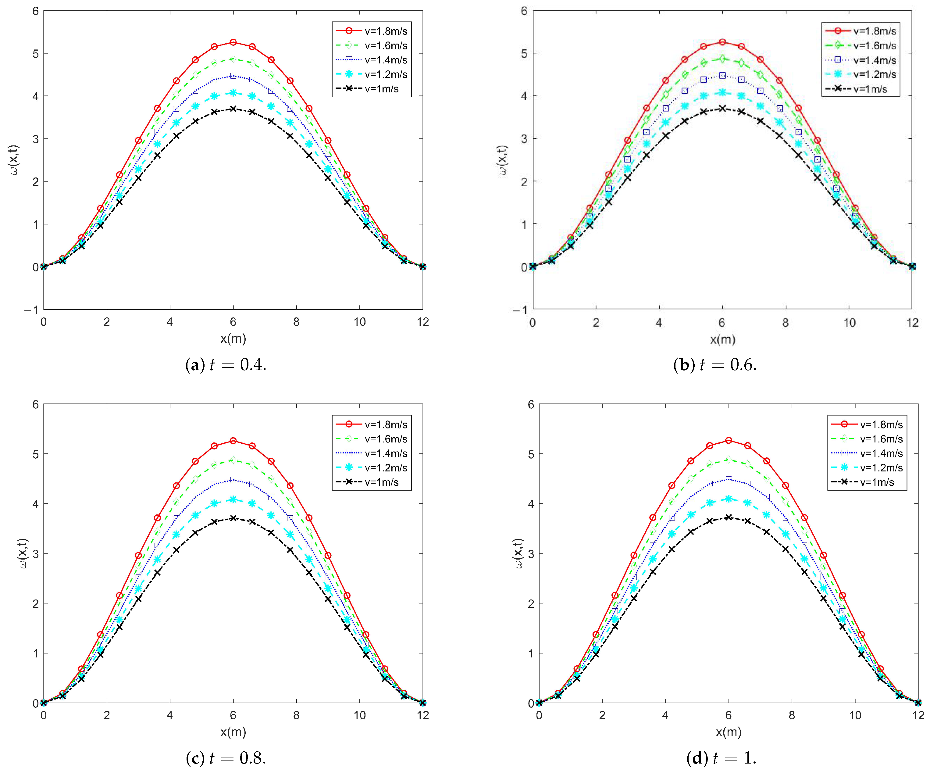
This section investigates the influence of fluid velocity on the displacement of a viscoelastic pipe. Subjected to a uniform load of f = 100 N, the viscoelastic pipe is analyzed under varying internal fluid velocities. Figure 3 presents the displacement of the pipe at four different time instances. It can be observed that the displacement progressively increases over time. Moreover, as the fluid velocity increases, the displacement of the pipe also rises, indicating the system’s sensitivity to internal flow dynamics. To better understand the relationship between fluid velocity and displacement, the detailed data is presented in Table 2.
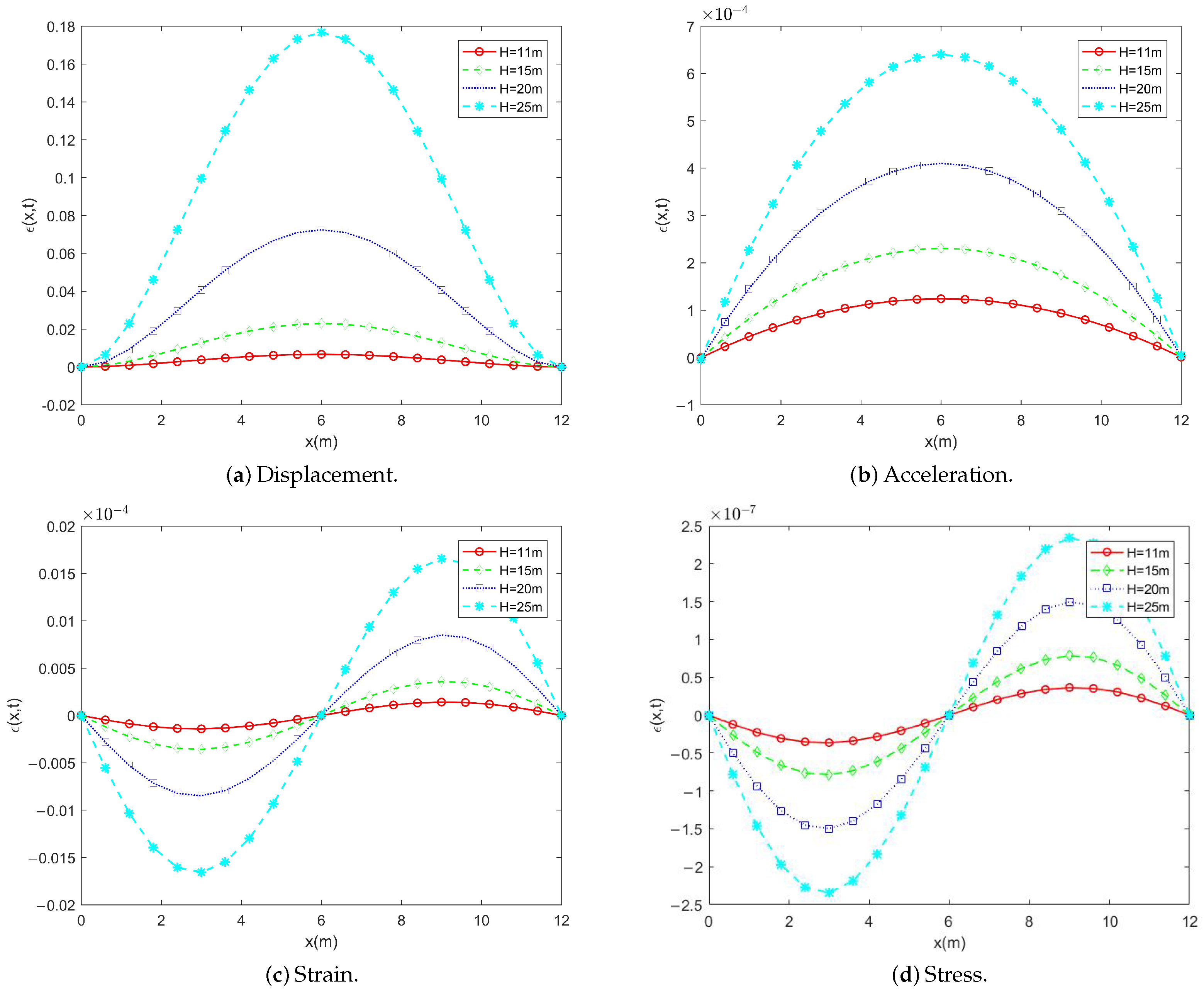
To study how pipelines of varying lengths respond during fluid transport, this section performs a numerical analysis on viscoelastic pipes with viscoelastic properties for lengths H = 11 m , 15 m , 20 m , and 25 m , under an applied load of f = 100 N , at time t = 1 s and flow velocity V = 1.1 m / s . The corresponding responses along the pipe are presented in Figure 4.
As illustrated in Figure 4a, the displacement along the pipe increases with pipe length, exhibiting pronounced nonlinear amplification and reaching peak values near the midspan. Similarly, Figure 4b shows that acceleration rises significantly as the pipe length increases with maximum values occurring near the center. The strain distribution, depicted in Figure 4c, follows a similar pattern with both magnitude and peak positions closely matching those of displacement and acceleration. Finally, Figure 4d presents the stress along the pipe, which mirrors the strain profile as the stress formulation accounting for both instantaneous strain and its historical contributions, effectively capturing the memory effect inherent in viscoelastic materials.
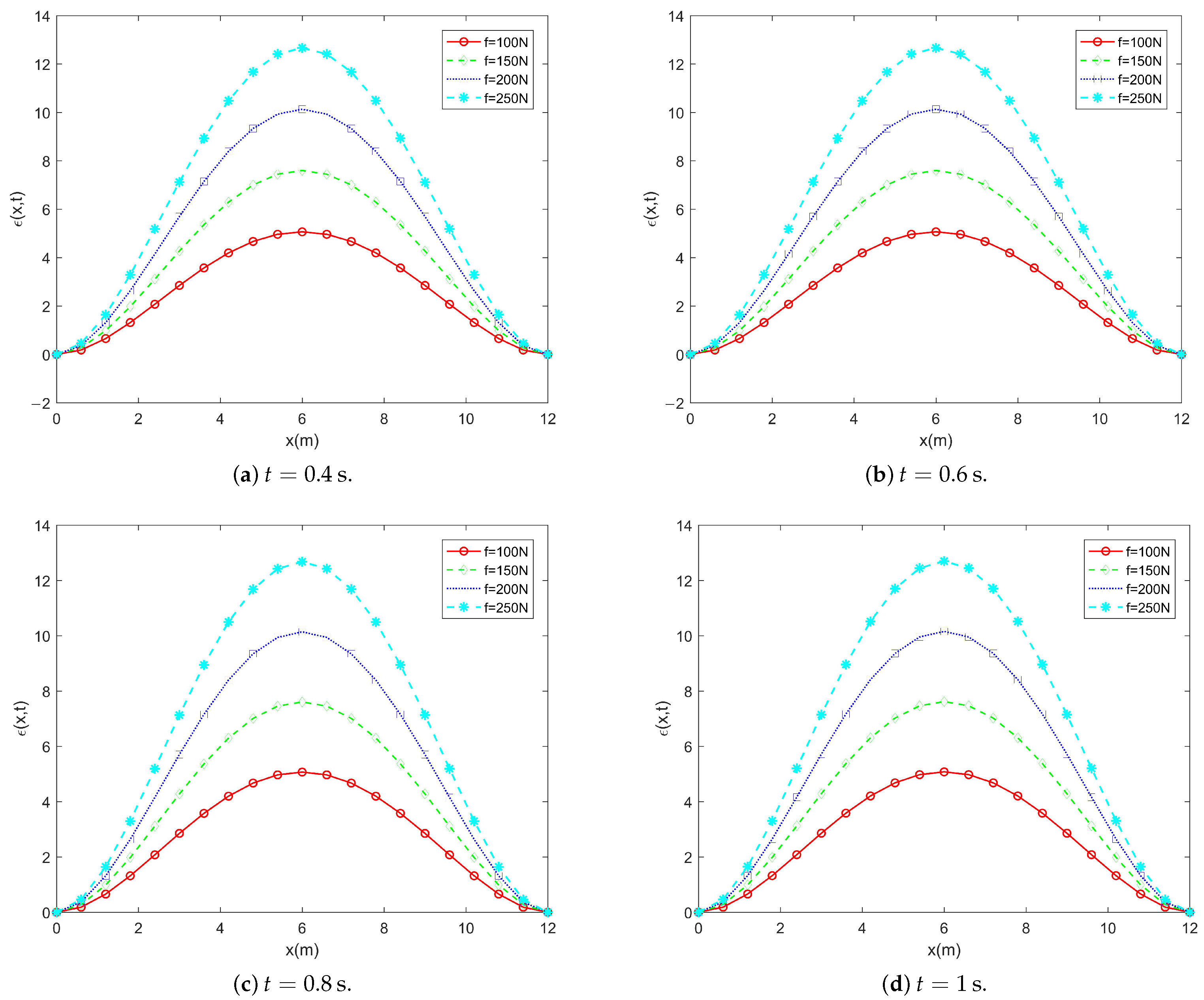
The displacement behavior of the pipe under various external loads at four different time instants ( t = 0.4 s, 0.6 s, 0.8 s, and 1 s) is illustrated in Figure 5. As the external load f increases from 100 N to 250 N, the pipe displacement becomes more significant. For a given load, the displacement also increases over time, indicating time-dependent deformation. The displacement curves exhibit a symmetric shape, with the maximum deflection occurring at the midpoint of the pipe, while both ends remain fixed. This trend reflects the viscoelastic response of the pipe under dynamic loading conditions.

8. Conclusions

In this study, we develop an efficient displacement-type Bernstein polynomial algorithm to address the governing equation with a variable fractional order for fluid-conveying viscoelastic pipes. A variable fractional-order constitutive model is established to precisely characterize the viscoelastic properties of the pipes, which is followed by a systematic analysis of their displacement responses under different parameter conditions.
The main research objectives have been successfully achieved:
  • A variable-order fractional operator matrix is constructed using shifted Bernstein polynomials, and discretization transforms the governing equation into an algebraic form suitable for computation. Combined with dimensionless formulation and dynamic analysis, the proposed method demonstrates high efficiency and accuracy in solving variable fractional-order models of viscoelastic fluid-conveying pipes.
  • Numerical results indicate that both fluid velocity and external loading significantly affect pipe displacement with increases in either factor leading to larger deformations over time. In addition, pipe length amplifies displacement, acceleration, strain, and stress in a nonlinear manner with peak responses typically occurring near the midspan.
  • The results of this study highlight the pronounced time-dependent and memory effects of viscoelastic materials, providing valuable insights into the dynamic behavior of pipes conveying fluid.
  • Future research may focus on extending the proposed Bernstein polynomial-based algorithm to more complex structures, such as multi-span or branched viscoelastic pipeline networks. Incorporating temperature-dependent or pressure-dependent fractional orders could further enhance the model’s realism. Additionally, coupling this framework with optimization techniques and experimental validation would provide a deeper understanding of the interplay between fractional-order dynamics and real-world engineering applications. The methodology can also be adapted to other fields—such as biomathematics, geophysics, and smart materials—to model systems exhibiting hereditary or memory effects under variable fractional-order behavior.

Author Contributions

Conceptualization: Z.L.; Software: Z.L.; Validation: J.Q. and Y.C. (Yiming Chen); Data curation: Z.L. and D.Y.; Writing—original draft preparation: Z.L.; Writing—review and editing: Y.C. (Yuhuan Cui) and A.Y.; Supervision: Y.C. (Yuhuan Cui); Project administration: A.Y.; Funding acquisition: A.Y. All authors have read and agreed to the published version of the manuscript.

Funding

This work is supported by the National Natural Science Foundation of China (52074126) and the Natural Science Foundation of Hebei Province (E2022209110) in China.

Data Availability Statement

The original contributions presented in this study are included in the article. Further inquiries can be directed to the corresponding author.

Conflicts of Interest

The authors confirm that there are no conflicts of interest regarding this work.

List of Abbreviations

AbbreviationFull Form
FKVFractional-order Kelvin–Voigt model
VOFCVariable-order fractional calculus
VFPDEVariable fractional partial differential equation
PINNPhysics-informed neural network
FCFractional calculus
MATLABMATLAB software
PDEPartial differential equation

References

  1. Ananthapadmanabhan, S.; Saravanan, U. Numerical techniques for solving truss problems involving viscoelastic materials. Int. J. Non-Linear Mech. 2020, 122, 103479. [Google Scholar] [CrossRef]
  2. Yun, K.S.; Youn, S.K. Microstructural topology optimization of viscoelastic materials of damped structures subjected to dynamic loads. Int. J. Solids Struct. 2018, 147, 67–79. [Google Scholar] [CrossRef]
  3. Rajabi, K.; Hosseini-Hashemi, S. On the application of viscoelastic orthotropic double-nanoplates systems as nanoscale mass-sensors via the generalized Hooke’s law for viscoelastic materials and Eringen’s nonlocal elasticity theory. Compos. Struct. 2017, 180, 105–115. [Google Scholar] [CrossRef]
  4. De Lima, A.; Rade, D.; Lacerda, H.; Araújo, C. An investigation of the self-heating phenomenon in viscoelastic materials subjected to cyclic loadings accounting for prestress. Mech. Syst. Signal Process. 2015, 58, 115–127. [Google Scholar] [CrossRef]
  5. Fang, J.; Näsholm, S.P.; Chen, W.; Holm, S. The fractional constitutive models for nonlocal material based on scattering wave equations. Mech. Time-Depend. Mater. 2022, 26, 171–193. [Google Scholar] [CrossRef]
  6. Freundlich, J. Transient vibrations of a fractional Kelvin-Voigt viscoelastic cantilever beam with a tip mass and subjected to a base excitation. J. Sound Vib. 2019, 438, 99–115. [Google Scholar] [CrossRef]
  7. Blair, G.S.; Caffyn, J. VI. An application of the theory of quasi-properties to the treatment of anomalous strain-stress relations. Lond. Edinb. Dublin Philos. Mag. J. Sci. 1949, 40, 80–94. [Google Scholar] [CrossRef]
  8. Kempfle, S.; Schäfer, I.; Beyer, H. Fractional calculus via functional calculus: Theory and applications. Nonlinear Dyn. 2002, 29, 99–127. [Google Scholar] [CrossRef]
  9. Di Paola, M.; Reddy, J.; Ruocco, E. On the application of fractional calculus for the formulation of viscoelastic Reddy beam. Meccanica 2020, 55, 1365–1378. [Google Scholar] [CrossRef]
  10. Nonnenmacher, T.; Glöckle, W. A fractional model for mechanical stress relaxation. Philos. Mag. Lett. 1991, 64, 89–93. [Google Scholar] [CrossRef]
  11. Simpson, R.; Jaques, A.; Nuñez, H.; Ramirez, C.; Almonacid, A. Fractional calculus as a mathematical tool to improve the modeling of mass transfer phenomena in food processing. Food Eng. Rev. 2013, 5, 45–55. [Google Scholar] [CrossRef]
  12. Diethelm, K.; Ford, N.J. Analysis of fractional differential equations. J. Math. Anal. Appl. 2002, 265, 229–248. [Google Scholar] [CrossRef]
  13. Taghvafard, H.; Erjaee, G. Phase and anti-phase synchronization of fractional order chaotic systems via active control. Commun. Nonlinear Sci. Numer. Simul. 2011, 16, 4079–4088. [Google Scholar] [CrossRef]
  14. Lin, Y.; Xu, C. Finite difference/spectral approximations for the time-fractional diffusion equation. J. Comput. Phys. 2007, 225, 1533–1552. [Google Scholar] [CrossRef]
  15. Farea, A.; Yli-Harja, O.; Emmert-Streib, F. Using Physics-Informed Neural Networks for Modeling Biological and Epidemiological Dynamical Systems. Mathematics 2025, 13, 1664. [Google Scholar] [CrossRef]
  16. Hu, R.; Aziz, M.H.N.; Mohamed, N.A.; Aruchunan, E. Modeling and analysis of dynamical behavior in a fractional-order COVID-19 epidemic model with media coverage: A case study of Malaysia. Alex. Eng. J. 2025, 127, 1081–1095. [Google Scholar] [CrossRef]
  17. Chen, Y.M.; Wei, Y.Q.; Liu, D.Y.; Yu, H. Numerical solution for a class of nonlinear variable order fractional differential equations with Legendre wavelets. Appl. Math. Lett. 2015, 46, 83–88. [Google Scholar] [CrossRef]
  18. Soradi-Zeid, S.; Jahanshahi, H.; Yousefpour, A.; Bekiros, S. King algorithm: A novel optimization approach based on variable-order fractional calculus with application in chaotic financial systems. Chaos Solitons Fractals 2020, 132, 109569. [Google Scholar] [CrossRef]
  19. Hassani, H.; Machado, J.T.; Naraghirad, E. An efficient numerical technique for variable order time fractional nonlinear Klein-Gordon equation. Appl. Numer. Math. 2020, 154, 260–272. [Google Scholar] [CrossRef]
  20. Hu, R.; Aruchunan, E.; Aziz, M.H.N.; Cheng, C.; Wiwatanapataphee, B. Dynamic analysis and optimal control of a fractional-order epidemic model with nucleic acid detection and individual protective awareness: A Malaysian case study. AIMS Math. 2025, 10, 16157–16199. [Google Scholar] [CrossRef]
  21. Wang, Y.; Chen, Y. Dynamic analysis of the viscoelastic pipeline conveying fluid with an improved variable fractional order model based on shifted Legendre polynomials. Fractal Fract. 2019, 3, 52. [Google Scholar] [CrossRef]
  22. Peng, G.; Xiong, Y.; Liu, L.; Gao, Y.; Wang, M.; Zhang, Z. 3-D non-linear dynamics of inclined pipe conveying fluid, supported at both ends. J. Sound Vib. 2019, 449, 405–426. [Google Scholar] [CrossRef]
  23. Chang, G.H.; Modarres-Sadeghi, Y. Flow-induced oscillations of a cantilevered pipe conveying fluid with base excitation. J. Sound Vib. 2014, 333, 4265–4280. [Google Scholar] [CrossRef]
  24. He, F.; Dai, H.; Huang, Z.; Wang, L. Nonlinear dynamics of a fluid-conveying pipe under the combined action of cross-flow and top-end excitations. Appl. Ocean. Res. 2017, 62, 199–209. [Google Scholar] [CrossRef]
  25. Rahmati, M.; Mirdamadi, H.R.; Goli, S. Divergence instability of pipes conveying fluid with uncertain flow velocity. Physica A 2018, 491, 650–665. [Google Scholar] [CrossRef]
  26. Letelier, M.F.; Siginer, D.A.; Almendra, D.L.; Stockle, J.S. Resonance in laminar pipe flow of non-linear viscoelastic fluids. Int. J. Non-Linear Mech. 2019, 115, 53–60. [Google Scholar] [CrossRef]
  27. Yang, X.; Yang, T.; Jin, J. Dynamic stability of a beam-model viscoelastic pipe for conveying pulsative fluid. Acta Mech. Solida Sin. 2007, 20, 350–356. [Google Scholar] [CrossRef]
  28. Tang, Y.; Zhen, Y.; Fang, B. Nonlinear vibration analysis of a fractional dynamic model for the viscoelastic pipe conveying fluid. Appl. Math. Model. 2018, 56, 123–136. [Google Scholar] [CrossRef]
  29. Dehrouyeh-Semnani, A.M.; Dehdashti, E.; Yazdi, M.R.H.; Nikkhah-Bahrami, M. Nonlinear thermo-resonant behavior of fluid-conveying FG pipes. Int. J. Eng. Sci. 2019, 144, 103141. [Google Scholar] [CrossRef]
  30. Carrera, Y.; Avila-de La Rosa, G.; Vernon-Carter, E.; Alvarez-Ramirez, J. A fractional-order Maxwell model for non-Newtonian fluids. Physica A 2017, 482, 276–285. [Google Scholar] [CrossRef]
  31. Ren, D.; Shen, X.; Li, C.; Cao, X. The fractional Kelvin-Voigt model for Rayleigh surface waves in viscoelastic FGM infinite half space. Mech. Res. Commun. 2018, 87, 53–58. [Google Scholar] [CrossRef]
  32. Lewandowski, R.; Wielentejczyk, P. Nonlinear vibration of viscoelastic beams described using fractional order derivatives. J. Sound Vib. 2017, 399, 228–243. [Google Scholar] [CrossRef]
  33. Xu, H.; Jiang, X. Creep constitutive models for viscoelastic materials based on fractional derivatives. Comput. Math. Appl. 2017, 73, 1377–1384. [Google Scholar] [CrossRef]
  34. Heymans, N.; Podlubny, I. Physical interpretation of initial conditions for fractional differential equations with Riemann-Liouville fractional derivatives. Rheol. Acta 2006, 45, 765–771. [Google Scholar] [CrossRef]
  35. Magin, R.L. Fractional calculus models of complex dynamics in biological tissues. Comput. Math. Appl. 2010, 59, 1586–1593. [Google Scholar] [CrossRef]
  36. Joseph, D.; Ramachandran, R.; Alzabut, J.; Jose, S.A.; Khan, H. A fractional-order density-dependent mathematical model to find the better strain of wolbachia. Symmetry 2023, 15, 845. [Google Scholar] [CrossRef]
  37. Cui, Y.; Qu, J.; Han, C.; Cheng, G.; Zhang, W.; Chen, Y. Shifted Bernstein–Legendre polynomial collocation algorithm for numerical analysis of viscoelastic Euler–Bernoulli beam with variable order fractional model. Math. Comput. Simul. 2022, 200, 361–376. [Google Scholar] [CrossRef]
  38. Gadomski, A.; Rubí, J.; Łuczka, J.; Ausloos, M. On temperature-and space-dimension dependent matter agglomerations in a mature growing stage. Chem. Phys. 2005, 310, 153–161. [Google Scholar] [CrossRef]
  39. Feng, Y.; Liu, L.; Chen, Y. Numerical analysis of fractional-order variable section cantilever beams. ICIC Express Lett. 2019, 13, 547–555. [Google Scholar]
  40. Sazesh, S.; Shams, S. Vibration analysis of cantilever pipe conveying fluid under distributed random excitation. J. Fluids Struct. 2019, 87, 84–101. [Google Scholar] [CrossRef]
  41. Wang, L.; Chen, Y.M. Shifted-Chebyshev-polynomial-based numerical algorithm for fractional order polymer visco-elastic rotating beam. Chaos Solitons Fractals 2020, 132, 109585. [Google Scholar] [CrossRef]
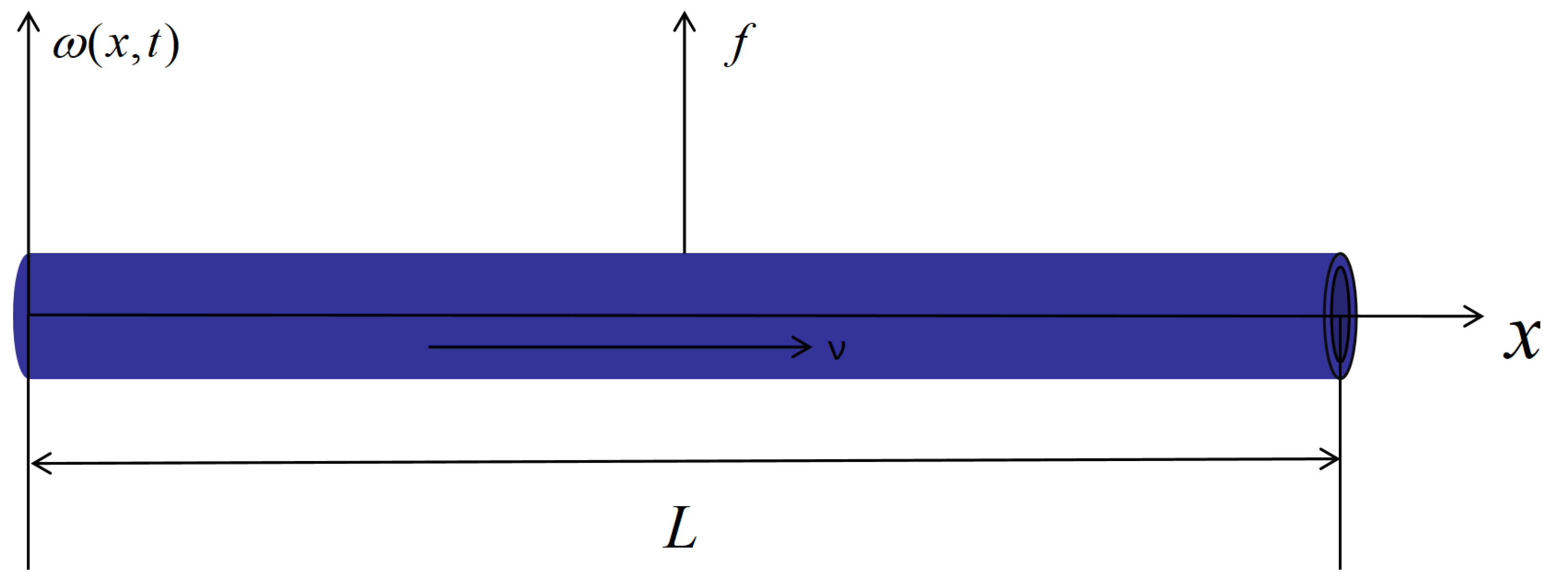
Figure 1. Viscoelastic channel configuration.
Fractalfract 09 00747 g001
Figure 2. Exact and numerical solutions evaluated at various points.
Fractalfract 09 00747 g002
Figure 3. Displacements of pipe under external load f = 100 N at different fluid velocities.
Fractalfract 09 00747 g003
Figure 4. Time-dependent dynamic responses of viscoelastic fluid-conveying pipes at various lengths for n = 5 , including displacement, acceleration, strain, and stress ( f = 100 N, t = 1 s, V = 1.1 m/s).
Fractalfract 09 00747 g004
Figure 5. Pipe displacement responses at different time instants under varying external loading conditions.
Fractalfract 09 00747 g005
Table 1. The absolute error e ( x , t ) corresponding to the numerical example with n = 5 .
e(x,t) t = 0.2 t = 0.4 t = 0.6 t = 0.8
x = 0.2 2.795 × 10 12 2.502 × 10 12 5.097 × 10 12 1.081 × 10 12
x = 0.4 3.307 × 10 12 2.175 × 10 12 5.247 × 10 12 8.684 × 10 12
x = 0.6 4.637 × 10 12 1.303 × 10 12 4.682 × 10 12 6.792 × 10 12
x = 0.8 6.229 × 10 12 4.661 × 10 12 3.645 × 10 12 5.706 × 10 12
Table 2. Physical parameter values of pipe.
NotationNameValueDimension
IArea moment of inertia0.0001798m4
MFluid quality11.74416kg
mPipe quality289.00198kg
vFluid velocity1.1m/s
LLength of the pipe11m
cDamping ratio0.81
Disclaimer/Publisher’s Note: The statements, opinions and data contained in all publications are solely those of the individual author(s) and contributor(s) and not of MDPI and/or the editor(s). MDPI and/or the editor(s) disclaim responsibility for any injury to people or property resulting from any ideas, methods, instructions or products referred to in the content.