Crop and Weed Segmentation and Fractal Dimension Estimation Using Small Training Data in Heterogeneous Data Environment

Abstract

The segmentation of crops and weeds from camera-captured images is a demanding research area for advancing agricultural and smart farming systems. Previously, the segmentation of crops and weeds was conducted within a homogeneous data environment where training and testing data were from the same database. However, in the real-world application of advancing agricultural and smart farming systems, it is often the case of a heterogeneous data environment where a system trained with one database should be used for testing with a different database without additional training. This study pioneers the use of heterogeneous data for crop and weed segmentation, addressing the issue of degraded accuracy. Through adjusting the mean and standard deviation, we minimize the variability in pixel value and contrast, enhancing segmentation robustness. Unlike previous methods relying on extensive training data, our approach achieves real-world applicability with just one training sample for deep learning-based semantic segmentation. Moreover, we seamlessly integrated a method for estimating fractal dimensions into our system, incorporating it as an end-to-end task to provide important information on the distributional characteristics of crops and weeds. We evaluated our framework using the BoniRob dataset and the CWFID. When trained with the BoniRob dataset and tested with the CWFID, we obtained a mean intersection of union (mIoU) of 62% and an F1-score of 75.2%. Furthermore, when trained with the CWFID and tested with the BoniRob dataset, we obtained an mIoU of 63.7% and an F1-score of 74.3%. We confirmed that these values are higher than those obtained by state-of-the-art methods.

1. Introduction

Expanding crop efficiency is becoming increasingly important as food security concerns are increasing globally. However, it faces many challenges, such as a lack of manpower, uncertain environmental conditions, soil factors, and scarcity of water. To achieve high yields and address such problems, previous research used plant phenotyping methods and monitoring systems to strengthen crop productivity in precision agriculture [1,2]. Over time, traditional farming has shifted toward modern automated farming to increase yields and minimize labor costs, individual effort, and time.

Image processing has been widely adopted in various fields [3,4,5,6,7,8,9,10,11]. In addition, recently, deep learning methods have offered various solutions, and the use of computer vision has grown significantly in various applications including building monitoring, image enhancement, medical image processing, biomedical engineering, and underwater computer vision, where some research has adopted fractal-related perspectives, also in [9,10,11,12,13,14,15,16]. Although the studies adopt similar concepts of fractal dimension (FD) estimations [12,13,15], their applications are different in terms of building monitoring and medical image processing. Semantic segmentation also exhibits a fundamental role in the accurate recognition of crops and weeds [17,18]. Two mainstream methods exist for crop and weed detection. The first is box-based detection [19,20]; however, it has the drawback of overlooking specific regions in weeds and crops. The second type is semantic segmentation or pixel-based detection [21,22,23], which detects precise regions of weeds or crops at the pixel level. Therefore, correctly identifying the crop and weed segments is essential. Crop and weed segments typically have irregular shapes, and training with these irregularly shaped segments comes with an imbalance in the data. The irregular shapes of “sugar beets” (BoniRob) [24] and crop/weed field image datasets (CWFIDs) [25] are shown in Figure 1. A considerable amount of data is usually required during training, particularly in segmentation cases. To acquire more data, it may be necessary for experts to create a large number of annotations, which would require considerable time and effort. In some scenarios, if a considerable amount of training data are unavailable, the testing performance decreases. To avoid such a drop in performance owing to insufficient training data, a method using small amounts of training data was proposed by Nguyen et al. [26], which also achieved good performance. Homogenous data usually show satisfactory results; however, when applied to heterogeneous environments, where the testing and training datasets are completely different, the overall results decrease significantly. Abdalla et al. [27] showed that the efficacy of these algorithms is compromised in complex environments due to their heavy reliance on various factors, including lighting conditions and weed density, for feature extraction. Thus, it is essential to propose an effective and reliable framework that segments crops and weeds accurately, even in complex heterogeneous environments.

Figure 1. Sample images (left) and ground-truth masks (right) for crops (white pixels) and weeds (gray pixels) in BoniRob dataset (upper) and CWFID (lower).

To solve these issues, we propose an approach for weed and crop segmentation and fractal dimension estimation using a small amount of training data in a heterogeneous data environment. The contributions of this study include the following:

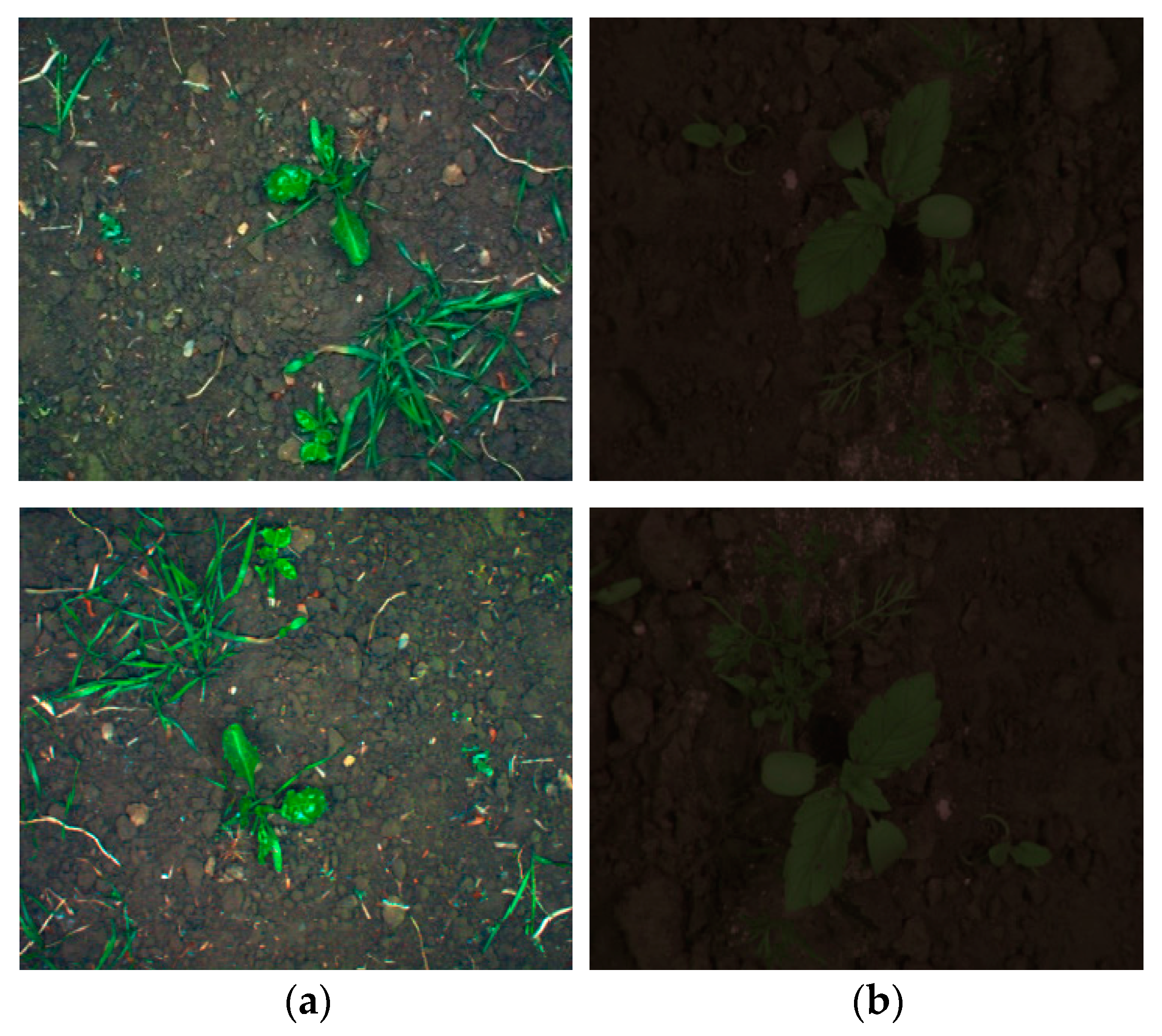
• This is the first study that considers the segmentation of crops and weeds within a heterogeneous environmental setup utilizing one training data sample. We rigorously investigate the factors that cause performance degradation in heterogeneous datasets, including variations in illumination and contrast. To address this problem, we propose a method that applies the Reinhard (RH) transformation, leveraging the mean and standard deviation (std) adjustments.
• We address the issue of high data availability for real-world applications. For this purpose, we improved the performance using a small amount of training data. The small amount of additional training data significantly improves the segmentation performance while requiring fewer computational resources and less training time.
• We introduce the FD estimation approach in our framework, which is seamlessly combined as an end-to-end task to provide important information on the distributional features of crops and weeds.
• It is noteworthy that our proposed framework [28] is publicly accessible for a fair comparison with other studies.

The structure of the remaining sections of this study is as follows: Multiple related studies are described in Section 2. In Section 3, we outline the proposed approach. Section 4 describes a comparison between the proposed framework and the state-of-the-art (SOTA) methods in terms of their performance. Section 5 presents a discussion, while Section 6 presents the conclusion and outlines future work.

2. Related Work

We classified previous studies on crop and weed segmentation into homogenous data-based methods and heterogeneous data-based methods as follows.

2.1. Homogenous Data-Based Methods

Homogeneous data-based methods mostly exhibit high accuracy because their training and testing data distributions originate from the same dataset. Many related studies using homogenous data have been conducted to date, and they have been highly effective in multiple domains, not only in agriculture. In general, the term “a large amount of training data” is used extensively in the literature. Typically, a considerable amount of training data is needed to efficiently train the model and achieve higher accuracy. Many prior studies have been conducted using a large amount of training data. Furthermore, learning-based methods are grouped into two main groups: the handcrafted feature-based and the deep learning-based methods.

2.1.1. Handcrafted Feature-Based Methods

Before the significant advancements in deep learning, features were often manually engineered, referred to as manual or handcrafted features, as they were developed progressively. In [29], a random forest classifier (RFC) is used to handle the overlap of together-grown different crops and weed plants. A Markov random field was also applied to smooth the sparse pixels. Another study by Lottes et al. [30] used the same RFC for vegetation detection using local and object-based features. Lottes et al. [31] used unmanned aerial vehicles (UAVs) and various robots to monitor weeds and crops. They implemented and evaluated plant-tailored feature extraction. Many systems rely on these techniques, primarily because they require fewer computations and have shorter execution times.

2.1.2. Deep Feature-Based Methods

Deep learning techniques utilizing deep features are advancing to automate precision agriculture [32], particularly by making intelligent decisions in the semantic segmentation of crops and weeds. Pixelwise classification networks play a crucial role in detecting objects and properly delimiting their boundaries so that automated robotic weeders can perform precision spraying and weeding operations. Commonly used base networks in semantic segmentation studies include DeepLab [33], fully convolutional networks [34], U-Net [35], and SegNet [36]. These networks, along with certain blocks proposed in various studies, employ an encoder–decoder architecture for crop and weed segmentation. The encoder architecture transforms input data into a compressed representation capturing their key features, while the decoder module upsamples and restores the spatial features of areas where the edges of objects are absent. The base U-Net encoder–decoder network has undergone modifications into multiple architectures, as seen in the work by Zou et al. [37]. They achieved this by reducing feature extraction in the encoder and adding a skip connection at the output layer to recover object details, thereby enhancing model accuracy. They conducted two-stage training to accurately segment weeds and showcased greater applicability in the field. However, the robustness of these models has not been tested using heterogeneous datasets.

Milioto et al. [38] designed an end-to-end model identical to the previously used encoder–decoder format. This network is narrow and fast; however, the dataset used here covers a very small portion of crops and weeds. The model was developed by modifying Enet [39] and SegNet [36] through the replacement of convolutional (Conv) layers with residual blocks. Fathipoor et al. [40], based on an encoder–decoder in U-Net and U-Net++ [41] architectures, demonstrated promising overall results for weed segmentation in the early stages. In a prior study [18], a two-stage approach named MTS-CNN was proposed to segment crops and weeds utilizing U-Net with a visual geometry group (VGG)-16 [42]. The model separates object segmentation from crop and weed segmentation in two stages to enhance accuracy, also creating a loss function to address the class imbalance problem of the crop and weed dataset. However, errors made by the first model can impact overall model performance, and training takes a considerable amount of time. Another study [43] relied on images captured by different cameras mounted on an unmanned aerial vehicle (UAV) for crop and weed segmentation. The authors used a modified VGG-16 encoder and modified U-Net decoder architecture, concatenating images of different formats into channel directions to improve segmentation accuracy. Alongside recent developments in deep convolutional neural networks (CNNs), several new networks have been designed to enhance crop and weed segmentation. Dilated convolution [44] and atrous convolution [33] were integrated into the network alongside a universal function approximation block (UFAB) [45] to improve segmentation. However, these networks require inputs of near-infrared (NIR) light and red, green, and blue (RGB) channels that are unavailable in real time. Wang et al. [46] devised a dual attention network (DA-Net) bridging the gap between low- and high-level featured data using branch and spatial attention. The employed self-attention is computationally demanding due to the size of the spatial features. Siddiqui et al. [47] explored data augmentation (DA) using CNN methods to distinguish weeds from crops. In another study, Khan et al. [48] introduced a new cascaded encoder–decoder network (CED-Net) modifying the base network U-Net into four stages to distinguish between weeds and crops. The inclusion of stages in the network enhanced crop and weed segmentation accuracy. From the above discussion, we can conclude that these deep learning-based methods offer greater accuracy than handcrafted feature-based methods. However, all prior studies were conducted in a homogeneous data environment, where training and testing were performed using the same dataset.

2.2. Heterogeneous Data-Based Methods

Previous studies on crop and weed segmentation have not explored the use of heterogeneous data, where training and testing are conducted using different datasets. However, a model trained with the first dataset is often applied to the second dataset without intensive training using the second dataset. Additionally, sufficient training data cannot often be acquired for real-world applications. However, no previous studies have considered insufficient training data for crop or weed segmentation. Therefore, we propose a framework for weed and crop segmentation and FD estimation utilizing limited training data in a heterogeneous data environment. The strengths and weaknesses of the proposed framework for crop and weed segmentation relative to other techniques are listed in Table 1.

Table 1. Comparisons of proposed method with previous ones on crop and weed segmentation.

Data	Type	Method	Strength/Motivation	Weakness
Homogeneous data-based	Handcrafted feature-based	RFC [29]	Handling overlapping of crops and weeds	Overlapping of multiple plants with the same class cannot be split
		RFC + vegetation detection [30]	Detection of local and object-based features	Smoothing as post-processing on only local features
		Plant-tailored feature extraction [31]	UAV intra-row-space-based weed detection in challenging conditions	The number of weeds is much smaller in the datasets used
	Deep feature-based	MTS-CNN [18]	Separate object segmentation to avoid background-biased learning	Dependency of first stage network on second stage network
		Modified U-Net [37]	Effective two-stage training method with large applicability	Only weed-targeted segmentation
		SegNet + Enet [38]	Fast and more accurate pixelwise predictions	Images contain very small portions of crops and weeds
		U-Net and U-Net++ [40]	Detecting weeds in the early stages of growth	Uses a very small dataset and has no suitable real-time application
		Modified U-Net + modified VGG-16 [43]	Effective result for distribution estimation problem with graphics processing unit (GPU)-based embedded board	Not focusing on the exact location of weeds in the images
		UFAB [45]	Reducing redundancy by strengthening the model diversity	Unavailability of RGB and NIR input
		DA-Net [46]	Expanding receptive field without affecting the computational cost	Hard and time-consuming mechanism to parallelize the system using attention modules
		4-layered CNN + data augmentation [47]	Good for the early detection of weeds, improving production, and is easy to deploy because of the cheap cost	Minimizing accuracy if weeds are not detected at the early stages
		CED-Net [48]	Using a light model and achieving efficient results	Error at any level among the four levels affects the overall performance
Heterogeneous data-based		Proposed framework (proposed)	Use of small training images in a heterogeneous environment	Preprocessing steps are included

3. Proposed Method

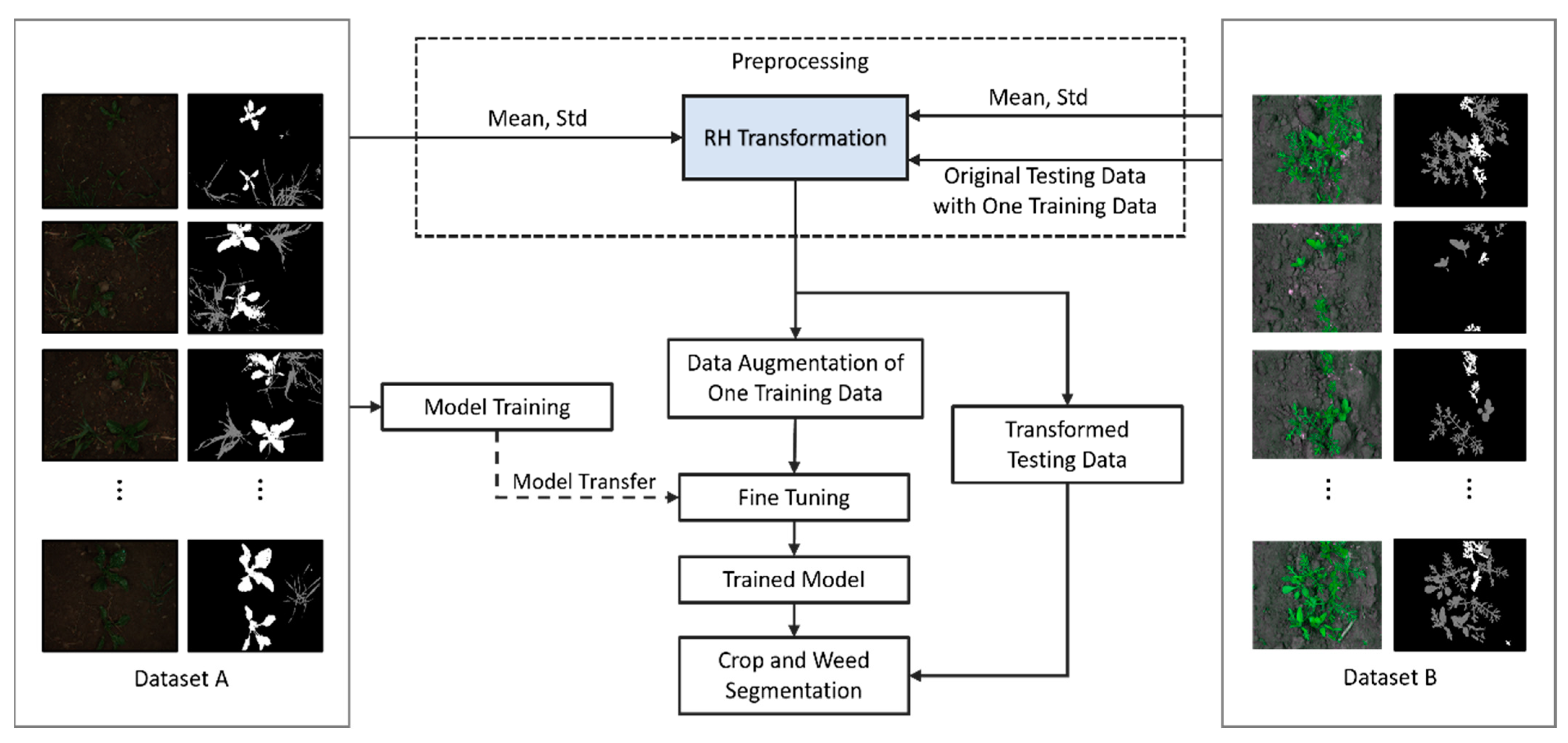
3.1. Overview of Proposed Method

Figure 2 depicts an overview of the flow of our framework. During training, we train the conventional semantic segmentation model with Dataset A. Next, we preprocess the images of Dataset B using the RH transformation, which is based on the mean and std of Datasets A and B. This transformation adjusts the visual properties of the images, such as intensity, illumination, and contrast, to make them similar to the reference image in a heterogeneous environment. Then, we select one training data from the preprocessed Dataset B and perform DA on it to augment the training data. Afterward, we perform fine-tuning and train the model from scratch with Dataset A using the augmented data, and we perform the semantic segmentation of weeds and crops utilizing the testing data from Dataset B.

Figure 2. Overview of the proposed framework flow.

3.2. Preprocessing

3.2.1. RH Transformation

Many factors such as variations in intensity, illumination, and contrast cause performance degradation, particularly in heterogeneous environments. Transferring colors from one image (reference) to another (target) is a significant problem, particularly when the color information in the reference image does not match the newly generated image, causing quality and performance degradation. To address performance degradation using heterogeneous data, we adopted the RH transformation [49] with average mean and std adjustments to enhance the visual attributes of the images. Many prior transformation methods and color spaces enhance the visual characteristics of an image. In the Ɩαβ color space (LCS) [50], “Ɩ” indicates a brightness channel that captures the brightness independently of color attributes, the “α” channel encapsulates yellow and blue hues, and the “β” channel encloses the interplay between red and green shades. In the RH transformation, the LCS is used. The LCS minimizes the relative significance of each weight, with a matrix proposed for converting vectors from RGB to LCS. The RH transformation changes the mean and std values of the color channels based on the LCS that consistently represents the pixel colors in an image. As shown in Equation (1), it uses the $\mathrm{ƒ}$ mapping function with $\delta$ parameters to transform the $dataB$ into preprocessed $dataB’$.

$$dataB’=\mathrm{ƒ}(dataB,\delta )$$

(1)

For the transformation, the RGB images are manipulated in the LCS and then transformed into the long, medium, short (LMS) cone space, and the logarithmic of the LMS space is obtained to reduce skewness [49]. The mean and std for all the axes in the LCS are separately calculated to make images more synthetic. Moreover, the color space is normalized by subtracting the mean of the data points from the original data point value, as follows:

$${\mathrm{Ɩ}}^{^}=\mathrm{Ɩ}-{Ɩ}_m,$$

(2)

$${\alpha }^{^}=\alpha -{\alpha }_m,$$

(3)

$${\beta }^{^}=\beta -{\beta }_m$$

(4)

where ${Ɩ}_m,{\alpha }_m,{\beta }_m$ denote the average mean data point values of the $\mathrm{Ɩ},\alpha ,\mathrm{a}\mathrm{n}\mathrm{d}\beta$ data points, and ${\mathrm{Ɩ}}^{^},{\alpha }^{^},\mathrm{a}\mathrm{n}\mathrm{d}{\beta }^{^}$ show the normalized space data points. Upon normalizing the space, data points are scaled by std ${\sigma }_j^{Ɩ}{,\sigma }_j^{\alpha }{,\sigma }_j^{\beta }$ for the reference images and ${\sigma }_i^{Ɩ}{,\sigma }_i^{\alpha }{,\sigma }_i^{\beta }$ for the target images. Finally, ${Ɩ}^{°}{,\alpha }^{°}{,\beta }^{°}$ are the scaled points for the transformed images, as follows:

$${Ɩ}^{°}=\frac{{\sigma }_i^{Ɩ}}{{\sigma }_j^{Ɩ}}{Ɩ}^{^},$$

(5)

$${\mathsf{\alpha }}^{°}=\frac{{\sigma }_i^{\alpha }}{{\sigma }_j^{\alpha }}{\mathsf{\alpha }}^{^},$$

(6)

$${\beta }^{°}=\frac{{\sigma }_i^{\beta }}{{\sigma }_j^{\beta }}{\beta }^{^}$$

(7)

The pseudo-code of the RH transformation is provided in Algorithm 1.

Algorithm 1: RH transformation with pseudo-code

Input: {dataB} tn; The total of t data samples, dataB: input dataset B images dataAm: training data from dataset A.

Output: (dataB’) the preprocessed sample

1:  Compute the std of the dataset B (input images) by    dataB _std = std (dataB (:, :))

2:  Compute the mean of the dataB    dataB _mean = mean (dataB (:, :))

3:  Compute the average std of the training data from dataset A using    dataA_std = avg (std (dataAm (:, :))

4:  Compute the average mean of the training data from dataset A using    dataA_mean = avg (mean (dataAm (:, :))

5:  Apply the RH transformation    for m = 1: x     for n = 1: y      dataB’ (m, n) = [(dataB (m, n) − dataB_mean) ×      (dataA_std/dataB_std)] + dataA_mean     end    end    return dataB’

Histograms of the RGB color channel distribution for the reference, target, and newly transformed images are shown in Figure 3a–c, respectively. The reference image is from Dataset A, the target image is from Dataset B, and the RH-transformed image is a new image generated by RH transformation. In Figure 3b, the histograms show only two channels; apparently, the red and blue channels overlap because they are replicas of each other [25]. The histogram shows the pixel values on the x-axis and the probability distribution of the pixels on the y-axis. As shown in Figure 3c, the histogram of the target image is more akin to that of the reference image in Figure 3a by RH transformation than to that of the target image in Figure 3b before RH transformation.

Figure 3. Sample histograms of (a) referenced image, (b) targeted image, (c) RH-transformed image, and (d) RH-transformed image with additional adjustment.

3.2.2. RH Transformation with Additional Adjustments

However, despite the RH transformation, there is still a difference in the relative probability distribution of each channel in Figure 3a,c. Therefore, we introduce an additional adjustment to obtain the relative probability distribution of each channel of the RH-transformed image that is more similar to that of the reference image as follows:

$${{\mathrm{m}\mathrm{i}\mathrm{n}}_{\mathrm{s}\mathrm{e}\mathrm{l}\mathrm{e}\mathrm{c}\mathrm{t}{\mathrm{p}}_{\mathrm{i}\mathrm{o}\mathrm{p}\mathrm{t}}}\left(R_t-\left(R_r-p_i\right)\right)}^2,$$

(8)

$${{\mathrm{m}\mathrm{i}\mathrm{n}}_{\mathrm{s}\mathrm{e}\mathrm{l}\mathrm{e}\mathrm{c}\mathrm{t}{\mathrm{q}}_{\mathrm{i}\mathrm{o}\mathrm{p}\mathrm{t}}}\left(G_t-\left(G_r-q_i\right)\right)}^2,$$

(9)

$${{\mathrm{m}\mathrm{i}\mathrm{n}}_{\mathrm{s}\mathrm{e}\mathrm{l}\mathrm{e}\mathrm{c}\mathrm{t}{\mathrm{r}}_{\mathrm{i}\mathrm{o}\mathrm{p}\mathrm{t}}}\left(B_t-\left(B_r-r_i\right)\right)}^2$$

(10)

where $R_t,G_t,\mathrm{a}\mathrm{n}\mathrm{d}{B}_t$ represent the pixels in the target image, and $R_r,G_r,{\mathrm{a}\mathrm{n}\mathrm{d}B}_r$ represent the pixels in the reference image. Moreover, $p_{iopt},q_{iopt},\mathrm{a}\mathrm{n}\mathrm{d}{r}_{iopt}$ are the optimal values generated by varying the $p_i,q_i,\mathrm{a}\mathrm{n}\mathrm{d}{r}_i$ values, respectively, to minimize the distance between the corresponding red, green, and blue channel distributions. To obtain this channel distribution, the following additional adjustments were made:

$${Ɩ}_{adj}={Ɩ}_m-p_{iopt},$$

(11)

$${\alpha }_{adj}={\alpha }_m-q_{iopt},$$

(12)

$${\beta }_{adj}={\beta }_m-r_{iopt}$$

(13)

where ${Ɩ}_m,{\alpha }_m,{\mathrm{a}\mathrm{n}\mathrm{d}\beta }_m$ represent the average mean data point values, and $p_{iopt},q_{iopt},\mathrm{a}\mathrm{n}\mathrm{d}{r}_{iopt}$ represent the values that make the channel distribution look more similar among the reference and transformed images. These $p_{iopt},q_{iopt},r_{iopt}$ values are subtracted from the average mean values to adjust the ${Ɩ}_{adj},$ ${\alpha }_{adj},\mathrm{a}\mathrm{n}\mathrm{d}{\beta }_{adj}$ data points. Furthermore, the transformation with additional adjustments is as follows:

$${\mathrm{Ɩ}}^{”}=\mathrm{Ɩ}-{Ɩ}_{adj},$$

(14)

$${\alpha }^{”}=\alpha -{\alpha }_{adj},$$

(15)

$${\beta }^{”}=\beta -{\beta }_{adj}$$

(16)

where ${Ɩ}_{adj},{\alpha }_{adj},and{\beta }_{adj}$ are the different data point values for additional adjustments, which are experimentally chosen to make the channel distribution similar to the reference image. These values are subtracted from the $\mathrm{Ɩ},\alpha ,\beta$ data points, and the result is ${\mathrm{Ɩ}}^{”},{\alpha }^{”},{\mathrm{a}\mathrm{n}\mathrm{d}\beta }^{”}$, which shows the normalized space data points. The newly generated histograms are visually presented in Figure 3d. As demonstrated in Figure 3d, the channel distributions resulting from the RH transformation with additional adjustments closely resemble those of the reference image in Figure 3a, in contrast to the RH without additional adjustment in Figure 3c.

Figure 4 illustrates the sample images of the referenced image, targeted image, RH-transformed image, and RH-transformed image with additional adjustments from the BoniRob dataset and CWFID.

Figure 4. Sample images of the BoniRob dataset (upper images) and CWFID (lower images). (a) Referenced image, (b) targeted image, (c) RH-transformed image, and (d) RH-transformed image with additional adjustments.

3.3. Data Augmentation of One Training Data

Data augmentation (DA) involves employing various transformations on existing data to expand and diversify a training dataset artificially. In image datasets, DA can involve procedures such as in-plane rotation, flipping, zooming, and modifying the contrast and brightness levels of the images within the training dataset [51]. The purpose behind DA is to enhance the capacity of a model to generalize and perform effectively on novel and unseen data by exposing it to a broader spectrum of variations that may be encountered in real-world contexts. We randomly selected a single image from the training data and augmented it for training. By adding augmentation to this small training dataset, we improved the segmentation performance while reducing the training time. A simple 180-degree in-plane rotation was used for DA, as depicted in Figure 5.

Figure 5. Sample training image (upper) and augmented image (lower) for training. (a) BoniRob dataset (left images) and (b) CWFID (right images).

3.4. Semantic Segmentation Networks

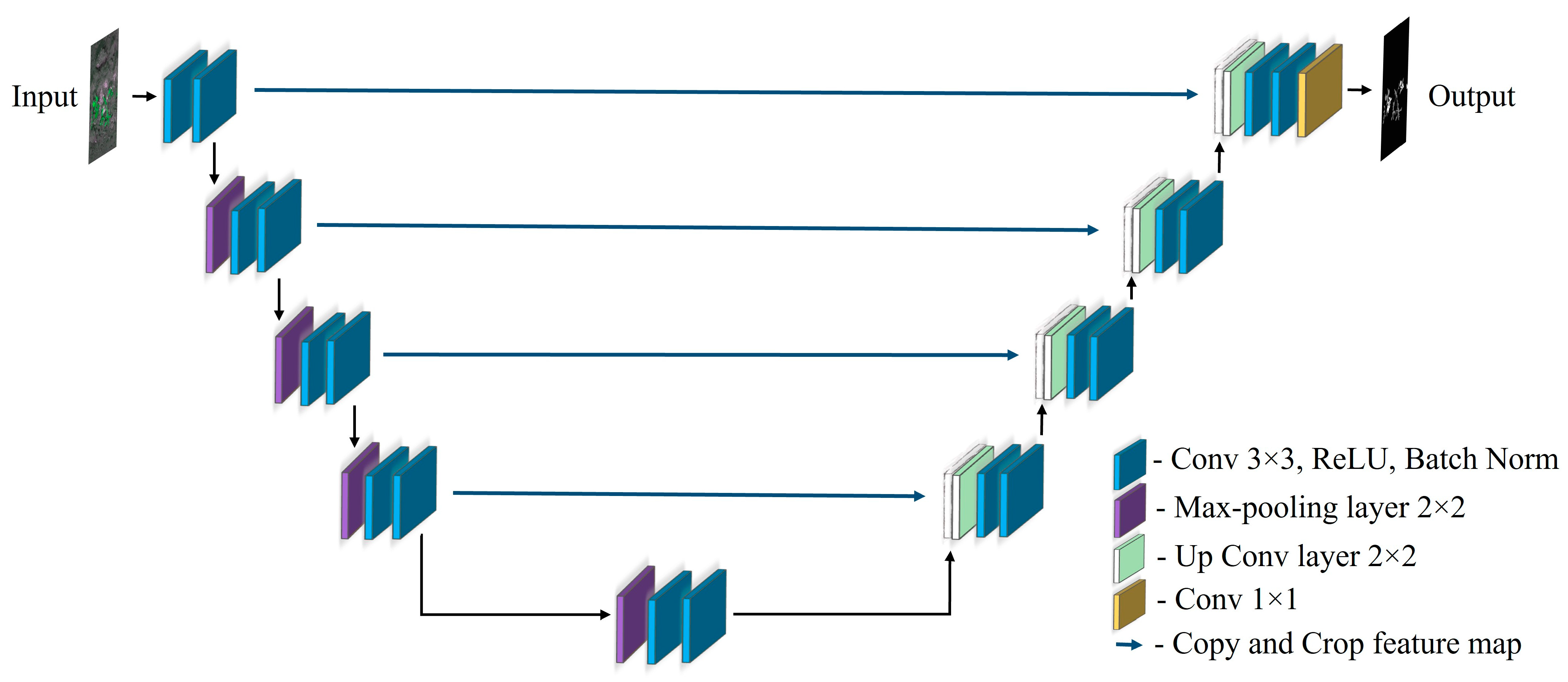
For the semantic segmentation of weeds and crops, the following conventional semantic segmentation models were adopted:

3.4.1. U-Net

U-Net [35] features a fully CNN with a U-shaped encoder–decoder framework. The input image of the encoder and the output image of the decoder have the same image size. The decoder is more or less symmetric than the encoder, and the encoder has a large feature channel for propagating contextual information to the high-resolution layer. The architecture includes two 3 × 3 Conv layers, each accompanied by a max-pooling (MP) layer of 2 × 2 kernel size, with stride 2, and a ReLU [52]. In the decoder, the tensor map was upsampled using a 2 × 2 up-convolution and concatenated with the encoder features. A final layer of 1 × 1 convolution was incorporated into the U-Net network. Figure 6 illustrates its architecture. Furthermore, the first stages of the encoder (including and before the first max-pooling layer as ${Encoder}_1$) and decoder (first up Conv layer with subsequent layers having the same spatial dimensions as ${Decoder}_1$) of the U-Net shown in Figure 6 are mathematically represented as follows:

$${Encoder}_1={\mathrm{P}}_1\left(C_1\right)where\left\{\begin{array}{c}{C}_1=Conv\left(\mathrm{C}\mathrm{o}\mathrm{n}\mathrm{v}\left(X,W_1\right)\right),\\ P_1=Maxpool\left(C_1\right)\end{array}\right.$$

(17)

$${Decoder}_1={\mathrm{C}\mathrm{R}}_1\left({\mathrm{C}}_{\mathrm{c}\mathrm{o}\mathrm{n}\mathrm{c}\mathrm{a}\mathrm{t}1}\left({\mathrm{C}}_{\mathrm{c}\mathrm{r}\mathrm{o}\mathrm{p}1}\left(U_1\right)\right)\right),$$

(18)

$$where\left\{\begin{array}{c}{U}_1=Upconv\left(B,W_{up1}\right),\\ C_{crop1}=Crop\left(R,size\left(U_1\right)\right),\\ C_{concat1}=Concatenation\left(U_1,C_{crop1}\right),\\ {CR}_1=Conv\left(\mathrm{C}\mathrm{o}\mathrm{n}\mathrm{v}\left(C_{concat1},W_{conv}\right)\right)\end{array}\right.$$

In ${Encoder}_1$, $X$ represents the input feature, and $W_1$ indicates the weight tensor for convolution operations. In every convolution operation for both the encoder and decoder, ReLU activation functions and batch normalization are applied. In ${Decoder}_1$, $B$ represents the tensor of the previous layer, and $W_{up1}$ in $\mathrm{U}\mathrm{p}\mathrm{c}\mathrm{o}\mathrm{n}\mathrm{v}\left({B,W}_{up1}\right)$ shows the weight tensor with an up-convolution operation. $R$ in $\mathrm{C}\mathrm{r}\mathrm{o}\mathrm{p}\left({R,size(U}_1)\right)$ indicates the input image size after convolutions from the encoder side with the same size as $U_1$, which is a result of the previous up-convolution. $C_{concat1}$ represents the concatenation of $U_1$ and $C_{crop1}$ which are the final calculations for the previous layers. $W_{Conv}$ represents weight tensors with convolution operations. Finally, after the convolution in the decoder, it is fed to ${CR}_1$, and the subsequent levels of decoder operations continue in a similar manner.

Figure 6. U-Net architecture.

3.4.2. Modified U-Net

Modified U-Net [37] is an updated variant of the U-Net, featuring an encoder–decoder framework. Like U-Net, the modified version includes two 3 × 3 Conv layers, each accompanied by an MP layer of 2 × 2 kernel size of stride 2, and an activation function named the exponential linear unit [53]. In the decoder, the tensor map is upsampled using a 2 × 2 up-convolution and concatenated with the encoder features. To overcome the overfitting issue, a dropout layer was placed between the Conv layers. A last layer with 1 × 1 Conv is used in the modified U-Net architecture. Moreover, the stochastic gradient descent optimization is replaced with the Adadelta algorithm. Figure 7 shows the structure of the modified U-Net. Furthermore, the first stages of the encoder (before and including the first pooling layer as ${Encoder}_1$) and decoder (first up Conv layer with the subsequent layer including convolutions as ${Decoder}_1$) of Figure 7 are mathematically expressed as follows:

$${Encoder}_1={\mathrm{P}}_1\left({\mathrm{C}}_1\left({\mathrm{D}}_1\left(B_1\right)\right)\right)where\left\{\begin{array}{c}{B}_1=Conv\left(X,W_{b1}\right),\\ D_1=Dropout\left(B_1,dropou{t}_{value}\right),\\ C_1=Conv\left(D_1,W_{c1}\right),\\ P_1=Maxpool\left(C_1\right)\end{array}\right.$$

(19)

$${Decoder}_1={\mathrm{C}\mathrm{R}}_1\left({\mathrm{R}}_1\left({\mathrm{C}\mathrm{B}}_1\left({\mathrm{U}}_1\left({CC}_1\right)\right)\right)\right),$$

(20)

$$where\left\{\begin{array}{c}{CC}_1=Concatenate\left({B,D}_n\right),\\ U_1=Upconv\left({{CC}_1,W}_{u1}\right),\\ {CB}_1=Conv\left(U_1,W_{cb1}\right),\\ R_1=Dropout\left({CB}_1,dropou{t}_{value}\right),\\ C{R}_1=Conv(R_1,W_{cr1})\end{array}\right.$$

In ${Encoder}_1$, $X$ represents the input image, and $W_{b1}$ represents the weight tensor for convolution operations. Following every $\mathrm{C}\mathrm{o}\mathrm{n}\mathrm{v}$ operation in both the encoder and decoder batch normalization, ELU is applied. In $ELU\left(\mathrm{C}\mathrm{o}\mathrm{n}\mathrm{v}\right(D_1,W_{c1})$, $D_1$ represents the dropout layer, which is further processed by convolution and $ELU$ resulting in $C_1$. $C_1$ is downsampled using the MP layer. In ${Decoder}_1$, $B$ represents the tensor map of the prior layer, and $D_n$ represents the dropout feature map from the same level connection. $W_{u1}$ in $\mathrm{U}\mathrm{p}\mathrm{c}\mathrm{o}\mathrm{n}\mathrm{v}\left({{CC}_1,W}_{u1}\right)$ represents the weight tensor with an upconvolution operation. Subsequently, a convolution is applied to the $W_{cb1}$ weight tensor. $R_1$ has a dropout value on which convolution is applied with the $W_{cr1}$ weight tensor. After the activation function, the final results are concluded in $C{R}_1$ with the completion of the first decoder-level operations.

Figure 7. Modified U-Net architecture.

3.4.3. CED-Net

Although many other architectures for segmentation networks are deep, with a large number of parameters, CED-Net [48] is a simple cascading semantic segmentation model with a smaller number of parameters. The complete network comprises two training levels. Model 1 is trained at level 1 using the following steps. Model 1 is trained for predicting weeds, while Model 3 is trained for the prediction of crops. The results of Models 1 and 3 are upsampled and stitched to scale for each input image and then utilized as inputs for Models 2 and 4, respectively. The models are trained separately at each level. At Level 1, the images with their segmentation ground truths are reduced in size to spatial dimensions of 448 × 448. To train the Level 2 models, the 448 × 448 spatial dimension is upsampled to 896 × 896 using bilinear interpolation. The only difference from the U-Net structure is the highest feature map of 256 sizes in the bottleneck layer. All models and levels use the same encoder–decoder network architecture for CED-Net, as shown in Figure 8. Moreover, the first stages of CED-Net at each level in the model are akin to those of the U-Net encoder–decoder, other than the network depth and the number of convolutions. The encoder (including and before the first MP layer as ${Encoder}_1$) and decoder (first up Conv layer with more layers having convolutions as ${Decoder}_1$) of CED-Net, shown in Figure 8, are mathematically represented as follows:

$${Encoder}_1={\mathrm{P}}_1\left(D_1\right)where\left\{\begin{array}{c}{D}_1=Conv\left(\mathrm{C}\mathrm{o}\mathrm{n}\mathrm{v}\left(Y,W_1\right)\right),\\ P_1=Maxpool\left(C_1\right)\end{array}\right.$$

(21)

$${Decoder}_1={\mathrm{F}\mathrm{R}}_1\left({\mathrm{C}}_{\mathrm{c}\mathrm{o}\mathrm{n}\mathrm{c}\mathrm{a}\mathrm{t}1}\left({\mathrm{C}}_{\mathrm{c}\mathrm{r}\mathrm{o}\mathrm{p}1}\left(U_1\right)\right)\right),$$

(22)

$$where\left\{\begin{array}{c}{U}_1=Upconv\left(B,W_{up1}\right),\\ C_{crop1}=Crop\left(R,size\left(U_1\right)\right),\\ C_{concat1}=Concatenation\left(U_1,C_{crop1}\right),\\ {FR}_1=Conv\left(\mathrm{C}\mathrm{o}\mathrm{n}\mathrm{v}\left(\mathrm{C}\mathrm{o}\mathrm{n}\mathrm{v}\left(C_{concat1},W_{conv}\right)\right)\right)\end{array}\right.$$

In ${Encoder}_1$, $Y$ represents the input feature, and $W_1$ represents the weight tensor for the convolution operations. ReLU and batch normalization are employed in each Conv operation for both the encoder and decoder. In ${Decoder}_1$, $B$ depicts the feature map of the prior layer, and $W_{up1}$ in $\mathrm{U}\mathrm{p}\mathrm{c}\mathrm{o}\mathrm{n}\mathrm{v}\left({B,W}_{up1}\right)$ shows the weight tensor with an upconvolution operation. In $\mathrm{C}\mathrm{r}\mathrm{o}\mathrm{p}\left({R,size(U}_1)\right)$, $R$ represents the input image size after convolutions on the encoder side, converted to the same size as $U_1$, which is the result of a previous upconvolution. $C_{concat1}$ represents the concatenation of $U_1$ and $C_{crop1}$ which are the final calculations for the previous layers. $W_{Conv}$ represents weight tensors with convolution operations. Finally, after convolutions in the decoder, it is fed to ${FR}_1$, and the next stages of the decoder computations continue in a similar manner. At each level of CED-Net, a similar encoder–decoder architecture is used for network operations.

Figure 8. Encoder and decoder architecture of CED-Net.

4. Experimental Results

4.1. Experimental Dataset and Setup

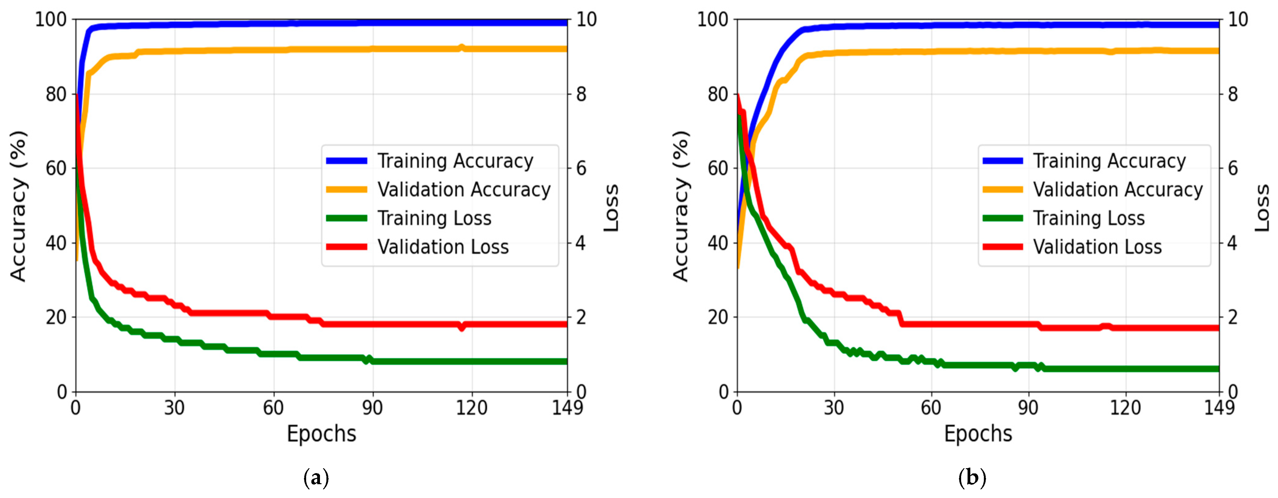
We used two open datasets: the BoniRob dataset [24] as Dataset A and the CWFID [25] as Dataset B. The BoniRob dataset contains 496 images with pixel-level annotated masks, while the CWFID contains 60 images with the same pixel-level annotated masks. Both dataset images were captured by an autonomous robot in the field at a resolution of 1296 × 966 pixels. For small training datasets, we use only a single image, and augmentation produces an additional image. We utilized two images (one augmented and one small training data) for training. During training, we reduced the image size to 512 × 512 pixels. We experimented on a Windows-based desktop system with an Intel Core i5-2320 CPU @ 3.00 GHz processor [54], a GPU of NVIDIA GeForce GTX 1070 [55] with 8 gigabytes of memory, and 16 gigabytes of RAM. For development, we utilized the PyTorch [56] platform in Python version 3.8 [57].

4.2. Training Setup

For Experiment 1, Dataset A was first used for training with 70% of the data. Dataset B, transformed using the proposed method, was subsequently divided into two equal portions: one serving as testing data and the other as small training data. A single image of the small training data was then augmented and used for training, whereas the testing data remained unchanged. In Experiment 2, 70% of the data in Dataset B were used for training. Next, the data were preprocessed, and Dataset A was subsequently divided into two equal portions: one serving as testing data and the other as small training data. We augmented a single image of the small training data and further utilized it for training, while the test data remained unchanged. During training, the images underwent resizing to a resolution of 512 × 512 pixels, and the network was trained using a batch size of two for 150 epochs. We employed an Adam optimizer [58] with an initial learning rate (LR) of 1 × 10⁻⁵ and utilized a cosine annealing strategy [59] to steadily reduce the LR during training. The training loss was calculated using dice loss [60]. We trained the proposed framework using the U-Net, modified U-Net, and CED-Net architectures. Figure 9 depicts the loss and training graphs for the BoniRob dataset and the CWFID using U-Net. Furthermore, the convergence of the loss and accuracy curves of the validation and training data demonstrates that the network is adequately trained and avoids overfitting.

Figure 9. Accuracy and loss graphs of training and validation data from (a) BoniRob dataset and (b) CWFID.

4.3. Evaluation Metrics

The experiment aimed to assess the semantic segmentation performance across three classes (background, crop, and weed) using evaluation metrics including precision, the mean intersection of union (mIoU), recall, and weighted harmonic mean of precision and recall (F1-score), as outlined in Equations (23)–(27). These values were used to calculate the overall segmentation performance of the proposed framework. The number of classes was set to three. The evaluation metrics used to determine the accuracy of segmentation included true negative (TN), true positive (TP), false negative (FN), and false positive (FP) values. When the true and false labels match the prediction, the scenario is usually referred to as a TN or TP. FP and FN are terms used to describe scenarios in which an incorrect label is mistakenly anticipated as true and a valid label is mistakenly anticipated as a false label.

$$\mathrm{I}\mathrm{o}\mathrm{U}=\frac{\mathrm{T}\mathrm{P}}{\mathrm{T}\mathrm{P}+\mathrm{F}\mathrm{N}+\mathrm{F}\mathrm{P}},$$

(23)

$$\mathrm{m}\mathrm{I}\mathrm{o}\mathrm{U}\mathrm{ }=\mathrm{ }\frac{{\sum }_{\mathrm{j}=1}^{\mathrm{C}\mathrm{l}\mathrm{s}}\mathrm{ }\mathrm{I}\mathrm{O}{\mathrm{U}}_{\mathrm{j}}}{\mathrm{C}\mathrm{l}\mathrm{s}},$$

(24)

$$\mathrm{R}\mathrm{e}\mathrm{c}\mathrm{a}\mathrm{l}\mathrm{l}=\frac{\mathrm{T}\mathrm{P}}{\mathrm{T}\mathrm{P}+\mathrm{F}\mathrm{N}},$$

(25)

$$\mathrm{P}\mathrm{r}\mathrm{e}\mathrm{c}\mathrm{i}\mathrm{s}\mathrm{i}\mathrm{o}\mathrm{n}=\frac{\mathrm{T}\mathrm{P}}{\mathrm{T}\mathrm{P}+\mathrm{F}\mathrm{P}},$$

(26)

$$\mathrm{F}1-\mathrm{score}=\frac{2\times \mathrm{P}\mathrm{r}\mathrm{e}\mathrm{c}\mathrm{i}\mathrm{s}\mathrm{i}\mathrm{o}\mathrm{n}\times \mathrm{R}\mathrm{e}\mathrm{c}\mathrm{a}\mathrm{l}\mathrm{l}}{\mathrm{P}\mathrm{r}\mathrm{e}\mathrm{c}\mathrm{i}\mathrm{s}\mathrm{i}\mathrm{o}\mathrm{n}+\mathrm{R}\mathrm{e}\mathrm{c}\mathrm{a}\mathrm{l}\mathrm{l}}$$

(27)

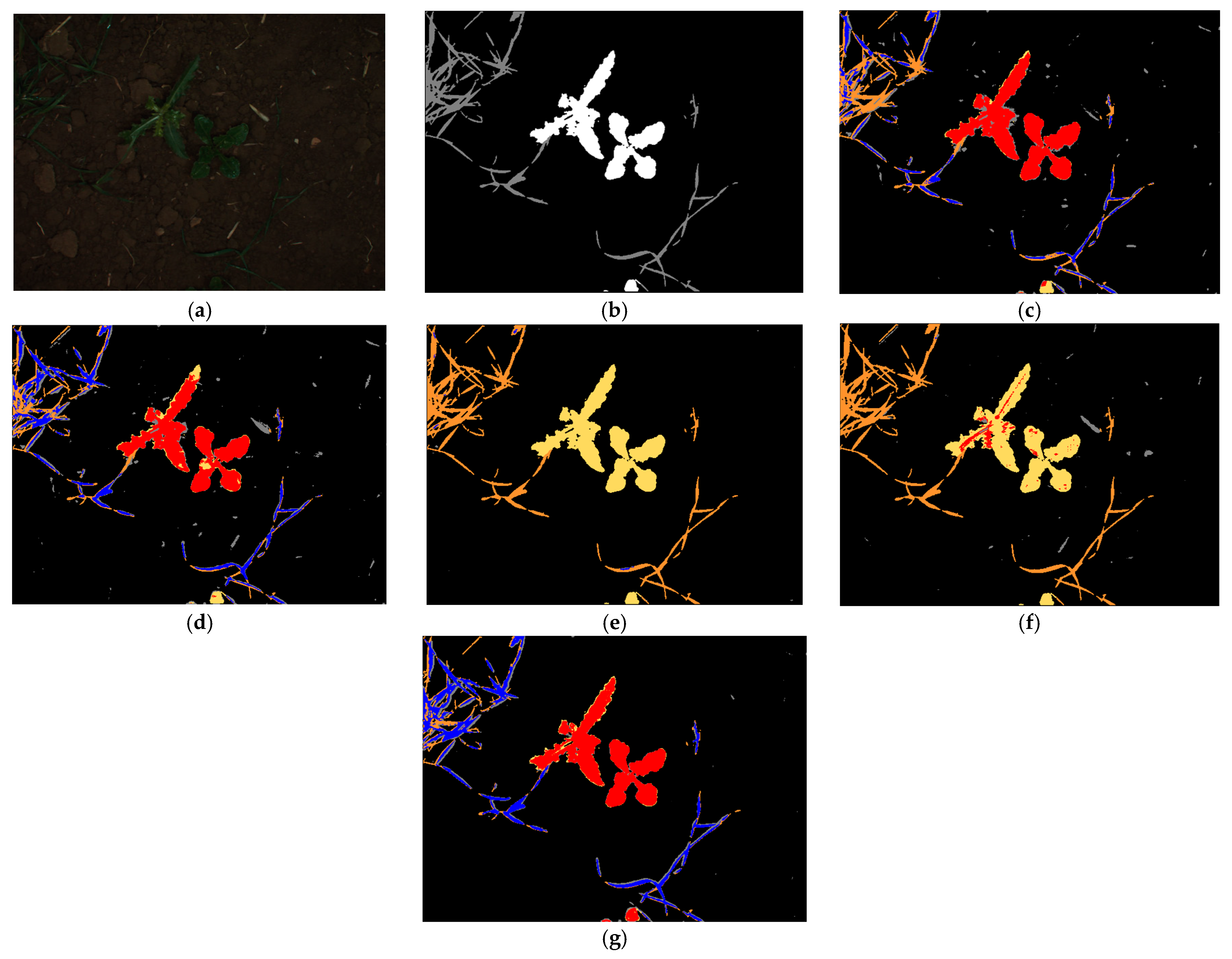
4.4. Testing for the Proposed Framework

Below is the explanation of the experimental results of the proposed framework for semantic segmentation in Experiments 1 and 2.

4.4.1. Testing with CWFID after Training with BoniRob Dataset

Ablation Study

In the ablation studies, we conducted several experiments across various scenarios, encompassing six different cases outlined in Table 2.

Table 2. Representation of various cases.

Cases	RH Transformation	Using One Training Data	Data Augmentation
Case I
Case II	✔
Case III		✔
Case IV	✔	✔
Case V		✔	✔
Case VI	✔	✔	✔

We repeated these six cases in Experiments 1 and 2. Table 3, Table 4 and Table 5 present the results of Experiment 1 for semantic segmentation using segmentation networks including U-Net, modified U-Net, and CED-Net. Across all experiments, Case I showed the lowest performance, and Case VI (the proposed method) showed the highest performance. This confirms that the proposed schemes of using RH transformation, one training dataset, and DA can enhance segmentation accuracy in all the segmentation models. In addition, the semantic segmentation performance of Case VI and U-Net is the best.

Table 3. Comparisons of different cases using U-Net (Experiment 1) (Cr means crop, Wd means weed, Bg means background, Re means recall, and Pre means precision).

Model	Cases	mIoU	IoU (Cr)	IoU (Wd)	IoU (Bg)	Re	Pre	F1-Score
U-Net	Case I	0.384	0.001	0.195	0.384	0.643	0.403	0.495
	Case II	0.423	0.098	0.206	0.965	0.638	0.567	0.594
	Case III	0.493	0.322	0.175	0.982	0.621	0.605	0.611
	Case IV	0.589	0.472	0.309	0.985	0.732	0.721	0.724
	Case V	0.499	0.294	0.221	0.982	0.652	0.627	0.639
	Case VI (proposed)	0.620	0.524	0.349	0.986	0.762	0.749	0.752

Table 4. Comparisons of different cases using modified U-Net (Experiment 1) (Cr means crop, Wd means weed, Bg means background, Re means recall, and Pre means precision).

Model	Cases	mIoU	IoU (Cr)	IoU (Wd)	IoU (Bg)	Re	Pre	F1-Score
Modified U-Net	Case I	0.380	0.006	0.195	0.941	0.645	0.406	0.497
	Case II	0.427	0.104	0.209	0.968	0.657	0.563	0.601
	Case III	0.483	0.244	0.221	0.983	0.646	0.608	0.625
	Case IV	0.523	0.368	0.217	0.984	0.664	0.635	0.648
	Case V	0.471	0.195	0.234	0.983	0.656	0.615	0.634
	Case VI (proposed)	0.539	0.382	0.251	0.984	0.686	0.665	0.674

Table 5. Comparisons of different cases using CED-Net (Experiment 1) (Cr means crop, Wd means weed, Bg means background, Re means recall, and Pre means precision).

Model	Cases	mIoU	IoU (Cr)	IoU (Wd)	IoU (Bg)	Re	Pre	F1-Score
CED-Net	Case I	0.387	0.009	0.196	0.956	0.634	0.441	0.518
	Case II	0.396	0.018	0.209	0.962	0.616	0.465	0.528
	Case III	0.461	0.234	0.175	0.974	0.603	0.559	0.579
	Case IV	0.516	0.409	0.168	0.971	0.640	0.592	0.614
	Case V	0.466	0.235	0.188	0.974	0.617	0.564	0.589
	Case VI (proposed)	0.521	0.472	0.120	0.972	0.637	0.613	0.624

An ablation study is presented in Table 6 to show the significance of the selection of the mean and std values for the RH transformation in the proposed framework. In this ablation study, we used the same training data as in the ablation study experiments with U-Net of Case VI (Table 3) and performed testing to validate the performance difference between the RH transformation and RH transformation with additional adjustment values that deviate from the selected values. We set the RH transformation with additional adjustment values to make the distribution of channels akin to that of the reference image in the histograms, as shown in Figure 3 and explained in Section 3.2.2. The performance results (F1-score) with additional adjustment values are 13.1% lower than those with the RH transformation without additional adjustments, as listed in Table 6. Although the RH transformation with additional adjustments makes the relative channel distributions similar between the target and reference images, as shown in Figure 3, it results in a greater decrease in the absolute numbers of red and green channels. Additionally, the mean of all channels decreases and moves toward zero, which reduces contrast and illumination, as shown in Figure 3. Moreover, the variance also increases, and all factors collectively cause the performance degradation of the RH transformation with additional adjustments.

Table 6. Comparison of results between RH transformation and RH transformation with additional adjustments (Cr means crop, Wd means weed, Bg means background, Re means recall, and Pre means precision).

Experiment	mIoU	IoU (Cr)	IoU (Wd)	IoU (Bg)	Re	Pre	F1-Score
RH transformation	0.620	0.524	0.349	0.986	0.762	0.749	0.752
RH transformation with additional adjustments	0.468	0.199	0.229	0.975	0.631	0.615	0.621

Visual examples of the semantic segmentation results using U-Net, modified U-Net, and CED-Net are illustrated in Figure 10. In this illustration, red pixels represent the TP of crops, black pixels represent the TP of the background, and blue pixels signify the TP of the weed. Yellow pixels represent errors where crops were mistakenly identified as background or weeds, while orange pixels represent errors where weeds were mistakenly identified as background or crops. Gray pixels indicate errors where the background was mistakenly identified as weeds or crops. As depicted in the figure, the utilization of U-Net in the proposed framework demonstrates superior semantic segmentation accuracy.

Figure 10. Visual comparisons of various semantic segmentation outputs with proposed framework (Experiment 1): (a) original image; (b) RH-transformed image; (c) ground-truth mask; semantic segmentation results with (d) CED-Net; (e) modified U-Net, and (f) U-Net.

Performance Comparisons of the Proposed Framework with SOTA Transformations

We analyzed the SOTA transformations with those of the proposed method employing U-Net, modified U-Net, and CED-Net, as outlined in Table 7. Our findings confirm that the proposed framework yields the highest outcomes across all segmentation networks. Additionally, Table 7 reveals that U-Net within the proposed framework attains the highest segmentation performance for both crops and weeds.

Table 7. Performance comparisons of proposed method and SOTA transformations (Cr means crop, Wd means weed, Bg means background, Re means recall, and Pre means precision).

Segmentation Model	Transformation	mIoU	IoU (Cr)	IoU (Wd)	IoU (Bg)	Re	Pre	F1-Score
U-Net	Xiao et al. [61]	0.496	0.257	0.274	0.958	0.717	0.583	0.640
	Pitie et al. [62]	0.548	0.378	0.312	0.953	0.776	0.601	0.675
	Gatys et al. [63]	0.457	0.313	0.101	0.958	0.558	0.575	0.563
	Nguyen et al. [64]	0.487	0.486	0.010	0.964	0.563	0.580	0.569
	Proposed	0.620	0.524	0.349	0.986	0.762	0.749	0.752
Modified U-Net	Xiao et al. [61]	0.387	0.066	0.161	0.934	0.651	0.494	0.558
	Pitie et al. [62]	0.462	0.200	0.221	0.966	0.716	0.569	0.630
	Gatys et al. [63]	0.396	0.157	0.083	0.948	0.452	0.544	0.490
	Nguyen et al. [64]	0.427	0.136	0.185	0.959	0.518	0.580	0.545
	Proposed	0.539	0.382	0.251	0.984	0.686	0.665	0.674
CED-Net	Xiao et al. [61]	0.390	0.036	0.204	0.928	0.618	0.447	0.518
	Pitie et al. [62]	0.394	0.109	0.180	0.894	0.673	0.472	0.553
	Gatys et al. [63]	0.360	0.000	0.143	0.938	0.605	0.378	0.465
	Nguyen et al. [64]	0.310	0.000	0.065	0.865	0.479	0.349	0.402
	Proposed	0.521	0.472	0.120	0.972	0.637	0.613	0.624

Visual examples of SOTA transformations and the proposed method using U-Net are shown in Figure 11. In this illustration, red pixels represent the TP of crops, black pixels represent the TP of the background, and blue pixels signify the TP of the weed. Yellow pixels represent errors where crops were mistakenly identified as background or weeds, while orange pixels represent errors where weeds were mistakenly identified as background or crops. Gray pixels indicate errors where the background was mistakenly identified as weeds or crops. As depicted in the figure, the proposed framework demonstrates the highest semantic segmentation accuracy.

Figure 11. Visual comparisons of various SOTA transformations with the proposed framework using U-Net (Experiment 1): (a) original image; (b) ground-truth mask; semantic segmentation results with (c) Xiao et al.; (d) Pitie et al.; (e) Gatys et al.; (f) Nguyen et al.; and (g) proposed method.

4.4.2. Testing with BoniRob Dataset after Training with CWFID

Ablation Study

For the ablation studies, six cases were considered in Experiment 2, as described in the Ablation Study of Section 4.4.1. Table 8, Table 9 and Table 10 present the results of Experiment 2 for semantic segmentation using segmentation networks. From these tables, we can observe that the accuracy is lower for Cases I, III, and IV without RH transformation for the test data, but the performance improved when we used RH transformation in Cases II, IV, and VI. In Case VI, the proposed framework shows the highest accuracy among all segmentation networks and the best accuracy with U-Net.

Table 8. Comparison of different cases using U-Net (Experiment 2) (Cr means crop, Wd means weed, Bg means background, Re means recall, and Pre means precision).

Model	Cases	mIoU	IoU (Cr)	IoU (Wd)	IoU (Bg)	Re	Pre	F1-Score
U-Net	Case I	0.316	0.000	0.000	0.948	0.333	0.329	0.330
	Case II	0.570	0.230	0.508	0.971	0.704	0.679	0.688
	Case III	0.494	0.227	0.286	0.969	0.630	0.673	0.649
	Case IV	0.621	0.272	0.621	0.969	0.779	0.689	0.730
	Case V	0.507	0.232	0.322	0.968	0.645	0.679	0.659
	Case VI (proposed)	0.637	0.292	0.647	0.971	0.787	0.708	0.743

Table 9. Comparison of different cases using modified U-Net (Experiment 2) (Cr means crop, Wd means weed, Bg means background, Re means recall, and Pre means precision).

Model	Cases	mIoU	IoU (Cr)	IoU (Wd)	IoU (Bg)	Re	Pre	F1-Score
Modified U-Net	Case I	0.316	0.000	0.000	0.948	0.333	0.316	0.324
	Case II	0.529	0.235	0.383	0.970	0.682	0.665	0.668
	Case III	0.448	0.212	0.163	0.968	0.588	0.596	0.589
	Case IV	0.605	0.266	0.593	0.955	0.833	0.651	0.728
	Case V	0.477	0.232	0.232	0.966	0.633	0.611	0.619
	Case VI (proposed)	0.622	0.294	0.610	0.962	0.837	0.667	0.739

Table 10. Comparison of different cases using CED-Net (Experiment 2) (Cr means crop, Wd means weed, Bg means background, Re means recall, and Pre means precision).

Model	Cases	mIoU	IoU (Cr)	IoU (Wd)	IoU (Bg)	Re	Pre	F1-Score
CED-Net	Case I	0.315	0.000	0.000	0.946	0.332	0.318	0.322
	Case II	0.487	0.176	0.336	0.951	0.699	0.564	0.621
	Case III	0.488	0.013	0.572	0.879	0.624	0.537	0.575
	Case IV	0.552	0.218	0.504	0.935	0.838	0.592	0.691
	Case V	0.485	0.0143	0.581	0.860	0.623	0.539	0.576
	Case VI (proposed)	0.570	0.244	0.519	0.946	0.836	0.611	0.703

We can see the visual examples of semantic segmentation outputs using U-Net, modified U-Net, and CED-Net in Figure 12. In this illustration, red pixels represent the TP of crops, black pixels represent the TP of the background, and blue pixels signify the TP of the weed. Yellow pixels represent errors where crops were mistakenly identified as background or weeds, while orange pixels represent errors where weeds were mistakenly identified as background or crops. Gray pixels indicate errors where the background was mistakenly identified as weeds or crops. As depicted in the figure, the proposed framework with U-Net demonstrates the highest semantic segmentation accuracy.

Figure 12. Visual comparisons of various semantic segmentation outputs with proposed framework (Experiment 1): (a) original image; (b) RH-transformed image; (c) ground-truth mask; semantic segmentation results with (d) CED-Net; (e) modified U-Net, and (f) U-Net.

Performance Comparisons of the Proposed Framework with SOTA Transformations

In this subsection, we compared the SOTA transformations with those of the proposed framework using U-Net, modified U-Net, and CED-Net, as listed in Table 11. We verify that the proposed framework shows superior performance over all segmentation networks. Moreover, Table 11 highlights that U-Net, when utilized within the proposed framework, obtained the highest semantic segmentation accuracy for crops and weeds.

Table 11. Comparisons of the performance of the proposed method and SOTA transformations (Cr means crop, Wd means weed, Bg means background, Re means recall, and Pre means precision).

Model	Transformation	mIoU	IoU (Cr)	IoU (Wd)	IoU (Bg)	Re	Pre	F1-Score
U-Net	Xiao et al. [61]	0.530	0.505	0.124	0.962	0.696	0.589	0.635
	Pitie et al. [62]	0.543	0.475	0.193	0.959	0.729	0.605	0.657
	Gatys et al. [63]	0.316	0.000	0.000	0.948	0.333	0.381	0.352
	Nguyen et al. [64]	0.332	0.049	0.000	0.946	0.352	0.417	0.379
	Proposed	0.637	0.647	0.292	0.971	0.787	0.708	0.743
Modified U-Net	Xiao et al. [61]	0.526	0.521	0.145	0.911	0.787	0.573	0.661
	Pitie et al. [62]	0.516	0.522	0.141	0.886	0.817	0.567	0.667
	Gatys et al. [63]	0.316	0.000	0.000	0.948	0.333	0.320	0.326
	Nguyen et al. [64]	0.187	0.014	0.031	0.516	0.387	0.368	0.375
	Proposed	0.622	0.610	0.294	0.962	0.837	0.667	0.739
CED-Net	Xiao et al. [61]	0.423	0.339	0.067	0.862	0.709	0.475	0.566
	Pitie et al. [62]	0.466	0.442	0.107	0.850	0.807	0.524	0.632
	Gatys et al. [63]	0.318	0.005	0.018	0.932	0.338	0.340	0.339
	Nguyen et al. [64]	0.316	0.000	0.001	0.948	0.333	0.375	0.349
	Proposed	0.570	0.519	0.244	0.946	0.836	0.611	0.703

Visual examples of SOTA transformations and the proposed method using U-Net are illustrated in Figure 13. In this illustration, red pixels represent the TP of crops, black pixels represent the TP of the background, and blue pixels signify the TP of the weed. Yellow pixels represent errors where crops were mistakenly identified as background or weeds, while orange pixels represent errors where weeds were mistakenly identified as background or crops. Gray pixels indicate errors where the background was mistakenly identified as weeds or crops. As illustrated in the figure, the proposed framework demonstrates the highest semantic segmentation accuracy.

Figure 13. Visual comparisons of various SOTA transformations with proposed framework using U-Net (Experiment 1): (a) original image; (b) ground-truth mask; semantic segmentation results with (c) Xiao et al.; (d) Pitie et al.; (e) Gatys et al.; (f) Nguyen et al.; and (g) proposed method.

4.5. Fractal Dimension Estimation

The FD is used as a mathematical metric to characterize the complexity of geometric structures, particularly fractal shapes, which exhibit self-similarity across different scales. Fractal shapes possess similar patterns or structures across different scales, and the complexity of these shapes can be quantified using a numerical value of FD that generally ranges between one and two [65]. A higher FD value indicates greater complexity. A common method for computing the FD is the box-counting algorithm [66]. We refer to the box-counting algorithm [12] to compute the FD, which was implemented by the PyTorch [56] platform in Python version 3.8 [57]. Algorithm 2 provides the pseudo-code to measure the FD.

Algorithm 2: Pseudo-code for measuring FD

Input: image (path to the input image)

Output: Fractal dimension (FD) value

1:  Read the input image and further convert it into grayscale 2:   Set the maximum box-size with the power of 2 and ensure the dimensions      s = 2^(log(max(size(image))/log2)]     Add the padding if required to match the dimensions 3:   Compute the number of boxes N(s) till minimum pixels 4:   Reduce box size by 2 and recalculate N(s) iteratively     while s > 1 5:   Compute log(N(s)) and log(1/s) for each s 6:   Draw a fitted line to the points (log(N(s)) and log(1/s))

7:  FD value is the slope of the fitted line    Return Fractal Dimension Value

The algorithm enables the calculation of the FD for both precise and approximate self-affine patterns and has wide applications across various natural and manmade systems [13,67]. The formula employed to estimate the FD utilizing the box-counting algorithm [12] is as follows:

$$\mathrm{FD}={\lim }_{\mathrm{s}\text{→}0}\frac{\log \left(\mathrm{N}\right(\mathrm{s}\left)\right)}{\log (1/\mathrm{s})}$$

(28)

where $\mathrm{N}\left(\mathrm{s}\right)$ represents the sum of boxes of size $\mathrm{s}$, and FD signifies the fractal dimension defining the curve being analyzed. We employed a box-counting technique to calculate the approximate FD of various shapes. The method was evaluated using two datasets, BoniRob and CWFID. The experimental results are presented in Table 12, demonstrating the FD values and distribution of crops and weeds across different sections of the field. The 1st–3rd row FD values in Table 12 were computed from the 1st~3rd row images in Figure 14. In addition, the 4th~6th row FD values in Table 12 were computed from the 4th~6th row images in Figure 15. Higher FD values for crops and weeds represent the high complexities of crops and weeds, suggesting that farming experts or robots should pay more attention to discriminating between crops and weeds. This estimation technique can also automate farming systems by targeting and eliminating weeds through precise spraying in areas with high weed complexity, ultimately increasing the crop yield.

Table 12. FD values of images from CWFID and BoniRob dataset. The 1st~3rd row FD values are computed from the 1st~3rd row images of Figure 14. The 4th~6th row FD values are computed from the 4th~6th row images of Figure 15.

Dataset	Weed FD	Crop FD
CWFID	1.61	1.26
	0.76	1.43
	1.53	1.21
BoniRob dataset	1.27	0.91
	1.32	1.31
	0.97	1.54

Figure 14. Visual representation of crops and weeds with samples from the CWFID for estimating FD values: (a) whole segmentation results; (b) weed segmentation result; and (c) crop segmentation result.

Figure 15. Visual representation of crops and weeds with samples from the BoniRob dataset for estimating FD values: (a) whole segmentation results; (b) weed segmentation result; and (c) crop segmentation result.

4.6. Comparisons of Processing Time

In this section, we compare the average processing times per image obtained using the proposed method with those obtained using the SOTA method. The unit ms denotes milliseconds. Table 13 illustrates that the method by Xiao et al. [61] exhibits the highest processing time, whereas the method by Nguyen et al. [64] demonstrates the lowest processing time. Interestingly, our proposed framework falls at the second lowest in processing time (as indicated in Table 13). Although the proposed framework has a higher processing time than Nguyen et al. [64], our goal is to achieve high accuracies of crop and weed segmentation. The proposed framework with U-Net yields better results than the SOTA methods, as evidenced in Table 7 and Table 11 and Figure 11 and Figure 13.

Table 13. Comparisons of average processing time by proposed and SOTA methods (unit: ms).

Methods	Processing Time
Xiao et al. [61]	1270
Pitie et al. [62]	2920
Gatys et al. [63]	2210
Nguyen et al. [64]	1030
Proposed	1080

5. Discussion

We performed statistical analysis using the Student’s t-test [68] and calculated the Cohen’s d-value [69]. For this purpose, we calculated the mean and std of the mIoU using our method with U-Net, as shown in Table 7 and Table 11, respectively. Additionally, we calculated the mean and std of the mIoU using the second-best method (Pitie et al. [62]) with U-Net, as presented in Table 7 and Table 11. The measured p-value is 0.041, showing a confidence level of 95% with a significant difference, as depicted in Figure 16, and Cohen’s d-value is 0.936, representing a large effect size. This confirms that the proposed framework statistically surpasses the second-best method and achieves higher segmentation accuracy.

Figure 16. T-test results.

We also analyzed the semantic segmentation performance using the proposed method with U-Net based on gradient-weighted class activation mapping (Grad-CAM) [70], as depicted in Figure 17. Grad-CAM typically depicts important features as reddish and yellowish colors, whereas unimportant features are shown in bluish colors as explainable artificial intelligence. Figure 17 shows the Grad-CAM image, obtained after the fourth convolution layer of U-Net, illustrating the accurate extraction of crucial features for crop and weed segmentation, confirming that our method can generate correct images in heterogeneous datasets for the accurate segmentation of crops and weeds.

Figure 17. Sample images of the CWFID with Grad-CAM visualization after the 4th convolution layer. (a) Input image, (b) ground-truth mask (gray, white, and black pixels mean weeds, crops, and background, respectively), (c) Grad-CAM of class 1 (weed), (d) Grad-CAM of class 2 (crop), and (e) segmented results.

Figure 18 shows examples of incorrect segmentation using the proposed method with U-Net. In this illustration, red pixels represent the TP of crops, black pixels represent the TP of the background, and blue pixels signify the TP of the weed. Yellow pixels represent errors where crops were mistakenly identified as background or weeds, while orange pixels represent errors where weeds were mistakenly identified as background or crops. Gray pixels indicate errors where the background was mistakenly identified as weeds or crops. The reason for the incorrect segmentation is that crops and weeds have similar shapes and colors, making them hard to distinguish, especially in cases where objects possess thin regions.

Figure 18. Samples of incorrect segmentation generated by proposed method with U-Net: (a) original image; (b) RH-transformed image; (c) ground-truth mask; and (d) semantic segmentation results.

As automation in agriculture is a subject of intensive research, it has led to many reformations in agriculture, such as saving time, reducing manpower, increasing yields through proper monitoring systems, and precise crop and weed detection. In agricultural precision for heterogeneous data, our proposed framework exhibits great performance, segregating crops and weeds accurately, which can increase yield and drive the transition to modern agriculture.

6. Conclusions

In this study, we introduce an approach for segmenting crops and weeds and estimating the FD using small amounts of training data in a heterogeneous data environment. This is the first study on the segmentation of crops and weeds within a heterogeneous environmental setup utilizing one training data sample. We rigorously investigated the factors that cause performance degradation in heterogeneous datasets, including variations in illumination and contrast. To solve this challenge, we proposed a framework that leverages mean and standard deviation adjustments using the RH transformation. Furthermore, we improved the performance using a small amount of training data. This additional small amount of training data significantly improves the segmentation performance with reduced computational power and training time. In addition, we introduced an FD estimation approach in our system, which was smoothly combined as an end-to-end task to furnish crucial insights into the distributional characteristics of crops and weeds. Through experiments using two open databases, we proved that our approach outperforms the SOTA method. Additionally, we confirmed that our approach showed statistically superior results than the second-best method in terms of the t-test and Cohen’s d-value. Furthermore, using Grad-CAM images, we validated the capability of the proposed method to extract essential features necessary for the accurate segmentation of crops and weeds. Nonetheless, instances of inaccurate segmentation were observed in scenarios where crops and weeds exhibit comparable colors, shapes, and thin regions, as depicted in Figure 18.

To address this issue, we would research the generative adversarial network-based transformation method for the correct segmentation of small-sized and thin crops and weeds having similar colors and shapes in heterogeneous data environments. Moreover, we applied our method to other tasks, such as box-based detection or classification in heterogeneous data environments. In addition, we would check the possibility of applying our method to other application areas including crack detection for building monitoring, medical image detection, and underwater computer vision.

References

1. Jiang, Y.; Li, C. Convolutional Neural Networks for Image-Based High-Throughput Plant Phenotyping: A Review. Plant Phenomics 2020, 2020, 4152816. [Google Scholar] [CrossRef] [PubMed]
2. Fathipoor, H.; Arefi, H.; Shah-Hosseini, R.; Moghadam, H. Corn Forage Yield Prediction Using Unmanned Aerial Vehicle Images at Mid-Season Growth Stage. J. Appl. Remote Sens 2019, 13, 034503. [Google Scholar] [CrossRef]
3. Yang, Q.; Wang, Y.; Liu, L.; Zhang, X. Adaptive Fractional-Order Multi-Scale Optimization TV-L1 Optical Flow Algorithm. Fractal Fract. 2024, 8, 8040179. [Google Scholar] [CrossRef]
4. Huang, T.; Wang, X.; Xie, D.; Wang, C.; Liu, X. Depth Image Enhancement Algorithm Based on Fractional Differentiation. Fractal Fract. 2023, 7, 7050394. [Google Scholar] [CrossRef]
5. Bai, X.; Zhang, D.; Shi, S.; Yao, W.; Guo, Z.; Sun, J. A Fractional-Order Telegraph Diffusion Model for Restoring Texture Images with Multiplicative Noise. Fractal Fract. 2023, 7, 7010064. [Google Scholar] [CrossRef]
6. AlSheikh, M.H.; Al-Saidi, N.M.G.; Ibrahim, R.W. Dental X-ray Identification System Based on Association Rules Extracted by k-Symbol Fractional Haar Functions. Fractal Fract. 2022, 6, 6110669. [Google Scholar] [CrossRef]
7. Zhang, Y.; Yang, L.; Li, Y. A Novel Adaptive Fractional Differential Active Contour Image Segmentation Method. Fractal Fract. 2022, 6, 6100579. [Google Scholar] [CrossRef]
8. Zhang, Y.; Liu, T.; Yang, F.; Yang, Q. A Study of Adaptive Fractional-Order Total Variational Medical Image Denoising. Fractal Fract. 2022, 6, 6090508. [Google Scholar] [CrossRef]
9. Jiao, Q.; Liu, M.; Ning, B.; Zhao, F.; Dong, L.; Kong, L.; Hui, M.; Zhao, Y. Image Dehazing Based on Local and Non-Local Features. Fractal Fract. 2022, 6, 6050262. [Google Scholar] [CrossRef]
10. Zhang, X.; Dai, L. Image Enhancement Based on Rough Set and Fractional Order Differentiator. Fractal Fract. 2022, 6, 6040214. [Google Scholar] [CrossRef]
11. Zhang, X.; Liu, R.; Ren, J.; Gui, Q. Adaptive Fractional Image Enhancement Algorithm Based on Rough Set and Particle Swarm Optimization. Fractal Fract. 2022, 6, 6020100. [Google Scholar] [CrossRef]
12. Cheng, J.; Chen, Q.; Huang, X. An Algorithm for Crack Detection, Segmentation, and Fractal Dimension Estimation in Low-Light Environments by Fusing FFT and Convolutional Neural Network. Fractal Fract. 2023, 7, 7110820. [Google Scholar] [CrossRef]
13. An, Q.; Chen, X.; Wang, H.; Yang, H.; Yang, Y.; Huang, W.; Wang, L. Segmentation of Concrete Cracks by Using Fractal Dimension and UHK-Net. Fractal Fract. 2022, 6, 6020095. [Google Scholar] [CrossRef]
14. Sultan, H.; Owais, M.; Park, C.; Mahmood, T.; Haider, A.; Park, K.R. Artificial Intelligence-Based Recognition of Different Types of Shoulder Implants in X-Ray Scans Based on Dense Residual Ensemble-Network for Personalized Medicine. J. Pers. Med. 2021, 11, 11060482. [Google Scholar] [CrossRef] [PubMed]
15. Arsalan, M.; Haider, A.; Hong, J.S.; Kim, J.S.; Park, K.R. Deep Learning-Based Detection of Human Blastocyst Compartments with Fractal Dimension Estimation. Fractal Fract. 2024, 8, 8050267. [Google Scholar] [CrossRef]
16. González-Sabbagh, S.P.; Robles-Kelly, A. A Survey on Underwater Computer Vision. ACM Comput. Surv. 2023, 55, 1–39. [Google Scholar] [CrossRef]
17. Madokoro, H.; Takahashi, K.; Yamamoto, S.; Nix, S.; Chiyonobu, S.; Saruta, K.; Saito, T.K.; Nishimura, Y.; Sato, K. Semantic Segmentation of Agricultural Images Based on Style Transfer Using Conditional and Unconditional Generative Adversarial Networks. Appl. Sci. 2022, 12, 12157785. [Google Scholar] [CrossRef]
18. Kim, Y.; Park, K.R. MTS-CNN: MTS-CNN: Multi-Task Semantic Segmentation-Convolutional Neural Network for Detecting Crops and Weeds. Comput. Electron. Agric. 2022, 199, 107146. [Google Scholar] [CrossRef]
19. Wang, R.; Jiao, L.; Xie, C.; Chen, P.; Du, J.; Li, R. S-RPN: Sampling-Balanced Region Proposal Network for Small Crop Pest Detection. Comput. Electron. Agric. 2021, 187, 106290. [Google Scholar] [CrossRef]
20. Huang, S.; Wu, S.; Sun, C.; Ma, X.; Jiang, Y.; Qi, L. Deep Localization Model for Intra-Row Crop Detection in Paddy Field. Comput. Electron. Agric. 2020, 169, 105203. [Google Scholar] [CrossRef]
21. Kang, J.; Liu, L.; Zhang, F.; Shen, C.; Wang, N.; Shao, L. Semantic Segmentation Model of Cotton Roots In-Situ Image Based on Attention Mechanism. Comput. Electron. Agric. 2021, 189, 106370. [Google Scholar] [CrossRef]
22. Le Louëdec, J.; Cielniak, G. 3D Shape Sensing and Deep Learning-Based Segmentation of Strawberries. Comput. Electron. Agric. 2021, 190, 106374. [Google Scholar] [CrossRef]
23. Brilhador, A.; Gutoski, M.; Hattori, L.T.; de Souza Inácio, A.; Lazzaretti, A.E.; Lopes, H.S. Classification of Weeds and Crops at the Pixel-Level Using Convolutional Neural Networks and Data Augmentation. In Proceedings of the IEEE Latin American Conference on Computational Intelligence, Guayaquil, Ecuador, 11–15 November 2019; pp. 1–6. [Google Scholar] [CrossRef]
24. Chebrolu, N.; Lottes, P.; Schaefer, A.; Winterhalter, W.; Burgard, W.; Stachniss, C. Agricultural Robot Dataset for Plant Classification, Localization and Mapping on Sugar Beet Fields. Int. J. Robot. Res. 2017, 36, 1045–1052. [Google Scholar] [CrossRef]
25. Haug, S.; Ostermann, J. A Crop/Weed Field Image Dataset for the Evaluation of Computer Vision Based Precision Agriculture Tasks. In Proceedings of the Computer Vision—ECCV 2014 Workshops, Zurich, Switzerland, 6–7 and 12 September 2014; pp. 105–116. [Google Scholar] [CrossRef]
26. Nguyen, D.T.; Nam, S.H.; Batchuluun, G.; Owais, M.; Park, K.R. An Ensemble Classification Method for Brain Tumor Images Using Small Training Data. Mathematics 2022, 10, 10234566. [Google Scholar] [CrossRef]
27. Abdalla, A.; Cen, H.; Wan, L.; Rashid, R.; Weng, H.; Zhou, W.; He, Y. Fine-Tuning Convolutional Neural Network with Transfer Learning for Semantic Segmentation of Ground-Level Oilseed Rape Images in a Field with High Weed Pressure. Comput. Electron. Agric. 2019, 167, 105091. [Google Scholar] [CrossRef]
28. Crops and Weeds Segmentation Method in Heterogeneous Environment. Available online: https://github.com/iamrehanch/crops_and_weeds_semantic_segmentation (accessed on 9 March 2023).
29. Haug, S.; Michaels, A.; Biber, P.; Ostermann, J. Plant Classification System for Crop/Weed Discrimination without Segmentation. In Proceedings of the IEEE Winter Conference on Applications of Computer Vision, Steamboat Springs, CO, USA, 24–26 March 2014; pp. 1142–1149. [Google Scholar] [CrossRef]
30. Lottes, P.; Hörferlin, M.; Sander, S.; Stachniss, C. Effective Vision-Based Classification for Separating Sugar Beets and Weeds for Precision Farming: Effective Vision-Based Classification. J. Field Robot. 2017, 34, 1160–1178. [Google Scholar] [CrossRef]
31. Lottes, P.; Khanna, R.; Pfeifer, J.; Siegwart, R.; Stachniss, C. UAV-Based Crop and Weed Classification for Smart Farming. In Proceedings of the IEEE International Conference on Robotics and Automation, Singapore, Singapore, 29 May–3 June 2017; pp. 3024–3031. [Google Scholar] [CrossRef]
32. Yang, B.; Xu, Y. Applications of Deep-Learning Approaches in Horticultural Research: A Review. Hortic. Res. 2021, 8, 123. [Google Scholar] [CrossRef]
33. Chen, L.C.; Papandreou, G.; Schroff, F.; Adam, H. Rethinking Atrous Convolution for Semantic Image Segmentation. arXiv 2015, arXiv:1706.05587v3. [Google Scholar]
34. Long, J.; Shelhamer, E.; Darrell, T. Fully Convolutional Networks for Semantic Segmentation. In Proceedings of the IEEE Conference on Computer Vision and Pattern Recognition, Boston, MA, USA, 7–12 June 2015; pp. 3431–3440. [Google Scholar] [CrossRef]
35. Ronneberger, O.; Fischer, P.; Brox, T. U-Net: Convolutional Networks for Biomedical Image Segmentation. In Proceedings of the Medical Image Computing and Computer-Assisted Intervention, Munich, Germany, 5–9 October 2015; pp. 234–241. [Google Scholar] [CrossRef]
36. Badrinarayanan, V.; Kendall, A.; Cipolla, R. SegNet: A Deep Convolutional Encoder-Decoder Architecture for Image Segmentation. IEEE Trans. Pattern Anal. Mach. Intell. 2017, 39, 2481–2495. [Google Scholar] [CrossRef]
37. Zou, K.; Chen, X.; Wang, Y.; Zhang, C.; Zhang, F. A Modified U-Net with a Specific Data Argumentation Method for Semantic Segmentation of Weed Images in the Field. Comput. Electron. Agric. 2021, 187, 106242. [Google Scholar] [CrossRef]
38. Milioto, A.; Lottes, P.; Stachniss, C. Real-Time Semantic Segmentation of Crop and Weed for Precision Agriculture Robots Leveraging Background Knowledge in CNNs. In Proceedings of the IEEE International Conference on Robotics and Automation, Brisbane, Australia, 21–25 May 2018; pp. 2235–2299. [Google Scholar] [CrossRef]
39. Paszke, A.; Chaurasia, A.; Kim, S.; Culurciello, E. ENet: A Deep Neural Network Architecture for Real-Time Semantic Segmentation. arXiv 2016, arXiv:1606.02147v1. [Google Scholar]
40. Fathipoor, H.; Shah-Hosseini, R.; Arefi, H. Crop and Weed Segmentation on Ground_Based Images using Deep Convolutional Neural Network. In Proceedings of the ISPRS Annals of the Photogrammetry Remote Sensing and Spatial Information Sciences, Tehran, Iran, 13 January 2023; pp. 195–200. [Google Scholar] [CrossRef]
41. Zhou, Z.; Siddiquee, M.M.R.; Tajbakhsh, N.; Liang, J. UNet++: A Nested U-Net Architecture for Medical Image Segmentation. In Proceedings of the Deep Learning in Medical Image Analysis and Multimodal Learning for Clinical Decision Support, Granada, Spain, 20 September 2018; pp. 3–11. [Google Scholar] [CrossRef]
42. Simonyan, K.; Zisserman, A. Very Deep Convolutional Networks for Large-Scale Image Recognition. arXiv 2014, arXiv:1409.1556v6. [Google Scholar]
43. Fawakherji, M.; Potena, C.; Bloisi, D.D.; Imperoli, M.; Pretto, A.; Nardi, D. UAV Image Based Crop and Weed Distribution Estimation on Embedded GPU Boards. In Proceedings of the Computer Analysis of Images and Patterns, Salerno, Italy, 6 September 2019; pp. 100–108. [Google Scholar] [CrossRef]
44. Chakraborty, R.; Zhen, X.; Vogt, N.; Bendlin, B.; Singh, V. Dilated Convolutional Neural Networks for Sequential Manifold-Valued Data. In Proceedings of the IEEE/CVF International Conference on Computer Vision, Seoul, South Korea, 27 October—2 November 2019; pp. 10620–10630. [Google Scholar] [CrossRef]
45. You, J.; Liu, W.; Lee, J. A DNN-Based Semantic Segmentation for Detecting Weed and Crop. Comput. Electron. Agric. 2020, 178, 10570. [Google Scholar] [CrossRef]
46. Wang, H.; Song, H.; Wu, H.; Zhang, Z.; Deng, S.; Feng, X.; Chen, Y. Multilayer Feature Fusion and Attention-Based Network for Crops and Weeds Segmentation. J. Plant Dis. Prot. 2022, 129, 1475–1489. [Google Scholar] [CrossRef]
47. Siddiqui, S.A.; Fatima, N.; Ahmad, A. Neural Network Based Smart Weed Detection System. In Proceedings of the International Conference on Communication, Control and Information Sciences, Idukki, India, 16–18 June 2021; pp. 1–5. [Google Scholar] [CrossRef]
48. Khan, A.; Ilyas, T.; Umraiz, M.; Mannan, Z.I.; Kim, H. CED-Net: Crops and Weeds Segmentation for Smart Farming Using a Small Cascaded Encoder-Decoder Architecture. Electronics 2020, 9, 9101602. [Google Scholar] [CrossRef]
49. Reinhard, E.; Adhikhmin, M.; Gooch, B.; Shirley, P. Color Transfer between Images. IEEE Comput. Graph. Appl. 2001, 21, 34–41. [Google Scholar] [CrossRef]
50. Ruderman, D.L.; Cronin, T.W.; Chiao, C.C. Statistics of Cone Responses to Natural Images: Implications for Visual Coding. J. Opt. Soc. Am. A-Opt. Image Sci. Vis. 1998, 15, 2036–2045. [Google Scholar] [CrossRef]
51. Mikołajczyk, A.; Grochowski, M. Data Augmentation for Improving Deep Learning in Image Classification Problem. In Proceedings of the International Interdisciplinary PhD Workshop, Świnouście, Poland, 9–12 May 2018; pp. 117–122. [Google Scholar] [CrossRef]
52. Agarap, A.F. Deep Learning Using Rectified Linear Units (ReLU). arXiv 2019, arXiv:1803.08375v2. [Google Scholar]
53. Clevert, D.A.; Unterthiner, T.; Hochreiter, S. Fast and Accurate Deep Network Learning by Exponential Linear Units (ELUs). arXiv 2015, arXiv:1511.07289v5. [Google Scholar]
54. Intel Core i5-2320. Available online: https://www.intel.com/content/www/us/en/products/sku/53446/intel-core-i52320-processor-6m-cache-up_to-3-30-ghz/specifications.html (accessed on 5 October 2023).
55. NVIDIA GeForce GTX 1070. Available online: https://www.nvidia.com/en-gb/geforce/10-series/ (accessed on 5 October 2023).
56. PyTorch. Available online: https://pytorch.org/ (accessed on 5 October 2023).
57. Python 3.8. Available online: https://www.python.org/downloads/release/python-380/ (accessed on 5 October 2023).
58. Kingma, D.P.; Ba, J. Adam: A Method for Stochastic Optimization. arXiv 2014, arXiv:1412.6980v9. [Google Scholar]
59. Loshchilov, I.; Hutter, F. SGDR: Stochastic Gradient Descent with Warm Restarts. arXiv 2016, arXiv:1608.03983v5. Available online: https://arxiv.org/abs/1608.03983 (accessed on 5 October 2023).
60. Sudre, C.H.; Li, W.; Vercauteren, T.; Ourselin, S.; Cardoso, M.J. Generalised Dice Overlap as a Deep Learning Loss Function for Highly Unbalanced Segmentations. In Proceedings of the International Conference on Communication, Control and Information Sciences, Québec City, Canada, 9 September 2017; pp. 240–248. [Google Scholar] [CrossRef]
61. Xiao, X.; Ma, L. Color Transfer in Correlated Color Space. In Proceedings of the ACM International Conference on Virtual Reality Continuum and Its Applications, Hong Kong, China, 14 June 2006; pp. 305–309. [Google Scholar] [CrossRef]
62. Pitié, F.; Kokaram, A.C.; Dahyot, R. Automated Colour Grading Using Colour Distribution Transfer. Comput. Vis. Image Underst. 2007, 107, 123–137. [Google Scholar] [CrossRef]
63. Gatys, L.A.; Ecker, A.S.; Bethge, M. Image Style Transfer Using Convolutional Neural Networks. In Proceedings of the IEEE Conference on Computer Vision and Pattern Recognition, Las Vegas, NV, USA, 23–27 June 2016; pp. 2414–2423. [Google Scholar] [CrossRef]
64. Nguyen, R.M.H.; Kim, S.J.; Brown, M.S. Illuminant Aware Gamut-Based Color Transfer. Comput. Graph. Forum 2014, 33, 319–328. [Google Scholar] [CrossRef]
65. Rezaie, A.; Mauron, A.J.; Beyer, K. Sensitivity Analysis of Fractal Dimensions of Crack Maps on Concrete and Masonry Walls. Autom.Constr. 2020, 117, 103258. [Google Scholar] [CrossRef]
66. Wu, J.; Jin, X.; Mi, S.; Tang, J. An Effective Method to Compute the Box-counting Dimension Based on the Mathematical Definition and Intervals. Results Eng. 2020, 6, 100106. [Google Scholar] [CrossRef]
67. Xie, Y. The Application of Fractal Theory in Real-life. In Proceedings of the International Conference on Computing Innovation and Applied Physics, Qingdao, Shandong, China, 30 November 2023; pp. 132–136. [Google Scholar] [CrossRef]
68. Mishra, P.; Singh, U.; Pandey, C.M.; Mishra, P.; Pandey, G. Application of Student’s t-test, Analysis of Variance, and Covariance. Ann. Card. Anaesth. 2019, 22, 407–411. [Google Scholar] [CrossRef]
69. Cohen, J. A Power Primer. Psychol. Bull. 1992, 112, 155–159. [Google Scholar] [CrossRef]
70. Selvaraju, R.R.; Cogswell, M.; Das, A.; Vedantam, R.; Parikh, D.; Batra, D. Grad-CAM: Grad-CAM: Visual Explanations from Deep Networks via Gradient-Based Localization. In Proceedings of the IEEE International Conference on Computer Vision, Venice, Italy, 22–29 October 2017; pp. 618–626. [Google Scholar] [CrossRef]
Disclaimer/Publisher’s Note: The statements, opinions and data contained in all publications are solely those of the individual author(s) and contributor(s) and not of MDPI and/or the editor(s). MDPI and/or the editor(s) disclaim responsibility for any injury to people or property resulting from any ideas, methods, instructions or products referred to in the content.
Article Metrics
Citations
Article Access Statistics
Multiple requests from the same IP address are counted as one view.