Abstract
In this study, we present a novel approach for the numerical solution of high-order ODEs and MTVOFDEs with BCs. Our method leverages a class of GSJPs that possess the crucial property of satisfying the given BCs. By establishing OMs for both the ODs and VOFDs of the GSJPs, we integrate them into the SCM, enabling efficient and accurate numerical computations. An error analysis and convergence study are conducted to validate the efficacy of the proposed algorithm. We demonstrate the applicability and accuracy of our method through eight numerical examples. Comparative analyses with prior research highlight the improved accuracy and efficiency achieved by our approach. The recommended approach exhibits excellent agreement between approximate and precise results in tables and graphs, demonstrating its high accuracy. This research contributes to the advancement of numerical methods for ODEs and MTVOFDEs with BCs, providing a reliable and efficient tool for solving complex BVPs with exceptional accuracy.
Keywords:
Jacobi polynomials; ordinary differential equations; fractional differential equations of variable order; convergence analysis; collocation method; boundary value problems MSC:
65M60; 40A05; 34A08; 42C05; 65L60; 34B05
1. Introduction
BVPs involving high order ODEs and MTVOFDEs arise in various areas of science and engineering, such as visco-elastic materials [1,2,3], economics [4], continuum and statistical mechanics [5], solid mechanics [6], and dynamics of interfaces between soft-nanoparticles and rough substrates [7]; for more applications of differential equations, see the monograph by Gregus [8]. These problems often pose significant challenges due to their complex nature and the presence of BCs that must be satisfied. Therefore, the development of efficient and accurate numerical methods for solving such BVPs is of great importance.
There are many approximation approaches in the literature that use orthogonal polynomials and non-orthogonal polynomials to obtain numerical solutions for different types of differential equations [9,10,11,12,13,14,15,16,17,18,19,20,21,22,23,24,25,26,27,28,29]. In this paper, we present a novel approach for the numerical solution of high-order ODEs and MTVOFDEs with BCs in the following forms:
or
with each one of these two models subject to the following BCs:
where n is the smallest positive integer number such that holds for all and where , are the VOFDs defined in the Caputo sense, is a continuous function, and are constants.
The establishment of OMs for ODs and VOFDs for GSJP is crucial to our technique. These OMs enable us to efficiently compute the derivatives of the GSJPs, which are then incorporated into the SCM. The SCM is a powerful numerical technique that approximates the solution by expanding it in a series of basis functions and collocating the governing equation at specific points within the domain. By integrating these innovative techniques, we effectively bridge a gap in the existing literature, offering a reliable and efficient numerical tool for addressing complex BVPs while advancing our understanding of systems characterized by variable-order fractional dynamics. Our method provides a significant contribution by precisely solving the mentioned high-order ODEs (1) and MTVOFDEs (2) with BCs (3).
It can be said that the integration of these techniques is a dependable and efficient tool for tackling these specific classes of equations, enabling accurate representations of the solutions and precise enforcement of the BCs. This level of specificity enhances the clarity of our research targets, ensuring that readers comprehend the problem domain we aim to address. Additionally, employing these techniques enables us to effectively handle the varying fractional orders, providing a powerful tool for the numerical solution of complex BVPs. For example, in [19] the author discussed using the proposed techniques to obtain the numerical solution of multi-term variable-order time-fractional diffusion-wave equations. This capability opens up new avenues for studying real-world phenomena that exhibit variable-order fractional dynamics. To ensure the reliability and effectiveness of our proposed algorithm, we conduct an error analysis and convergence study. These analyses provide theoretical guarantees for the accuracy and convergence properties of our method. Additionally, we present a set of seven numerical examples to demonstrate the applicability and accuracy of our approach. The numerical results obtained using our method exhibit a high degree of agreement between the approximate solutions and the exact solutions. We present these results in the form of tables and graphs, illustrating the accuracy and reliability of our approach in solving complex BVPs. By introducing this novel numerical approach for high-order ODEs and MTVOFDEs with BCs, we obtain a reliable and efficient tool for solving the challenging BVPs encountered in various scientific and engineering applications. The accuracy and effectiveness of our method make it a valuable asset for researchers and practitioners seeking accurate numerical solutions for complex BVPs.
This paper’s structure is as follows. In Section 2, we cover the essential notions and principles of VOFC. Section 3 delves into the essential characteristics of shifted JPs and GSJPs. We explore their properties and significance in the context of our study. In Section 4, we focus on the development of novel OMs tailored specifically for GSJP ODs and VOFDs. These newly constructed OMs are crucial for solving the problem described by Equations (1) and (2) subject to the BCs outlined in Equation (3). Section 5 delves into the application of the newly developed OMs within the framework of the SCM to solve the aforementioned problems. In Section 6, we present a comprehensive analysis of the error estimate. To showcase the effectiveness and practicality of the proposed method, we provide eight numerical examples in Section 7. These examples serve to validate our method and enable comparisons with alternative approaches. We conclude our analysis with a summary of key results and important conclusions in Section 8. We discuss the contributions and implications of our research, highlighting the advantages and potential applications of the proposed method in solving problems involving ODEs and VOFDEs with BCs.
2. Basic Definition of Caputo VOFDs
This section introduces the tools needed to construct the suggested approach and enable us to address the given problems.
Definition 1
([30,31,32,33]). The Caputo VOFDs for are defined as follows:
When , Definition 1 provides the Caputo fractional derivative (FD) of order . Further, has the following characteristics:
Furthermore, Equation (4) provides us with the following [30,31]:
3. A Brief Description of JPs and GSJPs
The primary goal of this section is to introduce the essential aspects of JPs and their derived forms.
3.1. A Summary of the Shifted JPs
Orthogonal JPs, , satisfy [34]
where and
The shifted JPs, denoted as , are in accordance with
where .
The fundamental expansions that will be used in this paper are [35] (Section 11.3.4):
- The power form representation of is as follows:where
- The forms of and in regard to arewhere
3.2. Offering GSJPs
In this part, it is important to discuss the polynomials , defined as follows:
These are required to meet the homogenous form of the BCs (3) for a suitable choice of . Subsequently, they satisfy
4. Two OMs for Ods and VOFDs of
In this section, we present two OMs for Ods and VOFDs of . To do this, we start with Theorem 1 and Lemma 1, which enable us to prove Theorem 2.
Theorem 1
([9]). The first derivative of , can be written in the form
where and
where
Lemma 1.
The polynomials have the following expression:
where
Proof.
We have
Theorem 2.
, can be expressed as follows:
where and
Proof.
Now, we have reached one of the main desired results in this section, which is the OM of the ods of
Corollary 1 shows this outcome, which directly follows from Theorem 2.
Corollary 1.
with
where
The OM of the VOFDs of is the second primary desired result, which is provided in Theorem 4. To achieve this, we need to consider the following theorem:
Theorem 3
([9]). has the following expression:
which leads to
where is a matrix of order with elements defined as follows:
and
Theorem 4.
has the following expression:
and consequently,
where is a matrix of order with elements defined as follows:
and
Proof.
5. Numerical Handling for the DEs (1) and (2) Subject to BCs (3)
5.1. Homogeneous BCs
Suppose that
, and ; then, the following approximations can be considered:
and
where
To express the residual of Equation (1) in the method suggested, it is possible to use the approximations provided by (37) and (38):
while the residual of Equation (2) is in the following form:
Using the zeros of as collocation points, or alternatively, using , we obtain the system
in the case of ODE (1) and the system
in the case of VOFDE (2). We can compute the coefficients by solving (41) or (42) to obtain the approximated solutions of (1) or (2), respectively. This proposed algorithm is referred to as .
5.2. Nonhomogeneous BCs
It is important to change the nonhomogeneous conditions (3), the ODE (1), and the VOFDE (2) into similar forms with homogeneous conditions in order to make the suggested algorithm work. The following transformation is what makes these changes possible:
where the coefficients can be computed by solving the system
Solving the following amended equations can simplify the current issue:
and
with the following BCs:
Hence,
6. Convergence and Error Analysis
Here, we look at the suggested method’s convergence and error estimations. To do this, we first need to define the space and obtained error , which are our primary focus:
Then,
Theorem 5.
Suppose that and that is provided by (37), which represents the best possible approximation for out of . Then,
and
where and .
Proof.
The author of [9] (the proof of Theorem 6.1) shows that if is the interpolating polynomial for at the roots of , then we obtain
Now, consider the approximation ; in this case,
It is not difficult to show that
in which case using (52), (53) and (54) leads to
Because the approximate solution represents the best possible approximation of , we obtain
and
Therefore,
and
□
The resulting error converges at a very fast rate, as shown by Corollary 2.
Corollary 2.
For all , we have
and
The stability of error, or the process of estimating the propagation of the error, is the focus of the subsequent theorem.
Theorem 6.
For any two successive approximations of , we obtain
where ≲ means that a generic constant d exists such that .
7. Numerical Simulations
In the current section, we present numerical simulations of BVPs as expressed in Equations (1) and (2). Both types share a common form of BC (3). In the following examples, we demonstrate the application of to solve these BVPs. These numerical simulations provide insights into the behavior of the solutions and the accuracy of the proposed algorithm. We aim to showcase the applicability, effectiveness, and efficiency of in tackling these challenging BVPs. We provide eight examples to satisfy these aims; and are presented for evaluation purposes. Additionally, the order of convergence provided by the expression
is discussed.
7.1. Numerical Simulations for Handling ODE (1) with BCs (3)
Problem 1.
Consider the differential equation
where is computed such that . Applying the algorithm leads to
where and .
Problem 2.

Consider the following nonlinear BVP of sixth order [36,37,38]:
where . Applying the algorithm leads to
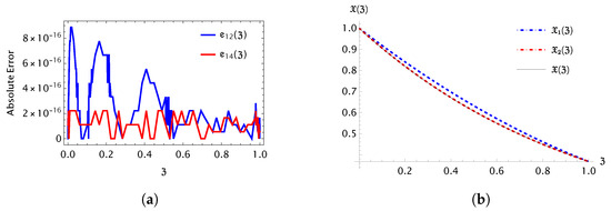
which provides us with approximated solutions that match the exact solution with a precision of at for various values, as shown in Table 1. Table 2 presents a comparison between GSJCOPMM and the three methods in [36,37,38]. Figure 1 presents the computed errors and approximate solutions. Based on the given orders of convergence , it is apparent see that the convergence rate improves as increases; a higher order of convergence means that the error goes down faster.
Table 1.
Computed errors in Example 2.
Table 2.
A comparison of approaches [36,37,38] and for Example 2 using .
Figure 1.
Figures of and for Example 2 using various with and . (a) Errors plots and . (b) Exact and approximate solutions and .
Problem 3.
for which the exact solution is . Applying the algorithm leads to
Table 3 displays the MAE for some values of , , and ε, while Table 4 displays a comparison between the , QBSM [39], and NCBS methods [40]. Figure 2a shows at . In addition, Figure 2b shows the log-errors for various and . This shows that the solutions are stable and converging.
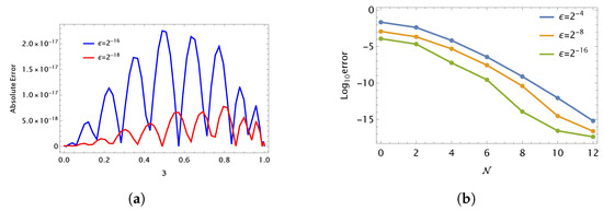
Consider the following self-adjoint singularly perturbed singular BVP [39,40]:
Table 3.
Computed MAE in Example 3.
Table 4.
Comparison of approaches [39,40] and for Example 3 using .
Figure 2.
Figures of using various for Example 3 with and . (a) for . (b) Graph of against .
Problem 4.
For one-dimensional Bratu’s problems [41]
with the exact solution in the form from [42] (Equation 47), we have
where θ satisfies . Bratu’s problems have either no solution, one solution, or two solutions, respectively, when or where . The relations between λ and θ for some values of are provided in [42] (Table 1).
Application of leads to the obtained approximated solutions matching the exact solution with a precision of at for various values, as shown in Table 5. According to Tables 1 and 2 presented in [41], Table 6 presents a comparison between the absolute errors obtained by the method and the three Schemes(15), (16)a, and (16)b in [41] as well as a computational time (CPU time) comparison between and the three finite difference Schemes(15), (16)a, and (16)b.
Table 5.
Computed errors in Example 4 when .
Table 6.
A comparison of approaches [41] and for Example 4 using and .
Remark 1.
It is important to note that the comparison of the computational time of the numerical method of with the finite difference methods shown in Example 4 shows that is faster; however, this result cannot be generalized, as the computational time may vary depending on the problem, the complexity of the equations, and the implementation details.
7.2. Numerical Simulations for Handling VOFDE (2) with BCs (3)
Problem 5.
Consider the boundary Bagely–Torvik equation [10,43]
for which the exact solution is . Applying leads to
where and .
Remark 2.
It is worth noting that , while according to the author of [10], at we obtain using . Furthermore, the authors of [43] achieved the best error of at .
Problem 6.
Consider the equation [44,45]:
with the exact solution , where . Applying using yields
Remark 3.
It is worth noting that , while according to the author of [44] is obtained using . Furthermore, the authors of [45] achieved the best error of .
Problem 7.
Consider the nonlinear differential equation
where . The exact solution is . Applying using yields
where .
Problem 8.
Consider the nonlinear BVP
where is computed such that . Applying the algorithm leads to
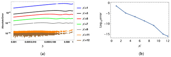
Table 7 displays the computed errors and for some values of , and . The two figures in Figure 3a,b show and for various , respectively. This shows that the solutions are stable and converging.
Table 7.
Computed errors in Example 8.
Figure 3.
Figures of using various for Example 8 with and . (a) plots for . (b) Graph of against .
8. Conclusions
Our study has introduced a novel and efficient numerical approach for solving problems involving ODEs and VOFDEs associated with BCs. The main achievements of our research can be summarized as follows:
- (i)
- We have established a solid theoretical foundation by constructing OMs and incorporating them into the SCM. This framework allows for reliable and precise numerical computation of solutions to problems described by the aforementioned ODEs and VOFDEs with BCs.
- (ii)
- Extensive error analysis and convergence studies have been conducted, providing theoretical guarantees for the effectiveness and reliability of our proposed method, known as GSJCOPMM.
Our research has significant implications, as GSJCOPMM provides several advantages over existing approaches for solving ODEs and VOFDEs with BCs. First, GSJPs ensure that the given BCs are satisfied, resulting in improved numerical solution accuracy. Second, the developed OMs and their implementation within the SCM enable efficient computations, reducing computational costs while maintaining high accuracy. These features make GSJCOPMM particularly well suited for solving complex problems encountered in various scientific and engineering fields.
The potential applications of our proposed method are broad, encompassing a wide range of problems involving ODEs and VOFDEs. Our proposed method has a broad range of potential applications involving PDEs, systems of ODEs and VOFDEs in thhe mathematical modeling of physical systems, heat transfer, boundary layer problems in fluid mechanics, the motion of mass–spring systems, reaction rates, and other phenomena characterized by these models. In conclusion, this research contributes significantly to the advancement of numerical methods for ODEs and VOFDEs with BCs, providing an efficient and accurate approach for solving complex boundary value problems. The establishment of a theoretical foundation together with the demonstrated advantages of GSJCOPMM opens up new avenues for tackling challenging problems in various scientific and engineering domains.
Funding
No funding was received to assist with the preparation of this manuscript.
Data Availability Statement
No data are associated with this research.
Acknowledgments
The author acknowledges the valuable contributions of the anonymous reviewers and editor, whose insightful comments and recommendations greatly improved the quality of this research.
Conflicts of Interest
The author declares no conflicts of interest.
Abbreviations
The following abbreviations are used in this manuscript:
| Abbreviations | Definitions |
| DEs | Differential equations |
| ODEs | Ordinary differential equations |
| PDEs | Partial differential equations |
| ODs | Ordinary derivatives |
| VOFDEs | Variable-order fractional differential equations |
| VOFDs | Variable-order fractional derivatives |
| MTVOFDEs | Multiterm variable-order fractional differential equations |
| OMs | Operational matrices |
| SCM | Spectral collocation method |
| VOFC | Variable-order fractional calculus |
| JPs | Jacobi polynomials |
| GSJPs | Generalized shifted Jacobi polynomials |
| BVPs | Boundary value problems |
| BCs | Boundary conditions |
| MAE | Maximum absolute error |
References
- Bagley, R.L.; Torvik, P.J. Fractional calculus in the transient analysis of viscoelastically damped structures. Aiaa J. 1985, 23, 918–925. [Google Scholar] [CrossRef]
- Davies, A.R.; Karageorghis, A.; Phillips, T.N. Spectral Galerkin methods for the primary two-point boundary value problem in modelling viscoelastic flows. Int. J. Numer. Methods Eng. 1988, 26, 647–662. [Google Scholar] [CrossRef]
- Karageorghis, A.; Phillips, T.N.; Davies, A.R. Spectral collocation methods for the primary two-point boundary value problem in modelling viscoelastic flows. Int. J. Numer. Methods Eng. 1988, 26, 805–813. [Google Scholar] [CrossRef]
- Baillie, R.T. Long memory processes and fractional integration in econometrics. J. Econom. 1996, 73, 5–59. [Google Scholar] [CrossRef]
- Mainardi, F. Fractional Calculus: Some Basic Problems in Continuum and Statistical Mechanics; Springer: Berlin/Heidelberg, Germany, 1997. [Google Scholar]
- Rossikhin, Y.A.; Shitikova, M.V. Applications of fractional calculus to dynamic problems of linear and nonlinear hereditary mechanics of solids. Appl. Mech. Rev. 1997, 50, 15–66. [Google Scholar] [CrossRef]
- Chow, T.S. Fractional dynamics of interfaces between soft-nanoparticles and rough substrates. Phys. Lett. A 2005, 342, 148–155. [Google Scholar] [CrossRef]
- Gregus, M. Third Order Linear Differential Equations; Springer Science & Business Media: Berlin/Heidelberg, Germany, 2012; Volume 22. [Google Scholar]
- Ahmed, H.M. Enhanced shifted Jacobi operational matrices of derivatives: Spectral algorithm for solving multiterm variable-order fractional differential equations. Bound. Value Probl. 2023, 2023, 108. [Google Scholar] [CrossRef]
- Ahmed, H.M. A new first finite class of classical orthogonal polynomials operational matrices: An application for solving fractional differential equations. Contemp. Math. 2023, 4, 974–994. [Google Scholar] [CrossRef]
- Abd-Elhameed, W.M.; Ahmed, H.M.; Youssri, Y.H. A new generalized Jacobi Galerkin operational matrix of derivatives: Two algorithms for solving fourth-order boundary value problems. Adv. Differ. Equ. 2016, 2016, 22. [Google Scholar] [CrossRef]
- Abd-Elhameed, W.M.; Al-Harbi, M.S.; Amin, A.K.; Ahmed, H.M. Spectral treatment of high-order Emden-Fowler equations based on modified Chebyshev polynomials. Axioms 2023, 12, 99. [Google Scholar] [CrossRef]
- Tural-Polat, S.N.; Dincel, A.T. Numerical solution method for multi-term variable order fractional differential equations by shifted Chebyshev polynomials of the third kind. Alex. Eng. J. 2022, 61, 5145–5153. [Google Scholar] [CrossRef]
- Ahmed, H.M. Numerical solutions for singular Lane-emden equations using shifted Chebyshev polynomials of the first kind. Contemp. Math. 2023, 4, 132–149. [Google Scholar] [CrossRef]
- Abd-Elhameed, W.M.; Ahmed, H.M. Tau and Galerkin operational matrices of derivatives for treating singular and Emden-Fowler third-order-type equations. Int. J. Mod. Phys. C 2022, 33, 2250061. [Google Scholar] [CrossRef]
- Sweilam, N.H.; Nagy, A.M.; El-Sayed, A.A. On the numerical solution of space fractional order diffusion equation via shifted Chebyshev polynomials of the third kind. J. King Saud Univ. Sci. 2016, 28, 41–47. [Google Scholar] [CrossRef]
- Liu, C.-S.; Li, B. Solving the fourth-order nonlinear boundary value problem by a boundary shape function method. Can. J. Phys. 2022, 101, 248–256. [Google Scholar] [CrossRef]
- El-Sayed, A.A.; Baleanu, D.; Agarwal, P. A novel Jacobi operational matrix for numerical solution of multi-term variable-order fractional differential equations. J. Taibah Univ. Sci. 2020, 14, 963–974. [Google Scholar] [CrossRef]
- Ahmed, H.M. New Generalized Jacobi Galerkin operational matrices of derivatives: An algorithm for solving multi-term variable-order time-fractional diffusion-wave equations. Fractal Fract. 2024, 8, 68. [Google Scholar] [CrossRef]
- Abd-Elhameed, W.M.; Alkenedri, A.M. Spectral solutions of linear and nonlinear bvps using certain Jacobi polynomials generalizing third-and fourth-kinds of Chebyshev polynomials. Comput. Model Eng. Sci. 2021, 126, 955–989. [Google Scholar] [CrossRef]
- Doha, E.H.; Abd-Elhameed, W.M.; Bhrawy, A.H. New spectral-Galerkin algorithms for direct solution of high even-order differential equations using symmetric generalized Jacobi polynomials. Collect. Math. 2013, 64, 373–394. [Google Scholar] [CrossRef]
- Bhrawy, A.H.; Abd-Elhameed, W.M. New algorithm for the numerical solutions of nonlinear third-order differential equations using Jacobi-Gauss collocation method. Math. Probl. Eng. 2011, 2011, 837218. [Google Scholar] [CrossRef]
- Ahmed, H.M. Numerical solutions of Korteweg-de Vries and Korteweg-de Vries-Burger’s equations in a Bernstein polynomial basis. Mediterr. J. Math. 2019, 16, 102. [Google Scholar] [CrossRef]
- Ahmed, H.M. Numerical solutions of high-order differential equations with polynomial coefficients using a Bernstein polynomial basis. Mediterr. J. Math. 2023, 20, 303. [Google Scholar] [CrossRef]
- Mittal, R.C.; Pandit, S. New scale-3 Haar Wavelets algorithm for numerical simulation of second order ordinary differential equations, Proceedings of the National Academy of Sciences. India Sect. Phys. Sci. 2019, 89, 799–808. [Google Scholar]
- Sharma, D.; Jiwari, R.; Kumar, S. Numerical solution of two point boundary value problems using Galerkin-finite element method. Int. J. Nonlinear Sci. 2012, 13, 204–210. [Google Scholar]
- Abd-Elhameed, W.M.; Youssri, Y.H.; Amin, A.K.; Atta, A.G. Eighth-kind Chebyshev polynomials collocation algorithm for the nonlinear time-fractional generalized Kawahara equation. Fractal Fract. 2023, 7, 652. [Google Scholar] [CrossRef]
- Youssri, Y.H.; Atta, A.G. Spectral collocation approach via normalized shifted Jacobi polynomials for the nonlinear Lane-Emden equation with fractal-fractional derivative. Fractal Fract. 2023, 7, 133. [Google Scholar] [CrossRef]
- Amin, A.Z.; Abdelkawy, M.A.; Solouma, E.; Al-Dayel, I. A Spectral Collocation Method for Solving the Non-Linear Distributed-Order Fractional Bagley–Torvik Differential Equation. Fractal Fract. 2023, 7, 780. [Google Scholar] [CrossRef]
- Chen, Y.M.; Liu, L.Q.; Li, B.F.; Sun, Y. Numerical solution for the variable order linear cable equation with Bernstein polynomials. Appl. Math. Comput. 2014, 238, 329–341. [Google Scholar] [CrossRef]
- Liu, J.; Li, X.; Wu, L. An operational matrix of fractional differentiation of the second kind of Chebyshev polynomial for solving multiterm variable order fractional differential equation. Math. Probl. Eng. 2016, 2016, 7126080. [Google Scholar] [CrossRef]
- Almeida, R.; Tavares, D.; Torres, D.F.M. The Variable-Order Fractional Calculus of Variations; Springer: Cham, Switzerland, 2019. [Google Scholar]
- Coimbra, C.F.M. Mechanics with variable-order differential operators. Ann. Phys. 2003, 515, 692–703. [Google Scholar] [CrossRef]
- Szeg, G. Orthogonal Polynomials, 4th ed.; American Mathematical Society: Providence, RI, USA, 1975; Volume XXIII. [Google Scholar]
- Luke, Y.L. Mathematical Functions and Their Approximations; Academic Press: London, UK, 1975. [Google Scholar]
- Wazwaz, A.-M. The numerical solution of sixth-order boundary value problems by the modified decomposition method. Appl. Math. Comput. 2001, 118, 311–325. [Google Scholar] [CrossRef]
- Noor, M.A.; Mohyud-Din, S.T. Homotopy perturbation method for solving sixth-order boundary value problems. Comput. Math. Appl. 2008, 55, 2953–2972. [Google Scholar] [CrossRef]
- Gul, M.; Khan, H.; Ali, A. The solution of fifth and sixth order linear and non linear boundary value problems by the improved residual power series method. JMAM 2022, 3, 1–14. [Google Scholar]
- Mishra, H.K.; Saini, S. Quartic B-Spline method for solving a singular singularly perturbed third-order boundary value problems. Am. J. Numer. Anal. 2015, 3, 18–24. [Google Scholar]
- Iqbal, M.K.; Abbas, M.; Wasim, I. New cubic B-spline approximation for solving third order Emden–Flower type equations. Appl. Math. Comput. 2018, 331, 319–333. [Google Scholar] [CrossRef]
- Adewumi, A.O.; Aderogba, A.A.; Akindeinde, S.O.; Fabelurin, O.O.; Lebelo, R.S. Finite difference spectral collocation schemes for the solutions of boundary value problems. Heliyon 2024, 10, E23453. [Google Scholar] [CrossRef] [PubMed]
- Mickens, R.E. Advances in the Applications of Nonstandard Finite Diffference Schemes; World Scientific: Singapore, 2005. [Google Scholar]
- Al-Mdallal, Q.M.; Syam, M.I.; Anwar, M.N. A collocation-shooting method for solving fractional boundary value problems. Commun. Nonlinear Sci. Numer. Simul. 2010, 15, 3814–3822. [Google Scholar] [CrossRef]
- Abdelkawy, M.A.; Lopes, A.M.; Babatin, M.M. Shifted fractional Jacobi collocation method for solving fractional functional differential equations of variable order. Chaos Solit. Fractals 2020, 134, 109721. [Google Scholar] [CrossRef]
- Yang, J.; Yao, H.; Wu, B. An efficient numerical method for variable order fractional functional differential equation. Appl. Math. Lett. 2018, 76, 221–226. [Google Scholar] [CrossRef]
Disclaimer/Publisher’s Note: The statements, opinions and data contained in all publications are solely those of the individual author(s) and contributor(s) and not of MDPI and/or the editor(s). MDPI and/or the editor(s) disclaim responsibility for any injury to people or property resulting from any ideas, methods, instructions or products referred to in the content. |
© 2024 by the author. Licensee MDPI, Basel, Switzerland. This article is an open access article distributed under the terms and conditions of the Creative Commons Attribution (CC BY) license (https://creativecommons.org/licenses/by/4.0/).