Fractal Operators and Convergence Analysis in Fractional Viscoelastic Theory

Abstract

This study delves into the convergence of operators and the viscoelastic properties of fractal ladder and tree structures. It proves the convergence of fractal stiffness operators through operator algebra, revealing a fundamental connection between operator sequence limits and fractal operator algebraic equations. Our findings demonstrate that, as the hierarchical levels of these structures increase, their viscoelastic responses increasingly align with the fractional viscoelastic behavior observed in infinite-level fractal structures. We explore the similarity in creep and relaxation behaviors between fractal ladders and trees, emphasizing the emergence of ultra-long characteristic times in steady-state creep and pronounced tailing effects in relaxation curves. This research provides novel insights into the design of fractional-order viscoelastic structures, presenting significant implications for materials science and mechanical engineering.

1. Introduction

This paper delves into the viscoelastic mechanics of fractal structures, prompted by the growing use of polymers [1,2,3], rubber [4], hydrogels [5], biological tissues [6], and composite materials [7]. These advancements have spurred deeper analysis of these materials’ mechanical properties and the evolution of viscoelastic mechanical theories.

Kelvin’s mid-19th-century discovery of zinc’s viscoelastic properties marked the beginning of viscoelastic theory [8]. Maxwell’s subsequent introduction of viscosity for all bodies [9], along with the efforts of Meyer [10] and Boltzmann [11], laid the foundations of linear viscoelasticity. The early 20th century saw further advancements by Volterra [12], who developed a mathematical theory for anisotropic solids, propelling viscoelastic mechanics forward.

Viscoelastic materials are commonly divided into two broad categories: linear and nonlinear. Linear viscoelastic materials exhibit a combination of elastic and ideal viscous behaviors, acting as an intermediate state between the elastic Hookean solid and the ideal viscous Newtonian fluid [13]. In these materials, the relationship between stress and strain changes over time, yet the stress–strain relationship remains linear at any given moment. In contrast, the mechanical behavior of nonlinear viscoelastic materials is much more complex, encompassing nonlinear elasticity, non-Newtonian fluid behavior, or a combination of both. Since the mid-20th century, there has been rapid progress in the development of constitutive theories and rheology for nonlinear viscoelastic materials [14].

The complexity of nonlinear viscoelastic behavior led researchers to propose self-similar viscoelastic models, comprising infinite elements [15], such as Schiessel et al. [16,17] and Heymans et al. [18,19]. In analyzing these models, two main approaches are predominantly used: one involves studying the complex modulus of the model within the complex domain [18,19], and the other establishes stress–strain relationships at each node, solving them with the help of matrix operations [20]. Both methods, while computationally intensive, often do not directly convey structural information. Recently, scholars introduced the theories of operational calculus and operator algebra, achieving succinct and direct results [21].

Nevertheless, prior studies [13,21,22,23,24,25,26] have proceeded under the unverified assumption that the physical fractal entities under investigation exhibit self-similarity throughout their structure, thus guiding the computation of the overall response through the formulation of stiffness operator algebraic equations. Such dependence on fractal-based reasoning, however, lacks theoretical validation of its accuracy. To enhance and refine this methodology, the present paper leverages the operational calculus and operator algebra theories to rigorously demonstrate its suitability.

Moreover, the nascent stage of operator algebra theory previously left researchers unable to fully interpret operator expression outcomes, compelling them to rely on approximation techniques, such as asymptotic expansions in Ref. [23], for their research. We have advanced the theories of operational calculus and operator algebra, integrating them with integral transforms to devise the operator kernel function (OKF) method [27]. This approach has allowed us to revisit fractional viscoelastic models, develop algebraic equations for stiffness and compliance operators for self-similar fractal structures, and finally derive functional expressions.

By comparing the OKF with Boltzmann’s superposition principle, we have established a link between the kernel function and quasi-static behavior, i.e., the relaxation function and the creep function, thus offering new insights into the viscoelastic behavior of fractal structures and highlighting the significant potential of fractal operators in simplifying the computational complexity associated with analyzing viscoelastic materials.

The organization of this paper is as follows: Section 2 utilizes operator algebra to prove the convergence of operators in fractal trees and ladders. Section 3 delineates the transformational relationships between fractal operators and the creep function or the relaxation function, highlighting the differences that set operator theory apart from classical viscoelasticity. Section 4 explores the discretization of continuous media, illustrating the standard approach to resolving fractal stiffness operators. Through this structured exposition, we bridge the gap between the fractal mechanics and conventional viscoelastic principles, offering a holistic framework that enriches our grasp and application of fractal operator theory within materials science.

2. Convergence Analysis of Viscoelastic Fractal Operators

2.1. Stiffness Operator Method and Compliance Operator Method

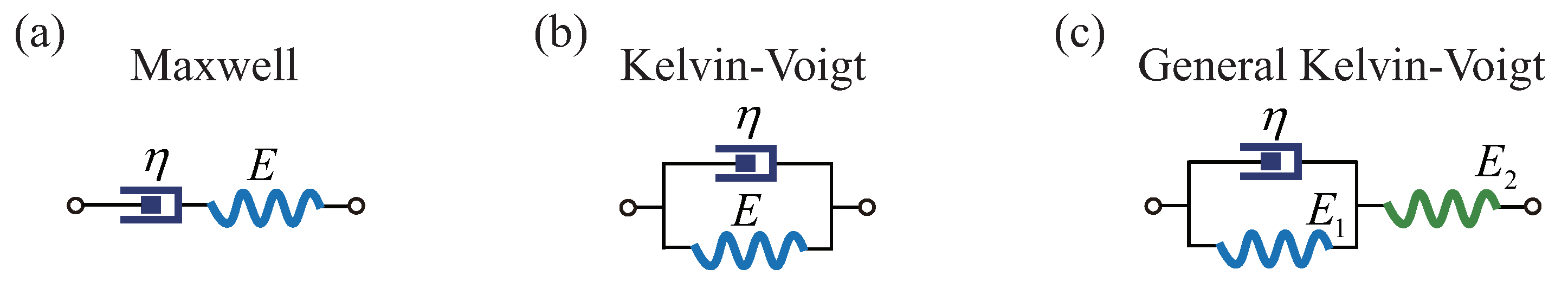
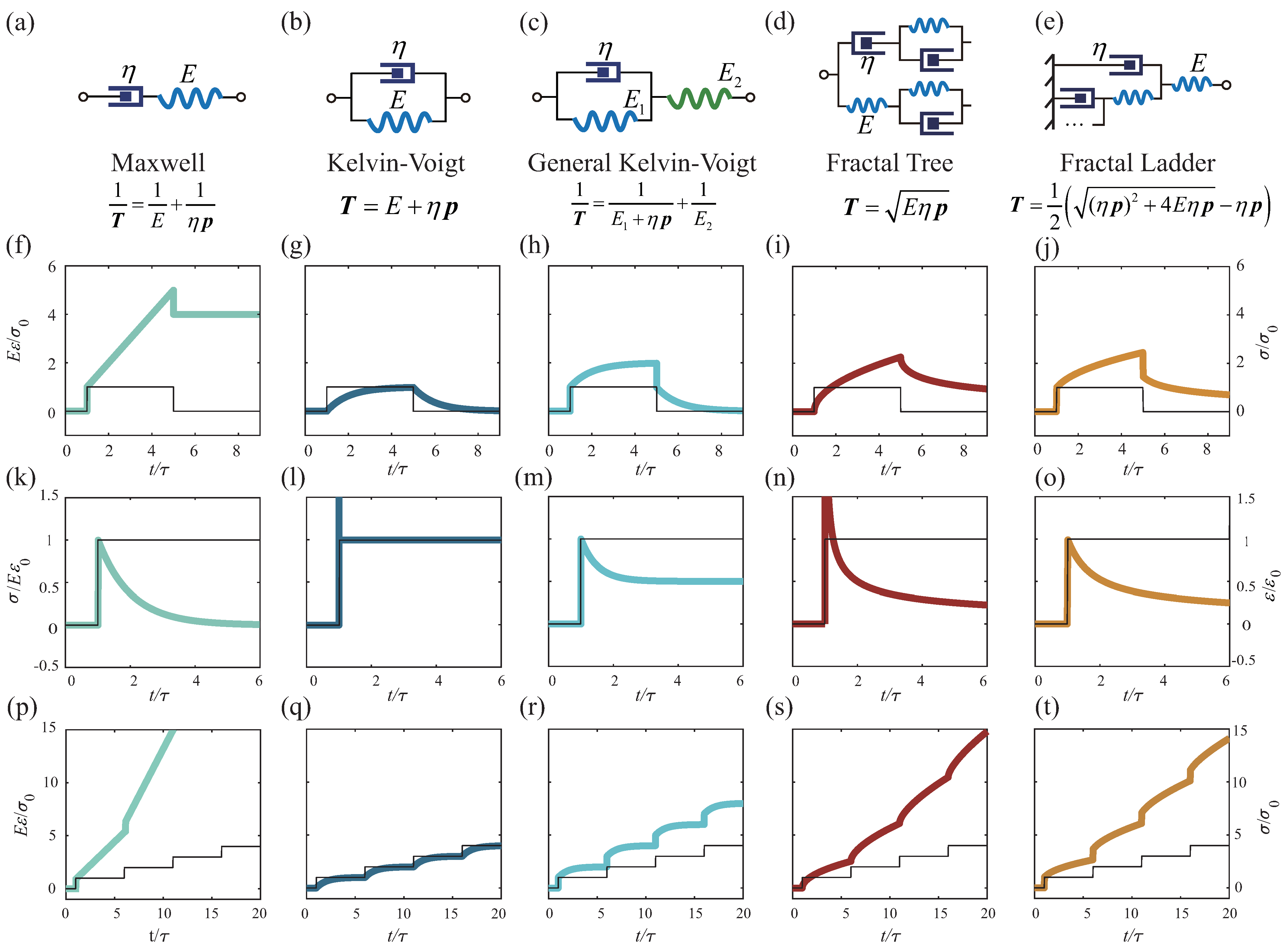
Linear viscoelastic materials, representing synergy between elasticity and perfect viscosity, serve as a transitional phase bridging the gap between the elastic behavior of Hookean solids and the ideal viscosity of Newtonian fluids, with several classic viscoelastic models illustrated in Figure 1.

Establishing a structure’s total constitutive relationship demands the amalgamation of stress-based equilibrium equations, strain-based compatibility equations, and the distinct constitutive relations for each element. The methodology for solving this comprehensive set of differential equations to ascertain the constitutive equation in a unidimensional framework is elaborated upon in Appendix A.

This method is viable for viscoelastic models constituted by a finite ensemble of elements. Nonetheless, with an increase in the number of elements, there is a proportional rise in the number of unknowns and equations, consequently amplifying computational complexity. In scenarios involving models with an infinite array of elements, the infinite count of unknowns renders this computational strategy untenable.

Hu et al. [13] pioneered the application of operator algebra to non-Newtonian fluid dynamics, utilizing force–electricity analogies to elucidate the stress–strain relationships inherent in viscoelastic materials. This innovative methodology has since been adopted by various researchers to explore a wide range of topics, including the viscoelastic properties of ligaments [22], the spiking and propagation of neural electrical signals [23], the complex dynamics of blood flow within the infinite elastic cavity model [25], and the intricate mechanical behaviors of bone [26]. Herein, we offer a concise review of this method.

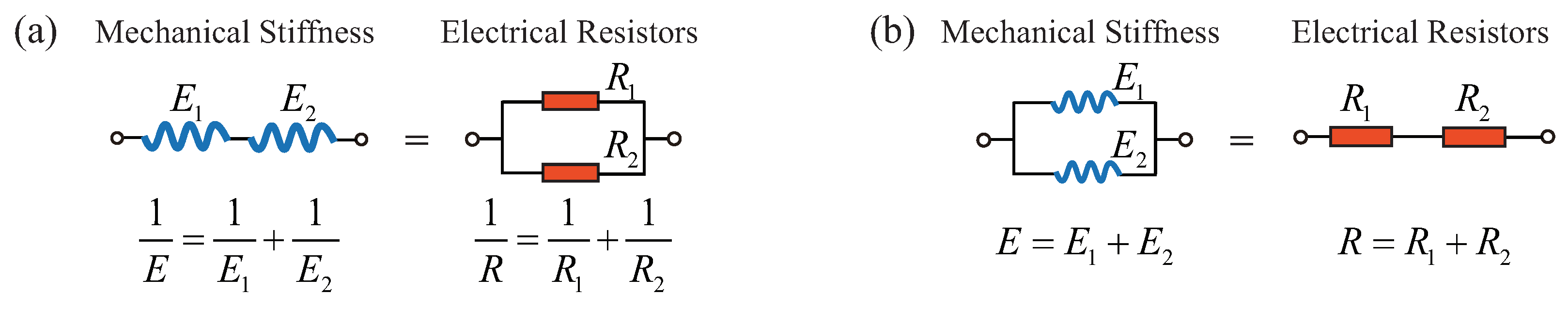
Leveraging the concept of the force–electricity analogy, the integration of two mechanical elements in series results in a combined stiffness analogous to the parallel configuration of electrical resistors within a circuit. Similarly, their cumulative compliance corresponds to the series arrangement of resistors. Conversely, the parallel coupling of mechanical elements yields a composite stiffness akin to resistors in series, whereas their collective compliance mirrors the parallel arrangement of resistors. This correlation is visually depicted and clarified in Figure 2.

In the subsequent sections, we will adopt an operator-based framework where stiffness is expressed through operators, termed the stiffness operator method (SOM), and compliance is articulated in a similar manner, denoted as the compliance operator method (COM). This paper primarily focuses on thoroughly exploring and elucidating the stiffness operator methodology.

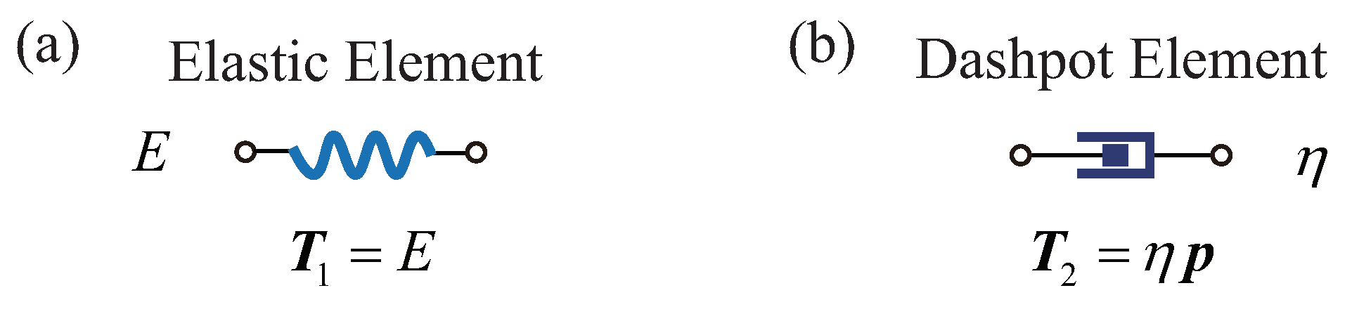
This study explores the viscoelastic behavior of models comprising energy-storing components, symbolized by springs, and energy-dissipating components illustrated by dashpots, as demonstrated in Figure 3. The stiffness operators for the springs ${\mathit{T}}_1$ and for the dashpots ${\mathit{T}}_2$ are represented as

$$\begin{array}{c}\hfill {\mathit{T}}_1=E,{\mathit{T}}_2=\eta \mathit{p}.\end{array}$$

(1)

where $\mathit{p}=\frac{\mathrm{d}}{\mathrm{d}\mathrm{t}}$ denotes the Heaviside operator, E denotes the elastic module of the spring, and $\eta$ denotes the coefficient of viscosity.

Utilizing this method enables the swift calculation of the stiffness operator for the Maxwell model as follows:

$$\begin{array}{c}\hfill {\mathit{T}}_{Maxwell}=\frac{E\eta \mathit{p}}{E+\eta \mathit{p}}.\end{array}$$

(2)

The stiffness operator for the Kelvin–Voigt model is defined as

$$\begin{array}{c}\hfill {\mathit{T}}_{KV}=E+\eta \mathit{p}.\end{array}$$

(3)

Similarly, the stiffness operator for the GKV model is determined as

$$\begin{array}{c}\hfill {\mathit{T}}_{GKV}=\frac{(E_1+\eta \mathit{p})E_2}{E_1+E_2+\eta \mathit{p}}.\end{array}$$

(4)

Appendix A provides a guide to employing stiffness operators for determining the functional relationship between stress and strain in these models.

2.2. Algebraic Equations of Stiffness Operators for Fractal Cells

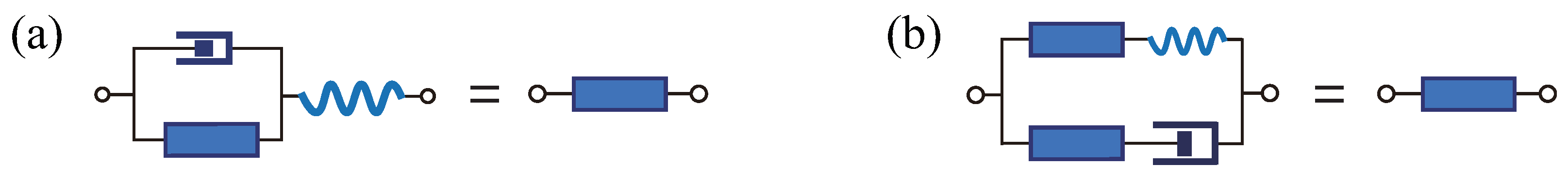
This section revisits the application of the SOM to fractal cells, as depicted in Figure 4. The figure demonstrate that a fractal tree or ladder, viewed in its entirety, matches a single fractal cell (as depicted on the left-hand side in Figure 4a,b); similarly, these structures can also be equated to a fractal element (as shown on the right-hand side in Figure 4a,b). Utilizing this equivalence, algebraic equations for stiffness operators are formulated. Solving these equations yields precise operator expressions for both fractal ladders and trees, thus providing a structured approach for analyzing their mechanical properties.

For the fractal ladder structure, see Figure 4a; based on the equivalence of compliance, we have

$$\begin{array}{c}\hfill \frac{1}{\mathit{T}}=\frac{1}{E}+\frac{1}{\mathit{T}+\eta \mathit{p}}.\end{array}$$

(5)

In Equation (5), the left side represents the compliance operator of the fractal element, while the right side corresponds to the compliance operator of the fractal cell. Equation (5) forms a quadratic algebraic equation of operators. Solving Equation (5) and considering the condition for positive stiffness [24,28,29,30], we obtain the operator for the fractal ladder:

$$\begin{array}{c}\hfill \mathit{T}=\sqrt{\frac{{(\eta \mathit{p})}^2}{4}+E\eta \mathit{p}}-\frac{\eta \mathit{p}}{2}.\end{array}$$

(6)

For the fractal tree structure, see Figure 4b; based on the equivalence of stiffness, we have

$$\begin{array}{c}\hfill \mathit{T}=\frac{E\mathit{T}}{\mathit{T}+E}+\frac{\eta \mathit{pT}}{\mathit{T}+\eta \mathit{p}},\end{array}$$

(7)

In Equation (7), the left side represents the stiffness operator of the fractal element, while the right side corresponds to the stiffness operator of the fractal cell. Equation (7) is a quadratic algebraic equation of operators. Solving Equation (7) and considering the condition for positive stiffness [24,30] yields the operator for the fractal tree:

$$\begin{array}{c}\hfill \mathit{T}=\sqrt{E\eta \mathit{p}}.\end{array}$$

(8)

Remark 1.

From a mathematical perspective, both Equations (5) and (7) are expected to have two radical results [28,29,30]. Indeed, earlier research by Yin et al. [24] has shown that an nth-order operator algebra equation should have at least n solutions in more general circumstances. However, for the specific issue considered in this paper, the relationship between stress and strain is represented as $\sigma (t)=\mathit{T}\epsilon (t)$, indicating that an increase in positive strain applied to the structure should cause increased stress in the same direction. Given that the action of operators is realized through the convolution of the operator kernel function with the input, it necessitates that the structure’s kernel function be positive, which also implies that the stiffness operator must be positive. Therefore, only the positive roots of Equations (6) and (8) have been retained.

This section delves deeper into the operator expressions for fractal ladders and trees, with a focus on Equations (6) and (8). We unravel how these structures respond to a given stimulus, revealing a fundamental similarity in their behavior: both are characterized by quadratic radical operators, underscoring their non-rational nature. Yet, a striking divergence emerges in their complexity. The operator for the fractal tree is remarkably straightforward, a reflection of its symmetrical topology. In contrast, the operator for the fractal ladder exhibits greater complexity due to the disruption of this symmetry. This contrast not only highlights the distinctive architectural influences on their mechanical responses but also enriches our understanding of their intrinsic properties, offering a nuanced perspective on the dynamics of fractal-based structures.

2.3. The Logical Foundation of the Equivalence Postulate

In the preceding analysis, an implicit assumption of equivalence was introduced such that

fractal elements ≈ fractal trees or ladder ≈ fractal cells.

This perception, more intuitive than deductive, lays the groundwork for formulating algebraic equations specific to fractal operators. Closer scrutiny of these equations unveils an underlying presumption: the existence of stiffness operators for fractal ladders and trees. Our approach progresses by first positing the existence of fractal operators, then using this equivalence to derive the relevant algebraic equations, and finally solving these equations to construct the fractal operators. This methodology combines intuitive reasoning with analytical rigor to unravel the intricacies of fractal mechanics.

While this approach is standard for structures with a finite hierarchy, the premise becomes less clear when dealing with fractal structures of infinite levels. Appendix B explores the generalized Maxwell model, which is derived by arranging infinitely many Maxwell models in parallel. This approach results in paradoxes, rendering the model unsolvable. Hence, this indicates that methodologies effective for finite structures may not extend straightforwardly to infinite ones, highlighting the need for a logical and robust theoretical basis for their existence.

Our investigation primarily concentrates on two pivotal structures: fractal trees and fractal ladders. The former embody symmetric fractal topology, whereas the latter illustrate a fractal topology characterized by disrupted symmetry. This distinction not only informs our understanding of fractal mechanics but also enriches our comprehension of the diversity within fractal structures.

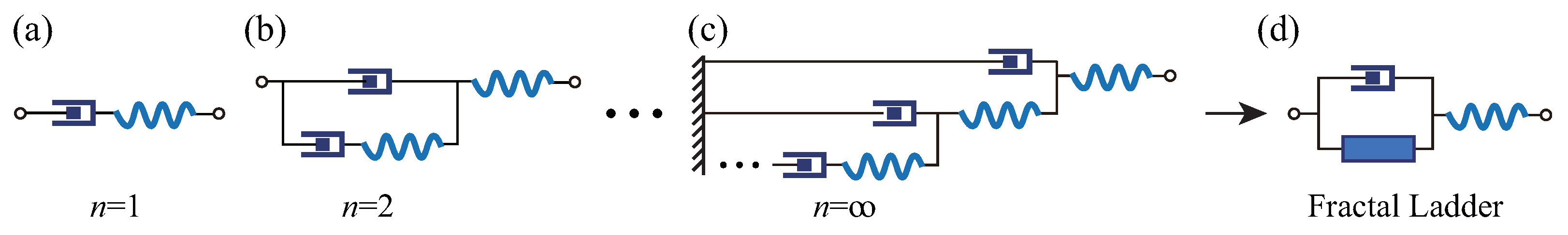
2.4. Fractal Ladder

The basic unit of the fractal ladder structure is the Maxwell element, which consists of a spring and a dashpot connected as shown in Figure 5. Due to the entire topology presenting a ladder-like configuration, when the number of structural levels approaches infinity, a fractal topology is formed; hence, the term ’fractal ladder’ is used. The fractal ladder is not a traditional geometric fractal exhibiting self-similarity but rather a self-similar physical fractal composed of identical elements.

In Figure 5, according to operator algebra, the stiffness operator of adjacent nth level structures and $(n+1)$th level structures satisfies the following recursive relationship:

$$\begin{array}{c}\hfill \frac{1}{{\mathit{T}}_n+\eta \mathit{p}}+\frac{1}{E}=\frac{1}{{\mathit{T}}_{n+1}}.\end{array}$$

(9)

Upon simplification, we can obtain

$$\begin{array}{c}\hfill {\mathit{T}}_{n+1}=\frac{({\mathit{T}}_n+\eta \mathit{p})E}{{\mathit{T}}_n+\eta \mathit{p}+E}.\end{array}$$

(10)

Similar to the fractal tree structure, we will now prove that the sequence of operators constituting the fractal ladder structure converges to a limit.

Proof. 

The stiffness operators for the first- and second-level structures are, respectively, represented as

$$\begin{array}{c}\hfill {\mathit{T}}_1=\frac{\eta E\mathit{p}}{\eta \mathit{p}+E},{\mathit{T}}_2=\frac{E\eta \mathit{p}\left(2E+\mathit{p}\eta \right)}{E^2+3E\eta \mathit{p}+{\eta }^2{\mathit{p}}^2}.\end{array}$$

(11)

Equation (11) can be derived to yield

$$\begin{array}{c}\hfill {\mathit{T}}_2-{\mathit{T}}_1=\frac{E^3\eta \mathit{p}}{\left(E+\eta p\right)\left(E^2+3E\eta \mathit{p}+{\eta }^2{\mathit{p}}^2\right)}>0.\end{array}$$

(12)

We thus proved that ${\mathit{T}}_2>{\mathit{T}}_1$. Assuming ${\mathit{T}}_n>{\mathit{T}}_{n-1}$, we next prove that ${\mathit{T}}_{n+1}>{\mathit{T}}_n$. Let the function $f(x)$ be

$$\begin{array}{c}\hfill f(x)=\frac{(x+\eta \mathit{p})E}{x+\eta \mathit{p}+E}=E-\frac{E^2}{x+\eta \mathit{p}+E}.\end{array}$$

(13)

Differentiating Equation (13) with respect to x yields

$$\begin{array}{c}\hfill f^{\prime }(x)=\frac{E^2}{{\left(E+x+\eta \mathit{p}\right)}^2}>0.\end{array}$$

(14)

Therefore, the function is monotonically increasing, implying $(x_2-x_1)\left[f(x_2)-f(x_1)\right]>0$. Given that ${\mathit{T}}_n>{\mathit{T}}_{n-1}$, it follows that

$$\begin{array}{c}\hfill f({\mathit{T}}_n)>f({\mathit{T}}_{n-1}).\end{array}$$

(15)

Combining Equations (10), (13) and (15), we arrive at

$$\begin{array}{c}\hfill {\mathit{T}}_{n+1}>{\mathit{T}}_n.\end{array}$$

(16)

Note that the fractal ladder, formed by connecting a spring on the outermost side in series with other structures, inherently has an equivalent stiffness lower than that of a single spring. This proposition’s validity is further supported by Equation (13):

$$\begin{array}{c}\hfill f(x)=E-\frac{E^2}{x+\eta \mathit{p}+E}<E.\end{array}$$

(17)

Therefore, the sequence of stiffness operators for the fractal ladder structure is a monotonically increasing and bounded sequence of operators. Consequently, this sequence of operators must have a limit, and $\underset{n\to \infty }{lim}{\mathit{T}}_{n+1}=\underset{n\to \infty }{lim}{\mathit{T}}_n=\mathit{T}$. □

Remark 2.

Mikusiński rigorously defined the concept of operator sequence convergence in Ref. [30]: If there exists $\tilde{\mathit{T}}\ne 0$ such that the sequence of operators $\{{\mathit{T}}_n/\tilde{\mathit{T}}\}$ has a uniformly convergent sequence of kernel functions, then the sequence of operators $\left\{{\mathit{T}}_n\right\}$ is said to converge. Furthermore, it is denoted by $\underset{n\to \infty }{lim}{\mathit{T}}_n=\tilde{\mathit{T}}\underset{n\to \infty }{lim}{\mathit{T}}_n/\tilde{\mathit{T}}$. In fact, the above proof process can be viewed as setting $\tilde{\mathit{T}}=\mathit{I}$, where $\mathit{I}$ represents the identity operator.

Taking the limit of both sides of Equation (9) yields the fractal operator algebraic Equation (5). As mentioned previously, this is a quadratic algebraic equation for the fractal operator, with a radical solution (see Equation (6)). Clearly, for the fractal ladder, the fractal operator is of a non-rational type. Its non-rationality still stems from the infinity of the fractal ladder’s structural levels.

It is verifiable that a finite-level self-similar ladder structure, once the number of structural levels exceeds three, can be replaced by an infinite-level self-similar fractal ladder. Therefore, the use of fractal operators enables not only the attainment of concise and direct results but also ensures sufficient accuracy within the characteristic time.

2.5. Fractal Tree

Figure 6 illustrates the generative process of a fractal tree, depicting the evolution from a finite-level structure to an infinite-level structure. According to the operator stiffness method, the stiffness operator of the nth level structure is related to that of the $(n+1)$th level structure through the following recursive relation:

$$\begin{array}{c}\hfill {\mathit{T}}_{n+1}=\frac{E{\mathit{T}}_n}{{\mathit{T}}_n+E}+\frac{\eta \mathit{p}{\mathit{T}}_n}{{\mathit{T}}_n+\eta \mathit{p}}.\end{array}$$

(18)

Given that the stiffness operator and the compliance operator are inversely related, taking the reciprocal of both sides of Equation (18) yields the recursive relation for the compliance operator:

$$\begin{array}{c}\hfill \frac{1}{{\mathit{T}}_{n+1}}=\frac{({\mathit{T}}_n+E)({\mathit{T}}_n+\eta \mathit{p})}{E{\mathit{T}}_n({\mathit{T}}_n+\eta \mathit{p})+\eta \mathit{p}{\mathit{T}}_n({\mathit{T}}_n+E)}.\end{array}$$

(19)

Leveraging the principle of monotonic boundedness for operator sequences, we prove the existence of a limit for the sequence of operators, specifically $\underset{n\to \infty }{lim}{\mathit{T}}_n=\mathit{T}$.

Proof. 

Firstly, we establish the boundedness of the operator sequence. During the loading process, the applied stress (strain) induces an increasing strain (stress), ensuring that the stiffness operator remains positive and, consequently, has a lower bound.

Utilizing mathematical induction, we will prove that the sequence of stiffness operators is decreasing. For the first-level structure, we have

$$\begin{array}{c}\hfill {\mathit{T}}_1=E+\eta \mathit{p}.\end{array}$$

(20)

Substituting Equation (20) into Equation (18) yields

$$\begin{array}{c}\hfill {\mathit{T}}_2=\frac{E{\mathit{T}}_1}{{\mathit{T}}_1+E}+\frac{\eta \mathit{p}{\mathit{T}}_1}{{\mathit{T}}_1+\eta \mathit{p}}=\left(E+\eta \mathit{p}\right)\left(\frac{E}{2E+\eta \mathit{p}}+\frac{\eta \mathit{p}}{E+2\eta \mathit{p}}\right).\end{array}$$

(21)

Subtracting Equation (20) from Equation (21), we obtain

$$\begin{array}{c}\hfill {\mathit{T}}_2-{\mathit{T}}_1=-\frac{\left(E+\eta \mathit{p}\right)\left(E^2+E\eta \mathit{p}+{\eta }^2{\mathit{p}}^2\right)}{\left(2E+\eta \mathit{p}\right)\left(E+2\eta \mathit{p}\right)}<0.\end{array}$$

(22)

We thus proved that ${\mathit{T}}_2<{\mathit{T}}_1$. Assuming ${\mathit{T}}_n<{\mathit{T}}_{n-1}$, we next prove that ${\mathit{T}}_{n+1}<{\mathit{T}}_n$. Let the function $f(x)$ be

$$\begin{array}{c}\hfill f(x)=\frac{Ex}{x+E}+\frac{x\eta \mathit{p}}{x+\eta \mathit{p}}.\end{array}$$

(23)

Differentiating Equation (23) results in

$$\begin{array}{c}\hfill f^{\prime }(x)=\frac{E^2}{{\left(E+x\right)}^2}+\frac{\eta {\mathit{p}}^2}{{\left(\eta \mathit{p}+x\right)}^2}>0.\end{array}$$

(24)

Therefore, the function is monotonically increasing, implying $(x_2-x_1)\left[f(x_2)-f(x_1)\right]>0$. Given that ${\mathit{T}}_n<{\mathit{T}}_{n-1}$, it follows that

$$\begin{array}{c}\hfill f({\mathit{T}}_n)<f({\mathit{T}}_{n-1}).\end{array}$$

(25)

Combining Equations (18), (23) and (25), we arrive at

$$\begin{array}{c}\hfill {\mathit{T}}_{n+1}<{\mathit{T}}_n.\end{array}$$

(26)

By immediate application of mathematical induction, it is evident that the stiffness operator decreases as the structural level n increases. Given that the stiffness operator is monotonically decreasing and bounded below, it necessarily converges to a limit as follows: $\underset{n\to \infty }{lim}{\mathit{T}}_{n+1}=\underset{n\to \infty }{lim}{\mathit{T}}_n=\mathit{T}$. □

Since the sequence of linear operators converges and has a unique limit, taking the limit of both sides of Equation (18) simultaneously yields the fractal stiffness operator Equation (7) mentioned earlier by Guo and Yin et al. [23]. As discussed, this is a quadratic algebraic equation for the fractal operator, with a radical solution. As mentioned, the radical-type fractal operator in Equation (8) is a non-rational operator.

At this point, we can make a fundamental judgment: for finite-level self-similar structures, the operator is rational; for infinite-level self-similar fractal structures, the fractal operator is non-rational. Clearly, the non-rational nature of the fractal operator arises from the infiniteness of the structural levels. The properties of rational and non-rational operators differ significantly. As outlined in Mikusinski’s work [30], kernel functions for rational operators typically manifest as elementary functions. Our earlier research confirms that kernel functions associated with non-rational operators are typically non-elementary functions.

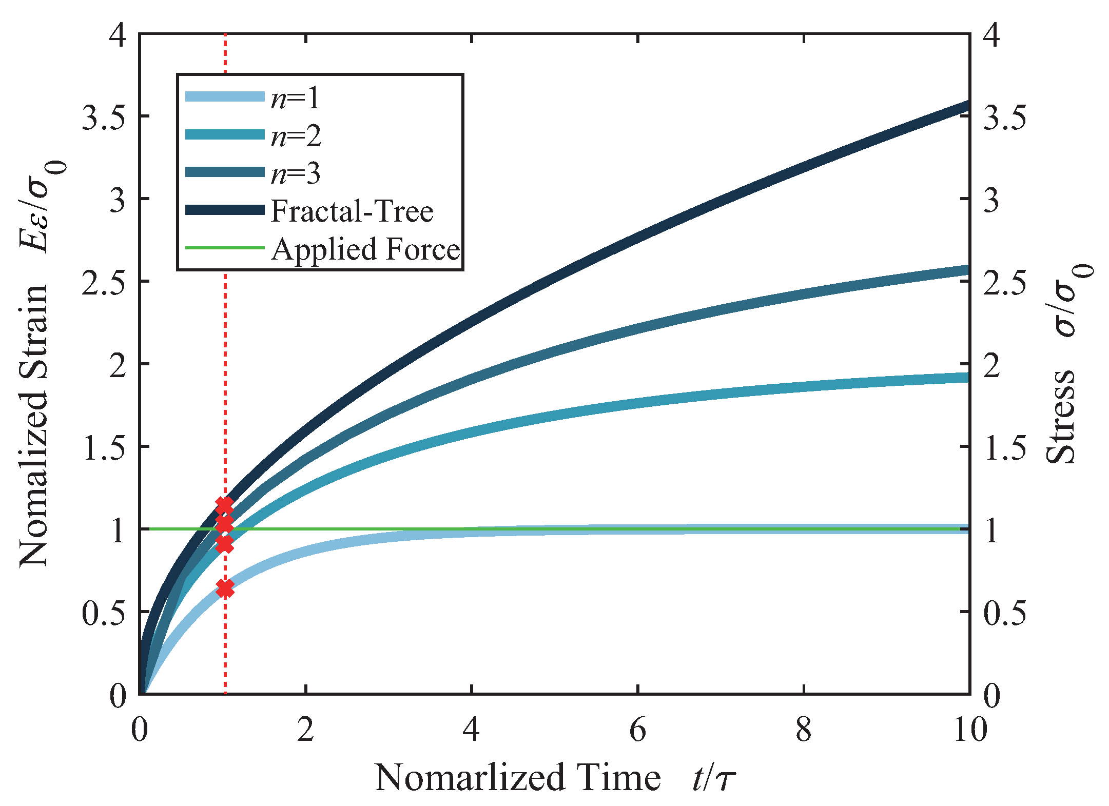
Figure 7 illustrates the creep response of structures from levels 1 to 3 compared to an infinite-level structure. With the increase in structural levels, the multi-level structure’s creep curves rapidly converge to the fractal tree within a characteristic time range, as indicated by the red dashed line. The findings suggest that, as the hierarchy of a finite-level structure extends beyond three levels, its mechanical behavior within the characteristic time can be represented by an infinite-level structure. Additionally, the analytical process for determining the behavior of an infinite-level structure proves to be simpler than for a finite-level structure, thus enhancing the model’s practical applicability in viscoelastic investigations. Moreover, the level-1 Voigt model entirely lacks the long-term relaxation effect. The greater the number of structural levels, the more pronounced the long-term relaxation effect becomes. An infinite-level fractal structure exhibits the most pronounced characteristics of ultra-long relaxation time. This discovery holds significant importance for understanding the mechanical behavior of complex viscoelastic materials.

3. Viscoelastic Response Curves of Fractal Structures

3.1. Correspondence between Operator Kernel Functions and Relaxation and Creep Functions

This section establishes a direct and intrinsic link between fractal operators and the functions governing relaxation and creep. This correlation renders fractal operators exceptionally apt for delving into the dynamics of creep and relaxation behaviors. Systems constituted by linear physical elements inherently display linearity, aligning with the Boltzmann superposition principle:

$$\begin{array}{c}\hfill \sigma (t)={\epsilon }_{0}Y(t)+{\int }_{0+}^{t}Y(t-\tilde{\tau })\frac{\mathrm{d}\epsilon (\tilde{\tau })}{\mathrm{d}\tilde{\tau }}\mathrm{d}\tilde{\tau }.\end{array}$$

(27)

$$\begin{array}{c}\hfill \epsilon (t)={\sigma }_{0}J(t)+{\int }_{0+}^{t}J(t-\tilde{\tau })\frac{\mathrm{d}\sigma (\tilde{\tau })}{\mathrm{d}\tilde{\tau }}\mathrm{d}\tilde{\tau }.\end{array}$$

(28)

In the equations, $Y(t)$ represents the material’s relaxation function, and $J(t)$ denotes the material’s creep function. Utilizing integration by parts, Equations (27) and (28) can be rewritten in a convolution form:

$$\begin{array}{c}\hfill \sigma (t)=Y(t)\ast \dot{\epsilon }(t)=\epsilon (t)\ast \dot{Y}(t).\end{array}$$

(29)

$$\begin{array}{c}\hfill \epsilon (t)=J(t)\ast \dot{\sigma }(t)=\sigma (t)\ast \dot{J}(t).\end{array}$$

(30)

Notice that both Equations (29) and (30) are convolution expressions. In fact, in Mikusinski’s monograph [30], operators are defined through convolution. This implies that convolution expressions in creep and relaxation theories often correspond to a certain fractal operator. Specifically, in Equation (29), we can consider strain as the input signal and stress as the output signal, making the creep function $J(t)$ necessarily the kernel function of some fractal stiffness operator. Similarly, the relaxation function $Y(t)$ in Equation (30) is undoubtedly the kernel function of a fractal compliance operator.

Let the stiffness operator of the viscoelastic material be denoted as $\mathit{T}$ and its compliance operator as $\frac{1}{\mathit{T}}$. Then, the viscoelastic stress–strain relationship expressed in terms of operators is

$$\begin{array}{c}\hfill \sigma (t)=\mathit{T}(\mathit{p})\epsilon (t),\mathrm{or}\epsilon (t)=\frac{1}{\mathit{T}}(\mathit{p})\sigma (t).\end{array}$$

(31)

Based on the operator kernel function theory previously discussed [27], operator operations are defined through the convolution integral of their corresponding kernel functions (generalized functions), namely

$$\begin{array}{c}\hfill \sigma (t)={\mathcal{L}}^{-1}[\mathit{T}(\mathit{p})](t)\ast \epsilon (t).\end{array}$$

(32)

$$\begin{array}{c}\hfill \epsilon (t)={\mathcal{L}}^{-1}[\frac{1}{\mathit{T}}(\mathit{p})](t)\ast \sigma (t).\end{array}$$

(33)

Comparing Equations (29) and (30) with Equations (32) and (33) yields

$$\begin{array}{c}\hfill {\mathcal{L}}^{-1}[\mathit{T}(\mathit{p})](t)=\dot{Y}(t),\mathrm{or}Y(t)={\int }_{0+}^t{\mathcal{L}}^{-1}[\mathit{T}(\mathit{p})](\tilde{\tau })\mathrm{d}\tilde{\tau }.\end{array}$$

(34)

$$\begin{array}{c}\hfill {\mathcal{L}}^{-1}[\frac{1}{\mathit{T}}(\mathit{p})](t)=\dot{J}(t),\mathrm{or}J(t)={\int }_{0+}^t{\mathcal{L}}^{-1}[\frac{1}{\mathit{T}}(\mathit{p})](\tilde{\tau })\mathrm{d}\tilde{\tau }.\end{array}$$

(35)

Equations (34) and (35) indicate that, once the stiffness or compliance operator of a structure is known, the OKF can be obtained through the inverse Laplace transform, thereby deriving the relaxation or creep function. It is important to note that the above operations only require manipulation of the stiffness or compliance operator, without involving the input and output signals.

As mentioned, the stiffness and compliance operators characterize the intrinsic properties of self-similar fractal structures themselves. By understanding the intrinsic properties within the physical fractal space, one can determine the creep and relaxation functions. This facilitates research into creep and relaxation phenomena.

3.2. Comparison of Mechanical Behavior between Several Classical Viscoelastic Models and Fractal Tree, Fractal Ladder Structures

As discussed earlier, we now summarize the relaxation and creep functions, along with the response curves under cyclic loading, for classical viscoelastic models and fractal tree and ladder structures in Figure 8.

Figure 8a–e display the schematic diagrams and corresponding stiffness/compliance operator expressions for the classical Maxwell model, Voigt model, generalized Kelvin–Voigt model, fractal tree model, and fractal ladder model. Comparing the creep response to step stress in Figure 8f–j, it is evident that fractal models significantly differ from classical models. Upon instantaneous loading, the fractal ladder structure’s end has a series spring element that produces instantaneous elastic deformation, similar to the Maxwell and three-parameter GKV models. In contrast, the fractal tree model and Voigt model, lacking an independent load-bearing structure, do not exhibit instantaneous strain. During the steady creep stage, models with a finite number of elements rapidly stabilize in deformation rate, indicating transfer of all viscous forces to the elastic el‘ements. In comparison, the elements of the infinite-level fractal model continuously transmit stress, leading to ongoing creep with a characteristic time far exceeding that of finite-level structures.

Figure 8k–o show the stress relaxation behavior to step strain. These curves reveal that the behavior of fractal structures is significantly different from finite-level models. In terms of instantaneous behavior, the fractal tree model and Voigt model exhibit a sharp increase in stress, whereas the Maxwell, GKV, and fractal ladder models, which contain independent load-bearing elastic elements, predominantly absorb instantaneous strain through these elements. For long-term relaxation, fractal structures exhibit characteristics of decaying over time and eventually tending to zero, with a gradually decreasing rate of decay, similar to the Maxwell model. Notably, fractal structures more distinctly exhibit the tailing or dragging phenomenon, prevalent in rock creep tests, indicating that fractional viscoelastic models are more effective in describing such materials.

Figure 8p–t present the response curves of the models under multiple loading conditions. From these curves, it can be observed that, due to their prolonged characteristic times, fractal models cannot disperse external forces promptly within one loading cycle and thus enter the next cycle. This characteristic indicates that the mechanical behavior exhibited by fractal structures under periodic loading more closely resembles rheological properties. This behavior reveals the uniqueness of fractal structures in handling dynamic loads, which is significant for understanding the response of such structures in practical applications.

4. Discretization of Continuous Viscoelastic Bodies into Fractal Topological Structures

Discrete fractal models, built from physical elements, showcase the intriguing ability to transition between discretization and continuity. Peng et al. [25] investigated the infinite elastic cavity model of arterial blood flow, transforming the continuous vascular wall into a myriad of microelastic cavities, crafting a physical fractal model that mirrors blood flow dynamics. Similarly, Mario Di Paola et al. [31] explored fractional viscoelastic theory, adopting the strategy of breaking continua into discrete segments. 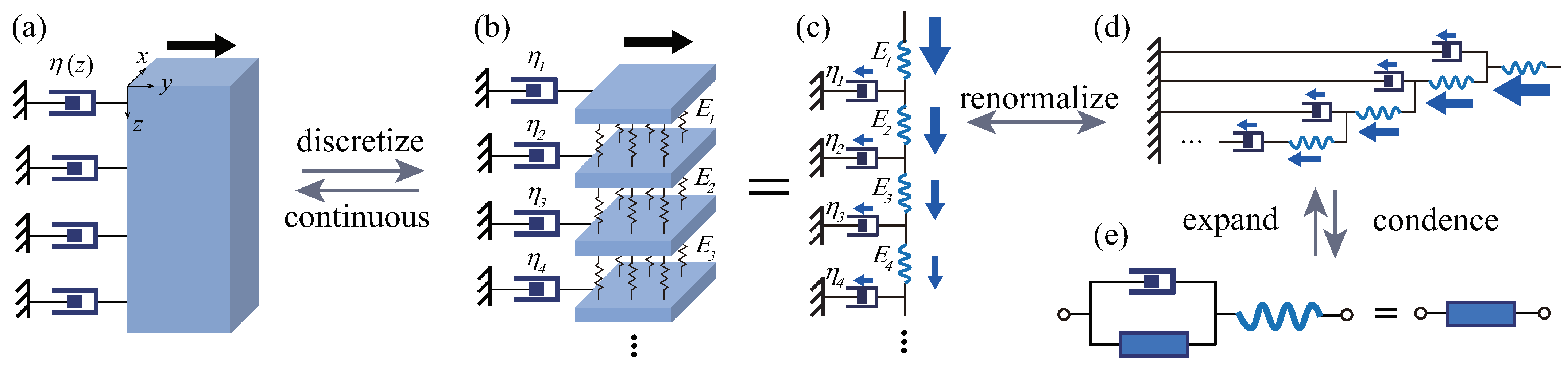This section, as illustrated by Figure 9, elucidates the process of discretizing an elastic body with distributed viscous constraints and illustrates how this approach leads to the fractalization of force transmission pathways, thereby offering a novel perspective on modeling complex physiological and material behaviors.

Figure 9a,b depict an elastic body under lateral forces at its upper boundary, experiencing shear deformation that initiates force transmission from top to bottom. By dividing the body vertically (z-direction) into thin slices (each with thickness $\Delta z$), it transitions from a continuous entity (Figure 9a) to a discrete system (Figure 9b), where slices are linked by elastic elements and to boundaries by viscous elements, allowing force to propagate through springs and dashpots. This setup leads to the multi-level self-similar model in Figure 9c: applied forces traverse internal elastic components, bifurcating at each level—one path through dashpots to boundaries and the other to subsequent elastic layers. This repetitive sequence crafts a layered mesh of elastic and viscous connections. Drawing on this model, Schiessel and Blumen [16,17], Heymans et al. [18,19], and Mario Di Paola et al. [31] introduced a pivotal transformation relationship, correlating the body’s internal elastic constants with the external viscous constraints’ viscosity coefficients by

$$\begin{array}{c}\hfill E_k=\frac{1}{2k-1}\frac{\mathsf{\Gamma }(\beta )}{\mathsf{\Gamma }(1-\beta )}\frac{\mathsf{\Gamma }(k+1-\beta )}{\mathsf{\Gamma }(k-1+\beta )}{E}_0.\end{array}$$

(36)

$$\begin{array}{c}\hfill {\eta }_k=2\frac{\mathsf{\Gamma }(\beta )}{\mathsf{\Gamma }(1-\beta )}\frac{\mathsf{\Gamma }(k+1-\beta )}{\mathsf{\Gamma }(k+\beta )}{\eta }_0.\end{array}$$

(37)

This leads to the derivation of a fractional relationship between stress and strain:

$$\begin{array}{c}\hfill \sigma (t)=\frac{{\mathrm{d}}^{\beta }}{\mathrm{d}{t}^{\beta }}\epsilon (t).\end{array}$$

(38)

It is important to note that the constraint relations between physical constants (Equations (36) and (37)) are artificially designed with the purpose of deriving the fractional viscoelastic constitutive as in Equation (38). Such an operation is not natural. Below, we provide a more intuitive explanation.

In this scenario, we imagine a structure where each level is composed of identical elements, ensuring uniform elastic constants and equal viscosity coefficients for all viscous constraints. By applying the principle of self-similarity, we can transform the model in Figure 9c into a fractal ladder configuration, as shown in Figure 9d. Remarkably, this fractal ladder mirrors the topology of the ladder in Figure 5 exactly. Moving forward, we abstract the fractal cell from the ladder, and, by developing and resolving the algebraic equation for the fractal stiffness operator (mirroring Equation (5)), we arrive at the fractal operator expression (aligned with Equation (6)). This illustrates that the fractal ladder, while an abstract and idealized structure, accurately represents the physical reality of viscoelastic bodies. Thus, the fractal operator, a conceptual entity derived from logical reasoning, ubiquitously characterizes the viscoelastic domain.

Although the fractal operators on the fractal ladder and the fractional derivatives in the viscoelastic constitutive equations (Equation (38)) appear different, this discrepancy is only superficial. At their essence, they are fundamentally identical; that is, the fractal operator (Equation (6)) inherently operates as a fractional operator. This unity is further evidenced when analyzing Figure 8i,j, where the elimination of the outermost independent spring element from the fractal ladder aligns the creep and relaxation behaviors of both models closely. Such parallels emphasize the inherent similarity across these mathematical formulations.

In Section 2, we detailed the convergence attributes of the fractal ladder structure. Focusing on the imagery in Figure 9, as $\Delta z\to 0$, the level of the structure moves towards infinity, i.e., $n\to \infty$. At this juncture, the discrete model transitions from discrete to a coherent fractal ladder form. On the other hand, as $\Delta z\to 0$, the discrete model again converges to the continuous form depicted in Figure 9a. This transformative process, described as continuum → discrete → fractalize, fascinatingly facilitates the fractalization of the force transmission imagery and unveils the source of fractional-order effects in viscoelastic bodies.

The derivation of fractional-order effects in viscoelastic substances is traced back to fractal operators. The intrinsic non-rationality of radical-type fractal operators signifies a root cause of fractional-order dynamics. Appendix C shows that the kernel functions for radical-type fractal operators are typically non-elementary functions. This suggests that accurately depicting fractional-order effects and the characteristic tail effect in viscoelastic bodies requires the use of non-elementary functions. This approach not only encapsulates the sophisticated dynamics of these systems but also offers a fresh perspective on understanding and modeling viscoelastic behavior.

5. Conclusions

This paper delves into the convergence of operators in the viscoelastic theories pertaining to fractal ladder and tree structures, highlighting the robustness and predictability of these models in complex mechanical settings. We have rigorously demonstrated that the sequences of stiffness operators for both structures are monotonically bounded, thereby establishing definitive limits. This groundwork allows us to assert that, beyond a third-level hierarchy, the mechanical behavior of finite-level structures can effectively be represented by an infinite-level fractal framework. This insight offers a significant reduction in computational complexity, streamlining the analyses that involve structural stiffness operators.

During steady-state creep and relaxation, forces within fractal structures are transmitted in a tiered manner, resulting in characteristically prolonged durations. This behavior, prevalent in rock rheology, underscores the superiority of fractal models in capturing the nuanced rheological properties of materials.

Furthermore, we explore the transformative linkage between continuous medium models and their discrete fractal counterparts. Increased granularity in structural subdivision and level augmentation leads to fractalization of internal force pathways, culminating in a seamless transition to a fractal model. This process not only bridges the gap between continuous and fractal representations but also reinforces fractal operator theory as a potent tool for addressing intricate mechanical challenges, promising wide-ranging applications in the field.

This paper investigates the utilization of SOM and COM to characterize the quasi-static mechanical properties of materials, such as relaxation and creep. In real-world engineering applications, materials frequently undergo cyclic alternating loads, highlighting the importance of understanding the dynamic mechanical responses of viscoelastic materials. In our future work, we aim to further develop SOM and COM, broadening their application to the dynamic mechanical characterization of materials. This initiative is directed towards providing new insights into the dynamic mechanical behaviors of viscoelastic materials.