Abstract
Green bonds represent a compelling financial innovation that presents a financial perspective solution to address climate change and promote sustainable development. On the other hand, the recent process of financialisation of commodities disrupts the dynamics of the commodity market, increasing its correlation with financial markets and raising the risks associated with commodities. In this context, understanding the dynamics of the interconnectivity between green bonds and commodity markets is crucial for risk management and portfolio diversification. This study aims to reveal the multifractal cross-correlations between green bonds and commodities by employing methods from statistical physics. We apply multifractal detrended cross-correlation analysis (MFDCCA) to both return and volatility series, demonstrating that green bonds and commodities exhibit multifractal characteristics. The analysis reveals long-range power-law cross-correlations between these two markets. Specifically, volatility cross-correlations persist across various fluctuations, while return series display persistence in small fluctuations and antipersistence in large fluctuations. These findings carry significant practical implications for hedging and risk diversification purposes.
1. Introduction
Green bonds have gained significant traction in recent years as a mechanism to fund environmentally friendly initiatives [1,2]. They are a new type of fixed-income asset designed to aid in addressing climate change and promoting sustainable development. Following the introduction of the first green bond in 2007, the green bond market has experienced rapid expansion and garnered increased attention from stakeholders. As per the Climate Bond Initiative (CBI) [3], the green label has become a predominant force in global thematic bond issuance. The CBI reports that, as of 2022, the cumulative market volume for green-labelled bonds has reached an impressive USD 2.2 trillion. The global green bond market has been experiencing incremental growth, emerging as a significant financial model for addressing climate change [4]. It serves as a promising avenue for funding the transition towards a more sustainable economy with a reduced carbon footprint [5].
Simultaneously, commodities, encompassing both raw materials and natural resources, play a pivotal role in shaping economic landscapes. The dynamics of the commodity market have undergone significant shifts since the beginning of this century, transitioning from only being inputs for production to becoming a distinct financial instrument class. The orientation of financial capital toward commodity markets for profit or risk reduction purposes triggered this financialisation in commodities (see Basak and Pavlova [6] and Acikgoz et al. [7] for further literature review). As a result, commodity markets began to exhibit a high correlation with financial markets and carry high risk [6,8]. Taking into account the recent evidence highlighting the financialisation of commodities, gaining a comprehensive understanding of the return and volatility dynamics in the commodity market has become crucial for participants in the financial markets. On the other hand, the latest empirical evidence demonstrates that green financial tools have significantly low comovement and interconnectedness with commodities, and they can offer a solution to the risks arising in the commodity market and mitigate the negative impacts of the financialisation of commodities [9,10,11,12,13].
One area being examined is how commodities are used as underlying assets for projects that are funded through bonds [14]. Agricultural commodities, such as crops that capture carbon or sustainable forestry projects, demonstrate the potential to align objectives with goals [15]. In the literature, numerous studies explore the feasibility, risks, and benefits of connecting bonds to commodities [9,11,12,13,16,17,18].
Commodities are inherently susceptible to price fluctuations influenced by factors like events and weather patterns [19]. Some articles in the literature [9,12,13] indicate that green bonds can serve as a stabilizing factor when confronted with commodity price changes. Understanding strategies for mitigating risks and comprehending the role of instruments within the framework of bonds is essential for cultivating a resilient and sustainable financial ecosystem. Green bonds have attracted considerable attention among socially responsible investors seeking environmentally sustainable investment opportunities [1,10,18]. Analysing the relationship between green bonds and commodities in terms of market dynamics and investor sentiment provides valuable insights into the evolving landscape of sustainable finance [2,9,12,20]. Similarly, multiple studies delve into how the infusion of green capital influences commodity markets and shapes investment preferences [11,13].
While prior research on green bonds has offered valuable insights into their relationship with financial markets, a noticeable gap exists, primarily due to the predominant oversight of nonlinear and chaotic dynamics. These studies have predominantly relied on the Efficient Market Hypothesis (EMH) proposed by Fama [21]. On the other hand, an alternative perspective, the Fractal Market Hypothesis (FMH) emerged. Peters [22] developed FMH, which is based on the fractal Brownian motions and fractal geometry theories of Mandelbrot [23,24] and Mandelbrot and Van Ness [25]. According to the FMH (Fractal Market Hypothesis), financial markets can be described as chaotic systems influenced by nonlinear dynamics, demonstrating multifractal features. Consequently, conventional econometric approaches and linear models may inadequately capture the complexity of financial markets, according to this theory. Despite evidence from the econophysics literature demonstrating the prevalence of multifractal features and structures in diverse markets, these aspects have been largely overlooked in the existing body of literature on green bonds.
Within the econophysics literature, a variety of multifractal methodologies have been employed to analyse the structure of financial markets. First, Peng et al. [26] advocate for the use of detrended fluctuation analysis (DFA) to examine detrended auto-correlations and self-similarity in univariate nonstationary signals. However, it is noted that Peng et al.’s methodology falls short in capturing multifractal features, exhibiting only monofractals. In a pivotal development, Kantelhardt et al. [27] introduce multifractal detrended fluctuation analysis (MFDFA). MFDFA is a generalised version of DFA and it explicitly addresses multifractal dynamics in nonstationary univariate signals. Furthermore, Podobnik and Stanley [28] contribute detrended cross-correlation analysis (DCCA) as a method to discern detrended cross-correlations between two signals. More recently, Zhou [29] integrates MFDFA and DCCA, proposing multifractal detrended cross-correlation analysis (MFDCCA) as an approach to identify multifractal structures in the cross-correlations of two nonstationary signals. The econophysics literature has investigated multifractal cross-correlations in various financial markets. Examples of these research areas include the stock market [30,31], crude oil [32,33], cryptocurrencies [34,35,36], energy market [37,38], bond market [39], precious metals [40], and green bonds [41].
Discussing the studies of multifractality in various financial markets, Pan et al. [30] employed MF-DCCA to investigate the dynamics of the stock market in the pharmaceuticals, telecommunications, and electronic equipment sectors. Their study focused on the interactions between trading volume, investor sentiment, and policy intensity. The results indicate that stocks in these sectors exhibit multifractal cross-correlations, revealing multifractal features in stock markets. Similarly, Li and Su [31] analysed the impact of the COVID-19 pandemic on stock markets using a multifractal perspective. Their examination of the insurance sector across different stock markets revealed robust multifractal characteristics, especially during the pandemic. In the crude oil market, Fernandes et al. [32] utilised MFDCCA to assess multifractal cross-correlations between WTI and currencies, revealing multifractal patterns in the market. Shao et al. [33] explored cross-correlations in China’s crude oil market and other financial assets, emphasizing the multifractality present in the oil market. Turning to the cryptocurrency market, Ruan et al. [35] studied the introduction of Bitcoin futures on spot market efficiency using multifractal detrended cross-correlation moving-average analysis. They found that introducing Bitcoin futures weakened the fractal characteristics of the spot market. Ma et al. [36] examined the multifractality between Bitcoin and the US Economic Policy Uncertainty Index, uncovering a strong multifractal cross-correlation. Examining energy markets, Ali et al. [37] modelled the US electricity market using multifractal models, highlighting multifractal characteristics. Fu et al. [38] investigated the multifractal features of China’s new energy market and its cross-correlations with other energy markets using MFDFA and MFDCCA methods. They demonstrated that China’s new energy market is not efficient and has multifractal cross-correlations with other markets. Furthermore, Yang et al. [39] provided additional evidence of the multifractality of financial markets by studying the treasury bond market in China. On the commodity market side, Wang et al. [40] demonstrated multifractality in the Chinese Rebar market using asymmetric MFDCCA, revealing complex structures. Fernandes et al. [41] used MFDCCA to examine multifractal cross-correlations between green bonds and sector equity/bond indices in the U.S. The econophysics literature consistently asserts the existence of multifractality in financial markets across various dimensions, including stocks, bonds, commodities, cryptocurrencies, foreign exchange, and energies.
Motivated by the theoretical framework above, the purpose of this study is to reveal the multifractality of cross-correlations between green bonds and the commodity market. In contrast to prior research, this study concentrates on the interdependence between green bonds and commodities with an econophysics perspective, assessing the feasibility of hedging and diversifying commodities with green bonds. Employing multifractal detrended cross-correlation analysis (MFDCCA), the study uncovers multifractal cross-correlations between green bonds and commodities. This examination of interconnectivity is conducted across both the return and volatility series of variables, capturing dynamics in both the first and second moments.
This paper makes several contributions to the existing literature. First, it explores the existence of cross-correlation between green bonds and commodities, revealing a significant cross-correlation between these two markets. Second, the paper quantifies the degree of cross-correlation, demonstrating a positive cross-correlation between green bonds and commodity markets across various time scales. Third, it establishes the multifractal relationship between green bonds and commodity markets, demonstrating long-range power-law cross-correlation. Fourth, the study identifies the sources of multifractality between the two markets, attributing it primarily to long memory in the series and fat-tail distributions. In addition to its contribution to the existing literature, this paper offers various practical implications for green bonds and commodity investors, and we offer portfolio implications under multifractal relationships.
2. Literature Review
Over the past two decades, the field of financial literature has experienced a notable surge in interest in green finance, particularly centred around green bonds. This heightened attention can be attributed to two primary factors. First, there is a global trend towards an economy marked by reduced carbon emissions and minimised environmental impact [42,43,44]. Green bonds, as underscored by Flaherty et al. [43], play a crucial role in financing initiatives aimed at mitigating climate change, highlighting their significance in addressing environmental repercussions. Additionally, Flammer [44] emphasises the efficacy of green bonds in fostering the environmental sustainability of companies. Second, empirical studies consistently highlight the limited comovement of green bonds with conventional financial assets, establishing them as a valuable option for hedging and diversification. For instance, Guo and Zhou [45] examined various financial instruments, including stocks, bonds, foreign exchange, and crude oil, demonstrating the efficacy of green bonds as a hedging alternative. Employing quantile-based econometric models, Jiang et al. [46] concluded that green bonds can effectively hedge investments in stock markets and foreign exchange over the medium term. In a comparative analysis of risk diversification performance for traditional financial market portfolios, Han and Li [47] found that green bonds offer superior hedging advantages compared to conventional bonds. These findings were further corroborated by Ren et al. [48] in the context of stock market investments.
Furthermore, there is a growing interest among financial experts and investment analysts for assets that can serve as effective hedges and contribute to portfolio diversification, particularly during times of market stress. Regarding green bonds as financial instruments, studies conducted by Reboredo and Ugolini [2], Reboredo [16], and Tang and Zhang [49] delve into the characteristics of risk transmission and reception associated with green bonds, exploring their interconnections with other financial markets. While environmentally conscious investors are drawn to green bonds due to their alignment with social responsibility commitments [5], traditional investors are recognizing the potential financial benefits. Green bonds offer an avenue for diversification, serving as an alternative to traditional assets. To discern the financial motives of investors and evaluate the effectiveness of green bonds as hedging instruments, it becomes imperative to assess the correlation between green bonds and other financial markets.
In the context of green bonds’ volatility, Pham [50] lays a foundational framework using a multivariate GARCH model, uncovering its potential interplay with other markets and establishing time-varying shock transmission from conventional bond markets. Reboredo [16] extends this work by employing a copula framework, revealing weak comovement with stock and energy commodities and significant diversification benefits for investors in these markets. However, diversification benefits for corporate and treasury markets are marginal. Building on Reboredo [16], Reboredo and Ugolini [2] utilised a structural VAR model, demonstrating close connections with currency markets and fixed-income, with green bonds receiving price spillovers and transmitting negligible spillovers. Gao et al. [51] contributed by unveiling two-way risk spillovers between the green bond market and the traditional bond market while finding insignificant risk spillovers with foreign exchange and monetary markets. According to Reboredo et al. [17], wavelet methodology can be very helpful in showing the connection between corporate and treasury bonds, and it also can help in diversification in both the short term and long term. They used the wavelet methodology to determine the correlation between green bonds and corporate bonds in the short and long term, emphasizing the diversification benefits.
Together, the abovementioned studies provide a comprehensive understanding of the dynamic interactions and risk attributes within the green bond market and its relationships with broader financial markets. On the other hand, while numerous studies have explored the relationship between green bonds and financial markets, research focusing on commodity markets remains limited.
Nguyen et al. [9] employed the wavelet correlation method to examine the interrelationship between green bonds and conventional financial markets. The findings revealed a strong comovement between equities and commodities. The authors emphasised the substantial diversification benefits that green bonds offer for both stock and commodity investments, attributing these advantages to the consistently low or negative correlation relationships observed. Naeem et al. [12] used the cross-quantilogram technique to demonstrate how green bonds correlate with energy, metals, and agricultural commodities. They revealed the presence of asymmetric interconnectedness between green bonds and commodity markets, highlighting the substantial hedging benefits of green bonds against risks in the commodity market, especially in times of high volatility. Naeem et al. [11] investigated asymmetric connectedness among green bonds and commodities in both time–frequency domains. They identified asymmetric spillovers between green bonds and commodity markets across various frequencies. Notably, the authors emphasised that interconnectivity is most pronounced within the same class of commodities. The study further highlighted that green bonds exhibit high connectedness only with precious metals, such as gold and silver. For other commodity groups, green bonds showed limited comovement and volatility spillovers. The authors concluded that green bonds can serve as a safe haven for commodity markets except for precious metals. Arif et al. [10] investigated the hedging and risk management features of green bonds versus traditional equity, bond, commodity, and currency investments during the COVID-19 outbreak. The authors employed the cross-quantilogram method and revealed that green bonds have the capability to act as a hedging tool for medium- and long-term equity investments. Furthermore, they found that green bonds can serve as a safe-haven option for currency and commodity investments. So, by investing in green bonds, investors can have a more effective and reliable diversification strategy, which can help them manage currency and commodity risks adequately. Tsagkanos et al. [13] conducted a study on the long-term relationship between corporate green bonds and commodities. The authors utilised value-at-risk-based copula models and revealed that nonperishable commodities have a tendency to transmit risk to perishable commodities, particularly lead, gold, and agriculture commodities. The study also suggests that green bonds have low connectedness with commodities, which implies significant diversification advantages for investors.
In conclusion, the intricate connection between green bonds and commodities is subject to change, influenced by factors such as market conditions and timeframes. Current research indicates that green bonds not only play a pivotal role in funding environmentally sustainable projects but also serve as valuable assets for investors aiming to diversify and mitigate risks in their portfolios.
3. Materials and Methods
3.1. Data
This study investigates the multifractal relationship between green bonds and commodity markets. We use S&P Green Bond Index data for representation of the green bond market. The index is built and published by S&P to exhibit the dynamics of the global sustainable debt market. On the other side of the analysis, we use five commodity indices to proxy different aspects of the market. Here, we utilise subgroups of commodity indices of the S&P Goldman Sach Commodity Index (S&P GSCI). These commodity groups are (i) agriculture, (ii) livestock, (iii) energy, (iv) industrial metals, and (v) precious metals. The agriculture commodity index includes wheat (Chicago and Kansas), corn, soybeans, cotton, sugar, coffee, and cocoa, while the livestock index contains price information of live cattle, feeder cattle, and lean hogs. The energy index consists of crude oils (WTI and Brent), gasoline, heating oil, gas oil, and natural gas. Precious metals cover gold and silver, while the industrial metals index is a function of aluminium, copper, lead, nickel, and zinc prices. The data cover the daily information from 1 November 2013 to 24 November 2023, with 2534 observations.
In order to capture the multifractal dynamics between green bonds and commodities, the analyses are conducted for both return series and volatility series. In this way, it is possible to exhibit the relationship between the markets both for the first and second moments.
The return series are calculated as in Equation (1). We use continuously compounded return series as follows. We take the natural logarithmic difference of level data of asset i at time t and time t − 1.
On the other side, volatility series are constructed by estimating the standard GARCH (1,1) model for the series. We estimate volatilities with a stochastic volatility model due to the heteroscedastic structure of the return series. In the GARCH (1,1) model presented in Equation (2), stands for the conditional variance of asset i at time t, is the model constant, and is the innovation of the series i at time t. Lastly, captures the short-term effects of shocks, while measures long-term persistency in volatility.
As a preliminary analysis, we present descriptive statistics for the return series in Table 1 and data graphs in Figure 1. Table 1 shows that assets have zero mean and median. According to the table, green bonds have the lowest unconditional standard deviation among all, while energy commodities have the highest standard deviation with a 2.33% deviation from the mean. Skewness and kurtosis values provide insights into the non-normal distribution of the return series. Figure 1 shows nonstationarity in level data with various means and local trends over time. The return series exhibits several volatility clusters with some extreme fluctuations in all commodities. For instance, energy commodities experienced about a 30% decrease in value in one trading day. Lastly, stochastic volatilities are dynamic and show strong heteroscedastic behaviour.

Table 1.
Descriptive statistics (return series).
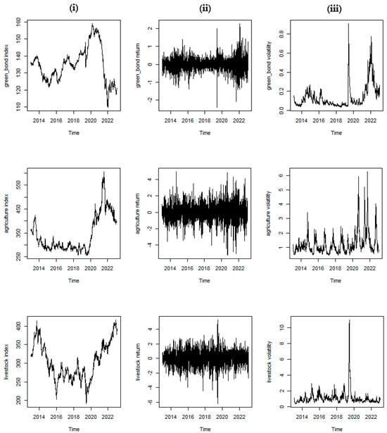
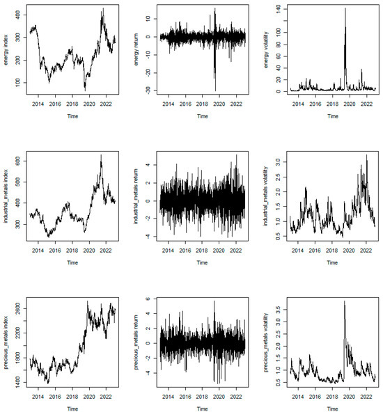
Figure 1.
The data graphs of (i) level, (ii) return, and (iii) volatility series (1 November 2013–24 November 2023).
3.2. MFDCCA Method
In this study, we use MFDCCA to examine the multifractal relationship between green bonds and commodities. The method offered by Zhou [29] is a combination of the DCCA of Podobnik and Stanley [28] and the MFDFA of Kantelhardt et al. [27]. The method allows us to investigate the multifractal behaviour of cross-correlations between bivariate series. It consists of 6 steps described as follows.
Step 1. Let us consider two nonstationary time series whose lengths are equal: and . Construct the profile of the series as follows: calculate the cumulative sums of the series by subtracting arithmetic means ( and ) and cumulatively integrating afterwards.
Step 2. Divide the profiles into nonoverlapping segments with size s as where s is the time scale. Obviously, s will not be the exact multiple of N in most cases. Therefore, we repeat the same segmentation from the starting end of the sequence in order to not discard the remaining observations. In the end, we obtained segments.
Step 3. Find the detrended covariance for each segment g obtained in Step 2.
For segments , we have the following:
For segments , we have the following function:
In Equations (5) and (6), and are obtained from fitting a second-order polynomial to each segment.
In Zhou’s original paper [29], the modulus of the detrended covariance calculation (Equations (5) and (6)) was not considered. Oswiecimka et al. [52] and Kwaipen et al. [53] have pointed out that Zhou’s original method may result in negative cross-covariances, leading to restrictions, for instance, fluctuation functions with complex values and challenges in calculating the generalised Hurst exponents. Various solutions to this problem have been proposed in the literature. For instance, contrary to Zhou’s approach [29], applied studies ([54,55]) propose utilizing the modulus of the cross-covariance function as a solution to the sign issue. This approach has been widely adopted in numerous empirical analyses (e.g., [35,56,57,58,59,60,61]).
While there are alternative methods to handle the sign issue, Oswiecimka et al. [52] introduced a technique called the multifractal cross-correlation method (MFCCA) for this purpose. In our research, we adhere to the prevailing literature and tackle the mentioned issues by applying the modulus to both series in this step, as it signifies the most commonly utilised approach in MFDCCA.
Step 4. The wave (fluctuation) function of order q is calculated by taking the average of local covariance functions of each segment obtained in Step 3.
For , the wave function of order q is obtained as follows:
For , the wave function takes the form:
Step 5. The interaction of wave function and s exhibits the relationship between the two series. If the wave function has a power-law relationship with time scale, then it is concluded that long-range cross-correlations exist between the two series.
Equation (9) is also expressed as follows:
At this point, draw the log–log plot of versus s at each q order. The slope of this regression gives the scaling exponent (or generalised Hurst exponent). If the scaling exponent changes with q order, then we conclude that the cross-correlation between the two series is multifractal. Otherwise, we conclude that the relationship is monofractal. The scaling exponent can be examined to check various multifractal interactions of cross-correlation between the two series. q > 0, shows the relationship in large fluctuation, while q < 0 displays the cross-correlation at small fluctuations. If , the cross-correlation of two pairs is persistent. When , then it is extracted that two series have long-range antipersistent cross-correlation. When , the scaling exponent is the well-known Hurst exponent, and if , it shows that the cross-correlation between the two series is not multifractal; in contrast, it shows a random walk characteristic.
Step 6. In addition to the log–log plot and the scaling exponent, it is required to investigate further evidence of the multifractal relationship between the two series. Zou and Zhang [58] propose to check the Renyi exponent, which is calculated as . If the Renyi exponent nonlinearly increases with q, the cross-correlation of the two series is multifractal. Otherwise, if the Renyi exponent is a linear function of q, then the cross-correlation is single fractal. Another way to check the multifractality of the cross-correlation is to examine the singularity strength and multifractal spectrum . Using Legendre transform, singularity strength and multifractal spectrum are calculated.
The multifractal spectrum is a concave function of the singularity strength in the existence of multifractal cross-correlation. Otherwise, it is said that the series have a single-fractal relationship.
3.3. Cross-Correlation Significance Test
As a preliminary analysis, it is better to check the existence of cross-correlations qualitatively. For this purpose, Podobnik et al. [62] developed the statistic. For two time series and of length N, the cross-correlation function and statistic is obtained as follows:
The test statistic obeys chi-square distribution with m degree of freedom. The cross-correlation is significant between the two series if the statistic exceeds the critical value.
3.4. DCCA Coefficient
The DCCA coefficient of Zebende [63] is used to quantitatively assess bivariate cross-correlations. It is calculated by dividing the fluctuation function of detrended covariance () by the multiplication of the fluctuation function of detrended variances () of individual assets. Here, the fluctuation functions are calculated at .
The DCCA coefficient is bounded . The coefficient is evaluated as follows. For , it shows antipersistent cross-correlation between the two series, while for , it is evidence of the existence of persistent cross-correlation. shows perfectly antipersistent cross-comovement, and if , then the two series exhibit perfect persistent cross-correlation.
4. Findings and Discussion
In this part of the article, we present findings on the multifractal detrended cross-correlation between green bonds and commodities and discuss the results accordingly. For the MFDCCA method, we need to specify some parameters. We choose q such that and set the time scale as . The minimum value of time scale s is set to 10 to avoid incorrect results in polynomial fitting on local trends for [64,65]. For the upper bound on s, we set the maximum value as N/2 to showcase very long-range cross-correlation in the series. Following the recommendation of Ferreira et al. [66] and Saâdaoui [67], we fix the maximum time scale as N/2 to fit robust scaling exponents and highlight long-range interconnectivity between green bonds and commodity markets.
Before proceeding with multifractal analysis, we first test whether the cross-correlations are significant by using Podobnik and Stanley’s [28] test statistic. The test results are given in Figure 2 for return pairs and Figure 3 for volatility pairs, for and at the 95% confidence interval. The test statistics exceed the critical value for all time periods for volatility pairs. For the return series, the test values exceed the critical value for most of the sample period. In general, the results show that both return and volatility pairs of green bonds and commodities have significant cross-correlation.
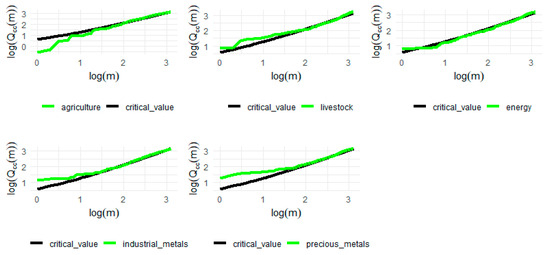
Figure 2.
test results of return series.
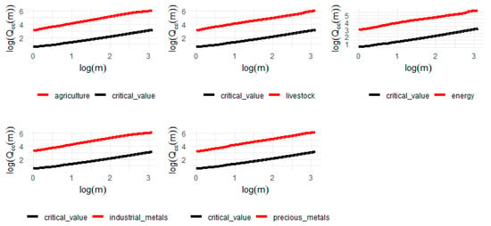
Figure 3.
test results of volatility series.
Proceeding further, Table 2 and Table 3 present coefficients for both return and volatility pairs for . For both the first and second moments, the commodity market and green bonds are highly integrated, and cross-correlations are positive and significant. coefficients are mostly increasing with time scale s, implying that the interconnectedness of green bonds and commodities has long-range interactions. Another observation of the results is that the cross-correlation of volatilities of asset pairs is much stronger than return pairs. It indicates that risk interdependence is much more powerful than returninterdependence for the underlying assets.

Table 2.
DCCA coefficients for return series.

Table 3.
DCCA coefficients for volatility series.
From now on, we direct our focus toward the multifractality of the relationship. In Figure 4, we draw the log–log plot of fluctuation function versus time scale s. As shown in Figure 4, the fluctuation functions of return and volatility pairs are increasing with s, which indicates a power-law relationship in all groups. The result shows the existence of long-range cross-correlation between the green bond market and the commodity market and the existence of multifractality of cross-correlations for both the first and second moments.
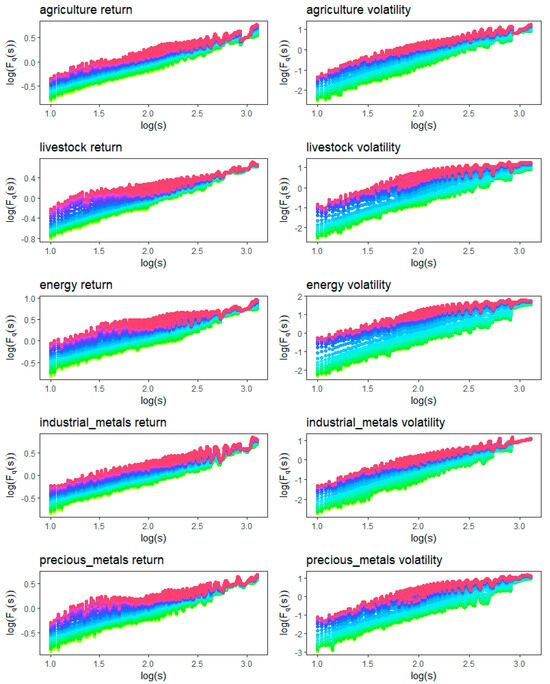
Figure 4.
The log–log plot of fluctuation function vs. time scale s.
The slope of the log–log plots in Figure 4 shows the generalised Hurst exponent (scaling exponent) for various q orders. We obtain the scaling exponent and present the results in Figure 5. We check the Hurst exponent to identify whether the cross-correlations are random walk or they have multifractal structures. The empirical findings show that for all return and volatility pairs, which implies that cross-correlation of the green bond market and the commodity market is not random walk. In addition, the cross-correlation of the markets has multifractal features. Further, we investigate the direction of multifractal cross-correlations with the Hurst exponent at . Both return and volatility pairs have , indicating the long-range persistent cross-correlation. In a general perspective, is the strongest between green bonds and energy/industrial metal markets for the first moment series. On the other hand, it is the strongest among green bonds–industrial metals and green bonds–precious metals pairs at the second moment of the data. Furthermore, we can check how the cross-correlation dynamics occur under small and large fluctuations in the markets. For this aim, we check for small fluctuations and for large fluctuations.
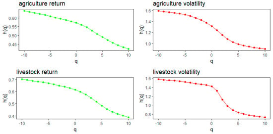
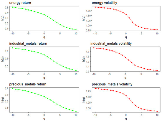
Figure 5.
The generalised Hurst exponents .
Let us discuss the first moment dynamics first. While the market has relatively stable conditions with small fluctuations, all types of commodities exhibit long-range persistent cross-correlations with green bonds. Among them, energies and industrial metals have the highest values, which means that these assets have the strongest persistent cross-correlations. On the other hand, agricultural commodities have the lowest values, which means that the cross-correlations are much lower than others in small fluctuations. But when the market experiences large fluctuations, the commodity market shows antipersistent cross-correlations with green bonds in most of the q orders. Further, precious metals and energies are the assets that have the highest antipersistent cross-correlations.
For volatility pairs, it is observed that commodity market and green bonds always display persistent cross-correlation for both small and large fluctuation conditions. On the other hand, the volatility interconnectedness is much stronger in small fluctuations, whereas it decreases significantly when the market conditions transform through large fluctuations. Energies and metals (precious and industrial) have the strongest persistent cross-correlations in small fluctuations. When the market condition transforms to large fluctuations, it can be seen that agricultural commodities and industrial metals show the most powerful positive comovements with green bonds.
Comparing the results of return and volatility pairs, while return cross-correlations mostly vary over the market conditions, volatilities mostly show similar behaviour, although the power of interconnectedness changes. The return series respond significantly to small and large fluctuations, and the cross-correlation direction changes accordingly. However, the direction of the risk-interdependence of the underlying assets stays the same, although the cross-correlation persistency decreases significantly. It may be due to the fact that while financial risks are highly transmitted between markets and highly interconnected due to the common risk factors, returns are more disposed to be individual and heterogeneous.
In addition to the findings on the power-law relationship of the fluctuation function and time scale, and the generalised Hurst exponent, we provide further evidence on the multifractality of the cross-correlation between green bonds and the commodity market. For this purpose, we present Renyi exponents for various q orders in Figure 6 and multifractal spectrum in Figure 7.
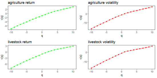
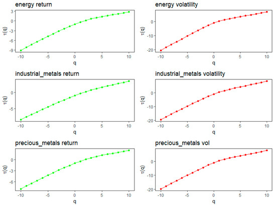
Figure 6.
The Renyi exponents vs. q.
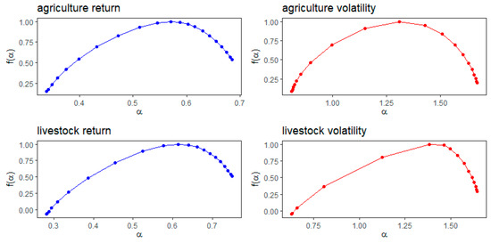
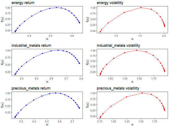
Figure 7.
Singularity strength vs. multifractal spectrum .
The Renyi exponent is supposed to nonlinearly increase with q in the case of multifractality. As can be seen in Figure 6, of the return and volatility series of bivariate pairs is a nonlinear and increasing function of q, which indicates that the cross-correlations of green bonds and the commodity market have multifractal features with complex dynamics. Figure 7 presents the singularity strength and multifractal spectrum for all pairs. The multifractal spectra take concave form for all return and volatility pairs. So, we can further conclude that the cross-correlation between green bonds and commodity markets has multifractal features.
We evaluate the strength of multifractality by calculating the multifractality degree and the width of multifractality . The results are given in Table 4 for return and volatility pairs. For both moments, the multifractality degree and the multifractal spectra width are the largest for energy commodities, indicating the strongest multifractality among all. On the other hand, agricultural commodities display the weakest multifractality with green bonds.

Table 4.
The strength of multifractality analysis.
Further, we examine sources of multifractality in cross-correlations among green bonds and commodities. Multifractality is primarily attributed to two main factors: long memory and fat-tail distributions [68,69,70,71,72]. To evaluate the impact of these sources on the multifractality of cross-correlations, we obtain transformed data and repeat the analysis to compare how the multifractality degree and multifractal spectra width change. For this purpose, we first generate a shuffled series. This process removes long-term memory while preserving the original probability distribution function of the series. We apply 1000*N transpositions on the original series, where N is the length of data, and generate shuffled series. Secondly, we apply the Fourier phase randomisation process and obtain a surrogated series. We conduct discrete Fourier transformation and rotate the transformed series by a random phase angle. Afterwards, we apply inverse Fourier transformation and obtain a surrogated series. This process weakens non-Gaussian distribution while preserving statistical moments and lets us evaluate the contribution of fat-tail distribution on multifractality.
The multifractality degrees and multifractal spectra widths of the transformed data are given in Table 5. After undergoing transformation processes, both return and volatility series exhibit a significant decrease in multifractality strength. This suggests that both long-term memory and heavy-tail distributions contribute to the multifractality of cross-correlations between green bonds and the commodity market.

Table 5.
Sources of multifractality.
For return series, we observe and for livestock, energy, industrial metals, and precious metals, while and is found for agriculture. These findings suggest that heavy tail distributions have the most powerful impact on the multifractality of livestock, energy, industrial metals, and precious metals. On the other hand, the multifractality of cross-correlation of green bonds and agriculture is mainly influenced by long memory in return series.
In the case of volatility pairs, the multifractality degree and the width of multifractal spectra significantly diminish after data transformation. Specifically, for agriculture, livestock, industrial, and precious metals series, it is observed that and . Conversely, for energy volatility series, the sequences and hold true. Thus, while both long memory and fat-tail distributions contribute to the multifractality of volatility series, the dominance of long memory is evident in agriculture, livestock, industrial, and precious metals, whereas fat tails play a more significant role in energy volatility.
5. Conclusions
In recent years, green bonds have become a prominent means of financing environmentally friendly projects, with a growing focus on utilizing commodities, particularly agricultural ones, as underlying assets for these initiatives. The relationship between green bonds and commodities is explored in the literature, with attention to the feasibility, risks, and benefits associated with such connections. Notably, green bonds are suggested to act as a stabilizing force amid commodity price fluctuations, addressing a crucial aspect of risk mitigation. Socially responsible investors are drawn to green bonds as sustainable investment options, and studying their impact on commodities provides insights into the evolving landscape of sustainable finance. While existing research has offered valuable insights using the EMH, there is a notable gap in understanding nonlinear and chaotic dynamics, which the FMH proposes as a more intricate and multifractal perspective on financial markets.
This study employs methods from statistical physics to assess the relationship between green bonds and the commodity market from an econophysics perspective. While a few articles in the existing literature have explored interactions between the two markets, they tend to adhere to the EMH, attempting to explain market behaviour through conventional econometrics and linear approaches. Indeed, econophysicists have repeatedly demonstrated that EMH is insufficient to explain financial markets due to its complex dynamics. We contribute to the literature by exploring the relationship between these two markets, considering their complex structures and nonlinear dynamics. We use MFDCCA and reveal the multifractal cross-correlations between two markets in both return and volatility series.
Our contribution to the literature is threefold. First, we find significant cross-correlations between green bonds and the commodity market. Second, we exhibit that these cross-correlations are positive up to very long lags (e.g., s = 1024). Thirdly, we show that the cross-correlations between two markets are multifractal, both in the first and second moments. Both return and volatility cross-correlations exhibit long-range power-law persistent behaviour. While volatility cross-correlations are always persistent, return series have changing behaviour. When the market is relatively stable with small fluctuations, return cross-correlations of green bonds and commodities exhibit persistent behaviour. On the other hand, when the market experiences large fluctuations, the cross-correlations of return series become antipersistent. In addition, our analysis of the sources of multifractality indicates that long memory and heavy-tail distributions contribute to the multifractality of cross-correlations.
For portfolio implications, we recommend using commodities to hedge the risk in green bonds and vice versa, as these assets exhibit high and persistent cross-correlation at second moments. Investors in these markets can adopt inverse positions to mitigate volatility in their initial holdings. From a general perspective, the green bonds–precious metals pair has the lowest persistent cross-correlation. Consequently, these two assets can be combined for portfolio diversification in long positions. For short traders, the green bond–industrial metal pairs can be considered as two inverse positions due to their high and persistent return cross-correlations. Additionally, we provide two specific examples for both extreme cases. However, investors can also consider other commodities based on their risk preferences.
The previous literature highlights the portfolio diversification and hedging benefits of green bonds for the commodity market. Nguyen et al. [12] utilised the wavelet correlation method and demonstrated that green bonds perform very well in commodity portfolios. Similarly, Naeem et al. [11] and Arif et al. [10] supported the findings of Nguyen et al. [12] by using the cross-quantilogram method. Furthermore, Naeem et al. [12] and Tsagkanos et al. [13] provided similar results on time–frequency connectedness and copula–VaR models. In this study, we support the previous findings with some crucial facts. In contrast to the previous studies, we reject the EMH and show that the interconnectivity between green bonds and commodities is multifractal. Also, while the previous literature offers one-dimensional basic portfolio and hedging activities for green bonds and commodities, we show that due to the complex dynamics in the market, these suggestions cannot be straightforward. This study illustrates how portfolio applications and hedging activities should be realised under multifractal characteristics and various fluctuations in the market.
Future studies may delve deeper into exploring the multifractality of green bonds in relation to other financial assets. Another potential avenue for research could involve examining multifractal dynamics through time-varying analysis. Our study primarily focuses on a full-sample analysis; however, it is essential to acknowledge that complex dynamics may undergo variations over time. Investigating these dynamics across different time periods could provide valuable insights into the evolving nature of the multifractal characteristics associated with green bonds and their interactions with other financial instruments.
Author Contributions
Conceptualisation, T.A., S.G. and A.B.S.; methodology, T.A.; software, T.A.; validation, T.A., S.G. and A.B.S.; formal analysis, T.A., S.G. and A.B.S.; investigation, T.A. and A.B.S.; writing—original draft preparation, T.A., S.G. and A.B.S.; writing—review and editing, T.A., S.G. and A.B.S. All authors have read and agreed to the published version of the manuscript.
Funding
This research received no external funding.
Data Availability Statement
Publicly available datasets were used in this study. The data can be found on S&P’s website: https://www.spglobal.com/spdji/en/ (accessed on 8 January 2024).
Conflicts of Interest
The authors declare no conflicts of interest.
References
- Zhang, D.; Zhang, Z.; Managi, S. A Bibliometric Analysis on Green Finance: Current Status, Development, and Future Directions. Finance Res. Lett. 2019, 29, 425–430. [Google Scholar] [CrossRef]
- Reboredo, J.C.; Ugolini, A. Price Connectedness between Green Bond and Financial Markets. Econ. Model. 2020, 88, 25–38. [Google Scholar] [CrossRef]
- Climate Bond Initiative Sustainable Debt Global State of the Market Report 2022. 2023. Available online: https://www.climatebonds.net/resources/reports/global-state-market-report-2022 (accessed on 13 February 2024).
- MacAskill, S.; Roca, E.; Liu, B.; Stewart, R.A.; Sahin, O. Is There a Green Premium in the Green Bond Market? Systematic Literature Review Revealing Premium Determinants. J. Clean. Prod. 2021, 280, 124491. [Google Scholar] [CrossRef]
- Banga, J. The Green Bond Market: A Potential Source of Climate Finance for Developing Countries. J. Sustain. Finance Investig. 2019, 9, 17–32. [Google Scholar] [CrossRef]
- Basak, S.; Pavlova, A. A Model of Financialization of Commodities. J. Finance 2016, 71, 1511–1556. [Google Scholar] [CrossRef]
- Acikgoz, T.; Alp, O.S.; Alkan, N.B. Dynamics of a Newly Established Agricultural Commodities Market: Financialization, Hedging and Portfolio Diversification in Turkey. Ann. Finance Econ. 2023, 18, 2350005. [Google Scholar] [CrossRef]
- Tang, K.; Xiong, W. Index Investment and the Financialization of Commodities. Finance Anal. J. 2012, 68, 54–74. [Google Scholar] [CrossRef]
- Nguyen, T.T.H.; Naeem, M.A.; Balli, F.; Balli, H.O.; Vo, X.V. Time-Frequency Comovement among Green Bonds, Stocks, Commodities, Clean Energy, and Conventional Bonds. Finance Res. Lett. 2021, 40, 101739. [Google Scholar] [CrossRef]
- Arif, M.; Naeem, M.A.; Farid, S.; Nepal, R.; Jamasb, T. Diversifier or More? Hedge and Safe Haven Properties of Green Bonds during COVID-19. Energy Policy 2022, 168, 113102. [Google Scholar] [CrossRef] [PubMed]
- Naeem, M.A.; Adekoya, O.B.; Oliyide, J.A. Asymmetric Spillovers between Green Bonds and Commodities. J. Clean. Prod. 2021, 314, 128100. [Google Scholar] [CrossRef]
- Naeem, M.A.; Nguyen, T.T.H.; Nepal, R.; Ngo, Q.-T.; Taghizadeh–Hesary, F. Asymmetric Relationship between Green Bonds and Commodities: Evidence from Extreme Quantile Approach. Finance Res. Lett. 2021, 43, 101983. [Google Scholar] [CrossRef]
- Tsagkanos, A.; Sharma, A.; Ghosh, B. Green Bonds and Commodities: A New Asymmetric Sustainable Relationship. Sustainability 2022, 14, 6852. [Google Scholar] [CrossRef]
- Carter, C.A.; Rausser, G.C.; Smith, A. Commodity Booms and Busts. Annu. Rev. Resour. Econ. 2011, 3, 87–118. [Google Scholar] [CrossRef]
- Acar, S.; Yeldan, E. Handbook of Green Economics; Academic Press: Cambridge, MA, USA, 2019; ISBN 0128166444. [Google Scholar]
- Reboredo, J.C. Green Bond and Financial Markets: Co-Movement, Diversification and Price Spillover Effects. Energy Econ. 2018, 74, 38–50. [Google Scholar] [CrossRef]
- Reboredo, J.C.; Ugolini, A.; Aiube, F.A.L. Network Connectedness of Green Bonds and Asset Classes. Energy Econ. 2020, 86, 104629. [Google Scholar] [CrossRef]
- Khamis, M.; Aassouli, D. The Eligibility of Green Bonds as Safe Haven Assets: A Systematic Review. Sustainability 2023, 15, 6841. [Google Scholar] [CrossRef]
- Research Department, International Monetary Fund. World Economic Outlook, October 2020: A Long and Difficult Ascent; International Monetary Fund: Washington, DC, USA, 2020; ISBN 9781513556055. [Google Scholar]
- Mezghani, T.; Ben Hamadou, F.; Boujelbène-Abbes, M. Network Connectedness and Portfolio Hedging of Green Bonds, Stock Markets and Commodities. Int. J. Emerg. Mark. 2023; ahead-of-print. [Google Scholar] [CrossRef]
- Fama, E.F. Efficient Capital Markets: A Review of Theory and Empirical Work. J. Finance 1970, 25, 383–417. [Google Scholar] [CrossRef]
- Peters, E.E. Fractal Market Analysis: Applying Chaos Theory to Investment and Economics; John Wiley & Sons: Hoboken, NJ, USA, 1994; Volume 24. [Google Scholar]
- Mandelbrot, B. The Variation of Certain Speculative Prices. J. Bus. 1963, 36, 394–419. [Google Scholar] [CrossRef]
- Mandelbrot, B.B. A Multifractal Walk down Wall Street. Sci. Am. 1999, 280, 70–73. [Google Scholar] [CrossRef]
- Mandelbrot, B.B.; Van Ness, J.W. Fractional Brownian Motions, Fractional Noises and Applications. SIAM Rev. 1968, 10, 422–437. [Google Scholar] [CrossRef]
- Peng, C.-K.; Buldyrev, S.V.; Havlin, S.; Simons, M.; Stanley, H.E.; Goldberger, A.L. Mosaic Organization of DNA Nucleotides. Phys. Rev. E 1994, 49, 1685–1689. [Google Scholar] [CrossRef]
- Kantelhardt, J.W.; Zschiegner, S.A.; Koscielny-Bunde, E.; Havlin, S.; Bunde, A.; Stanley, H.E. Multifractal Detrended Fluctuation Analysis of Nonstationary Time Series. Phys. A Stat. Mech. Its Appl. 2002, 316, 87–114. [Google Scholar] [CrossRef]
- Podobnik, B.; Stanley, H.E. Detrended Cross-Correlation Analysis: A New Method for Analyzing Two Nonstationary Time Series. Phys. Rev. Lett. 2008, 100, 84102. [Google Scholar] [CrossRef] [PubMed]
- Zhou, W.-X. Multifractal Detrended Cross-Correlation Analysis for Two Nonstationary Signals. Phys. Rev. E 2008, 77, 66211. [Google Scholar] [CrossRef] [PubMed]
- Pan, Y.; Hou, L.; Pan, X. Interplay between Stock Trading Volume, Policy, and Investor Sentiment: A Multifractal Approach. Phys. A Stat. Mech. Its Appl. 2022, 603, 127706. [Google Scholar] [CrossRef]
- Li, X.; Su, F. The Dynamic Effects of COVID-19 and the March 2020 Crash on the Multifractality of NASDAQ Insurance Stock Markets. Fractal Fract. 2023, 7, 91. [Google Scholar] [CrossRef]
- Fernandes, L.H.S.; Silva, J.W.L.; Quintino, D.D.; De Araujo, F.H.A.; Tabak, B.M. Multifractal Cross-Correlations Risk among WTI and Financial Assets. Fractals 2022, 30, 2250191. [Google Scholar] [CrossRef]
- Shao, Y.-H.; Liu, Y.-L.; Yang, Y.-H. The Short-Term Effect of COVID-19 Pandemic on China’s Crude Oil Futures Market: A Study Based on Multifractal Analysis. Fluct. Noise Lett. 2022, 22, 2340001. [Google Scholar] [CrossRef]
- Aslam, F.; Zil-E-Huma; Bibi, R.; Ferreira, P. The Nexus Between Twitter-Based Uncertainty and Cryptocurrencies: A Multifractal Analysis. Fractals 2023, 31, 2350027. [Google Scholar] [CrossRef]
- Ruan, Q.; Meng, L.; Lv, D. Effect of Introducing Bitcoin Futures on the Underlying Bitcoin Market Efficiency: A Multifractal Analysis. Chaos Solitons Fractals 2021, 153, 111576. [Google Scholar] [CrossRef]
- Ma, J.; Wang, T.; Zhao, R. Quantifying Cross-Correlations between Economic Policy Uncertainty and Bitcoin Market: Evidence from Multifractal Analysis. Discrete Dyn. Nat. Soc. 2022, 2022, 1072836. [Google Scholar] [CrossRef]
- Ali, H.; Aslam, F.; Ferreira, P. Modeling Dynamic Multifractal Efficiency of US Electricity Market. Energies 2021, 14, 6145. [Google Scholar] [CrossRef]
- Fu, Z.; Niu, H.; Wang, W. Market Efficiency and Cross-Correlations of Chinese New Energy Market with Other Assets: Evidence from Multifractality Analysis. Comput. Econ. 2023, 62, 1287–1311. [Google Scholar] [CrossRef] [PubMed]
- Yang, W.; Ruan, Q.; Yin, L. Non-Linear Impact of Chinese Treasury Bond Futures on the Information Content of IRS. Fluct. Noise Lett. 2021, 20, 2150051. [Google Scholar] [CrossRef]
- Wang, J.; Jiang, W.; Yan, Y.; Shao, W.; Wu, X.; Hua, Z. Exploring the Asymmetric Multifractal Characteristics of Price–Volume Cross-Correlation in the Chinese Rebar Futures Market Based on MF-ADCCA. Fluct. Noise Lett. 2023, 22, 2350029. [Google Scholar] [CrossRef]
- Fernandes, L.H.S.; Silva, J.W.L.; de Araujo, F.H.A.; Tabak, B.M. Multifractal Cross-Correlations between Green Bonds and Financial Assets. Finance Res. Lett. 2023, 53, 103603. [Google Scholar] [CrossRef]
- Shishlov, I.; Morel, R.; Cochran, I. Beyond Transparency: Unlocking the Full Potential of Grene Bonds. Inst. Clim. Change 2016, 2, 1–28. [Google Scholar]
- Flaherty, M.; Gevorkyan, A.; Radpour, S.; Semmler, W. Financing Climate Policies through Climate Bonds—A Three Stage Model and Empirics. Res. Int. Bus. Finance 2017, 42, 468–479. [Google Scholar] [CrossRef]
- Flammer, C. Corporate Green Bonds. J. Finance Econ. 2021, 142, 499–516. [Google Scholar] [CrossRef]
- Guo, D.; Zhou, P. Green Bonds as Hedging Assets before and after COVID: A Comparative Study between the US and China. Energy Econ. 2021, 104, 105696. [Google Scholar] [CrossRef]
- Jiang, Y.; Wang, J.; Ao, Z.; Wang, Y. The Relationship between Green Bonds and Conventional Financial Markets: Evidence from Quantile-on-Quantile and Quantile Coherence Approaches. Econ. Model. 2022, 116, 106038. [Google Scholar] [CrossRef]
- Han, Y.; Li, J. Should Investors Include Green Bonds in Their Portfolios? Evidence for the USA and Europe. Int. Rev. Finance Anal. 2022, 80, 101998. [Google Scholar] [CrossRef]
- Ren, B.; Lucey, B.; Luo, Q. An Examination of Green Bonds as a Hedge and Safe Haven for International Equity Markets. Glob. Finance J. 2023, 58, 100894. [Google Scholar] [CrossRef]
- Tang, D.Y.; Zhang, Y. Do Shareholders Benefit from Green Bonds? J. Corp. Finance 2020, 61, 101427. [Google Scholar] [CrossRef]
- Pham, L. Is It Risky to Go Green? A Volatility Analysis of the Green Bond Market. J. Sustain. Finance Investig. 2016, 6, 263–291. [Google Scholar] [CrossRef]
- Gao, Y.; Li, Y.; Wang, Y. Risk Spillover and Network Connectedness Analysis of China’s Green Bond and Financial Markets: Evidence from Financial Events of 2015–2020. N. Am. J. Econ. Finance 2021, 57, 101386. [Google Scholar] [CrossRef]
- Oświȩcimka, P.; Drożdż, S.; Forczek, M.; Jadach, S.; Kwapień, J. Detrended Cross-Correlation Analysis Consistently Extended to Multifractality. Phys. Rev. E 2014, 89, 23305. [Google Scholar] [CrossRef]
- Kwapień, J.; Oświęcimka, P.; Drożdż, S. Detrended Fluctuation Analysis Made Flexible to Detect Range of Cross-Correlated Fluctuations. Phys. Rev. E 2015, 92, 52815. [Google Scholar] [CrossRef]
- He, L.-Y.; Chen, S.-P. Nonlinear Bivariate Dependency of Price–Volume Relationships in Agricultural Commodity Futures Markets: A Perspective from Multifractal Detrended Cross-Correlation Analysis. Phys. A Stat. Mech. Its Appl. 2011, 390, 297–308. [Google Scholar] [CrossRef]
- Li, Z.; Lu, X. Cross-Correlations between Agricultural Commodity Futures Markets in the US and China. Phys. A Stat. Mech. Its Appl. 2012, 391, 3930–3941. [Google Scholar] [CrossRef]
- Cai, Y.; Lu, X.; Ren, Y.; Qu, L. Exploring the Dynamic Relationship between Crude Oil Price and Implied Volatility Indices: A MF-DCCA Approach. Phys. A Stat. Mech. Its Appl. 2019, 536, 120973. [Google Scholar] [CrossRef]
- Charutha, S.; Gopal Krishna, M.; Manimaran, P. Multifractal Analysis of Indian Public Sector Enterprises. Phys. A Stat. Mech. Its Appl. 2020, 557, 124881. [Google Scholar] [CrossRef]
- Zou, S.; Zhang, T. Multifractal Detrended Cross-Correlation Analysis of the Relation between Price and Volume in European Carbon Futures Markets. Phys. A Stat. Mech. Its Appl. 2020, 537, 122310. [Google Scholar] [CrossRef]
- Fernandes, L.H.S.; Silva, J.W.L.; de Araujo, F.H.A.; Ferreira, P.; Aslam, F.; Tabak, B.M. Interplay Multifractal Dynamics among Metal Commodities and US-EPU. Phys. A Stat. Mech. Its Appl. 2022, 606, 128126. [Google Scholar] [CrossRef]
- Telli, Ş.; Chen, H. Multifractal Behavior Relationship between Crypto Markets and Wikipedia-Reddit Online Platforms. Chaos Solitons Fractals 2021, 152, 111331. [Google Scholar] [CrossRef]
- Zhuang, X.; Wei, Y.; Zhang, B. Multifractal Detrended Cross-Correlation Analysis of Carbon and Crude Oil Markets. Phys. A Stat. Mech. Its Appl. 2014, 399, 113–125. [Google Scholar] [CrossRef]
- Podobnik, B.; Jiang, Z.-Q.; Zhou, W.-X.; Stanley, H.E. Statistical Tests for Power-Law Cross-Correlated Processes. Phys. Rev. E 2011, 84, 66118. [Google Scholar] [CrossRef] [PubMed]
- Zebende, G.F. DCCA Cross-Correlation Coefficient: Quantifying Level of Cross-Correlation. Phys. A Stat. Mech. Its Appl. 2011, 390, 614–618. [Google Scholar] [CrossRef]
- Zhang, S.; Guo, Y.; Cheng, H.; Zhang, H. Cross-Correlations between Price and Volume in China’s Crude Oil Futures Market: A Study Based on Multifractal Approaches. Chaos Solitons Fractals 2021, 144, 110642. [Google Scholar] [CrossRef]
- Lin, Y.; Wang, R.; Gong, X.; Jia, G. Cross-Correlation and Forecast Impact of Public Attention on USD/CNY Exchange Rate: Evidence from Baidu Index. Phys. A Stat. Mech. Its Appl. 2022, 604, 127686. [Google Scholar] [CrossRef]
- Ferreira, P.; Dionísio, A.; Movahed, S.M.S. Assessment of 48 Stock Markets Using Adaptive Multifractal Approach. Phys. A Stat. Mech. Its Appl. 2017, 486, 730–750. [Google Scholar] [CrossRef]
- Saâdaoui, F. Testing for Multifractality of Islamic Stock Markets. Phys. A Stat. Mech. Its Appl. 2018, 496, 263–273. [Google Scholar] [CrossRef]
- Matia, K.; Ashkenazy, Y.; Stanley, H.E. Multifractal Properties of Price Fluctuations of Stocks and Commodities. Europhys. Lett. 2003, 61, 422. [Google Scholar] [CrossRef]
- Sadegh Movahed, M.; Jafari, G.R.; Ghasemi, F.; Rahvar, S.; Reza Rahimi Tabar, M. Multifractal Detrended Fluctuation Analysis of Sunspot Time Series. J. Stat. Mech. Theory Exp. 2006, 2006, P02003. [Google Scholar] [CrossRef]
- Zhou, W.-X. The Components of Empirical Multifractality in Financial Returns. Europhys. Lett. 2009, 88, 28004. [Google Scholar] [CrossRef]
- Ruan, Q.; Jiang, W.; Ma, G. Cross-Correlations between Price and Volume in Chinese Gold Markets. Phys. A Stat. Mech. Its Appl. 2016, 451, 10–22. [Google Scholar] [CrossRef]
- Shen, N.; Chen, J.Y. Multifractal Analysis of the Impact of COVID-19 on NASDAQ, CIOPI, and WTI Crude Oil Market. Fluct. Noise Lett. 2022, 21, 2250041. [Google Scholar] [CrossRef]
Disclaimer/Publisher’s Note: The statements, opinions and data contained in all publications are solely those of the individual author(s) and contributor(s) and not of MDPI and/or the editor(s). MDPI and/or the editor(s) disclaim responsibility for any injury to people or property resulting from any ideas, methods, instructions or products referred to in the content. |
© 2024 by the authors. Licensee MDPI, Basel, Switzerland. This article is an open access article distributed under the terms and conditions of the Creative Commons Attribution (CC BY) license (https://creativecommons.org/licenses/by/4.0/).