Fast Linear Canonical Transform for Nonequispaced Data

Abstract

The investigations of the discrete and fast linear canonical transform (LCT) are becoming one of the hottest research topics in modern signal processing and optics. Among them, the fast calculation of LCT for non-uniform data is one of key problems. Focus on this problem, a new fast algorithm of the LCT has been proposed in this paper firstly by interpolation and approximation theory. The proposed algorithms can calculate quickly the LCT of the data, whether the input or output data is uniform. Secondly, the complexity and precision of derived algorithms have been analyzed for different situations. Finally, the experimental results are presented to verify the correctness of the obtained results.

1. Introduction

Linear canonical transform which is generated by second-order differential operators, is a four-parameter class of linear integral transform [1,2],

$$F^A(u)=\left\{\begin{array}{cc}{\int }_{-\infty }^{\infty }x(t)K_A(t,u)dt,\hfill & b\ne 0\hfill \\ \sqrt{(}d)e^{i\frac{cd{u}^2}{2}}x(du),\hfill & b=0\hfill \end{array}\right.$$

where

$$K_A(t,u)=\frac{1}{i2\pi b}{e}^{i\frac{a}{2b}{t}^2-i\frac{tu}{b}+i\frac{d}{2b}{u}^2}$$

$A=[a,b;c,d], ad-bc=1, F^A(u)$ is LCT of the function $x(t)$. The LCT integral kernels are Green functions of quadratic Hamiltonians that can be found in [3]. The research on LCT was first proposed by Collins (1970) and Moshinsky (1971) [1,2]. It includes many special cases, such as, the Fourier transform (FT), the fractional Fourier transform (FRFT), the Fresnel transform, the Lorentz transform and scaling transform. The class of LCTs are important in signal processing [4,5], computational and applied mathematics [6,7], optics [8] and quantum mechanics [9]. Significant applications of LCT in signal processing include radar system analysis, filter design, pattern recognition, image watermarking and so on [10,11]. Basic theories of LCT have been developed that include convolution theorems, sampling theorems, and uncertainty principles [12,13,14]. The numerical approximation of the LCT is of importance in modeling first-order optical systems and many signal processing applications. Therefore, the discrete and fast algorithms of the LCT are one of the most important issues in practical applications.

After the continuous LCT has been introduced, therefore, the definition and fast implementation of the discrete linear canonical transform (DLCT) have been widely considered by many researchers [15,16,17,18,19,20,21,22,23,24,25,26,27,28]. The existing algorithms can be divided into the following categories. The one is the operator decomposition type, which decomposes an arbitrary LCT operator into its special cases that have a fast algorithm [17,18,29]. The second is the eigenvector decomposition type, which computes the LCT of a function by using the eigenfunctions of the LCT [24,27]. The third is split basis algorithm, which decomposes the discrete transform matrix of LCT into smaller matrices iteratively [20,23]. All these algorithms can effectively and rapidly calculate the entire spectrum in the LCT domain. In recent years, the new LCT algorithms have been proposed, which can realize local spectrum analysis of signals [30,31,32]. In addition to the above-mentioned algorithms, various other fast algorithms have been proposed in [33,34,35,36,37,38,39]. These research results provide a good basis for the further development of the DLCT toward meeting the requirements of practical applications. Many aspects of the fast methods of the DLCT still need to be studied. To the best of our knowledge, the existing discrete algorithms are required that both input and output data are uniform sampling. However, for certain applications, the input or output data is nonuniform. In these cases, the fast DLCT will be lost.

For overcome the aforementioned problems, in this paper, we present a set of fast algorithms for computing nonuniform DLCT, namely,

$$f(t_n)=\frac{1}{\sqrt{-i2\pi b}}\sum _{m=0}^{N-1}{\alpha }_m{e}^{-i\frac{a}{2b}{t}_n^2+i\frac{u_m{t}_n}{b}-i\frac{d}{2b}{u}_m^2}$$

(1)

where $n=0,1,\cdots N$, $f(t_n)\in \mathbf{C}$, ${\alpha }_m\in \mathbf{C}$, $t_n\in [-b\pi ,b\pi ]$, and $u_m\in [-N/2,N/2-1]$. According to the sampling of the $t_n$ and $u_m$, we will operate under the following assumptions

• Uniform samples and non integer frequencies: In Equation (1) the samples are equispaced, i.e., $t_j=j2\pi \left|b\right|/N$, and the frequencies $u_0,\cdots ,u_{N-1}$ are non integer. This corresponds to evaluating a generalized linear canonical series at equispaced points.
• Nonuniform samples and integer frequencies: In Equation (1), $t_0,\cdots ,t_{N-1}$ are nonequispaced points in $[-b\pi ,b\pi ]$ and the frequencies $u_0,\cdots ,u_{N-1}$ are integers.
• Nonuniform samples and non-integer frequencies: In Equation (1), $t_0,\cdots ,t_{N-1}$ are nonequispaced points in $[-b\pi ,b\pi ]$ and the frequencies $u_0,\cdots ,u_{N-1}$ are non-integers. This is the fully nonuniform transform and corresponds to evaluating a generalize linear canonical series at nonequispaced points.

To develop various nonuniform fast LCT(NFLCT) for above issues, one has to exploit a nonzero working precision of $0<ϵ<1$ and makes careful approximations. The approximation properties of the various approaches may be obtained by considering how they perform on the linear canonical modes.

The rest of the paper is organized as follows: In Section 2, a brief review of the related preliminaries is presented which are used in the design of the algorithms. The Section 3 is main results of this paper. In this section, we give an exact statement of the problem and introduce some notation that is used. The algorithms are derived. Some numerical examples are presented in Section 4 to illustrate the preference of the schemes. Finally, conclusions are drawn in Section 5.

2. Preliminary

The linear canonical series (LCS) is a generalized form of Fourier series (FS), which can reveal the mixed time and frequency components of signals. The basis function of LCS is defined as [40]

$${\phi }_{A,n}(t)=\sqrt{\frac{i}{T}}{e}^{-i\frac{a}{2b}{t}^2-i\frac{d}{2b}{(n2\pi b/T)}^2+i\frac{t}{b}(n2\pi b/T)}$$

(2)

where $n=-\infty ,\cdots ,-1,0,1,\cdots ,+\infty$. Thus, $\left\{\cdots ,{\phi }_{A,-1}(t),{\phi }_{A,0}(t),{\phi }_{A,1}(t),\cdots \right\}$ construct an orthonormal basis. It can be observed that every basis function is a chirp function with chirp rate $-a/b$, which is an aperiodic function. Therefore, the LCS is only applicable to finite-length function. The LCS expansion of the finite-length function $x(t)$ can be written as

$$x(t)=\sum _{n=-\infty }^{\infty }{C}_{A,n}{\phi }_{A,n}(t)=\sum _{n=-\infty }^{\infty }{C}_{A,n}\sqrt{\frac{i}{T}}{e}^{-i\frac{a}{2b}{t}^2-i\frac{d}{2b}{(n2\pi b/T)}^2+i\frac{t}{b}(n2\pi b/T)}$$

(3)

$$C_{A,n}=\sqrt{\frac{-i}{T}}{\int }_{-T/2}^{T/2}x(t)e^{i\frac{a}{2b}{t}^2+i\frac{d}{2b}{(n2\pi b/T)}^2-i\frac{t}{b}(n2\pi b/T)}\mathrm{d}t$$

(4)

where $t\in [-T/2,T/2]$ and $C_{A,n}$ are called LCS expansion coefficients with the parameter matrix A.The LCS expansion coefficients are computed by the inner product of the function and chirp basis function. The relationship between LCS and LCT is that the LCS expansion coefficients are the sampled values of LCT, by

$$C_{A,n}=\sqrt{\frac{2\pi b}{T}}{F}^A\left[x(t)\right](n\frac{2\pi b}{T})$$

(5)

The well-known FS is just a special case of LCS for the parameter matrix $A=[0,1;-1,0]$. In addition, we also presented some well results to be used in the remainder of the paper [41].

Lemma 1.

For any real $\alpha >0$ and complex z,

$${\int }_{-\infty }^{\infty }{e}^{-\alpha t^2}{e}^{zt}dt=\sqrt{\frac{\pi }{\alpha }}{e}^{z^2/4\alpha }$$

(6)

Lemma 2.

For any real $\alpha >0$ and $r>0$,

$${\int }_r^{\infty }{e}^{-\alpha t^2}dt<\frac{e^{-\alpha r^2}}{2\alpha r}$$

(7)

In the next section, the main results will be derived based on above facts.

3. Main Results

3.1. Exact Statement of the Problem and Information Description of the Algorithm

3.1.1. Exact Statement of the Problem

In the reminder of this paper, we will operate under the following assumptions:

1.

$u=\left\{u_0,u_1,\cdots ,u_{N-1}\right\}$ and $t=\left\{t_0,t_1,\cdots ,t_{N-1}\right\}$ are finite sequences of real numbers.

2.

$u_m\in [-N/2,N/2-1]$ for $m=0,1,\cdots ,N-1$.

3.

$t_j\in [-b\pi ,b\pi ]$ for $j=0,1,\cdots ,N-1$.

4.

$\mathsf{\alpha }=\left\{{\alpha }_0,\cdots ,{\alpha }_{N-1}\right\}$, $\mathbf{f}=\left\{f_{-N/2},\cdots ,f_{N/2-1}\right\}$, $\mathsf{\beta }=\left\{{\beta }_{-N/2},\cdots ,{\beta }_{N/2-1}\right\}$,

$\mathbf{g}=\left\{g_0,g_1,\cdots ,g_{N-1}\right\}$, $\mathsf{\gamma }=\left\{{\gamma }_0,\cdots ,{\gamma }_{N-1}\right\}$ and $\left\{h_0,h_1,\cdots ,h_{N-1}\right\}$ are finite sequences of complex numbers.

We will consider the problems of applying and inverting the LCT and its transpose. We are interested in the transformations $F,G$: $C^N\to C^N$ and their inverse defined by  formulate

$$f_j=F{(\mathsf{\alpha })}_j=\sum _{k=0}^{N-1}{\alpha }_k{e}^{-i\frac{a}{2b}{(\frac{2b\pi j}{N})}^2+i\frac{u_k}{b}\frac{2\pi j}{N}-i\frac{d}{2b}{u}_k^2}$$

(8)

for $j=-N/2,\cdots ,N/2-1$, and

$$g_j=G{(\mathbf{g})}_j=\sum _{k=-N/2}^{N/2-1}{\beta }_k{e}^{-i\frac{a}{2b}{t}_j^2+i\frac{k{t}_j}{b}-i\frac{d}{2b}{k}^2}$$

(9)

For $j=0,1,\cdots ,N-1$, we will also consider the more general transformation $H:C^N\to C^N$ defined by the formula

$$h_j=H{(\mathsf{\gamma })}_j=\sum _{k=0}^{N-1}{\gamma }_k{e}^{-i\frac{a}{2b}{t}_j^2+i\frac{u_k{t}_j}{b}-i\frac{d}{2b}{u}_k^2}$$

(10)

More formally, we consider that give $\mathsf{\alpha }$, $\mathsf{\beta }$, $\mathsf{\gamma }$ to find $F^A(\mathsf{\alpha })$, $G^A(\mathsf{\beta })$, $H^A(\mathsf{\gamma })$ respectively.

3.1.2. Information Description of the Algorithm

In this section, we give information outlines of algorithms for above problems. The algorithms are based on the following principal steps. Any function $e^{-ia/(2b)t^2+i\beta t/b-id/(2b){\beta }^2}$ can be accurately represented on any finite interval on the real line using a small number of terms of the $e^{\alpha t^2}{e}^{-ia/(2b)t^2+ikt/b-id/(2b)k^2}$ and this number of terms of q is independent of the value $\beta$. For the efficient calculation Equations (8)–(10), the following two ways will be used,

• to approximate each $e^{-ia{t}^2/2b+i{u}_{m}t/b-id{u}_m^2/2b}$ in term of a q-term LCS;
• to approximate the value of a LCS at each $t_n$ in terms of values at the nearest q uniformly-spaced nodes.

The interpolation between equispaced and nonequispaced sets of points can thus be performed in $O(Nq)$ operations.

3.2. Derivation of Algorithms

3.2.1. Relevant Facts from Approximation Theory

The principal tool of this paper is a detailed analysis of the LCS of functions $\varphi :[-b\pi ,b\pi ]\to \mathbf{C}$ given by the formula

$$\varphi (t)=e^{-\alpha t^2}{e}^{-i\frac{a}{2b}{t}^2+i\frac{\beta t}{b}-i\frac{d}{2b}{\beta }^2}$$

(11)

where $\alpha >1/2$ and $\beta$ are real numbers. The lemmas and theorems are presented in the  following.

Theorem 1.

The functions $\varphi (t)=e^{-\alpha t^2}{e}^{-i\frac{a}{2b}{t}^2+i\frac{\beta t}{b}-i\frac{d}{2b}{\beta }^2}$, $t\in (-b\pi ,b\pi )$ can be approximated by LCS, the error of the approximation can be obtained by the following inequality

$$\begin{array}{cc}\hfill & \left|\varphi (t)-\sum _{k=-\infty }^{\infty }{\rho }_{A,k}\sqrt{\frac{i}{2b\pi }}{e}^{-i\frac{a}{2b}{t}^2+i\frac{kt}{b}-i\frac{d}{2b}{k}^2}\right|\hfill \\ \hfill & <e^{-\alpha b^2{\pi }^2}\left[(1+\frac{1}{{\pi }^2{b}^2})(\frac{8\alpha (1+4b)}{9}+2b\pi +2)+1\right]\hfill \end{array}$$

(12)

where $k=-\infty ,\cdots ,\infty$

$${\rho }_{A,k}=\sqrt{\frac{-i}{2b\pi }}{e}^{i\frac{d}{2b}(k^2-{\beta }^2)}\sqrt{\frac{\pi }{\alpha }}{e}^{-\frac{{(\beta -k)}^2}{4b^2\alpha }}$$

(13)

$a,b,c,d$ are linear canonical parameters, $\alpha >1/2$ and β are any real, $q\ge 4\alpha b^2\pi$ is even integer.

Proof. 

The kth LCS coefficient for $\varphi (t)$ is denoted by ${\sigma }_{A,k}$,

$$\varphi (t)=\sqrt{\frac{i}{2b\pi }}\sum _{k=-\infty }^{\infty }{\sigma }_{A,k}{e}^{-i\frac{a}{2b}{t}^2+i\frac{kt}{b}-i\frac{d}{2b}{k}^2}$$

(14)

where $t\in (-b\pi ,b\pi )$,

$$\begin{array}{c}\hfill {\sigma }_{A,k}=\sqrt{\frac{-i}{2b\pi }}{\int }_{-b\pi }^{b\pi }{e}^{i\frac{a}{2b}{t}^2-i\frac{kt}{b}+i\frac{d}{2b}{k}^2}\varphi (t)dt\end{array}$$

(15)

For any real $\alpha >0$ and complex z, we have the following equality

$${\int }_{-\infty }^{\infty }{e}^{-\alpha t^2}{e}^{zt}dt=\sqrt{\frac{\pi }{\alpha }}{e}^{z^2/4\alpha }$$

(16)

thus

$$\begin{array}{cc}\hfill {\sigma }_{A,k}& =\sqrt{\frac{-i}{2b\pi }}{\int }_{-b\pi }^{b\pi }{e}^{-\alpha t^2}{e}^{-i\frac{a}{2b}{t}^2+i\frac{\beta t}{b}-i\frac{d}{2b}{\beta }^2}{e}^{i\frac{a}{2b}{t}^2-i\frac{kt}{b}+i\frac{d}{2b}{k}^2}dt\hfill \\ & =\sqrt{\frac{-i}{2b\pi }}{e}^{i\frac{d}{2b}(k^2-{\beta }^2)}\left[{\int }_{-\infty }^{\infty }{e}^{-\alpha t^2}{e}^{i\frac{(\beta -k)t}{b}}dt-{\int }_{-\infty }^{-b\pi }{e}^{-\alpha t^2}{e}^{i\frac{(\beta -k)t}{b}}dt\right.\hfill \\ & \left.-{\int }_{b\pi }^{\infty }{e}^{-\alpha t^2}{e}^{i\frac{(\beta -k)t}{b}}dt\right]\hfill \\ & =\sqrt{\frac{-i}{2b\pi }}{e}^{i\frac{d}{2b}(k^2-{\beta }^2)}\sqrt{\frac{\pi }{\alpha }}{e}^{-\frac{{(\beta -k)}^2}{4b^2\alpha }}+\sqrt{\frac{-i}{2b\pi }}{e}^{i\frac{d}{2b}(k^2-{\beta }^2)}\left[{\int }_{\infty }^{b\pi }{e}^{-\alpha t^2}{e}^{-i\frac{(\beta -k)t}{b}}dt\right.\hfill \\ & \left.-{\int }_{b\pi }^{\infty }{e}^{-\alpha t^2}{e}^{i\frac{(\beta -k)t}{b}}dt\right]\hfill \\ & ={\rho }_{A,k}-\sqrt{\frac{-i}{2b\pi }}{e}^{i\frac{d}{2b}(k^2-{\beta }^2)}2{\int }_{b\pi }^{\infty }{e}^{-\alpha t^2}\cos [(\beta -k)t/b]dt\hfill \end{array}$$

(17)

Rearranging Equation (17), we obtain

$${\sigma }_{A,k}-{\rho }_{A,k}=-\sqrt{\frac{-i}{2b\pi }}{e}^{i\frac{d}{2b}(k^2-{\beta }^2)}2{\int }_{b\pi }^{\infty }{e}^{-\alpha t^2}\cos [(\beta -k)t/b]dt$$

(18)

Owing to

$$\begin{array}{cc}\hfill & \left|2{\int }_{b\pi }^{+\infty }{e}^{-\alpha t^2}\cos [(\beta -k)t/b]dt+e^{-\alpha b^2{\pi }^2}{\int }_{-b\pi }^{b\pi }{e}^{i\frac{(\beta -k)t}{b}}dt\right|\hfill \\ & \le 2{\int }_{b\pi }^{+\infty }{e}^{-\alpha t^2}dt+2b\pi e^{-\alpha b^2{\pi }^2}<2b\pi e^{-\alpha b^2{\pi }^2}(\frac{1}{2\alpha b^2{\pi }^2}+1)\hfill \\ & <2b\pi e^{-\alpha b^2{\pi }^2}(\frac{1}{b^2{\pi }^2}+1)\hfill \end{array}$$

(19)

and integrating by parts, we have

$$\begin{array}{cc}\hfill & 2{\int }_{b\pi }^{+\infty }{e}^{-\alpha t^2}\cos [(\beta -k)t/b]dt\hfill \\ & =-\frac{2b}{\beta -k}{e}^{-\alpha b^2{\pi }^2}\sin [(\beta -k)\pi ]+\frac{4\alpha b}{\beta -k}{\int }_{b\pi }^{+\infty }t{e}^{-\alpha t^2}\sin [(\beta -k)t/b]dt\hfill \end{array}$$

(20)

After rearranging the terms in Equation (20) and integrating by parts again, we obtain

$$\begin{array}{cc}\hfill & \left|2{\int }_{b\pi }^{+\infty }{e}^{-\alpha t^2}\cos [(\beta -k)t/b]dt+\frac{2b{e}^{-\alpha b^2{\pi }^2}}{\beta -k}\sin \left[(\beta -k)\pi \right]\right|\hfill \\ & =\left|\frac{4b\alpha }{\beta -k}{\int }_{b\pi }^{+\infty }t{e}^{-\alpha t^2}\sin [(\beta -k)t/b]dt\right|\hfill \\ & \le \frac{4b^2\alpha }{{(\beta -k)}^2}\left(b\pi e^{-\alpha b^2{\pi }^2}+{\int }_{b\pi }^{+\infty }{e}^{-\alpha t^2}dt+{\int }_{b\pi }^{+\infty }t·2\alpha t{e}^{-\alpha t^2}dt\right)\hfill \\ & <\frac{4b^2\alpha }{{(\beta -k)}^2}\left(2b\pi e^{-\alpha b^2{\pi }^2}+2{\int }_{b\pi }^{+\infty }{e}^{-\alpha t^2}dt\right)<\frac{4b^2\alpha e^{-\alpha {\pi }^2{b}^2}}{{(\beta -k)}^2}(2b\pi +\frac{2}{2\alpha b\pi })\hfill \\ & =\frac{8b^3\pi \alpha e^{-\alpha b^2{\pi }^2}}{{(\beta -k)}^2}(1+\frac{1}{b^2{\pi }^2})\hfill \end{array}$$

(21)

Therefore, we can obtain the following inequalities

$$\begin{array}{cc}\hfill & \left|2{\int }_{b\pi }^{+\infty }{e}^{-\alpha t^2}\cos \left[(\beta -k)t\right]dt+e^{-\alpha {\pi }^2{b}^2}{\int }_{-b\pi }^{b\pi }{e}^{i(\beta -k)t/b}dt\right|\hfill \\ & <\frac{8b^3\pi \alpha e^{-\alpha b^2{\pi }^2}}{{(\beta -k)}^2}(1+\frac{1}{b^2{\pi }^2})\hfill \end{array}$$

(22)

Due to Equations (19) and (22), we have the inequalities

$$\begin{array}{cc}\hfill & \left|{\sigma }_{A,k}-{\rho }_{A,k}-\sqrt{\frac{-i}{2b\pi }}{e}^{i\frac{d}{2b}(k^2-{\beta }^2)}·e^{-\alpha {\pi }^2{b}^2}{\int }_{-b\pi }^{b\pi }{e}^{i(\beta -k)t/b}dt\right|\hfill \\ & <\left|\sqrt{\frac{-i}{2b\pi }}{e}^{i\frac{d}{2b}(k^2-{\beta }^2)}\right|·2b\pi e^{-\alpha b^2{\pi }^2}(\frac{1}{b^2{\pi }^2}+1)=\sqrt{2b\pi }{e}^{-\alpha b^2{\pi }^2}(1+\frac{1}{b^2{\pi }^2})\hfill \end{array}$$

(23)

$$\begin{array}{cc}\hfill & \left|{\sigma }_{A,k}-{\rho }_{A,k}-\sqrt{\frac{-i}{2b\pi }}{e}^{i\frac{d}{2b}(k^2-{\beta }^2)}·e^{-\alpha {\pi }^2{b}^2}{\int }_{-b\pi }^{b\pi }{e}^{i(\beta -k)t/b}dt\right|\hfill \\ & <\frac{4b^2\alpha \sqrt{2b\pi }{e}^{-\alpha b^2{\pi }^2}}{{(\beta -k)}^2}(1+\frac{1}{b^2{\pi }^2})\hfill \end{array}$$

(24)

for any $t\in (-b\pi ,b\pi )$, combination of Equations (14), (23), and (24), we have

$$\begin{array}{cc}\hfill & \left|\varphi (t)-\sum _{k=-\infty }^{+\infty }{\rho }_{A,k}\sqrt{\frac{-i}{2b\pi }}{e}^{-i\frac{a}{2b}{t}^2+i\frac{kt}{b}-i\frac{d}{2b}{k}^2}-e^{-\alpha b^2{\pi }^2}{e}^{-i\frac{a}{2b}{t}^2+i\frac{\beta t}{b}-i\frac{d}{2b}{\beta }^2}\right|\hfill \\ & =\left|\sum _{k=-\infty }^{+\infty }({\sigma }_{A,k}-{\rho }_{A,k})\sqrt{\frac{i}{2b\pi }}{e}^{-i\frac{a}{2b}{t}^2+i\frac{kt}{b}-i\frac{d}{2b}{k}^2}-e^{-\alpha b^2{\pi }^2}{e}^{-i\frac{a}{2b}{t}^2+i\frac{\beta t}{b}-i\frac{d}{2b}{\beta }^2}\right|\hfill \\ & <\left|\sum _{k,\left|\beta -k\right|\ge \left|b\pi \right|}\sqrt{\frac{i}{2b\pi }}{e}^{-i\frac{a}{2b}{t}^2+i\frac{kt}{b}-i\frac{d}{2b}{k}^2}\frac{4b^2\alpha \sqrt{2b\pi }{e}^{-\alpha b^2{\pi }^2}}{{(\beta -k)}^2}(1+\frac{1}{b^2{\pi }^2})\right|\hfill \\ & +\left|\sum _{k,\left|\beta -k\right|<\left|b\pi \right|}\sqrt{\frac{i}{2b\pi }}{e}^{-i\frac{a}{2b}{t}^2+i\frac{kt}{b}-i\frac{d}{2b}{k}^2}\sqrt{2b\pi }{e}^{-\alpha b^2{\pi }^2}(1+\frac{1}{b^2{\pi }^2})\right|\hfill \\ & <\sum _{k,\left|\beta -k\right|\ge \left|b\pi \right|}\frac{4b^2\alpha e^{-\alpha b^2{\pi }^2}}{{(k-\beta )}^2}(1+\frac{1}{b^2{\pi }^2})+2\left|b\pi \right|e^{-\alpha b^2{\pi }^2}(1+\frac{1}{b^2{\pi }^2})\hfill \\ & <4\alpha b^2{e}^{-\alpha b^2{\pi }^2}(1+\frac{1}{b^2{\pi }^2})\times 2\sum _{k=\left|b\pi \right|}^{\infty }\frac{1}{k^2}+2(b\pi +1)e^{-\alpha b^2{\pi }^2}(1+\frac{1}{b^2{\pi }^2})\hfill \end{array}$$

(25)

Due to

$$\sum _{k=\left|b\pi \right|}^{\infty }\frac{1}{k^2}<\frac{1}{{\left|b\pi \right|}^2}+{\int }_{\left|b\pi \right|}^{\infty }\frac{1}{t^2}dt=\frac{1}{{\left|b\pi \right|}^2}+\frac{1}{\left|b\pi \right|}<\frac{1+4b}{9b^2}$$

(26)

and substituting Equation (26) into Equation (25), we obtain

$$\begin{array}{cc}\hfill & \left|\varphi (t)-\sum _{k=-\infty }^{\infty }{\rho }_{A,k}\sqrt{\frac{-i}{2b\pi }}{e}^{-i\frac{a}{2b}{t}^2+i\frac{kt}{b}-i\frac{d}{b}{k}^2}-e^{-\alpha b^2{\pi }^2}{e}^{-i\frac{a}{2b}{t}^2+i\frac{\beta t}{b}-i\frac{d}{2b}{\beta }^2}\right|\hfill \\ & <e^{-\alpha b^2{\pi }^2}(1+\frac{1}{{\pi }^2{b}^2})[\frac{8\alpha (1+4b)}{9}+2b\pi +2]\hfill \end{array}$$

(27)

Then, we make use of the triangle inequality and Equation (27) to obtain

$$\begin{array}{cc}\hfill & \left|\varphi (t)-\sum _{k=-\infty }^{\infty }{\rho }_{A,k}\sqrt{\frac{i}{2b\pi }}{e}^{-i\frac{a}{2b}{t}^2+i\frac{kt}{b}-i\frac{d}{2b}{k}^2}\right|\hfill \\ & <e^{-\alpha b^2{\pi }^2}\left[(1+\frac{1}{{\pi }^2{b}^2})(\frac{8\alpha (1+4b)}{9}+2b\pi +2)+1\right]\hfill \end{array}$$

(28)

Thus, the proof of the Theorem  1 is complemented.    □

According to Theorem 1, functions $e^{-\alpha t^2}{e}^{-i\frac{a}{2b}{t}^2+i\frac{\beta t}{b}-i\frac{d}{2b}{\beta }^2}$ can be approximated by linear canonical series whose coefficients are given analytically, and the error of the approximation decreases exponentially as $\alpha$ increases.

The coefficients ${\rho }_{A,k}$ in Equation (13) have a peak at $k=\left[\beta \right]$ ($[\star ]$ is the nearest integer to ⋆), and decay exponentially as $k\to \pm \infty$. We keep only the $q+1$ largest coefficients, where the integer q is chosen such as

$$q\ge 4\alpha b^2\pi$$

(29)

thus

$$e^{{(-q/2)}^2/4b^2}\le e^{-\alpha b^2{\pi }^2}$$

(30)

The following theorem provides a method for approximating functions $\varphi (t)$ defined in Equation (11) by a $q+1$ term series, and estimates the truncation error under the conditions Equation (29).

Theorem 2.

The functions $\varphi (t)=e^{-\alpha t^2}{e}^{-i\frac{a}{2b}{t}^2+i\frac{\beta t}{b}-i\frac{d}{2b}{\beta }^2}$, $t\in (-b\pi ,b\pi )$ can be approximated by $q+1$ term linear canpnical series, and the truncation error can be obtained by the following inequality

$$\begin{array}{cc}\hfill & \left|\varphi (t)-\sum _{k=\left[\beta \right]-q/2}^{\left[\beta \right]+q/2}{\rho }_{A,k}\sqrt{\frac{i}{2b\pi }}{e}^{-i\frac{a}{2b}{t}^2+i\frac{kt}{b}-i\frac{d}{2b}{k}^2}\right|\hfill \\ & <e^{-\alpha b^2{\pi }^2}\left[(1+\frac{1}{b^2{\pi }^2})(\frac{8\alpha (1+4b)}{9}+2b\pi +2)+1+\frac{1}{b\sqrt{2\pi }}(1+\frac{1}{\pi })\right]\hfill \end{array}$$

(31)

where ${\rho }_{A,k}$ is defined by Equation (13), $a,b,c,d$ are linear canonical parameters, $\alpha >1/2$ and β are any real, and q is an even integer such that $q\ge 4\alpha b^2\pi$.

Proof. 

For any $t\in (-b\pi ,b\pi )$,

$$\begin{array}{cc}\hfill & \left|\varphi (t)-\sum _{k=\left[\beta \right]-q/2}^{\left[\beta \right]+q/2}{\rho }_{A,k}\sqrt{\frac{i}{2b\pi }}{e}^{-i\frac{a}{2b}{t}^2+i\frac{kt}{b}-i\frac{d}{2b}{k}^2}\right|\hfill \\ \hfill & <\left|\varphi (t)-\sum _{k=-\infty }^{\infty }{\rho }_{A,k}\sqrt{\frac{i}{2b\pi }}{e}^{-i\frac{a}{2b}{t}^2+i\frac{kt}{b}-i\frac{d}{2b}{k}^2}\right|\hfill \\ \hfill & +\left|\sum _{k>\left[\beta \right]+q/2}{\rho }_{A,k}\sqrt{\frac{i}{2b\pi }}{e}^{-i\frac{a}{2b}{t}^2+i\frac{kt}{b}-i\frac{d}{2b}{k}^2}\right|\hfill \\ & +\left|\sum _{k<\left[\beta \right]-q/2}{\rho }_{A,k}\sqrt{\frac{i}{2b\pi }}{e}^{-i\frac{a}{2b}{t}^2+i\frac{kt}{b}-i\frac{d}{2b}{k}^2}\right|\hfill \end{array}$$

(32)

Based on Equation (13) and the triangle inequality, we have

$$\begin{array}{cc}\hfill & \left|\sum _{k>\left[\beta \right]+q/2}{\rho }_{A,k}\sqrt{\frac{i}{2b\pi }}{e}^{-i\frac{a}{2b}{t}^2+i\frac{kt}{b}-i\frac{d}{2b}{k}^2}\right|\hfill \\ & <\sqrt{\frac{1}{2b\pi }}\sum _{k=\left[\beta \right]+q/2+1}^{\infty }\frac{1}{\sqrt{2b\pi }}\left|e^{i\frac{d}{2b}(k^2-{\beta }^2)}\sqrt{\frac{\pi }{\alpha }}{e}^{-\frac{{(\beta -k)}^2}{4b^2\alpha }}{e}^{-i\frac{a}{2b}{t}^2+i\frac{kt}{b}-i\frac{d}{2b}{k}^2}\right|\hfill \\ & =\frac{1}{2b\sqrt{\alpha \pi }}\sum _{k=\left[\beta \right]+q/2+1}^{\infty }{e}^{-\frac{{(\beta -k)}^2}{4b^2\alpha }}<\frac{1}{2b\sqrt{\alpha \pi }}\sum _{k=q/2}^{\infty }{e}^{-\frac{k^2}{4b^2\alpha }}\hfill \end{array}$$

(33)

$$\begin{array}{cc}\hfill & \left|\sum _{k<\left[\beta \right]-q/2}{\rho }_{A,k}\sqrt{\frac{i}{2b\pi }}{e}^{-i\frac{a}{2b}{t}^2+i\frac{kt}{b}-i\frac{d}{2b}{k}^2}\right|\hfill \\ & <\sqrt{\frac{1}{2b\pi }}\sum _{k=-\infty }^{\left[\beta \right]-q/2-1}\frac{1}{\sqrt{2b\pi }}\left|e^{i\frac{d}{2b}(k^2-{\beta }^2)}\sqrt{\frac{\pi }{\alpha }}{e}^{-\frac{{(\beta -k)}^2}{4b^2\alpha }}{e}^{-i\frac{a}{2b}{t}^2+i\frac{kt}{b}-i\frac{d}{2b}{k}^2}\right|\hfill \\ & =\frac{1}{2b\sqrt{\alpha \pi }}\sum _{k=\left[\beta \right]-q/2-1}^{\infty }{e}^{-\frac{{(\beta -k)}^2}{4b^2\alpha }}<\frac{1}{2b\sqrt{\alpha \pi }}\sum _{k=q/2}^{\infty }{e}^{-\frac{k^2}{4b^2\alpha }}\hfill \end{array}$$

(34)

Because of real $\alpha >0$ and $r>0$, we obtain

$${\int }_r^{\infty }{e}^{-\alpha t^2}dt<\frac{e^{-\alpha r^2}}{2\alpha r}$$

(35)

Thus,

$$\sum _{k=q/2}^{\infty }{e}^{-k^2/4b^2\alpha }<e^{-{(q/2)}^2/4b^2\alpha }+{\int }_{q/2}^{\infty }{e}^{-t^2/4b^2\alpha }dt<e^{-\alpha b^2{\pi }^2}(1+\frac{1}{\pi })$$

(36)

Substituting Equation (36) into Equations (33) and (34), we have

$$\begin{array}{cc}\hfill & \left|\sum _{k>\left[\beta \right]+q/2}{\rho }_{A,k}\sqrt{\frac{i}{2b\pi }}{e}^{-i\frac{a}{2b}{t}^2+i\frac{kt}{b}-i\frac{d{k}^2}{2b}}\right|+\left|\sum _{k<\left[\beta \right]-q/2}{\rho }_{A,k}\sqrt{\frac{i}{2b\pi }}{e}^{-i\frac{a}{2b}{t}^2+i\frac{kt}{b}-i\frac{d{k}^2}{2b}}\right|\hfill \\ & <\frac{1}{b\sqrt{\alpha \pi }}{e}^{-\alpha b^2{\pi }^2}(1+\frac{1}{\pi })\hfill \end{array}$$

(37)

Substituting Equations (28), (37) into Equation (32), we obtain

$$\begin{array}{cc}\hfill & \left|\varphi (t)-\sum _{k=\left[\beta \right]-q/2}^{\left[\beta \right]+q/2}{\rho }_{A,k}\sqrt{\frac{i}{2b\pi }}{e}^{-i\frac{a}{2b}{t}^2+i\frac{kt}{b}-i\frac{d}{2b}{k}^2}\right|\hfill \\ & <e^{-\alpha b^2{\pi }^2}\left[(1+\frac{1}{{\pi }^2{b}^2})(\frac{8\alpha (1+4b)}{9}+2b\pi +2)+1+\frac{1}{b\sqrt{\alpha \pi }}(1+\frac{1}{\pi })\right]\hfill \\ & <e^{-\alpha b^2{\pi }^2}\left[(1+\frac{1}{{\pi }^2{b}^2})(\frac{8\alpha (1+4b)}{9}+2b\pi +2)+1+\frac{1}{b\sqrt{2\pi }}(1+\frac{1}{\pi })\right]\hfill \end{array}$$

(38)

   □

The following corollary describes that the function $e^{-i\frac{a}{2b}{t}^2+i\frac{\beta t}{b}-i\frac{d}{2b}{\beta }^2}$ can be approximated by using a series of $q+1$ terms.

Corollary 1.

Supposed that the conditions of Theorem 2 are satisfied. Then, multiplying both sides of Equation (31) by $e^{\alpha t^2}$, we obtain

$$\begin{array}{cc}\hfill & \left|e^{-i\frac{a}{2b}{t}^2+i\frac{\beta t}{b}-i\frac{d}{2b}{\beta }^2}-e^{\alpha t^2}\sum _{k=\left[\beta \right]-q/2}^{\left[\beta \right]+q/2}\sqrt{\frac{i}{2b\pi }}{\rho }_{A,k}{e}^{-i\frac{a}{2b}{t}^2+i\frac{kt}{b}-i\frac{d}{2b}{k}^2}\right|\hfill \\ & <e^{-\alpha b^2{\pi }^2(1-1/m^2)}\left[(1+\frac{1}{{\pi }^2{b}^2})(\frac{8\alpha (1+4b)}{9}+2b\pi +2)+1+\frac{1}{b\sqrt{2\pi }}(1+\frac{1}{\pi })\right]\hfill \end{array}$$

(39)

where $t\in [-b\pi /m,b\pi /m]$, $m\ge 2$ is an integer.

Finally, Theorem 3 makes use of a simple linear scaling to generalize the inequality Equation (39) from $[-b\pi /m,b\pi /m]$ to $[-s,s]$,

Theorem 3.

Let $\alpha >1/2$, β, $s>0$ be real numbers and let $m\ge 2$, $q\ge 4\alpha \pi$ be integers. Then, for any $t\in [-s,s]$

$$\begin{array}{cc}\hfill & \left|e^{-i\frac{a}{2b}{t}^2+i\frac{\beta t}{b}-i\frac{d}{2b}{\beta }^2}-e^{\alpha {(\frac{b\pi t}{ms})}^2}\sum _{k=[ms\beta /b\pi ]-q/2}^{[ms\beta /b\pi ]+q/2}{\rho }_{A,k}^{\prime }\sqrt{\frac{i}{2b\pi }}{e}^{-i\frac{a}{2b^{\prime }}{t}^2+ik\frac{\pi }{ms}t-i\frac{d{k}^2}{2b}{(\frac{b\pi }{ms})}^2}\right|\hfill \\ & <e^{-\alpha b^2{\pi }^2(1-1/m^2)}\left[(1+\frac{1}{{\pi }^2{b}^2})(\frac{8\alpha (1+4b)}{9}+2b\pi +2)+1+\frac{1}{b\sqrt{2\pi }}(1+\frac{1}{\pi })\right]\hfill \end{array}$$

(40)

where

$${\rho }_{A,k}^{\prime }=\sqrt{\frac{-i}{2b\alpha }}{e}^{i\frac{d}{2b}{(\frac{b\pi }{ms})}^2(k^2-{(ms\beta /b\pi )}^2)}{e}^{-\frac{{(ms\beta /b\pi -k)}^2}{4b^2\alpha }}$$

(41)

Corollary 2.

If $a=d=0, b=1, c=-1$ in Theorem 3, and the conditions of Theorem 3 are satisfied. Then, for any $t\in [-s,s]$

$$\begin{array}{cc}\hfill & \left|e^{i\beta t}-e^{\alpha {(\frac{\pi t}{ms})}^2}\sum _{k=[ms\beta /\pi ]-q/2}^{[ms\beta /\pi ]+q/2}{\rho }_k\sqrt{\frac{i}{2\pi }}{e}^{ik\frac{\pi }{ms}t}\right|\hfill \\ & <e^{-\alpha {\pi }^2(1-\frac{1}{m^2})}\left[(1+\frac{1}{{\pi }^2})(\frac{32\alpha }{9}+2\pi +2)+1+\frac{1}{\sqrt{2\pi }}(1+\frac{1}{\pi })\right]\hfill \end{array}$$

(42)

where ${\rho }_k$ is defined by

$${\rho }_k=\sqrt{\frac{-i}{2\alpha }}{e}^{-{(\beta ms/\pi -k)}^2/4\alpha }$$

(43)

3.2.2. Implementation of Algorithms

In this subsection, the notations to be used for the detailed algorithm descriptions are introduced. For an integer $m\ge 2$ and a real number $\alpha >0$, we will define a real number $ϵ>0$ by

$$ϵ=e^{-\alpha b^2{\pi }^2(1-1/m^2)}\left[(1+\frac{1}{{\pi }^2{b}^2})(\frac{8\alpha (1+4b)}{9}+2b\pi +2)+1+\frac{1}{b\sqrt{2\pi }}(1+\frac{1}{\pi })\right]$$

(44)

and we will denote by q the smallest even natural number such that

$$\begin{array}{c}\hfill q\ge 4\pi b^2\alpha \end{array}$$

(45)

For an integer m and a set of real number $u_k$, we will denote by ${\mu }_k$ the neatest integer to $m{u}_k$ for $k=0,1,\cdots ,N-1$,

$${\rho }_{A,k,n}^{\prime }=\sqrt{\frac{-i}{2b\alpha \pi }}{e}^{i\frac{d}{2b{m}^2}[{({\mu }_n+k)}^2-{(m{u}_n)}^2]}{e}^{-\frac{{[m{u}_n-({\mu }_n+k)]}^2}{4b^2\alpha }}$$

(46)

for $n=0,1,\cdots ,N-1$, and $k=-q/2,\cdots ,q/2$.

Corollary 3.

Setting $s=b\pi$ in Theorem 3, we obtain that

$$\left|e^{-i\frac{a}{2b}{t}^2+i\frac{u_{n}t}{b}-i\frac{d}{2b}{u}_n^2}-e^{\alpha {(\frac{t}{m})}^2}\sum _{k=-q/2}^{q/2}{\rho }_{A,k,n}^{\prime }\sqrt{\frac{i}{2b\pi }}{e}^{-i\frac{a}{2b}{t}^2+i(k+{\mu }_n)\frac{t}{mb}-i\frac{d{({\mu }_n+k)}^2}{2b{m}^2}}\right|<ϵ$$

(47)

for any $n=0,1,\cdots ,N-1$, and any $t\in [-b\pi ,b\pi ]$, where ϵ is defined by Equation (44).

For a given set of complex numbers ${\alpha }_n$, we will denote by ${\tau }_l$ the unique set of complex coefficients such that

$$\begin{array}{cc}\hfill & \sum _{n=0}^{N-1}{\alpha }_n{e}^{-i\frac{a}{2b}{t}^2+i\frac{u_{n}t}{b}-i\frac{d}{2b}{u}_n^2}\hfill \\ \hfill & =\sum _{n=0}^{N-1}{\alpha }_n{e}^{\alpha {(\frac{t}{m})}^2}\sum _{k=-q/2}^{q/2}{\rho }_{A,k,n}^{\prime }\sqrt{\frac{i}{2b\pi }}{e}^{-i\frac{a}{2b}{t}^2+i(k+{\mu }_n)\frac{t}{mb}-i\frac{d{({\mu }_n+k)}^2}{2b{m}^2}}\hfill \\ \hfill & =e^{-i\frac{a}{2b}{t}^2}{e}^{\alpha {(\frac{t}{m})}^2}\sqrt{\frac{i}{2b\pi }}\sum _{l=-mN/2}^{mN/2-1}{\tau }_l{e}^{iklt/bm}\hfill \end{array}$$

(48)

so that

$${\tau }_l=\sum _{n,k,{\mu }_n+k=l}{\alpha }_n{e}^{-i\frac{d{({\mu }_n+k)}^2}{2b{m}^2}}{\rho }_{A,k,n}^{\prime }$$

(49)

We denote by $T_j$ a set of complex numbers defined by the formula

$$T_j=\sum _{l=-mN/2}^{mN/2-1}{\tau }_l{e}^{i\frac{2\pi lj}{mN}}$$

(50)

for $j=-mN/2,\cdots ,mN/2-1$. Furthermore, the $\widetilde{f_j}$ is denoted by the formula

$$\widetilde{f_j}=e^{-i\frac{a}{2b}{(\frac{2b\pi j}{N})}^2}{e}^{\alpha {(\frac{2b\pi j}{mN})}^2}\sqrt{\frac{i}{2b\pi }}{T}_j$$

(51)

for $j=-N/2,\cdots ,N/2$.

Remark 1.

Combing Equations (47)–(51) with the triangle inequality, we see that

$$\left|f_j-\widetilde{f_j}\right|<\frac{1}{\sqrt{2b\pi }}ϵ\sum _{n=0}^{N-1}\left|{\alpha }_n\right|$$

(52)

for $j=-N/2,\cdots ,N/2$, where $f_j$ is defined by Equation (8).

Thus, the implements of NFLCT for Equation (8) is Algorithm 1.

Algorithm 1 NFLCT for fast computation of Equation (8).

Input parameter $A=[a,b;c,d]$, the $\left\{u_0,u_1,\cdots ,u_{N-1}\right\}$, $\left\{{\alpha }_0,\cdots ,{\alpha }_{N-1}\right\}$. Choose precision $ϵ$ $\alpha$ and $q=\lceil 4\pi b^2\alpha \rceil$ for $n=0:N-1$ Compute ${\mu }_n$, the nearest integer to $m{u}_n$     for $k=-q/2:q/2$ Calculate ${\rho }_{A,k,n}^{\prime }$ and ${\tau }_{{\mu }_n+k}$ according to Equation (46) and Equation (49), respectively      end end Comment: Evaluate ${\tau }_k$ Fourier Seres at uniform sampling in $[-bm\pi ,bm\pi ]$ using inverse FFT of size $mN$ Calculate $T_j$ according Equation (50), for $j=-mN/2,\cdots ,mN/2-1$ Comment: Scale the values at those points which lie in $[-b\pi ,b\pi ]$ for $j=-N/2:N/2-1$ $\widetilde{f_j}=T_j{e}^{-ia/(2b){(2b\pi j/N)}^2}{e}^{\alpha {(2b\pi j/mN)}^2}\sqrt{\frac{i}{2b\pi }}{T}_j$ end Output: Approximate values $\widetilde{f_j}$, $j=-N/2,\cdots ,N/2-1$. The total complexity is $2Nq+mN/2\log N+3N$

For an integer m and a set of real of numbers $t_j$, we will denote by $v_j$ the nearest integer to $t_{j}mN/(2\pi )$ for $j=0,1,\cdots ,N-1$, and by $Q_{j,k}$ a set of real numbers defined by the formula

$$Q_{j,k}=\frac{1}{2\pi \sqrt{\alpha }}{e}^{-{[t_{j}mN/2\pi -(v_j+k)]}^2/4\alpha }$$

(53)

Corollary 4.

Setting $s=N/2$ in Corollary 2, we obtain that

$$\left|e^{i{t}_{j}n}-e^{\alpha {(\frac{2\pi n}{mN})}^2}\sum _{k=-q/2}^{q/2}{Q}_{j,k}{e}^{in(k+v_j)2\pi /Nm}\right|<{ϵ}^{\prime }$$

(54)

for $j=0,1,\cdots ,N-1$ and $n\in [-N/2,N/2]$, where ϵ is defined by

$${ϵ}^{\prime }=e^{-\alpha {\pi }^2(1-\frac{1}{m^2})}(5\alpha +28/3)$$

(55)

For a given set of complex numbers $\left\{{\beta }_n\right\}$, the $\left\{{\beta }_n^{\prime }\right\}$ is a set of complex numbers defined by the formula

$${\beta }_n^{\prime }={\beta }_n{e}^{-i\frac{d}{2b}{n}^2+\alpha {(2\pi n/mN)}^2}$$

(56)

for $n=-N/2,\cdots ,N/2-1$, and by $U_l$ a set of complex numbers defined by the formula

$$U_l=\sum _{n=-N/2}^{N/2-1}{\beta }_n^{\prime }{e}^{i2\pi nl/mN}$$

(57)

for $l=-mN/2,\cdots ,mN/2$. Furthermore, taking account of the periodicity of l, we will denote by $\left\{\widetilde{g_j}\right\}$ another set of complex numbers defined by the formula

$$\widetilde{g_j}=e^{-i\frac{a}{2b}{(b{t}_j)}^2}\sum _{l=-q/2}^{q/2}{Q}_{j,l}{U}_{v_j+l}$$

(58)

for $j=0,1,\cdots ,N-1$.

Remark 2.

Combining Equations (54)–(58) with the triangle inequality, we obtain that

$$\left|g_j-\widetilde{g_j}\right|<{ϵ}^{\prime }\sum _{n=0}^{N-1}\left|{\beta }_n\right|$$

(59)

for $j=0,1,\cdots ,N-1$, where $\left\{g_j\right\}$ are defined by Equation (9).

Thus, the implements of NFLCT for Equation (9) is Algorithm 2.

Algorithm 2 NFLCT for fast computation of Equation (9).

Input parameter $A=[a,b;c,d]$, the $\left\{-N/2,\cdots ,N/2-1\right\}$, $\left\{{\beta }_{-N/2},\cdots ,{\beta }_{N/2-1}\right\}$, $\left\{t_0,\cdots ,t_{N-1}\right\}$. Choose precision $ϵ$ $\alpha$ and $q=\lceil 4\pi b^2\alpha \rceil$ for $j=0:N-1$ Compute $v_j$, the nearest integer to $t_{j}mN/(2\pi )$ Calculate ${\beta }_{j-N/2}^{\prime }={\beta }_{j-N/2}{e}^{-id/2b{(j-N/2)}^2+\alpha {[(2\pi (j-N/2))/(mN)]}^2}$ according to Equation (56)     for $k=-q/2:q/2$ Calculate $Q_{j,k}$ according to Equation (53).      end end Comment: Evaluate Fourier series at uniform sampling in $[-bm\pi ,bm\pi ]$ using inverse FFT of size $mN$ Calculate $U_l={\sum }_{n=-N/2}^{N/2}{\beta }_n^{\prime }{e}^{i2\pi nl/mN}$, for $l=-mN/2,\cdots ,mN/2-1$ Comment: Calculate approximate values at desired points in terms of the values at equispaced points $[-b\pi ,b\pi ]$ for $j=0:N-1$ for l = −q/2:q/2 $\widetilde{g_j}=\widetilde{g_j}+Q_{j,l}{U}_{v_j+l}$ end Output: Approximate values $\widetilde{g_j}=e^{-ia/(2b){(b{t}_j)}^2}\widetilde{g_j}$, $j=-N/2,\cdots ,N/2-1$. The total complexity is $Nq+mN/2{\log }_{2}N+3N$

Corollary 5.

Setting $d=N/2$ in Corollary 2, we obtain that

$$\left|e^{in{t}_j/m}-e^{\alpha {(\frac{2\pi n}{N{m}^2})}^2}\sum _{l=-q/2}^{q/2}{Q}_{j,l}{e}^{i2\pi n\frac{v_j+l}{m^{2}N}}\right|<ϵ$$

(60)

for any $j=0,1,\cdots ,N-1$, and any $n\in [-mN/2,mN/2-1]$, ϵ is defined by Equation (44).

For a given set of complex numbers $\left\{{\gamma }_k\right\}$, the $\left\{v_j\right\}$ is the unique set of complex coefficients such that

$$\begin{array}{cc}\hfill & \sum _{n=0}^{N-1}{\gamma }_n\sum _{k=-q/2}^{q/2}{e}^{\alpha {(\frac{t}{m})}^2}\sum _{k=-q/2}^{q/2}{\rho }_{A,k,n}^{\prime }\sqrt{\frac{i}{2b\pi }}{e}^{-i\frac{a}{2b}{t}^2+i(k+{\mu }_n)\frac{t}{mb}-i\frac{d{({\mu }_n+k)}^2}{2b{m}^2}}\hfill \\ & =e^{-i\frac{a}{2b}{t}^2}{e}^{\alpha {(\frac{t}{m})}^2}\sqrt{\frac{i}{2b\pi }}\sum _{l=-mN/2}^{mN/2-1}{v}_l{e}^{ilt/bm}\hfill \end{array}$$

(61)

so that

$$v_l=\sum _{n,k,{\eta }_n+k=l}{\gamma }_n{e}^{-i\frac{d{({\mu }_n+k)}^2}{2b{m}^2}}{\rho }_{A,k,n}^{\prime }$$

(62)

Here, we take $t=t/b$, then the Equation (61) can be rewritten as

$$\begin{array}{cc}\hfill & \sum _{n=0}^{N-1}{\gamma }_n\sum _{k=-q/2}^{q/2}{e}^{\alpha {(\frac{t}{m})}^2}\sum _{k=-q/2}^{q/2}{\rho }_{A,k,n}^{\prime }\sqrt{\frac{i}{2b\pi }}{e}^{-i\frac{a}{2b}{t}^2+i(k+{\mu }_n)\frac{t}{mb}-i\frac{d{({\mu }_n+k)}^2}{2b{m}^2}}\hfill \\ & =e^{-i\frac{a}{2b}{(tb)}^2}{e}^{\alpha {(\frac{tb}{m})}^2}\sqrt{\frac{i}{2b\pi }}\sum _{l=-mN/2}^{mN/2-1}{v}_l{e}^{ilt/m}\hfill \end{array}$$

(63)

where $t\in [-\pi ,\pi ]$. The $\left\{V_l\right\}$ is a set of complex numbers defined by the formula

$$V_l=\sum _{k=-mN/2}^{mN/2-1}{v}_k{e}^{\alpha (2\pi k/m^{2}N)}{e}^{2\pi ikl/m^{2}N}$$

(64)

for $l=-m^{2}N/2,\cdots ,m^{2}N/2-1$.

Furthermore, the $\left\{\widetilde{h_j}\right\}$ is another set of complex numbers defined by the formula

$$\widetilde{h_j}=\sqrt{\frac{i}{2b\pi }}{e}^{\alpha {(b{t}_j/m)}^2}{e}^{-i\frac{a}{2b}{(t_{j}b)}^2}\sum _{l=-q/2}^{q/2}{Q}_{j,l}{V}_{v_j+l}$$

(65)

for $j=0,1,\cdots ,N-1$. Thus, the implement of NFLCT for Equation (10) is Algorithm 3.

Algorithm 3 NFLCT for fast computation of Equation (10).

Input parameter $A=[a,b;c,d]$, the $\left\{u_0,u_1,\cdots ,u_{N-1}\right\}$, $\left\{{\alpha }_0,\cdots ,{\alpha }_{N-1}\right\}$. Choose precision $ϵ$ $\alpha$ and $q=\lceil 4\pi b^2\alpha \rceil$ for $n=0:N-1$ Compute ${\mu }_n$, the nearest integer to $m{u}_n$     for $k=-q/2:q/2$ Calculate ${\rho }_{A,k,n}^{\prime }$ and ${\tau }_{{\mu }_n+k}$ according to Equation (46) and Equation (49), respectively.      end end Comment: Evaluate ${\tau }_k$ Fourier Seres at uniform sampling in $[-bm\pi ,bm\pi ]$ using inverse FFT of size $mN$ Calculate $T_j$ according Equation (50), for $j=-mN/2,\cdots ,mN/2-1$ Comment: Scale the values at those points which lie in $[-b\pi ,b\pi ]$ for $j=-N/2:N/2-1$ $\widetilde{f_j}=e^{-ia/(2b){(2b\pi j/N)}^2}{e}^{\alpha {(2b\pi j/mN)}^2}\sqrt{\frac{i}{2b\pi }}{T}_j$ end Output: Approximate values $\widetilde{f_j}$, $j=-N/2,\cdots ,N/2-1$. The total complexity is $2Nq+mN\log N+3N$

4. Simulations

In this section, some numerical examples are given to support our theoretical analysis in the above section. All tests of numerical examples are implemented in Matlab R2016a. Two measures of precision are selected for each algorithm,

$$E_{\infty }=\underset{0\le j\le N-1}{\max }\left|\widetilde{f_j}-f_j\right|/\sum _{j=0}^{N-1}\left|{\alpha }_j\right|$$

(66)

$$E_2=\sqrt{\sum _{j=0}^{N-1}{\left|\widetilde{f_j}-f_j\right|}^2/\sum _{j=0}^{N-1}{\left|f_j\right|}^2}$$

(67)

where $\alpha$ is the input data, f is the result of a direct computation, and $\widetilde{f_j}$ is the result of computation by proposed methods.

Example 1.

Here we consider the transformation $F^A:C^N\to C^N$ of Problem 1, as defined Equation (8). In this example, $j=-N/2,\cdots ,N/2-1$, $u_0,\cdots ,u_{N-1}$ were randomly distributed on the interval $[-N/2,N/2]$, and ${\alpha }_0,\cdots ,{\alpha }_{N-1}$ were generated randomly on the unit square in the complex plane defined as

$$0\le Re(z)\le 1,$$

(68)

We take $a=2, b=1, c=3, d=2$; $\alpha =0.5993$, $q=14$.

We applied Algorithm 1 and direct method to this problem respectively. For different N, we loop Algorithm 1 20 times, the error mean are presented in Table 1. The results show that the precision is almost independent the length of input data.

Table 1. For different N, the error comparison between direct method and Algorithm 1.

N	64	128	256	512	1024
$E_{\infty }$	$0.0149$	$0.0084$	$0.0037$	$0.0024$	$9.7624\times {10}^{-4}$
$E_2$	$0.0536$	$0.0433$	$0.0271$	$0.0253$	$0.0141$

Example 2.

The Problem 2 as defined Equation (9) is considered for $j=0,\cdots ,N-1$. In this example, $t_0,\cdots ,t_{N-1}$ were randomly distributed on the interval $[-b\pi ,b\pi ]$, and ${\beta }_k=e^{-i2k^2+i3m_k}$, $k=-N/2,\cdots ,N/2-1$, $m_k$ were distributed randomly on the interval $[-N/2,N/2-1]$.

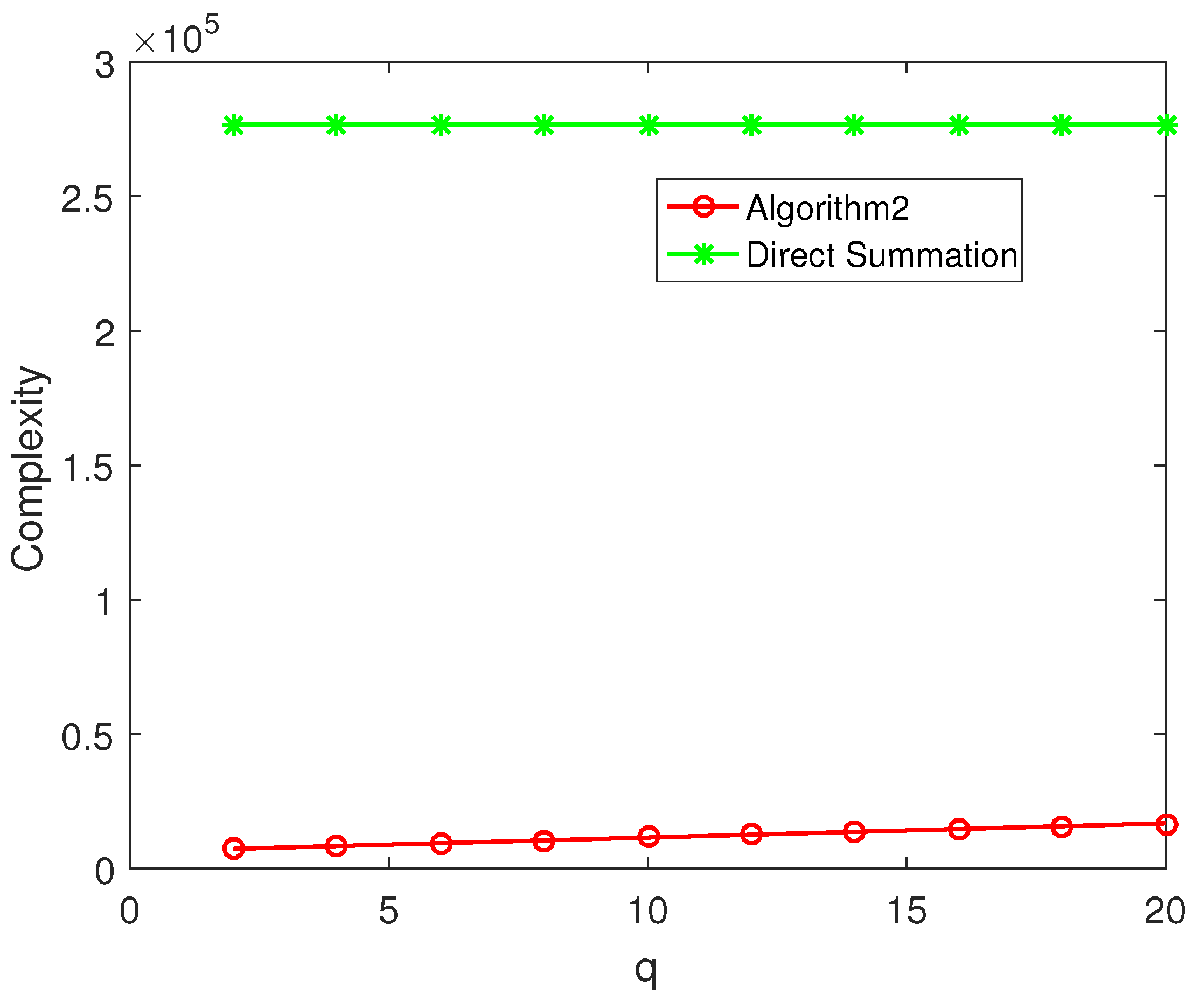
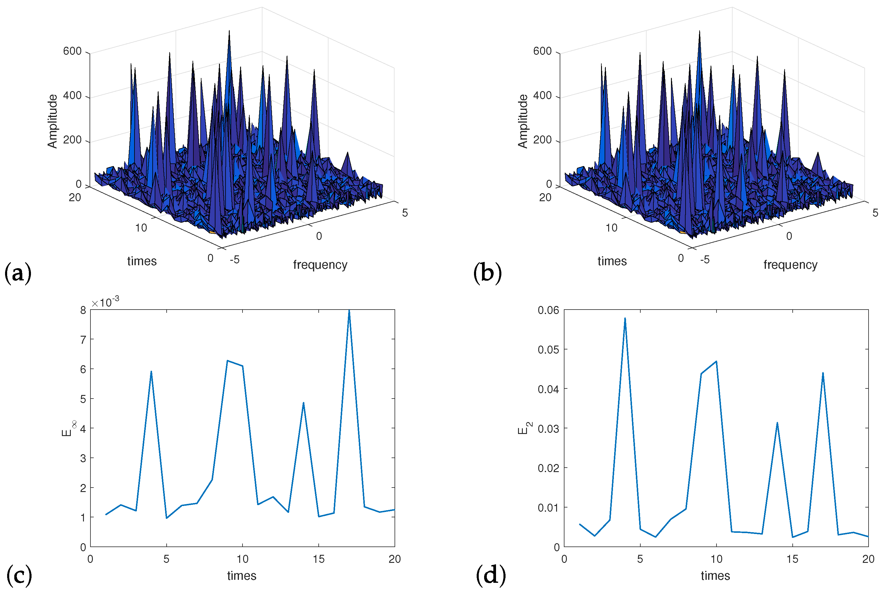
We take the parameters $a=2,b=1,c=7,d=4$, the interpolate factors $m=2$, the terms of LCS $q=10$, $\alpha =0.646$. For $N=64$, we loop our algorithm 20 times, the results are presented in Figure 1. It shows that the Algorithm 2 has almost the same effective as the direct method. For different N, the results of $E_{\infty }$ and $E_2$ are showed in Table 2. It suggested that the precision of the Algorithm 2 is independent N. For different $\alpha$ and q, the errors are presented in Table 3. It shows that the lager $\alpha$ and q is, the more accuracy of the Algorithm 2 is, and the rate of accuracy improvement is decreasing. The complexity of the Algorithm 2 dependents q and N. For $m=2$ and different q, the calculation is plotted in Figure 2. Therefore, we should not choose too big q according to the accuracy and complexity.

Figure 1. Twenty independent experiments. Amplitude (a) obtained by directly summation Equation (10); (b) obtained by Algorithm 2. Error of amplitude between the direct summation and Algorithm 2 (c) $E_{\infty }$; (d) $E_2$.

Table 2. Errorcomparison between the direct summation Equation (9) and the Algorithm 2 in case of difference N.

N	64	128	256	512
$E_{\infty }$	$2.1569\times {10}^{-6}$	$2.0019\times {10}^{-6}$	$2.1367\times {10}^{-6}$	$2.0761\times {10}^{-6}$
$E_2$	$2.1113\times {10}^{-6}$	$2.2353\times {10}^{-6}$	$2.2271\times {10}^{-6}$	$2.0740\times {10}^{-6}$

Table 3. For fixed $N=64$, error comparison between the direct summation Equation (9) and the Algorithm 2 in case of difference $\alpha$ and q.

$(\mathit{\alpha },\mathit{q})$	(0.246, 4)	(0.446, 6)	(0.646, 10)	(0.846, 12)
$E_{\infty }$	$0.0016$	$2.8818\times {10}^{-4}$	$2.4913\times {10}^{-6}$	$1.0767\times {10}^{-6}$
$E_2$	$0.0023$	$2.5009\times {10}^{-4}$	$2.2433\times {10}^{-6}$	$1.1986\times {10}^{-6}$

Figure 2. When $m=2,N=526$, complexity comparison between Algorithm 2 and direct summation for different q.

Example 3.

Here we consider the transformation $G:C^N\to C^N$ of the Problem 3 as defined Equation (10). In this example, $t_0,\cdots ,t_{N-1}$ were randomly distributed on the interval $[-b\pi ,b\pi ]$, $u_0,\cdots ,u_{N-1}$ were randomly distributed on the interval $[-N/2,N/2]$, and

$${\gamma }_k=2e^{i0.4u_k^2+i2u_k}+e^{i0.4u_k^2+i4u_k}+e^{i0.4u_k^2-i4u_k}$$

(69)

where $k=0,1\cdots ,N-1$, $a=0.234, b=1.5, c=-0.5835, d=0.5333$; interpolation factor $m=2$; the terms of the linear canonical series $q=8$ and the constant $\alpha =0.245$.

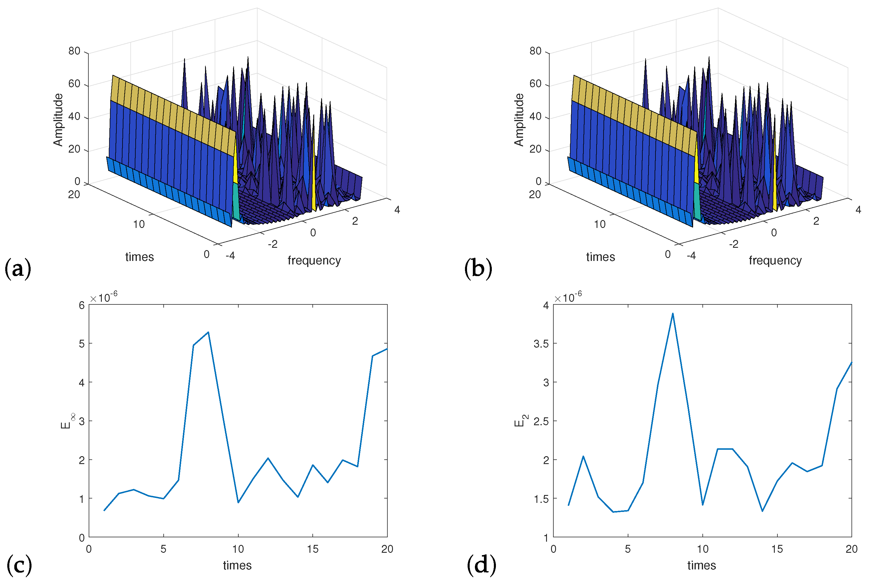
For $N=512$, the Figure 3 shows the amplitude and error for this problem by direct summation Equation (10) and Algorithm 3, respectively. It suggested that the Algorithm 3 has the almost same performance as the direct method. For different N, the Table 4 shows the error $E_{\infty }$ and $E_2$ between direct method and Algorithm 3 by cyclic algorithms 20 times. The results show that the precision of Algorithm 3 is almost independent of the length of input data.

Figure 3. Twenty independent experiments. Amplitude (a) obtained by directly summation Equation (10); (b) obtained by Algorithm 3. Error of amplitude between the direct summation and Algorithm 3 (c) $E_{\infty }$; (d) $E_2$.

Table 4. The error $E_{\infty }$ and $E_2$ between direct method and Algorithm 3 by cyclic algorithms 20 times.

N	64	128	256	512	1024
$E_{\infty }$	$0.0089$	$0.0033$	$0.0025$	$0.0014$	$0.0014$
$E_2$	$0.0343$	$0.0166$	$0.0162$	$0.0067$	$0.0102$

From the above three examples, the errors produced by Algorithms 1–3 are comparable with those produced by the corresponding direct methods. we can see that the numerical results coincide with the theoretical analyses which show the high efficiency of the new method.

The results of this paper can be generalized in the following ways: the algprithms of 1, 2 and 3 will allow the efficient application of linear transform $F_1,G_1,H_1:C^N\to C^M$ defined by

$$F_1{(\mathsf{\alpha })}_j=\sum _{k=0}^{N-1}{\alpha }_k{e}^{-i\frac{a}{2b}{(\frac{2b\pi j}{N})}^2+i\frac{u_k}{b}\frac{2\pi j}{N}-i\frac{d}{2b}{u}_k^2}$$

(70)

for $j=-M/2,\cdots ,M/2-1$, and

$$G_1{(\mathbf{g})}_j=\sum _{k=-N/2}^{N/2-1}{\beta }_k{e}^{-i\frac{a}{2b}{t}_j^2+i\frac{k{t}_j}{b}-i\frac{d}{2b}{k}^2}$$

(71)

For $j=0,1,\cdots ,M-1$, we will also consider the more general transformation $H:C^N\to C^N$ defined by the formula

$$H_1{(\mathsf{\gamma })}_j=\sum _{k=0}^{N-1}{\gamma }_k{e}^{-i\frac{a}{2b}{t}_j^2+i\frac{u_k{t}_j}{b}-i\frac{d}{2b}{u}_k^2}$$

(72)

The algorithms ofthis paper also assume that $u_k\in (-N/2,N/2), t_j\in (-b\pi ,b\pi )$. Other distributions can be handle by partitioning the vectors u and t,treating each partition separately and finally combining the results.

5. Conclusions

In this paper, we have described three algorithms for computing DLCT for nonequispaced data based on the interpolation formulae and approximation theory, which transform a function values from equispace to nonequispaced points. The complexity and precision of derived algorithms are also presented. The simulation shows that the derived approach is effective for computing nonuniform DLCT. The proposed algorithm can be viewed as generalizations of discrete linear canonical transform, and will have a broad range of applications in many branches of mathematics, science and engineering.

References

- Moshinsky, M. Linear canonical transformations and their unitary representations. J. Math. Phys. 1971, 12, 1772–1780. [Google Scholar] [CrossRef]
- Collins, S.A. Lens-System Diffraction Integral Written in Terms of Matrix Optics. J. Opt. Soc. Am. 1970, 60, 1168–1177. [Google Scholar] [CrossRef]
- Gbur, G. Simulating fields of arbitrary spatial and temporal coherence. Opt. Express 2006, 14, 7567–7578. [Google Scholar] [CrossRef] [PubMed]
- Ozaktas, H.M.; Kutay, M.A.; Zalevsky, Z. The Fractional Fourier Transform with Applications in Optics and Signal Processing; John Wiley and Sons: Hoboken, NJ, USA, 1995. [Google Scholar]
- Yan, F.J.; Li, B.Z. Windowed fractional Fourier transform on graphs: Properties and fast algorithm. Digit. Signal Process. 2021, 118, 103210. [Google Scholar] [CrossRef]
- Healy, J.J.; Kutay, M.A.; Haldun, M.; Ozaktas, H.M.; Sheridan, J.T. Linear Canonical Transforms Theory and Applications; Springer: Berlin/Heidelberg, Germany, 2016. [Google Scholar]
- Davies, B. Intergral Transforms and Their Applications; Springer: New York, NY, USA, 1978. [Google Scholar]
- Ozaktas, H.M.; Hesselink, L. Fast and accurate algorithms for quadratic phase integrals in optics and signal processing. Proc. Spie 2011, 8043, 1–12. [Google Scholar]
- Moshinsky, M. Canonical transformations and Quantum mechanics. SIAM J. Appl. Math. 1973, 25, 193–212. [Google Scholar] [CrossRef]
- Huang, X.; Zhang, L.R.; Li, S.; Zhao, Y. Radar high speed small target detection based on keystone transform and linear canonical transform. Digit. Signal Process. 2018, 82, 203–215. [Google Scholar] [CrossRef]
- Guo, Y.; Li, B.Z. Blind image watermarking method based on linear canonical wavelet transform and QR decomposition. IET Image Process. 2016, 10, 773–786. [Google Scholar] [CrossRef]
- Zhao, J.; Tao, R.; Li, Y.L.; Wang, Y. Uncertainty Principles for Linear Canonical Transform. IEEE Trans. Signal Process. 2009, 57, 2856–2858. [Google Scholar] [CrossRef]
- Zhang, Z.C. Uncertainty principle for linear canonical transform using matrix decomposition of absolute spread matrix—ScienceDirect. Digit. Signal Process. 2019, 89, 145–154. [Google Scholar] [CrossRef]
- Tao, Z.C.Z.; Li, B.Z.; Wang, Y.; Aggrey, G.K. Jittered Sampling in Linear Canonical Domain. IEEE Commun. Lett. 2020, 24, 1529–1533. [Google Scholar]
- Pei, S.C.; Ding, J.J. Closed-form discrete fractional and affine Fourier transforms. IEEE Trans. Signal Process. 2000, 48, 1338–1353. [Google Scholar]
- Zhao, J.; Tao, R.; Wang, Y. Sampling rate conversion for linear canonical transform. Signal Process. 2008, 88, 2825–2832. [Google Scholar] [CrossRef]
- Koc, A.; Ozaktas, H.M.; Candan, C.; Kutay, M.A. Digital Computation of Linear Canonical Transforms. IEEE Trans. Signal Process. 2008, 56, 2383–2394. [Google Scholar] [CrossRef]
- Oktem, F.S.; Ozaktas, H.M. Exact Relation Between Continuous and Discrete Linear Canonical Transforms. IEEE Signal Process. Lett. 2009, 16, 727–730. [Google Scholar] [CrossRef]
- Pei, S.C.; Huang, S.G. Fast Discrete Linear Canonical Transform Based on CM-CC-CM Decomposition and FFT. IEEE Trans. Signal Process. 2016, 64, 855–866. [Google Scholar] [CrossRef]
- Hennelly, B.M.; Sheridan, J.T. Fast numerical algorithm for the linear canonical transform. J. Opt. Soc. Am. Opt. Image Sci. Vis. 2005, 22, 928–937. [Google Scholar] [CrossRef]
- Healy, J.J.; Sheridan, J.T. Sampling and discretization of the linear canonical transform. Signal Process. 2009, 89, 641–648. [Google Scholar] [CrossRef]
- Stern, A. Why is the Linear Canonical Transform so little known? AIP Conf. Proc. 2006, 860, 225–234. [Google Scholar]
- Healy, J.J.; Sheridan, J.T. Fast linear canonical transforms. J. Opt. Soc. Am. Opt. Image Sci. Vis. 2010, 27, 21–30. [Google Scholar] [CrossRef] [PubMed]
- Zhang, W.L.; Li, B.Z.; Cheng, Q.Y. A New Discretization Algorithm of Linear Canonical Transform. Procedia Eng. 2012, 29, 930–934. [Google Scholar] [CrossRef][Green Version]
- Zhang, F.; Tao, R.; Wang, Y. Discrete linear canonical transform computation by adaptive method. Opt. Express 2013, 21, 18138–18151. [Google Scholar] [CrossRef] [PubMed]
- Healy, J.J.; Sheridan, J.T. Reevaluation of the direct method of calculating Fresnel and other linear canonical transforms. Opt. Lett. 2010, 35, 947–949. [Google Scholar] [CrossRef] [PubMed]
- Pei, S.C.; Lai, Y.C. Discrete linear canonical transforms based on dilated Hermite functions. J. Opt. Soc. Am. Opt. Image Sci. Vis. 2011, 28, 1695–1708. [Google Scholar] [CrossRef] [PubMed]
- Wei, D.Y.; Yang, J. Non-Uniform Sparse Fourier Transform and Its Applications. IEEE Trans. Signal Process. 2022, 70, 4468–4482. [Google Scholar] [CrossRef]
- Campos, R.G.; Figueroa, J. A fast algorithm for the linear canonical transform. Signal Process. 2011, 91, 1444–1447. [Google Scholar] [CrossRef]
- Sun, Y.N.; Li, B.Z. Digital computation of linear canonical transform for local spectra with flexible resolution ability. Sciece China. Inf. Sci. 2019, 62, 49301. [Google Scholar] [CrossRef]
- Sun, Y.N.; Li, B.Z. Sliding Discrete Linear Canonical Transform. IEEE Trans. Signal Process. 2018, 66, 4553–4563. [Google Scholar] [CrossRef]
- Sun, Y.N.; Li, B.Z. Segmented fast linear canonical transform. J. Opt. Soc. Am. Opt. Image Sci. Vis. 2018, 35, 1346–1355. [Google Scholar] [CrossRef]
- Koc, A.; Ozaktas, H.M. Operator theory-based computation of linear canonical transforms. Signal Process. 2021, 189, 108291. [Google Scholar] [CrossRef]
- Wei, D.Y.; Shen, Y. Discrete Complex Linear Canonical Transform Based on Super-differential Operators. Opt. Int. J. Light Electron Opt. 2021, 230, 166343. [Google Scholar] [CrossRef]
- Koç, A.; Ozaktas, H.M.H.L. Fast and accurate computation of two-dimensional non-separable quadratic-phase integrals. J. Opt. Soc. Am. Opt. Image Sci. Vis. 2010, 27, 1288–1302. [Google Scholar] [CrossRef] [PubMed]
- Wei, D.Y.; Hu, H. Sparse Discrete Linear Canonical Transform and Its Applications. Signal Process. 2021, 183, 108046. [Google Scholar] [CrossRef]
- Zhao, W.K.; Kintak, U.; Luo, H. Adaptive non-uniform partition algorithm based on linear canonical transform. Chaos Solitons Fractals 2022, 163, 112561. [Google Scholar] [CrossRef]
- Koç, A.; Bartan, B.; Ozaktas, H.M. Discrete Linear Canonical Transform Based on Hyperdifferential Operators. IEEE Trans. Signal Process. 2019, 67, 2237–2248. [Google Scholar] [CrossRef]
- Zhang, Y.; Li, B.Z. Discrete linear canonical transform on graphs. Digit. Signal Process. 2023, 135, 103934. [Google Scholar] [CrossRef]
- Li, C.P.; Li, B.Z.; Xu, T.Z. Approximating bandlimited signals associated with the LCT domain from nonuniform samples at unknown locations. Signal Process. 2012, 92, 1658–1664. [Google Scholar] [CrossRef]
- Wimp, J.; Gradshteyn, I.S.; Ryzhik, I.M.; Jeffrey, A. Table of Integrals, Series and Products. Am. Math. Mon. 1997, 104, 373. [Google Scholar]
Disclaimer/Publisher’s Note: The statements, opinions and data contained in all publications are solely those of the individual author(s) and contributor(s) and not of MDPI and/or the editor(s). MDPI and/or the editor(s) disclaim responsibility for any injury to people or property resulting from any ideas, methods, instructions or products referred to in the content. |
© 2023 by the authors. Licensee MDPI, Basel, Switzerland. This article is an open access article distributed under the terms and conditions of the Creative Commons Attribution (CC BY) license (https://creativecommons.org/licenses/by/4.0/).