Article

Exploring Dynamics and Hopf Bifurcation of a Fractional-Order Bertrand Duopoly Game Model Incorporating Both Nonidentical Time Delays

1
School of Mathematics and Statistics, Henan University of Science and Technology, Luoyang 471023, China
2
Guizhou Key Laboratory of Economics System Simulation, Guizhou University of Finance and Economics, Guiyang 550025, China
*
Author to whom correspondence should be addressed.
Fractal Fract. 2023, 7(5), 352; https://doi.org/10.3390/fractalfract7050352
Submission received: 20 March 2023 / Revised: 19 April 2023 / Accepted: 20 April 2023 / Published: 26 April 2023

Abstract

:
In order to maximize benefits, oligopolistic competition often occurs in contemporary society. Establishing the mathematical models to reveal the law of market competition has become a vital topic. In the current study, on the basis of the earlier publications, we propose a new fractional-order Bertrand duopoly game model incorporating both nonidentical time delays. The dynamics involving existence and uniqueness, non-negativeness, and boundedness of solution to the considered fractional-order Bertrand duopoly game model are systematacially analyzed via the Banach fixed point theorem, mathematical analysis technique, and construction of an appropriate function. Making use of different delays as bifurcation parameters, several sets of new stability and bifurcation conditions ensuring the stability and the creation of Hopf bifurcation of the established fractional-order Bertrand duopoly game model are acquired. By virtue of a proper definite function, we set up a new sufficient condition that ensures globally asymptotically stability of the considered fractional-order Bertrand duopoly game model. The work reveals the impact of different types of delays on the stability and Hopf bifurcation of the proposed fractional-order Bertrand duopoly game model. The study shows that we can adjust the delay to achieve price balance of different products. To confirm the validity of the derived criteria, we put computer simulation into effect. The derived conclusions in this article are wholly new and have great theoretical value in administering companies.

1. Introduction

In the market, when homogeneous goods are produced by several different companies, oligopolistic competition will easily take place. In order to pursue the maximization of various benefits, the companies take the best measures and perform everything possible to achieve the established goal. Thus, the duopoly game has become normal. Revealing the duopoly game law of different companies is an extremely significative topic. Mathematically speaking, a suitable research topic is to build mathematical models to probe into the relationship among variables. During the past decades, there have been a great deal of meaningful and interesting publications that are concerned with various duopoly game models. For instance, Zhang et al. [1] dealt with the stability behavior and Hopf bifurcation of a Bertrand model involving bounded rationality. Yu and Yu [2] explored the local stability and the global stability of a Bertrand duopoly model involving comprehensive preference. They established the sufficient conditions to ensure the local stability and global stability of a Bertrand duopoly model. Cao et al. [3] investigated the local stability of the equilibria, global bifurcation, and synchronization of a duopoly game model concerning bounded rationality and consumer surplus. Baiardi and Naimzada [4] studied the local stability and Neimark–Sacker bifurcations of an oligopoly model. Zhu et al. [5] carried out a theoretical analysis on stability, coexistence of attractors, and contact bifurcation for a Cournot–Bertrand duopoly game model involving heterogeneous players. Askar and Al-khedhairi [6] implemented concrete discussion on local and global stability of the equilibrium points for a duopoly game concerning price competition. For more detailed works on this aspect, one can see the literature [7,8,9,10,11,12,13,14,15].
The price of products is one of the important factors that affects the competition among different companies. The price has a vital influence on the distribution of products and the demand from people [16]. Adjusting the price of products effectively has become a central issue for companies. To this day, a lot of valuable scientific achievements about this topic have been available. For instance, Wang and Hou [17] investigated a duopoly game model with heterogeneous green supply chains in optimal price and market stability with consumer green preference. They revealed the effect of consumer green preference on members’ optimal decisions and the speed of the adjustment of the optimal price strategies for heterogeneous green supply chains. Safarzadeh et al. [18] explored the duopoly pricing of energy-efficient appliances regarding innovation protection and social welfare via a game theoretic approach. Huang et al. [19] discussed the equilibrium issue of pricing competition and cooperation in supply chain involving one common manufacturer and duopoly retailers. Mukhopadhyay et al. [20] analyzed a Stackelberg price model of complementary goods under information asymmetry. In 2016, Ma and Si [21] set up the following Bertrand duopoly game model incorporating both nonidentical time delays:
q ˙ 1 ( t ) = μ 1 q 1 ( t ) [ α 1 2 β 1 ϖ q 1 ( t ρ 1 ) 2 β 1 ( 1 ϖ ) q 1 ( t ρ 2 ) + δ 1 q 2 ( t ) + β 1 γ 1 ] , q ˙ 2 ( t ) = μ 2 q 2 ( t ) [ α 2 2 β 2 q 2 ( t ) + δ 2 ϖ q 1 ( t ρ 1 ) + δ 2 ( 1 ϖ ) q 1 ( t ρ 2 ) + β 2 γ 2 ] ,
where q 1 ( t ) represents the price of the company I, q 2 ( t ) represents the price of the company II, μ 1 denotes the speed of price adjustment of the company I, μ 2 denotes the speed of price adjustment of the company II, α 1 and α 2 denote the basic demand for the market, β 1 and β 2 represent the elastic demand for its itself, and γ 1 and γ 2 represent the marginal costs of company I, company II, respectively. ϖ [ 0 , 1 ] is the weight of price at time t ρ 1 , 1 ϖ is the weight of price at time t ρ 2 , ρ 1 represents a time delay, and all the coefficients μ i , α i , β i , γ i , δ 1 , ρ i ( i = 1 , 2 ) , ϖ are positive constants. For more details, we refer to the readers to [21]. By selecting the time delay as bifurcation parameter, Ma and Si [21] obtained the bifurcation value of model (1). By virtue of the power spectrum, attractor, bifurcation diagram, the largest Lyapunov exponent, 3D surface chart, 4D Cubic Chart, 2D parameter bifurcation diagram, and 3D parameter bifurcation diagram [21], the dynamical behaviors of the model (1) are displayed.
Here, we must mention that all the above works on duopoly game models (see [1,2,3,4,5,6,7,8,9,10,11,12,13,14,15,16,17,18,19,20,21]) merely focus on the integer-order differential models. A number of studies have shown that fractional-order differential systems own more degrees of freedom and longer-range interactivity in time and space [22,23,24]. The majority of biological, neural network, economic, physical, chemical, and engineering systems own long-range temporal memory or/and long-range space interplay [25]. Thus, describing these biological, economic, physical, chemical and engineering systems and neural networks by virtue of fractional-order differential equations owns more advantages than traditional integer-order ones since the influence of time memory and long-range space interplay can be revealed [25]. Nowadays, fractional-order differential systems have displayed potential applications in many fields such as neural networks, biological technique, control science, physics, chemistry, capacitor principle, electrical engineering, economics, etc. [26,27,28,29,30,31]. To this day, many scholars have concentrated on fractional-order dynamical systems and achieved very gratifying results. For example, Huang et al. [31] probed into Hopf bifurcation of fractional-order BAM neural networks with multiple time delays. Alidousti [32] analyzed the stability behavior and Hopf bifurcation of a fractional-order predator–prey scavenger system. Zhang et al. [33] dealt with the dynamical bifurcation of large scale delayed fractional-order neural networks involving hub structure and multiple rings. Eshaghi et al. [29] discussed the bifurcation, synchronization, and chaos control of a fractional-order chaotic system. For more details, one can see [29,34,35,36,37,38,39,40,41,42].
Stimulated by the idea above and on the basis of model (1), in this present research, we are to build the following fractional-order Bertrand duopoly game model:
D ϱ q 1 ( t ) = μ 1 q 1 ( t ) [ α 1 2 β 1 ϖ q 1 ( t ρ 1 ) 2 β 1 ( 1 ϖ ) q 1 ( t ρ 2 ) + δ 1 q 2 ( t ) + β 1 γ 1 ] , D ϱ q 2 ( t ) = μ 2 q 2 ( t ) [ α 2 2 β 2 q 2 ( t ) + δ 2 ϖ q 1 ( t ρ 1 ) + δ 2 ( 1 ϖ ) q 1 ( t ρ 2 ) + β 2 γ 2 ] ,
where ϱ ( 0 , 1 ] . All other coefficients and variables have the same implication as those in Bertrand duopoly game model (1). The model (2) has more advantages than model (1) since it can better describe the memory trait and hereditary nature of the prices of two companies. By considering the different delay cases, we can reveal the effect of different delays on the change of the prices of two companies, which can help us to manage and operate enterprises with a flexible and efficient way. For example, we can control the values of the two delays ρ 1 , ρ 2 to realize the stability of the prices of two companies or balance of the prices of two companies. In addition, for different delay cases, we can choose a suitable fractional order parameter to seek the critical value of delay which ensures the periodic motion of the prices of two companies. Based on this exploration, we think that the investigation on the dynamics of model (2) owns very important practical significance in corporate governance.
In this current research, we predominantly explore the following three aspects:
(1)
Explore the existence and uniqueness, non-negativeness, and boundedness of the solution to the fractional-order Bertrand duopoly game model (2).
(2)
Seek a series of delay-independent sufficient criteria that ensures the stability and the creation of Hopf bifurcation of the fractional-order Bertrand duopoly game model (2).
(3)
Build the sufficient condition that guarantees the globally asymptotically stability of the fractional-order Bertrand duopoly game model (2).
The key highlights of this research are expounded as follows:
  • Based on the studies of predecessors, a new fractional-order Bertrand duopoly game model is established.
  • A series of delay-independent sufficient criteria that ensures the stability and the creation of Hopf bifurcation of the fractional-order Bertrand duopoly game model (2) with different types of delay is derived.
  • The sufficient criterion that ensures the globally asymptotically stability of the fractional-order Bertrand duopoly game model (2) is derived by virtue of construction of a suitable positive definite function skillfully.
  • The impact of delay on the stability and the occurrence of Hopf bifurcation of the fractional-order Bertrand duopoly game model (2) is elaborated.
  • The study ideas can provide reference for us to probe into the bifurcation problem of plentiful fractional dynamical systems in many fields.
This article is planned as follows. In Section 2, we give requisite theory on the fractional-order dynamical system. In Section 3, the proofs of the existence and uniqueness, boundedness, non-negativeness, and boundedness of the solution to the fractional-order Bertrand duopoly game model (2) are presented. In Section 4, a series of delay-independent sufficient criteria ensuring the stability and the onset of Hopf bifurcation of the fractional-order Bertrand duopoly game model (2) with different types of delay are built. In Section 5, the globally asymptotically stability of the fractional-order Bertrand duopoly game model (2) is explored. In Section 6, numerical simulations are implemented to sustain the derived primary results. In Section 7, we give a conclusion to end this work.
Remark 1. 
In model (2), we define the order ϱ ( 0 , 1 ] which stands for the first order fractional operator.

2. Preliminaries

In this segment, some essential basic theories about fractional-order differential equations are presented.
Definition 1 
([43]). Define the fractional integral of order ϱ of the function h ( r ) as follows:
I ϱ h ( r ) = 1 Γ ( ϱ ) r 0 r ( r τ ) ϱ 1 h ( τ ) d τ ,
where r > r 0 ,   ϱ > 0 ,   Γ ( τ ) = 0 s τ 1 e s d s , which represents the Gamma function.
Definition 2 
([44]). The Caputo fractional-order derivative of order ϱ of the function h ( r ) ( [ r 0 , ) , R ) is given by
D ϱ h ( r ) = 1 Γ ( ι ϱ ) r 0 r h ( l ) ( s ) ( r s ) ϱ l + 1 d s ,
where ϵ ϵ 0 and l stands for a positive integer ( l 1 ϱ < l ) . In particular, when ϱ ( 0 , 1 ) , then one has D ϱ h ( r ) = 1 Γ ( 1 ϱ ) r 0 r h ( s ) ( r s ) ϱ d s .
Lemma 1 
([45]). For the following fractional system: D ϱ x = H x , x ( 0 ) = x 0 where ϱ ( 0 , 1 ) , x R n , Q R n × n , denote χ l ( l = 1 , 2 , , n ) the root of the characteristic equation of D ϱ x = H x . Then, system D ϱ x = H x is locally asymptotically stable ⇔ | a r g ( χ l ) | > ϱ π 2 ( l = 1 , 2 , , n ) . The system is stable ⇔ | a r g ( χ l ) | > ϱ π 2 ( l = 1 , 2 , , n ) and all critical eigenvalues, which satisfy | a r g ( χ l ) | = ϱ π 2 ( l = 1 , 2 , , n ) , have geometric multiplicity one.
Lemma 2 
([46]). Let ϱ ( 0 , 1 ] , h ( t ) C [ c 1 , c 2 ] and D ϱ h ( t ) C [ a 1 , a 2 ] . Suppose that D ϱ h ( t ) 0 , t ( c 1 , c 2 ) . Then, h ( t ) is a non-decreasing function for t [ c 1 , c 2 ] . Suppose that D ϱ h ( t ) 0 , t ( c 1 , c 2 ) . Then, h ( t ) is a non-increasing function for t [ c 1 , c 2 ] .
Lemma 3 
([45]). Assume that ϖ ( t ) C [ t 0 , ) and satisfies
D ϱ ϖ ( t ) ϑ 1 ϖ ( t ) + ϑ 2 , ϖ ( t 0 ) = ϖ t 0 ,
where ϱ ( 0 , 1 ) , ϑ 1 , ϑ 2 R , ϑ 1 0 , t 0 0 . Then,
ϖ ( t ) ϖ ( t 0 ) ϑ 2 ϑ 1 E ϱ [ ϑ 1 ( t t 0 ) ϱ ] + ϑ 2 ϑ 1 .

3. Dynamics Exploration of the Solution

In this part, we will probe into the existence and uniqueness, non-negativeness, and boundedness of the solution to system (2) via the Banach fixed point theorem and Lemma 2.
Theorem 1. 
Denote Y = { q 1 , q 2 ) R 2 : max { | q 1 | , | q 2 | } Q } , where Q > 0 represents a constant. For each ( q 10 , q 20 ) Y , system (2) with the initial condition ( q 10 , q 20 ) owns a unique solution Q = ( q 1 , q 2 ) Y .
Proof. 
Define a mapping as follows:
g ( Q ) = ( g 1 ( Q ) , g 2 ( Q ) ) ,
where
g 1 ( Q ) = μ 1 q 1 ( t ) [ α 1 2 β 1 ϖ q 1 ( t ρ 1 ) 2 β 1 ( 1 ϖ ) q 1 ( t ρ 2 ) + δ 1 q 2 ( t ) + β 1 γ 1 ] , g 2 ( Q ) = μ 2 q 2 ( t ) [ α 2 2 β 2 q 2 ( t ) + δ 2 ϖ q 1 ( t ρ 1 ) + δ 2 ( 1 ϖ ) q 1 ( t ρ 2 ) + β 2 γ 2 ] .
Q , Q ¯ Y , one has
| | g ( Q ) g ( Q ¯ ) | | = μ 1 q 1 ( t ) [ α 1 2 β 1 ϖ q 1 ( t ρ 1 ) 2 β 1 ( 1 ϖ ) q 1 ( t ρ 2 ) + δ 1 q 2 ( t ) + β 1 γ 1 ] μ 1 q ¯ 1 ( t ) [ α 1 2 β 1 ϖ q ¯ 1 ( t ρ 1 ) 2 β 1 ( 1 ϖ ) q ¯ 1 ( t ρ 2 ) + δ 1 q ¯ 2 ( t ) + β 1 γ 1 ] + μ 2 q 2 ( t ) [ α 2 2 β 2 q 2 ( t ) + δ 2 ϖ q 1 ( t ρ 1 ) + δ 2 ( 1 ϖ ) q 1 ( t ρ 2 ) + β 2 γ 2 ] μ 2 q ¯ 2 ( t ) [ α 2 2 β 2 q ¯ 2 ( t ) + δ 2 ϖ q ¯ 1 ( t ρ 1 ) + δ 2 ( 1 ϖ ) q ¯ 1 ( t ρ 2 ) + β 2 γ 2 ] μ 1 α 1 | q 1 ( t ) q ¯ 1 ( t ) | + 4 μ 1 β 1 ϖ Q | q 1 ( t ) q ¯ 1 ( t ) | + 4 μ 1 β 1 ( 1 ϖ ) | q 1 ( t ) q ¯ 1 ( t ) | + μ 1 δ 1 Q | q 1 ( t ) q ¯ 1 ( t ) | + μ 1 δ 1 Q | q 2 ( t ) q ¯ 2 ( t ) | + μ 1 β 1 γ 1 | q 1 ( t ) q ¯ 1 ( t ) | + μ 2 α 2 | q 2 ( t ) q ¯ 2 ( t ) | + 4 μ 2 β 2 ϖ Q | q 2 ( t ) q ¯ 2 ( t ) | + μ 2 δ 2 ϖ Q | q 1 ( t ) q ¯ 1 ( t ) | + μ 2 δ 2 ϖ Q | q 2 ( t ) q ¯ 2 ( t ) | + μ 2 δ 2 ( 1 ϖ ) Q | q 1 ( t ) q ¯ 1 ( t ) | + μ 2 δ 2 ( 1 ϖ ) Q | q 2 ( t ) q ¯ 2 ( t ) | + μ 2 β 2 γ 2 | q 2 ( t ) q ¯ 2 ( t ) | = μ 1 α 1 + 4 μ 1 β 1 ϖ Q + 4 μ 1 β 1 ( 1 ϖ ) + μ 1 δ 1 Q + μ 1 β 1 γ 1 + μ 2 δ 2 Q | q 1 ( t ) q ¯ 1 ( t ) | + [ μ 1 δ 1 Q + μ 2 α 2 + 4 μ 2 β 2 ϖ Q + μ 2 δ 2 Q + μ 2 β 2 γ 2 ] | q 2 ( t ) q ¯ 2 ( t ) | = Q 1 | q 1 ( t ) q ¯ 1 ( t ) | + Q 2 | q 2 ( t ) q ¯ 2 ( t ) | Q | | Q Q ¯ | | ,
where
Q 1 = μ 1 α 1 + 4 μ 1 β 1 ϖ Q + 4 μ 1 β 1 ( 1 ϖ ) + μ 1 δ 1 Q + μ 1 β 1 γ 1 + μ 2 δ 2 Q , Q 2 = μ 1 δ 1 Q + μ 2 α 2 + 4 μ 2 β 2 ϖ Q + μ 2 δ 2 Q + μ 2 β 2 γ 2 ,
and
Q = max { Q 1 , Q 2 } .
Then, g ( Q ) satisfies the Lipschitz condition with respect to Q (see [45]). Making use of the Banach fixed point theorem [47], we can obtain that Theorem 1 holds true.
Theorem 2. 
(1) Each solution of model (2) beginning with R + 2 is non-negative; (2) If min { 2 μ 1 β 1 ϖ , 2 μ 2 β 2 } > 1 2 μ 1 δ 1 + 1 2 μ 2 δ 2 ( 1 ϖ ) , then each solution of model (2) beginning with R + 2 is uniformly bounded.
Proof. 
Denote Q ( t 0 ) = ( q 1 ( t 0 ) , q 2 ( t 0 ) ) the initial condition of model (2). Suppose that ∃ a constant t , which satisfies t ( t 0 , t ) , such that
q 1 ( t ) > 0 , t ( t 0 , t ) , q 1 ( t ) = 0 , q 1 ( t + ) < 0 .
In view of model (2), one has
D ϱ q 1 ( t ) | q 1 ( t ) = 0 = 0 .
According to Lemma 2, we obtain q 1 ( t + ) = 0 . In view of (8), it is a contradiction. So, q 1 ( t ) 0 , ∀ t t 0 . In a similar way, we can also prove that q 2 ( t ) 0 , ∀ t t 0 . The proof of (1) finishes. Next, we are to prove uniformly boundedness of model (2). Let
Ξ ( t ) = q 1 ( t ) + q 2 ( t ) .
Then
D ϱ Ξ ( t ) + k Ξ ( t ) = D ϱ q 1 ( t ) + D ϱ q 2 ( t ) + k q 1 ( t ) + k q 2 ( t ) = μ 1 q 1 ( t ) [ α 1 2 β 1 ϖ q 1 ( t ρ 1 ) 2 β 1 ( 1 ϖ ) q 1 ( t ρ 2 ) + δ 1 q 2 ( t ) + β 1 γ 1 ] + μ 2 q 2 ( t ) [ α 2 2 β 2 q 2 ( t ) + δ 2 ϖ q 1 ( t ρ 1 ) + δ 2 ( 1 ϖ ) q 1 ( t ρ 2 ) + β 2 γ 2 ] + κ y 1 ( t ) + κ y 2 ( t ) ( μ 1 α 1 + μ 1 β 1 γ 1 + k ) q 1 ( t ) 2 μ 1 β 1 ϖ q 1 2 ( t ) + μ 1 δ 1 q 1 ( t ) q 2 ( t ) + ( μ 2 α 2 + μ 2 β 2 γ 1 + k ) q 2 ( t ) 2 μ 2 β 2 q 2 2 ( t ) + μ 2 δ 2 ( 1 ϖ ) q 1 ( t ) q 2 ( t ) ( μ 1 α 1 + μ 1 β 1 γ 1 + k ) q 1 ( t ) 2 μ 1 β 1 ϖ q 1 2 ( t ) + 1 2 μ 1 δ 1 q 1 2 ( t ) + 1 2 μ 1 δ 1 q 2 2 ( t ) + ( μ 2 α 2 + μ 2 β 2 γ 1 + k ) q 2 ( t ) 2 μ 2 β 2 q 2 2 ( t ) + 1 2 μ 2 δ 2 ( 1 ϖ ) q 1 2 ( t ) + 1 2 μ 2 δ 2 ( 1 ϖ ) q 2 2 ( t ) = ( μ 1 α 1 + μ 1 β 1 γ 1 + k ) q 1 ( t ) 2 μ 1 β 1 ϖ 1 2 μ 1 δ 1 1 2 μ 2 δ 2 ( 1 ϖ ) q 1 2 ( t ) + ( μ 2 α 2 + μ 2 β 2 γ 1 + k ) q 2 ( t ) 2 μ 2 β 2 1 2 μ 1 δ 1 1 2 μ 2 δ 2 ( 1 ϖ ) q 2 2 ( t ) A ,
where κ > 0 is a constant and
A = 2 μ 1 β 1 ϖ 1 2 μ 1 δ 1 1 2 μ 2 δ 2 ( 1 ϖ ) 2 4 ( μ 1 α 1 + μ 1 β 1 γ 1 + k ) + 2 μ 2 β 2 1 2 μ 1 δ 1 1 2 μ 2 δ 2 ( 1 ϖ ) 2 4 ( μ 2 α + μ 2 β 2 γ 1 + k ) .
Then
D ϱ Ξ ( t ) k Ξ ( t ) + A .
According to Lemma 3, we obtain
Ξ ( t ) Ξ ( t 0 ) A k E ϱ [ k ( t t 0 ) ϱ ] + A k ,
then
Ξ ( t ) A k , a s t ,
which ends the proof of Theorem 2. □

4. Bifurcation Discussion on Model (2)

We can easily obtain the following equilibria of system (2):
Q 1 ( 0 , 0 ) , Q 2 0 , α 2 + β 2 γ 2 2 β 2 , Q 3 α 1 + β 1 γ 1 2 β 1 , 0 , Q 4 ( q 1 , q 2 ) ,
where
q 1 = 2 α 1 β 2 + 2 β 1 β 2 γ 1 + α 2 δ 1 + β 2 γ 2 δ 1 4 β 1 β 2 δ 1 δ 2 , q 2 = 2 α 2 β 1 + 2 β 1 β 2 γ 2 + α 1 δ 2 + β 1 γ 1 δ 2 4 β 1 β 2 δ 1 δ 2 .
Assume that
( N 1 ) δ 1 δ 2 < 4 β 1 β 2 ,
is satisfied. Then, the equilibrium point Q 4 ( q 1 , q 2 ) is a positive equilibrium point. Noticing the real implication of Bertrand duopoly game model, we merely analyze the positive equilibrium point Q 4 ( q 1 , q 2 ) of system (2). The linear system of system (2) at Q 4 ( q 1 , q 2 ) takes the following form:
D ϱ q ( t ) = C 1 q ( t ) + C 2 q ( t ρ 1 ) + C 3 q ( t ρ 2 ) ,
where ϱ ( 0 , 1 ] and
q ( t ) = q 1 ( t ) q 2 ( t ) , C 1 = b 1 b 2 0 b 3 , C 2 = b 4 0 b 5 0 , C 3 = b 6 0 b 7 0 ,
where
b 1 = μ 1 α 1 + μ 1 β 1 γ 1 2 μ 1 β 1 ϖ q 1 + μ 1 δ 1 q 2 , b 2 = μ 1 δ 1 q 1 , b 3 = μ 2 α 2 + μ 2 β 2 γ 2 4 μ 4 β 4 q 2 + μ 2 δ 2 q 1 , b 4 = 2 μ 1 β 1 ϖ q 1 , b 5 = 2 μ 2 β 2 ϖ q 2 , b 6 = 2 μ 1 β 1 ( 1 ϖ ) q 1 , b 7 = μ 2 δ 2 ( 1 ϖ ) q 2 .
The characteristic equation of system (17) is given by
det s ϱ b 1 b 4 e s ρ 1 b 6 e s ρ 2 b 2 b 5 e s ρ 1 b 7 e s ρ 2 s ϱ b 3 = 0 .
It follows from (20) that
s 2 ϱ + d 1 s ϱ + d 2 + ( d 3 s ϱ + d 4 ) e s ρ 1 + ( d 5 s ϱ + d 6 ) e s ρ 2 = 0 ,
where
d 1 = ( b 1 + b 3 ) , d 2 = b 1 b 3 , d 3 = b 4 , d 4 = b 3 b 4 b 2 b 5 , d 5 = b 6 , d 6 = b 3 b 6 b 2 b 7 .
In the sequel, we are to explore six cases:
Case one. If ρ 1 = 0 , ρ 2 = 0 , then, Equation (21) is
λ 2 + ( d 1 + d 3 + d 5 ) λ + d 2 + d 4 + d 6 = 0 ,
where λ = s ϱ . If
( N 2 ) d 1 + d 3 + d 5 > 0 , d 2 + d 4 + d 6 > 0 ,
holds, then both roots λ 1 , λ 2 of Equation (23) satisfy | arg ( λ 1 ) | > ϱ π 2 , | arg ( λ 2 ) | > ϱ π 2 . By Lemma 1, one can know that the positive equilibrium point Q 4 ( q 1 , q 2 ) of system (2) with ρ 1 = 0 , ρ 2 = 0 is locally asymptotically stable.
Case two. If ρ 1 = 0 , ρ 2 > 0 , Equation (21) is
s 2 ϱ + ( d 1 + d 3 ) s ϱ + d 2 + d 4 + ( d 5 s ϱ + d 6 ) e s ρ 2 = 0 ,
Let s = i θ = θ cos π 2 + i sin π 2 be the root of Equation (24). Then, Equation (24) becomes
θ 2 ϱ ( cos ϱ π + i sin ϱ π ) + ( d 1 + d 3 ) θ ϱ cos ϱ π 2 + i sin ϱ π 2 + d 2 + d 4 + d 5 θ ϱ cos ϱ π 2 + i sin ϱ π 2 + d 6 ( cos θ ρ 2 i sin θ ρ 2 ) = 0 .
Then
A 1 cos θ ρ 2 + A 2 sin θ ρ 2 = A 3 , A 2 cos θ ρ 2 A 1 sin θ ρ 2 = A 4 ,
where
A 1 = d 5 θ ϱ cos ϱ π 2 + d 6 , A 2 = d 5 θ ϱ sin ϱ π 2 , A 3 = θ 2 ϱ cos ϱ π ( d 1 + d 3 ) θ ϱ cos ϱ π 2 ( d 2 + d 4 ) , A 4 = θ 2 ϱ sin ϱ π ( d 1 + d 3 ) θ ϱ sin ϱ π 2 .
By (26), we have
A 1 2 + A 2 2 = A 3 2 + A 4 2 ,
which leads to
θ 4 ϱ + e 1 θ 3 ϱ + e 2 θ 2 ϱ + e 3 θ ϱ + e 4 = 0 ,
where
e 1 = 2 ( d 1 + d 3 ) cos η π cos η π 2 + sin η π sin η π 2 , e 2 = 2 ( d 2 + d 4 ) cos η π + ( d 1 + d 3 ) 2 d 5 2 , e 3 = 2 [ ( d 1 + d 3 ) ( d 2 + d 4 ) d 5 d 6 ] cos η π 2 , e 4 = ( d 2 + d 4 ) 2 d 6 2 .
Let
Π 1 ( θ ) = θ 4 ϱ + e 1 θ 3 ϱ + e 2 θ 2 ϱ + e 3 θ ϱ + e 4 .
Assume that
( N 3 ) | d 2 + d 4 | < | d 6 | ,
is fulfilled, since d Π 1 ( θ ) d θ > 0 ,∀ θ > 0 . Then, we can easily conclude that Equation (29) owns at least one positive real root. Thus, Equation (24) has at least one pair of purely roots. By virtue of Sun et al. [48], we can obtain the following assertion.
Lemma 4. 
(i) Suppose that e l > 0 ( l = 1 , 2 , 3 , 4 ) is satisfied, then Equation (24) has no root with zero real parts if ρ 2 0 . (ii) Suppose that ( N 3 ) is satisfied and e l > 0 ( l = 1 , 2 , 3 ) , then Equation (24) owns a pair of purely imaginary roots ± i θ 0 when ρ 2 = ρ 2 k ( k = 1 , 2 , , ) where
ρ 20 ( k ) = 1 θ 0 arccos A 1 A 3 + A 2 A 4 A 1 2 + A 2 2 + 2 k π ,
where k = 0 , 1 , 2 , , and θ 0 > 0 stands for the unique zero of the function Π 1 ( θ ) .
For the proof of Lemma 4, we refer the readers to [48]. Set ρ 20 = ρ 20 ( 0 ) .
Next, the following hypothesis is given:
( N 4 ) E 1 R E 2 R + E 1 I E 2 I > 0 ,
where
E 1 R = 2 ϱ θ 0 2 ϱ 1 cos ( 2 ϱ 1 ) π 2 + ϱ ( d 1 + d 3 ) θ 0 ϱ 1 cos ( ϱ 1 ) π 2 + ϱ d 5 θ 0 ϱ 1 cos ( ϱ 1 ) π 2 cos θ 0 ρ 20 + sin ( ϱ 1 ) π 2 sin θ 0 ρ 20 , E 1 I = 2 ϱ θ 0 2 ϱ 1 sin ( 2 ϱ 1 ) π 2 + ϱ ( d 1 + d 3 ) θ 0 ϱ 1 sin ( ϱ 1 ) π 2 ϱ d 5 θ 0 ϱ 1 cos ( ϱ 1 ) π 2 sin θ 0 ρ 20 sin ( ϱ 1 ) π 2 cos θ 0 ρ 20 , E 2 R = d 5 θ 0 ϱ cos ϱ π 2 + d 6 θ 0 sin θ 0 ρ 20 + d 5 θ 0 ϱ cos ϱ π 2 θ 0 cos θ 0 ρ 20 , E 2 I = d 5 θ 0 ϱ cos ϱ π 2 + d 6 θ 0 sin θ 0 ρ 20 d 5 θ 0 ϱ cos ϱ π 2 θ 0 cos θ 0 ρ 20 .
Lemma 5. 
Suppose that s ( ρ 2 ) = σ 1 ( ρ 2 ) + i σ 2 ( ρ 2 ) is the root of Equation (24) at ρ 2 = ρ 20 such that σ 1 ( ρ 20 ) = 0 , σ 2 ( ρ 20 ) = θ 0 . Then, Re d s d ρ 2 | ρ 2 = ρ 20 , θ = θ 0 > 0 .
Proof. 
By Equation (24), we derive
2 ϱ s 2 ϱ 1 + ϱ ( d 1 + d 3 ) s ϱ 1 d s d ρ 2 + ϱ d 5 s ϱ 1 e s ρ 2 d s d ρ 2 e s ρ 2 d s d ρ 2 ρ 2 + s d 5 s η + d 6 = 0 ,
which implies
d s d ρ 2 1 = E 1 ( s ) E 2 ( s ) ρ 2 s ,
where
E 1 ( s ) = 2 ϱ s 2 ϱ 1 + ϱ ( d 1 + d 3 ) s ϱ 1 + ϱ d 5 s ϱ 1 e s ρ 2 , E 2 ( s ) = s e s ρ 2 [ d 5 s ϱ + d 6 ] .
Then,
Re d s d ρ 2 1 ρ 2 = ρ 20 , θ = θ 0 = Re E 1 ( s ) E 2 ( s ) ρ 2 = ρ 20 , θ = θ 0 = E 1 R E 2 R + E 1 I E 2 I E 2 R 2 + E 2 I 2 .
According to ( N 4 ) , one gets
Re d s d ρ 2 1 ρ 2 = ρ 20 , θ = θ 0 > 0 ,
which ends the proof. □
Taking advantage of exploration above, the following conclusion can be easily derived.
Theorem 3. 
Suppose that ( N 1 ) ( N 4 ) is fulfilled. Then, Q 4 ( q 1 , q 2 ) of model (2) with ρ 1 = 0 is locally asymptotically stable when ρ 2 [ 0 , ρ 20 ) and model (2) generates Hopf bifurcation around Q 4 ( q 1 , q 2 ) when ρ 2 = ρ 20 .
Case three. If ρ 2 = 0 , ρ 1 > 0 , Equation (21) is
s 2 ϱ + ( d 1 + d 5 ) s ϱ + d 2 + d 6 + ( d 3 s ϱ + d 4 ) e s ρ 1 = 0 ,
Let s = i η = η cos π 2 + i sin π 2 be the root of Equation (39). Then, Equation (39) becomes
η 2 ϱ ( cos ϱ π + i sin ϱ π ) + ( d 1 + d 5 ) η ϱ cos ϱ π 2 + i sin ϱ π 2 + d 2 + d 6 + d 3 η ϱ cos ϱ π 2 + i sin ϱ π 2 + d 4 ( cos η ρ 1 i sin η ρ 1 ) = 0 .
Then
B 1 cos η ρ 1 + B 2 sin η ρ 1 = B 3 , B 2 cos η ρ 1 B 1 sin η ρ 1 = B 4 ,
where
B 1 = d 3 η ϱ cos ϱ π 2 + d 4 , B 2 = d 3 η ϱ sin ϱ π 2 , B 3 = η 2 ϱ cos ϱ π ( d 1 + d 5 ) η ϱ cos ϱ π 2 ( d 2 + d 6 ) , B 4 = η 2 ϱ sin ϱ π ( d 1 + d 5 ) η ϱ sin ϱ π 2 .
By (41), we have
B 1 2 + B 2 2 = B 3 2 + B 4 2 ,
which leads to
η 4 ϱ + f 1 η 3 ϱ + f 2 η 2 ϱ + f 3 η ϱ + f 4 = 0 ,
where
f 1 = 2 ( d 1 + d 5 ) cos η π cos η π 2 + sin η π sin η π 2 , f 2 = 2 ( d 2 + d 6 ) cos η π + ( d 1 + d 5 ) 2 d 3 2 , f 3 = 2 [ ( d 1 + d 5 ) ( d 2 + d 6 ) d 3 d 4 ] cos η π 2 , f 4 = ( d 2 + d 6 ) 2 d 4 2 .
Let
Π 2 ( η ) = η 4 ϱ + f 1 η 3 ϱ + f 2 η 2 ϱ + f 3 η ϱ + f 4 .
Assume that
( N 5 ) | d 2 + d 6 | < | d 4 | ,
is fulfilled, since d Π 2 ( η ) d η > 0 ,∀ η > 0 . Then, we can easily conclude that Equation (44) owns at least one positive real root. Thus, Equation (39) has at least one pair of purely roots. By virtue of Sun et al. [48], we can obtain the following assertion.
Lemma 6. 
(i) Suppose that f l > 0 ( l = 1 , 2 , 3 , 4 ) is satisfied, Equation (39) has no root with zero real parts if ρ 1 0 . (ii) Suppose that ( N 5 ) is satisfied and f l > 0 ( l = 1 , 2 , 3 ) . Then, Equation (39) owns a pair of purely imaginary roots ± i η 0 when ρ 1 = ρ 1 k ( k = 1 , 2 , , ) where
ρ 10 ( k ) = 1 η 0 arccos B 1 B 3 + B 2 B 4 B 1 2 + B 2 2 + 2 k π ,
where k = 0 , 1 , 2 , , and η 0 > 0 stands for the unique zero of the function Π 2 ( η ) .
For the proof of Lemma 6, we refer the readers to [48]. Set ρ 10 = ρ 10 ( 0 ) .
Next, the following hypothesis is given:
( N 6 ) F 1 R F 2 R + F 1 I F 2 I > 0 ,
where
F 1 R = 2 ϱ η 0 2 ϱ 1 cos ( 2 ϱ 1 ) π 2 + ϱ ( d 1 + d 5 ) η 0 ϱ 1 cos ( ϱ 1 ) π 2 + ϱ d 3 η 0 ϱ 1 cos ( ϱ 1 ) π 2 cos η 0 ρ 10 + sin ( ϱ 1 ) π 2 sin η 0 ρ 10 , F 1 I = 2 ϱ η 0 2 ϱ 1 sin ( 2 ϱ 1 ) π 2 + ϱ ( d 1 + d 5 ) η 0 ϱ 1 sin ( ϱ 1 ) π 2 ϱ d 3 η 0 ϱ 1 cos ( ϱ 1 ) π 2 sin η 0 ρ 10 sin ( ϱ 1 ) π 2 cos η 0 ρ 10 , F 2 R = d 3 η 0 ϱ cos ϱ π 2 + d 4 η 0 sin η 0 ρ 10 + d 3 η 0 ϱ cos ϱ π 2 η 0 cos η 0 ρ 10 , F 2 I = d 3 η 0 ϱ cos ϱ π 2 + d 4 η 0 sin η 0 ρ 10 d 3 η 0 ϱ cos ϱ π 2 η 0 cos η 0 ρ 10 .
Lemma 7. 
Suppose that s ( ρ 1 ) = ξ 1 ( ρ 1 ) + i ξ 2 ( ρ 1 ) is the root of Equation (39) at ρ 1 = ρ 10 such that ξ 1 ( ρ 10 ) = 0 , ξ 2 ( ρ 10 ) = η 0 . Then, Re d s d ρ 1 | ρ 1 = ρ 10 , η = η 0 > 0 .
Proof. 
By Equation (39), we derive
2 ϱ s 2 ϱ 1 + ϱ ( d 1 + d 5 ) s ϱ 1 d s d ρ 1 + ϱ d 3 s ϱ 1 e s ρ 1 d s d ρ 1 e s ρ 1 d s d ρ 1 ρ 1 + s d 3 s η + d 4 = 0 ,
which implies
d s d ρ 1 1 = F 1 ( s ) F 2 ( s ) ρ 1 s ,
where
F 1 ( s ) = 2 ϱ s 2 ϱ 1 + ϱ ( d 1 + d 5 ) s ϱ 1 + ϱ d 3 s ϱ 1 e s ρ 1 , F 2 ( s ) = s e s ρ 1 [ d 3 s ϱ + d 4 ] .
Then,
Re d s d ρ 1 1 ρ 1 = ρ 10 , η = η 0 = Re F 1 ( s ) F 2 ( s ) ρ 1 = ρ 10 , η = η 0 = F 1 R F 2 R + F 1 I F 2 I F 2 R 2 + F 2 I 2 .
According to ( N 6 ) , one gets
Re d s d ρ 1 1 ρ 1 = ρ 10 , η = η 0 > 0 ,
which ends the proof. □
Taking advantage of exploration above, the following conclusion can be easily derived.
Theorem 4. 
Suppose that ( N 1 ) , ( N 2 ) , ( N 5 ) , ( N 6 ) are fulfilled. Then, Q 4 ( q 1 , q 2 ) of model (2) with ρ 2 = 0 is locally asymptotically stable when ρ 1 [ 0 , ρ 10 ) and model (2) generates Hopf bifurcation around Q 4 ( q 1 , q 2 ) when ρ 1 = ρ 10 .
Case four. If ρ 2 > 0 , ρ 1 > 0 and ρ 2 [ 0 , ρ 20 ) is a constant and ρ 1 is a parameter. Let s = i ζ = ζ cos π 2 + i sin π 2 be the root of Equation (21). Then, Equation (21) becomes
ζ 2 ϱ ( cos ϱ π + i sin ϱ π ) + d 1 ζ ϱ cos ϱ π 2 + i sin ϱ π 2 + d 2 + d 3 ζ ϱ cos ϱ π 2 + i sin ϱ π 2 + d 4 ( cos ζ ρ 1 i sin ζ ρ 1 ) + d 5 ζ ϱ cos ϱ π 2 + i sin ϱ π 2 + d 6 ( cos ζ ρ 2 i sin ζ ρ 2 ) = 0 .
Then,
C 1 cos ζ ρ 1 + C 2 sin ζ ρ 1 = C 3 , C 2 cos ζ ρ 1 C 1 sin ζ ρ 1 = C 4 ,
where
C 1 = d 3 ζ ϱ cos ϱ π 2 + d 4 , C 2 = d 3 ζ ϱ sin ϱ π 2 , C 3 = d 1 cos ϱ π 2 + d 5 cos ϱ π 2 cos ζ ρ 2 d 5 sin ϱ π 2 sin ζ ρ 2 ζ ϱ ζ 2 ϱ cos ϱ π d 6 cos ζ ρ 2 , C 4 = d 1 sin ϱ π 2 d 5 cos ϱ π 2 sin ζ ρ 2 + d 5 sin ϱ π 2 cos ζ ρ 2 ζ ϱ ζ 2 ϱ sin ϱ π + d 6 sin ζ ρ 2 .
By (55), we have
C 1 2 + C 2 2 = C 3 2 + C 4 2 ,
which leads to
ζ 4 ϱ + g 1 ζ 3 ϱ + g 2 ζ 2 ϱ + g 3 ζ ϱ + g 4 = 0 ,
where
g 1 = 2 d 1 cos ϱ π 2 + d 5 cos ϱ π 2 cos ζ ρ 2 d 5 sin ϱ π 2 sin ζ ρ 2 cos ϱ π + d 1 sin ϱ π 2 d 5 cos ϱ π 2 sin ζ ρ 2 + d 5 sin ϱ π 2 cos ζ ρ 2 sin ϱ π , g 2 = d 1 cos ϱ π 2 + d 5 cos ϱ π 2 cos ζ ρ 2 d 5 sin ϱ π 2 sin ζ ρ 2 2 + d 1 sin ϱ π 2 d 5 cos ϱ π 2 sin ζ ρ 2 + d 5 sin ϱ π 2 cos ζ ρ 2 2 2 d 6 ( cos ϱ π cos ζ ρ 2 sin ϱ π sin ζ ρ 2 ) d 3 2 , g 3 = 2 d 1 cos ϱ π 2 + d 5 cos ϱ π 2 cos ζ ρ 2 d 5 sin ϱ π 2 sin ζ ρ 2 d 6 cos ζ ρ 2 + 2 d 1 sin ϱ π 2 d 5 cos ϱ π 2 sin ζ ρ 2 + d 5 sin ϱ π 2 cos ζ ρ 2 2 d 6 sin ζ ρ 2 2 d 3 d 4 cos ϱ π 2 , g 4 = d 6 2 d 4 2 .
Let
Π 3 ( ζ ) = ζ 4 ϱ + g 1 ζ 3 ϱ + g 2 ζ 2 ϱ + g 3 ζ ϱ + g 4 .
Assume that
( N 7 ) | d 6 | < | d 4 | ,
is fulfilled, since d Π 3 ( ζ ) d ζ > 0 ,∀ ζ > 0 . Then, we can easily conclude that Equation (58) owns at least one positive real root. Thus, Equation (21) has at least one pair of purely roots. By virtue of Sun et al. [48], we can obtain the following assertion.
Lemma 8. 
(i) Suppose that g l > 0 ( l = 1 , 2 , 3 , 4 ) is satisfied. Then, Equation (21) with ρ 2 [ 0 , ρ 20 ) has no root with zero real parts if ρ 1 0 . (ii) Suppose that ( N 9 ) is satisfied and g l > 0 ( l = 1 , 2 , 3 ) . Then, Equation (21) with ρ 2 [ 0 , ρ 20 ) owns a pair of purely imaginary roots ± i ζ 0 when ρ 1 = ρ 1 i ( i = 1 , 2 , , ) where
ρ 10 ( i ) = 1 ζ 0 arccos C 1 C 3 + C 2 C 4 C 1 2 + C 2 2 + 2 i π ,
where i = 0 , 1 , 2 , , and ζ 0 > 0 stands for the unique zero of the function Π 3 ( ζ ) .
For the proof of Lemma 8, we refer the readers to [48]. Set ρ 1 = ρ 10 ( 0 ) .
Next, the following hypothesis is given:
( N 8 ) G 1 R G 2 R + G 1 I G 2 I > 0 ,
where
G 1 R = 2 ϱ ζ 0 2 ϱ 1 cos ( 2 ϱ 1 ) π 2 + ϱ d 1 ζ 0 ϱ 1 cos ( ϱ 1 ) π 2 + ϱ d 3 ζ 0 ϱ 1 cos ( ϱ 1 ) π 2 cos ζ 0 ρ 1 + ϱ d 3 ζ 0 ϱ 1 sin ( ϱ 1 ) π 2 sin ζ 0 ρ 1 + ϱ d 5 ζ 0 ϱ 1 cos ( ϱ 1 ) π 2 cos ζ 0 ρ 2 + ϱ d 5 ζ 0 ϱ 1 sin ( ϱ 1 ) π 2 sin ζ 0 ρ 2 + ρ 2 d 5 ζ 0 ϱ cos ϱ π 2 + d 6 cos ζ 0 ρ 2 + ρ 2 d 5 ζ 0 ϱ sin ϱ π 2 sin ζ 0 ρ 2 , G 1 I = 2 ϱ ζ 0 2 ϱ 1 sin ( 2 ϱ 1 ) π 2 + ϱ d 1 ζ 0 ϱ 1 sin ( ϱ 1 ) π 2 ϱ d 3 ζ 0 ϱ 1 cos ( ϱ 1 ) π 2 sin ζ 0 ρ 1 + ϱ d 3 ζ 0 ϱ 1 sin ( ϱ 1 ) π 2 cos ζ 0 ρ 1 ϱ d 5 ζ 0 ϱ 1 cos ( ϱ 1 ) π 2 sin ζ 0 ρ 2 + ϱ d 5 ζ 0 ϱ 1 sin ( ϱ 1 ) π 2 cos ζ 0 ρ 2 ρ 2 d 5 ζ 0 ϱ cos ϱ π 2 + d 6 sin ζ 0 ρ 2 + ρ 2 d 5 ζ 0 ϱ sin ϱ π 2 cos ζ 0 ρ 2 , G 2 R = d 3 ζ 0 ϱ cos ϱ π 2 + d 4 ζ 0 sin ζ 0 ρ 1 + d 3 ζ 0 ϱ cos ϱ π 2 ζ 0 cos ζ 0 ρ 1 , G 2 I = d 3 ζ 0 ϱ cos ϱ π 2 + d 4 ζ 0 sin ζ 0 ρ 1 d 3 ζ 0 ϱ cos ϱ π 2 ζ 0 cos ζ 0 ρ 1 .
Lemma 9. 
Suppose that s ( ρ 1 ) = υ 1 ( ρ 1 ) + i υ 2 ( ρ 1 ) is the root of Equation (21) with ρ 2 [ 0 , ρ 20 ) at ρ 1 = ρ 1 such that υ 1 ( ρ 1 ) = 0 , υ 2 ( ρ 1 ) = ζ 0 , then Re d s d ρ 1 | ρ 1 = ρ 1 , ζ = ζ 0 > 0 .
Proof. 
By Equation (21), we derive
2 ϱ s 2 ϱ 1 + ϱ d 1 s ϱ 1 d s d ρ 1 + ϱ d 3 s ϱ 1 e s ρ 1 d s d ρ 1 e s ρ 1 d s d ρ 1 ρ 1 + s d 3 s ϱ + d 4 + ϱ d 5 s ϱ 1 e s ρ 2 d s d ρ 1 e s ρ 2 ρ 2 ( d 5 s ϱ + d 6 ) d s d ρ 1 = 0 ,
which implies
d s d ρ 1 1 = G 1 ( s ) G 2 ( s ) ρ 1 s ,
where
G 1 ( s ) = 2 ϱ s 2 ϱ 1 + ϱ d 1 s ϱ 1 + ϱ d 3 s ϱ 1 e s ρ 1 + ϱ d 5 s ϱ 1 e s ρ 2 e s ρ 2 ρ 2 ( d 5 s ϱ + d 6 ) , G 2 ( s ) = s e s ρ 1 [ d 3 s ϱ + d 4 ] .
Then
Re d s d ρ 1 1 ρ 1 = ρ 1 , ζ = ζ 0 = Re G 1 ( s ) G 2 ( s ) ρ 1 = ρ 1 , ζ = ζ 0 = G 1 R G 2 R + G 1 I G 2 I G 2 R 2 + G 2 I 2 .
According to ( N 8 ) , one obtains
Re d s d ρ 1 1 ρ 1 = ρ 1 , ζ = ζ 0 > 0 ,
which ends the proof. □
Taking advantage of exploration above, the following conclusion can be easily derived.
Theorem 5. 
Suppose that ( N 1 ) , ( N 2 ) , ( N 7 ) , ( N 8 ) are fulfilled. Then, Q 4 ( q 1 , q 2 ) of model (2) with ρ 2 [ 0 , ρ 20 ) is locally asymptotically stable when ρ 1 [ 0 , ρ 1 ) and model (2) generates Hopf bifurcation around Q 4 ( q 1 , q 2 ) when ρ 1 = ρ 1 .
Case five. If ρ 2 > 0 , ρ 1 > 0 , ρ 1 [ 0 , ρ 10 ) , is a constant and ρ 2 is a parameter, let s = i ϕ = ϕ cos π 2 + i sin π 2 be the root of Equation (21). Then, Equation (21) becomes
ζ 2 ϱ ( cos ϱ π + i sin ϱ π ) + d 1 ζ ϱ cos ϱ π 2 + i sin ϱ π 2 + d 2 + d 3 ζ ϱ cos ϱ π 2 + i sin ϱ π 2 + d 4 ( cos ζ ρ 1 i sin ζ ρ 1 ) + d 5 ζ ϱ cos ϱ π 2 + i sin ϱ π 2 + d 6 ( cos ζ ρ 2 i sin ζ ρ 2 ) = 0 .
Then,
D 1 cos ϕ ρ 2 + D 2 sin ϕ ρ 2 = D 3 , D 2 cos ϕ ρ 1 D 2 sin ϕ ρ 2 = D 4 ,
where
D 1 = d 5 ϕ ϱ cos ϱ π 2 + d 6 , D 2 = d 5 ϕ ϱ sin ϱ π 2 , D 3 = d 1 cos ϱ π 2 + d 3 cos ϱ π 2 cos ϕ ρ 1 d 3 sin ϱ π 2 sin ϕ ρ 1 ϕ ϱ ϕ 2 ϱ cos ϱ π d 4 cos ϕ ρ 1 , D 4 = d 1 sin ϱ π 2 d 3 cos ϱ π 2 sin ϕ ρ 1 + d 3 sin ϱ π 2 cos ζ ρ 1 ϕ ϱ ϕ 2 ϱ sin ϱ π + d 4 sin ϕ ρ 1 .
By (69), we have
D 1 2 + D 2 2 = D 3 2 + D 4 2 ,
which leads to
ϕ 4 ϱ + h 1 ϕ 3 ϱ + h 2 ϕ 2 ϱ + h 3 ϕ ϱ + h 4 = 0 ,
where
h 1 = 2 d 1 cos ϱ π 2 + d 3 cos ϱ π 2 cos ζ ρ 1 d 3 sin ϱ π 2 sin ζ ρ 1 cos ϱ π + d 1 sin ϱ π 2 d 3 cos ϱ π 2 sin ζ ρ 1 + d 3 sin ϱ π 2 cos ζ ρ 1 sin ϱ π , h 2 = d 1 cos ϱ π 2 + d 3 cos ϱ π 2 cos ζ ρ 1 d 3 sin ϱ π 2 sin ζ ρ 1 2 + d 1 sin ϱ π 2 d 3 cos ϱ π 2 sin ζ ρ 1 + d 3 sin ϱ π 2 cos ζ ρ 1 2 2 d 4 ( cos ϱ π cos ζ ρ 1 sin ϱ π sin ζ ρ 1 ) d 5 2 , h 3 = 2 d 1 cos ϱ π 2 + d 3 cos ϱ π 2 cos ζ ρ 1 d 3 sin ϱ π 2 sin ζ ρ 1 d 4 cos ζ ρ 1 + 2 d 1 sin ϱ π 2 d 3 cos ϱ π 2 sin ζ ρ 1 + d 3 sin ϱ π 2 cos ζ ρ 1 2 d 4 sin ζ ρ 1 2 d 5 d 6 cos ϱ π 2 , h 4 = d 4 2 d 6 2 .
Let
Π 4 ( ϕ ) = ϕ 4 ϱ + h 1 ϕ 3 ϱ + h 2 ϕ 2 ϱ + h 3 ϕ ϱ + h 4 .
Assume that
( N 9 ) | d 4 | < | d 6 |
is fulfilled, since d Π 4 ( ϕ ) d ϕ > 0 ,∀ ϕ > 0 . Then, we can easily conclude that Equation (72) owns at least one positive real root. Thus, Equation (21) has at least one pair of purely roots. By virtue of Sun et al. [48], we can obtain the following assertion.
Lemma 10. 
(i) Suppose that g l > 0 ( l = 1 , 2 , 3 , 4 ) is satisfied. Then, Equation (21) with ρ 1 [ 0 , ρ 10 ) has no root with zero real parts if ρ 2 0 . (ii) Suppose that ( N 9 ) is satisfied and g l > 0 ( l = 1 , 2 , 3 ) . Then, Equation (21) with ρ 1 [ 0 , ρ 10 ) owns a pair of purely imaginary roots ± i ϕ 0 when ρ 2 = ρ 2 i ( i = 1 , 2 , , ) where
ρ 20 ( i ) = 1 ϕ 0 arccos D 1 D 3 + D 2 D 4 D 1 2 + D 2 2 + 2 i π ,
where i = 0 , 1 , 2 , , and ϕ 0 > 0 stands for the unique zero of the function Π 4 ( ϕ ) .
For the proof of Lemma 10, we refer the readers to [48]. Set ρ 2 = ρ 20 ( 0 ) .
Next, the following hypothesis is given:
( N 10 ) H 1 R H 2 R + H 1 I H 2 I > 0 ,
where
H 1 R = 2 ϱ ϕ 0 2 ϱ 1 cos ( 2 ϱ 1 ) π 2 + ϱ d 1 ϕ 0 ϱ 1 cos ( ϱ 1 ) π 2 + ϱ d 5 ϕ 0 ϱ 1 cos ( ϱ 1 ) π 2 cos ϕ 0 ρ 2 + ϱ d 5 ϕ 0 ϱ 1 sin ( ϱ 1 ) π 2 sin ϕ 0 ρ 2 + ϱ d 3 ϕ 0 ϱ 1 cos ( ϱ 1 ) π 2 cos ϕ 0 ρ 1 + ϱ d 3 ϕ 0 ϱ 1 sin ( ϱ 1 ) π 2 sin ϕ 0 ρ 1 + ρ 1 d 3 ϕ 0 ϱ cos ϱ π 2 + d 4 cos ϕ 0 ρ 1 + ρ 1 d 3 ϕ 0 ϱ sin ϱ π 2 sin ϕ 0 ρ 1 , H 1 I = 2 ϱ ϕ 0 2 ϱ 1 sin ( 2 ϱ 1 ) π 2 + ϱ d 1 ϕ 0 ϱ 1 sin ( ϱ 1 ) π 2 ϱ d 5 ϕ 0 ϱ 1 cos ( ϱ 1 ) π 2 sin ϕ 0 ρ 2 + ϱ d 5 ϕ 0 ϱ 1 sin ( ϱ 1 ) π 2 cos ϕ 0 ρ 1 ϱ d 3 ϕ 0 ϱ 1 cos ( ϱ 1 ) π 2 sin ϕ 0 ρ 1 + ϱ d 3 ϕ 0 ϱ 1 sin ( ϱ 1 ) π 2 cos ϕ 0 ρ 1 ρ 1 d 3 ϕ 0 ϱ cos ϱ π 2 + d 4 sin ϕ 0 ρ 1 + ρ 1 d 3 ϕ 0 ϱ sin ϱ π 2 cos ϕ 0 ρ 1 , H 2 R = d 5 ϕ 0 ϱ cos ϱ π 2 + d 6 ϕ 0 sin ϕ 0 ρ 2 + d 5 ϕ 0 ϱ cos ϱ π 2 ϕ 0 cos ϕ 0 ρ 2 , H 2 I = d 5 ϕ 0 ϱ cos ϱ π 2 + d 6 ϕ 0 sin ϕ 0 ρ 2 d 5 ϕ 0 ϱ cos ϱ π 2 ϕ 0 cos ϕ 0 ρ 2 .
Lemma 11. 
Suppose that s ( ρ 2 ) = τ 1 ( ρ 2 ) + i τ 2 ( ρ 2 ) is the root of Equation (21) with ρ 1 [ 0 , ρ 10 ) at ρ 2 = ρ 2 such that τ 1 ( ρ 2 ) = 0 , τ 2 ( ρ 2 ) = ϕ 0 . Then, Re d s d ρ 2 | ρ 2 = ρ 2 , ϕ = ϕ 0 > 0 .
Proof. 
By Equation (21), we derive
2 ϱ s 2 ϱ 1 + ϱ d 1 s ϱ 1 d s d ρ 2 + ϱ d 5 s ϱ 1 e s ρ 2 d s d ρ 2 e s ρ 2 d s d ρ 2 ρ 2 + s d 5 s ϱ + d 6 + ϱ d 3 s ϱ 1 e s ρ 1 d s d ρ 2 e s ρ 1 ρ 1 ( d 3 s ϱ + d 4 ) d s d ρ 2 = 0 ,
which implies
d s d ρ 2 1 = H 1 ( s ) H 2 ( s ) ρ 2 s ,
where
H 1 ( s ) = 2 ϱ s 2 ϱ 1 + ϱ d 1 s ϱ 1 + ϱ d 5 s ϱ 1 e s ρ 2 + ϱ d 3 s ϱ 1 e s ρ 1 e s ρ 1 ρ 1 ( d 3 s ϱ + d 4 ) , H 2 ( s ) = s e s ρ 2 [ d 5 s ϱ + d 6 ] .
Then,
Re d s d ρ 2 1 ρ 2 = ρ 2 , ϕ = ϕ 0 = Re H 1 ( s ) H 2 ( s ) ρ 2 = ρ 2 , ϕ = ϕ 0 = H 1 R H 2 R + H 1 I H 2 I H 2 R 2 + H 2 I 2 .
According to ( N 10 ) , one obtains
Re d s d ρ 2 1 ρ 2 = ρ 2 , ϕ = ϕ 0 > 0 ,
which ends the proof. □
Taking advantage of exploration above, the following conclusion can be easily derived.
Theorem 6. 
Suppose that ( N 1 ) , ( N 2 ) , ( N 9 ) , ( N 10 ) are fulfilled. Then, Q 4 ( q 1 , q 2 ) of model (2) with ρ 1 [ 0 , ρ 10 ) is locally asymptotically stable when ρ 2 [ 0 , ρ 2 ) and model (2) generates Hopf bifurcation around Q 4 ( q 1 , q 2 ) when ρ 2 = ρ 2 .
Case six. If ρ 1 = ρ 2 = ρ , Equation (21) is
s 2 ϱ + d 1 s ϱ + d 2 + [ ( d 3 + d 5 ) s ϱ + ( d 4 + d 6 ) ] e s ρ = 0 ,
Let s = i ψ = ψ cos π 2 + i sin π 2 be the root of Equation (82). Then, Equation (82) becomes
ψ 2 ϱ ( cos ϱ π + i sin ϱ π ) + d 1 ψ ϱ cos ϱ π 2 + i sin ϱ π 2 + d 2 + ( d 3 + d 5 ) ψ ϱ cos ϱ π 2 + i sin ϱ π 2 + ( d 4 + d 6 ) ( cos ψ ρ i sin ψ ρ ) = 0 .
Then
K 1 cos ψ ρ + K 2 sin ψ ρ = K 3 , K 2 cos ψ ρ K 1 sin ψ ρ = K 4 ,
where
K 1 = ( d 3 + d 5 ) ψ ϱ cos ϱ π 2 + d 4 + d 6 , K 2 = ( d 3 + d 5 ) ψ ϱ sin ϱ π 2 , K 3 = ψ 2 ϱ cos ϱ π d 1 ψ ϱ cos ϱ π 2 d 2 , K 4 = ψ 2 ϱ sin ϱ π d 1 ψ ϱ sin ϱ π 2 .
By (84), we have
K 1 2 + K 2 2 = K 3 2 + K 4 2 ,
which leads to
ψ 4 ϱ + k 1 ψ 3 ϱ + k 2 ψ 2 ϱ + k 3 ψ ϱ + k 4 = 0 ,
where
k 1 = 2 d 1 cos ψ π cos ψ π 2 + sin ψ π sin ψ π 2 , k 2 = 2 d 2 cos ψ π + d 1 2 ( d 3 + d 5 ) 2 , k 3 = 2 [ d 1 d 2 ( d 3 + d 5 ) ( d 4 + d 6 ) ] cos ψ π 2 , k 4 = d 2 2 ( d 4 + d 6 ) 2 .
Let
Π 5 ( ψ ) = ψ 4 ϱ + k 1 ψ 3 ϱ + k 2 ψ 2 ϱ + k 3 ψ ϱ + k 4 .
Assume that
( N 11 ) | d 2 | < | d 4 + d 6 | ,
is fulfilled, since d Π 5 ( ψ ) d ψ > 0 ,∀ ψ > 0 . Then, we can easily conclude that Equation (87) owns at least one positive real root. Thus, Equation (82) has at least one pair of purely roots. By virtue of Sun et al. [48], we can obtain the following assertion.
Lemma 12. 
(i) Suppose that k l > 0 ( l = 1 , 2 , 3 , 4 ) is satisfied. Then, Equation (82) has no root with zero real parts if ρ 0 . (ii) Suppose that ( N 11 ) is satisfied and k l > 0 ( l = 1 , 2 , 3 ) . Then, Equation (82) owns a pair of purely imaginary roots ± i ψ 0 when ρ = ρ k ( k = 1 , 2 , , ) where
ρ 0 ( k ) = 1 ψ 0 arccos K 1 K 3 + K 2 K 4 K 1 2 + K 2 2 + 2 k π ,
where k = 0 , 1 , 2 , , and ψ 0 > 0 stands for the unique zero of the function Π 5 ( ψ ) .
For the proof of Lemma 12, we refer the readers to [48]. Set ρ 0 = ρ 0 ( 0 ) .
Next, the following hypothesis is given:
( N 12 ) V 1 R V 2 R + V 1 I V 2 I > 0 ,
where
V 1 R = 2 ϱ ψ 0 2 ϱ 1 cos ( 2 ϱ 1 ) π 2 + ϱ d 1 ψ 0 ϱ 1 cos ( ϱ 1 ) π 2 + ϱ ( d 3 + d 5 ) ψ 0 ϱ 1 cos ( ϱ 1 ) π 2 cos ψ 0 ρ 0 + sin ( ϱ 1 ) π 2 sin ψ 0 ρ 0 , V 1 I = 2 ϱ ψ 0 2 ϱ 1 sin ( 2 ϱ 1 ) π 2 + ϱ d 1 ψ 0 ϱ 1 sin ( ϱ 1 ) π 2 ϱ ( d 3 + d 5 ) ψ 0 ϱ 1 cos ( ϱ 1 ) π 2 sin ψ 0 ρ 0 sin ( ϱ 1 ) π 2 cos ψ 0 ρ 0 , V 2 R = ( d 3 + d 5 ) ψ 0 ϱ cos ϱ π 2 + d 4 + d 6 ψ 0 sin ψ 0 ρ 0 + ( d 3 + d 5 ) ψ 0 ϱ cos ϱ π 2 ψ 0 cos ψ 0 ρ 0 , V 2 I = ( d 3 + d 5 ) ψ 0 ϱ cos ϱ π 2 + d 4 + d 6 ψ 0 sin ψ 0 ρ 0 ( d 3 + d 5 ) θ 0 ϱ cos ϱ π 2 ψ 0 cos ψ 0 ρ 0 .
Lemma 13. 
Suppose that s ( ρ ) = ε 1 ( ρ ) + i ε 2 ( ρ ) is the root of Equation (82) at ρ = ρ 0 such that ε 1 ( ρ 0 ) = 0 , ε 2 ( ρ 0 ) = ψ 0 , then Re d s d ρ | ρ = ρ 0 , ψ = ψ 0 > 0 .
Proof. 
By Equation (82), we derive
2 ϱ s 2 ϱ 1 + ϱ d 1 s ϱ 1 d s d ρ + ϱ ( d 3 + d 5 ) s ϱ 1 e s ρ d s d ρ e s ρ d s d ρ ρ + s ( d 3 + d 5 ) s η + d 4 + d 6 = 0 ,
which implies
d s d ρ 1 = V 1 ( s ) V 2 ( s ) ρ s ,
where
V 1 ( s ) = 2 ϱ s 2 ϱ 1 + ϱ d 1 + s ϱ 1 + ϱ ( d 3 + d 5 ) s ϱ 1 e s ρ , V 2 ( s ) = s e s ρ [ ( d 3 + d 5 ) s ϱ + d 4 + d 6 ] .
Then,
Re d s d ρ 1 ρ = ρ 0 , ψ = ψ 0 = Re V 1 ( s ) V 2 ( s ) ρ = ρ 0 , ψ = ψ 0 = V 1 R V 2 R + V 1 I V 2 I V 2 R 2 + V 2 I 2 .
According to ( N 12 ) , one obtains
Re d s d ρ 1 ρ = ρ 0 , ψ = ψ 0 > 0 ,
which ends the proof. □
Taking advantage of exploration above, the following conclusion can be easily derived.
Theorem 7. 
Suppose that ( N 1 ) , ( N 2 ) , ( N 11 ) , ( N 12 ) are fulfilled. Then, Q 4 ( q 1 , q 2 ) of model (2) with ρ 1 = ρ 2 = ρ is locally asymptotically stable when ρ [ 0 , ρ 0 ) and model (2) generates Hopf bifurcation around Q 4 ( q 1 , q 2 ) when ρ = ρ 0 .
Remark 2. 
In 2016, Ma and Si [21] probed into the stability of the equilibrium point, the onset of Hopf bifurcation, and chaos control of the continuous Bertrand duopolu game model (1). In this article, we principally probe into the dynamical behavior (e.g., existence and uniqueness, non-negativeness, boundedness of the solution, local stability, creation of Hopf bifurcation, global asymptotically stability) of the fractional-order Bertrand duopoly game model (2). All the study methods are absolutely different from those in Ma and Si [21]. The study idea of Ma and Si [21] can not be utilized to explore the dynamics of the fractional-order Bertrand duopoly game model (2) in this article. Based on this view, we think that our studies are an important supplement to the previous research results of Ma and Si [21]. In addition, the research idea provides an important reference for later research on bifurcation issue of fractional-order dynamical models with multiple delays.
Remark 3. 
In view of Lemma 1, we understand how to determine asymptotic stability of fractional-order delayed systems. Although we can not solve all the roots of the characteristic equation of model (2), we can seek the critical value of delay that ensures all roots of the characteristic equation of model (2)’s own negative real part.

5. Global Stability Study of Model (2)

In this section, we are to build a sufficient condition that guarantees the global stability of the equilibrium point Q 4 ( q 1 , q 2 ) of system (2). Now, the following hypothesis is needed: ( N 13 ) 4 μ 1 μ 2 β 1 β 2 < ( μ 1 δ 1 + μ 2 δ 2 ) 2 .
Theorem 8. 
Assume that ( N 13 ) holds. Then, the equilibrium point Q 4 ( q 1 , q 2 ) of system (2) is globally asymptotically stable.
Proof. 
Define a positive definite function as follows:
W ( t ) = j = 1 2 q j ( t ) q j q j ln q j ( t ) q j .
Then
D ϱ W ( t ) = q 1 ( t ) q 1 q 1 ( t ) D ϱ q 1 ( t ) + q 2 ( t ) q 2 q 2 ( t ) D ϱ q 2 ( t ) ( q 1 ( t ) q 1 ) μ 1 [ α 1 2 β 1 ϖ q 1 ( t ρ 1 ) 2 β 1 ( 1 ϖ ) q 1 ( t ρ 2 ) + δ 1 q 2 ( t ) + β 1 γ 1 ] + ( q 2 ( t ) q 2 ) μ 2 [ α 2 2 β 2 q 2 ( t ) + δ 2 ϖ q 1 ( t ρ 1 ) + δ 2 ( 1 ϖ ) q 1 ( t ρ 2 ) + β 2 γ 2 ] = ( ( q 1 ( t ) q 1 ) 2 μ 1 β 1 ϖ q 1 ( t ρ 1 ) + 2 μ 1 β 1 ϖ q 1 2 μ 1 β 1 ( 1 ϖ ) q 1 ( t ρ 2 ) + 2 μ 1 β 1 ( 1 ϖ ) q 1 + μ 1 δ 1 q 2 ( t ) μ 1 δ 1 q 2 + ( q 2 ( t ) q 2 ) 2 μ 2 β 2 q 2 ( t ) + 2 μ 2 β 2 q 2 + μ 2 δ 2 ϖ q 1 ( t ρ 1 ) μ 2 δ 2 ϖ q 1 + μ 2 δ 2 ( 1 ϖ ) q 1 ( t ρ 2 ) μ 2 δ 2 ( 1 ϖ ) q 1 μ 1 β 1 ( q 1 ( t ) q 1 ) 2 + μ 1 δ 1 ( q 1 ( t ) q 1 ) ( q 2 ( t ) q 2 ) μ 2 β 2 ( q 2 ( t ) q 2 ) 2 + μ 2 δ 2 ( q 1 ( t ) q 1 ) ( q 2 ( t ) q 2 ) = μ 1 β 1 q 1 ( t ) q 1 ) 2 μ 2 β 2 ( q 2 ( t ) q 2 ) 2 + ( μ 1 δ 1 + μ 2 δ 2 ) ( q 1 ( t ) q 1 ) ( q 2 ( t ) q 2 ) .
According to ( N 13 ) , one knows that D ϱ W ( t ) 0 . Thus, Theorem 8 is true. □
Remark 4. 
If q 1 ( t ) = q 1 , g ( q 1 ) = q 1 q 1 q 1 ln q 1 q 1 = 0 and d g ( q 1 ) d q 1 = 1 q 1 q 1 > 0 for q 1 > q 1 . Then, g ( q 1 ) is a increasing function and g ( q 1 ) > 0 . In the same way, g ( q 2 ) = q 2 q 2 q 2 ln q 2 q 2 > 0 . Thus, W ( t ) is a positive definite function. In addition, classic Lyapunov methods are still valid for the fractional-order case.

6. Simulation Results

We give the following fractional-order Bertrand duopoly game model:
D ϱ q 1 ( t ) = μ 1 q 1 ( t ) [ α 1 2 β 1 ϖ q 1 ( t ρ 1 ) 2 β 1 ( 1 ϖ ) q 1 ( t ρ 2 ) + δ 1 q 2 ( t ) + β 1 γ 1 ] , D ϱ q 2 ( t ) = μ 2 q 2 ( t ) [ α 2 2 β 2 q 2 ( t ) + δ 2 ϖ q 1 ( t ρ 1 ) + δ 2 ( 1 ϖ ) q 1 ( t ρ 2 ) + β 2 γ 2 ] ,
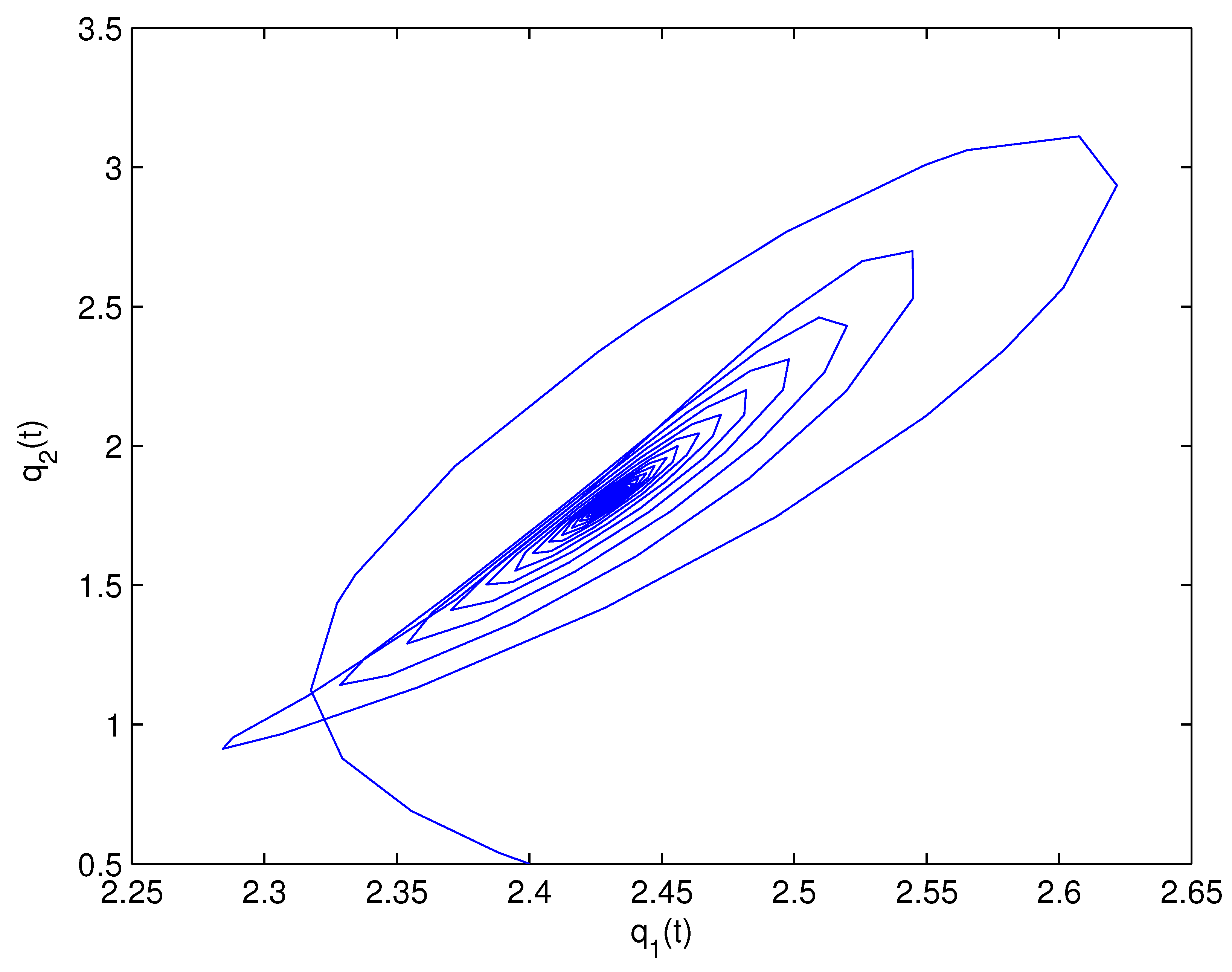
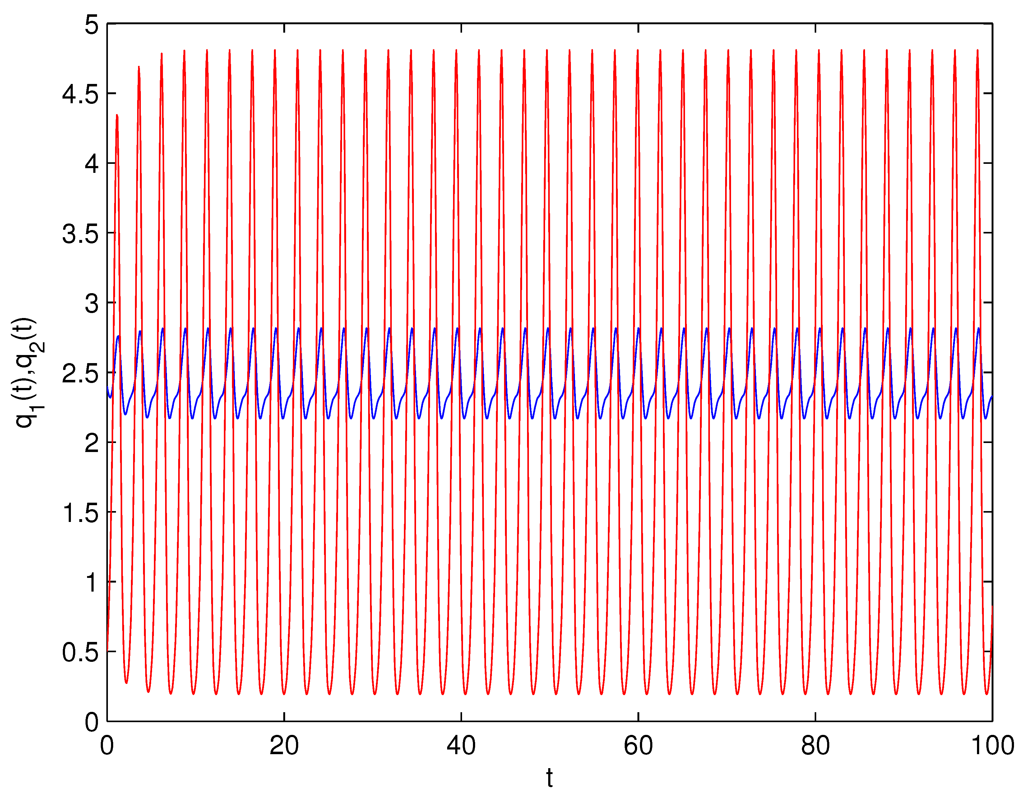
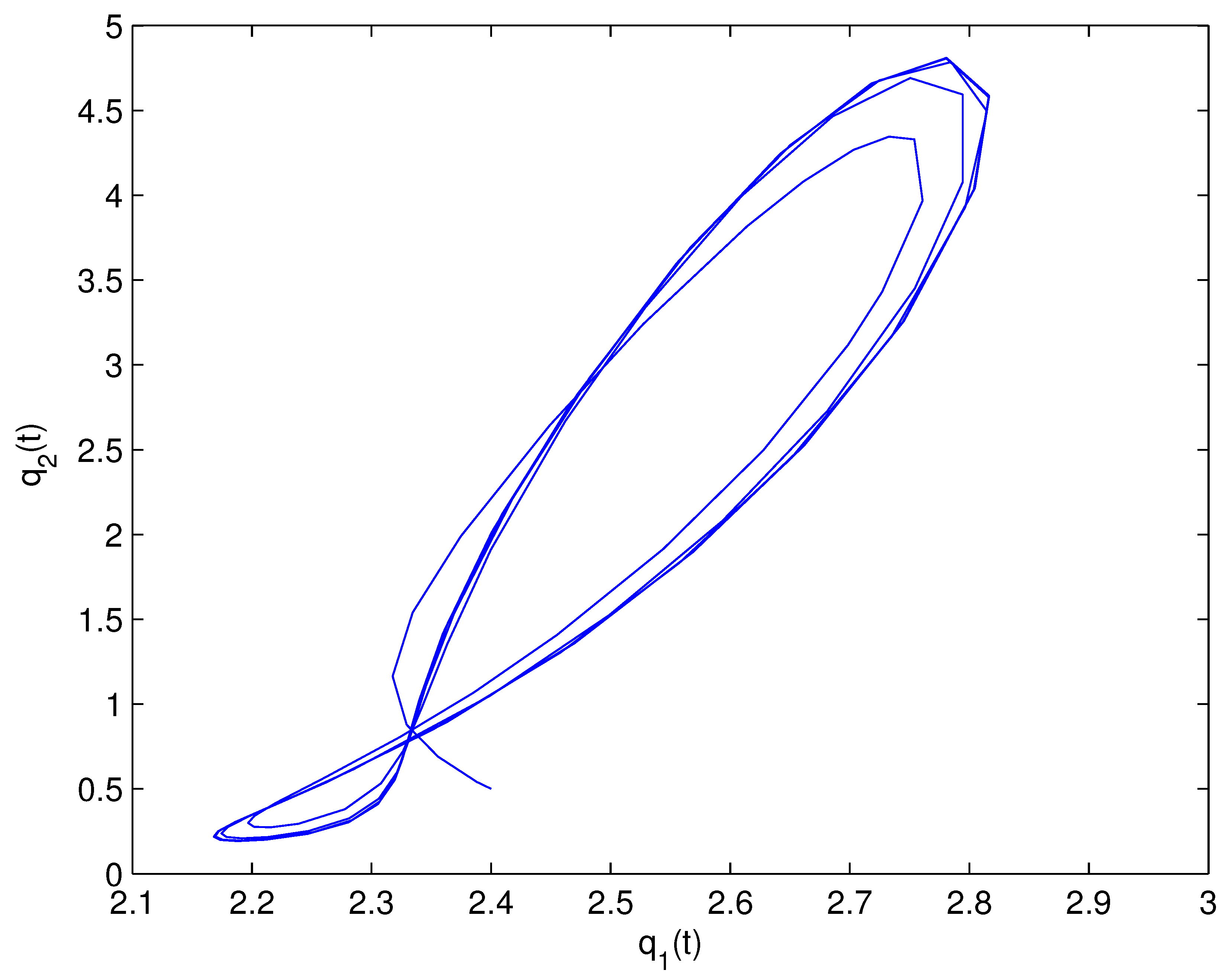
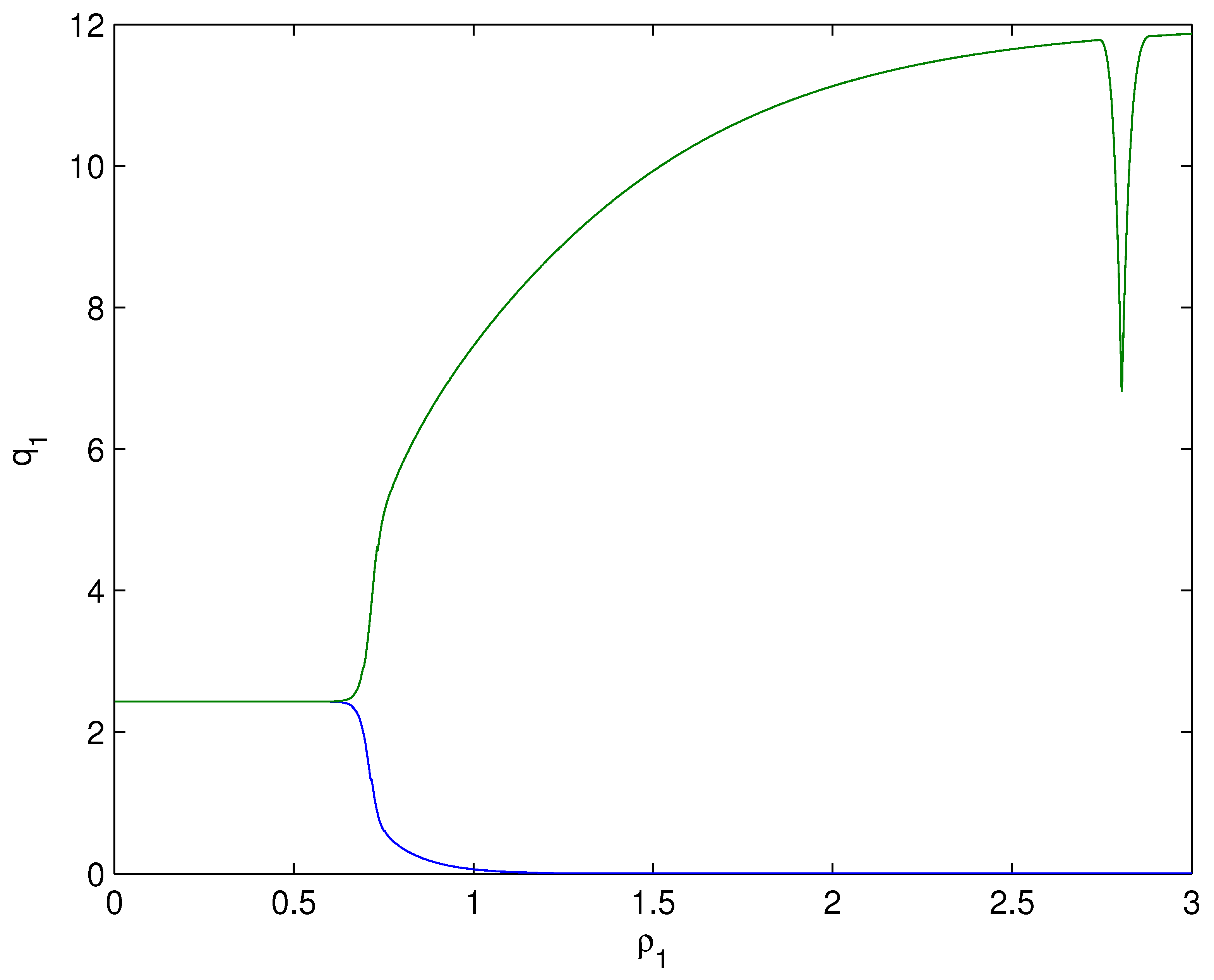
where μ 1 = 0.5 , μ 2 = 0.5 , α 1 = 6 , α 2 = 5 , β 1 = 1.5 , β 2 = 1.8 , ϖ = 0.2 , δ 1 = 0.3 , δ 2 = 0.4 , γ 1 = 0.5 , γ 2 = 0.3 , a n d ϱ = 0.91 . Clearly, δ 1 δ 2 = 0.3 × 0.4 = 0.12 and 4 β 1 β 2 = 4 × 1.5 × 1.8 = 10.8 . Then, δ 1 δ 2 < 4 β 1 β 2 . So ( N 1 ) holds. Thus, system (99) has a unique unique positive equilibrium point Q 4 ( 2.4309 , 1.8090 ) . Next, we will check the assumptions of Theorems 3–7. By virtue of computer software, we can verify that all the assumptions ( N 2 ) ( N 12 ) are fulfilled. Thus, the conclusions of Theorems 3–7 hold true. In order to display the simulation results in Theorems 3–7, we are to select different delay values.
(1)
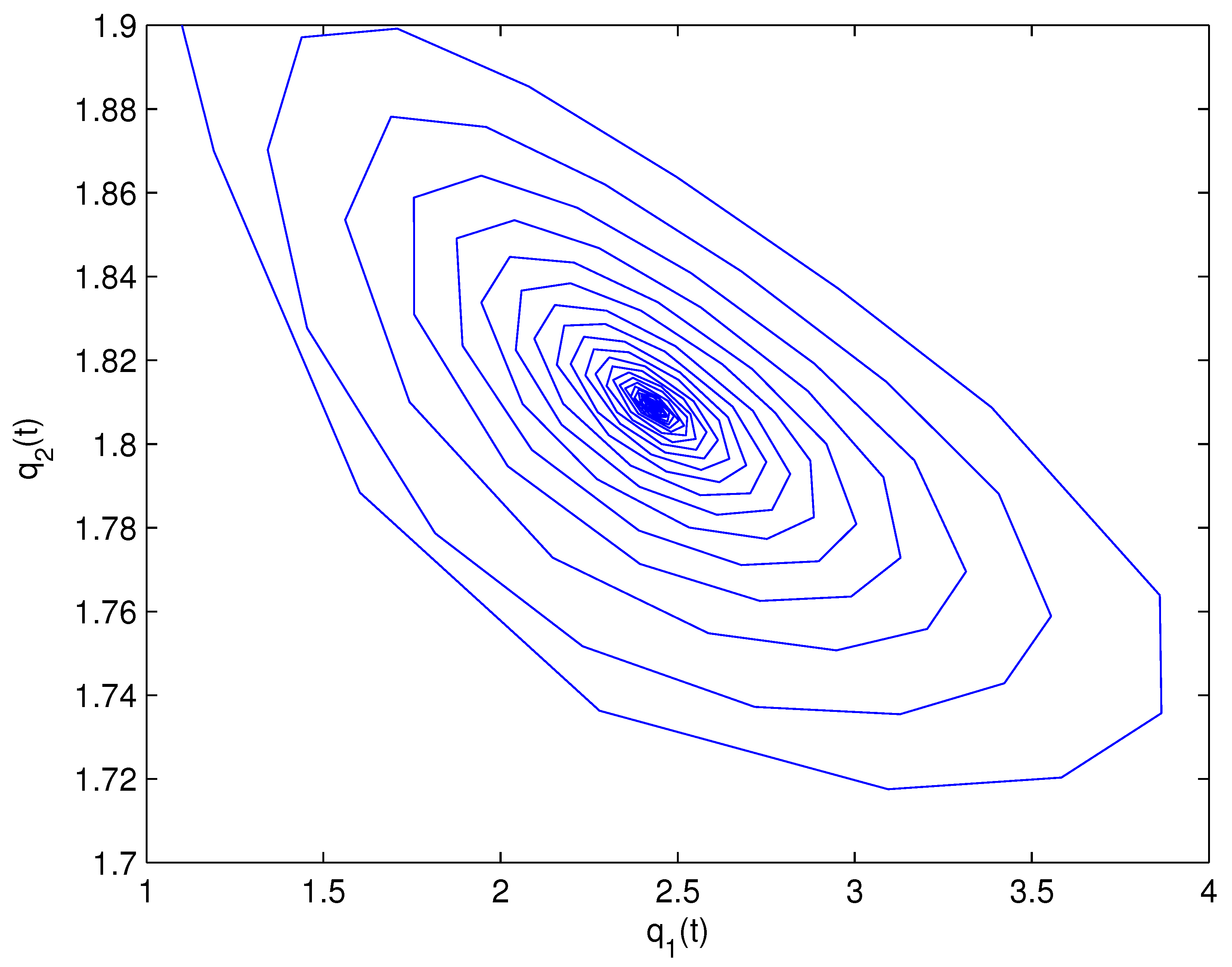
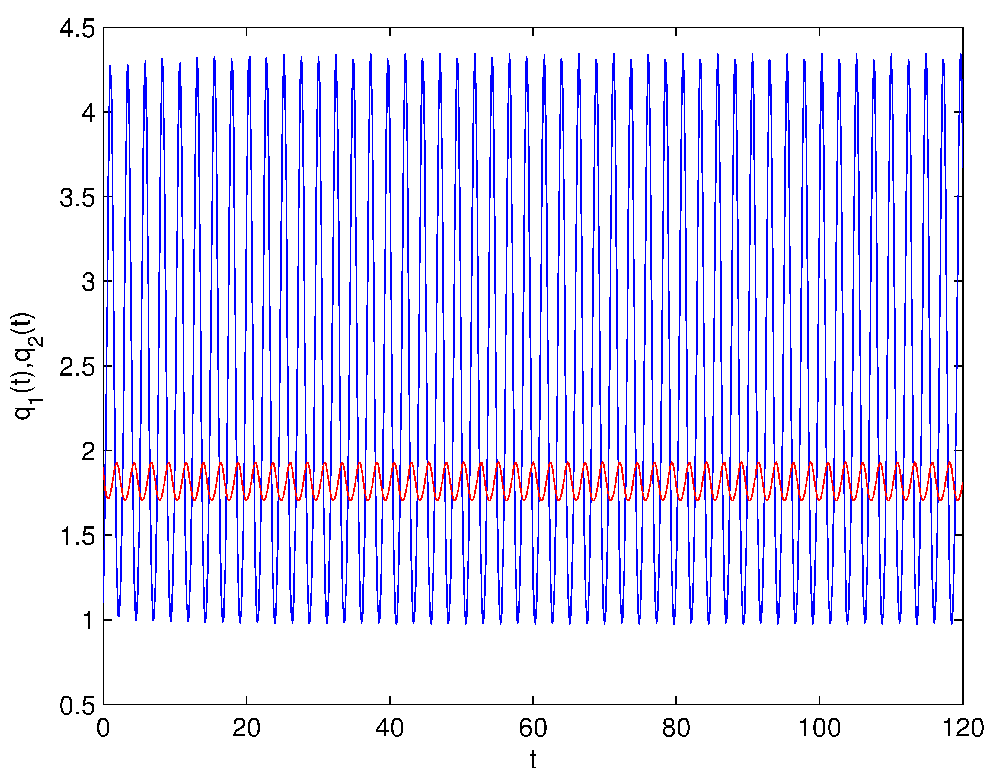
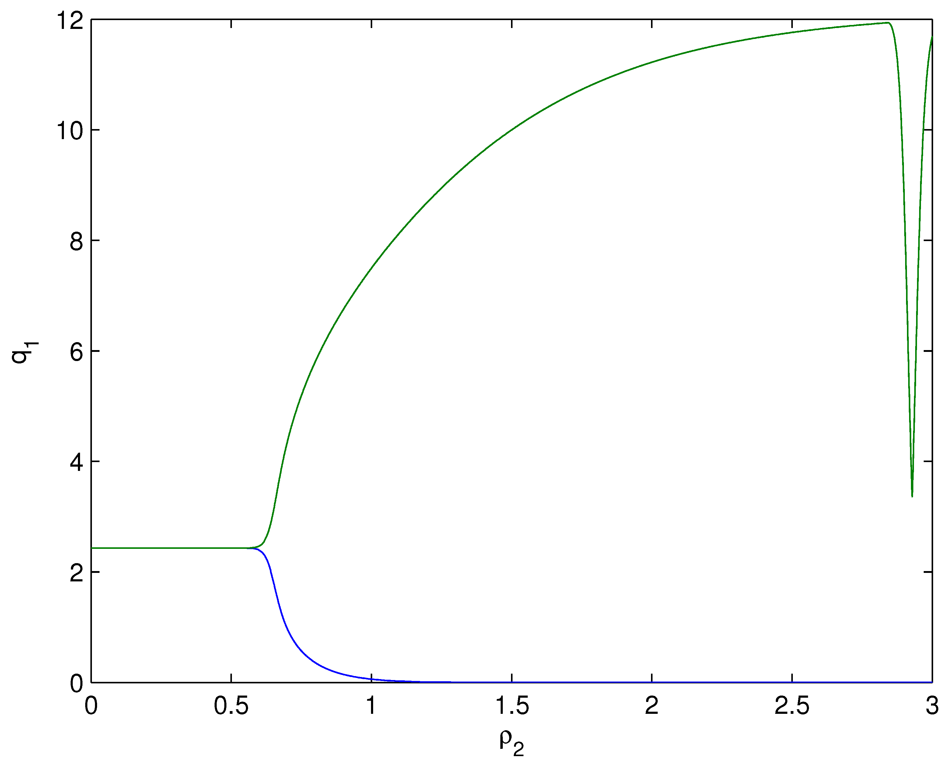
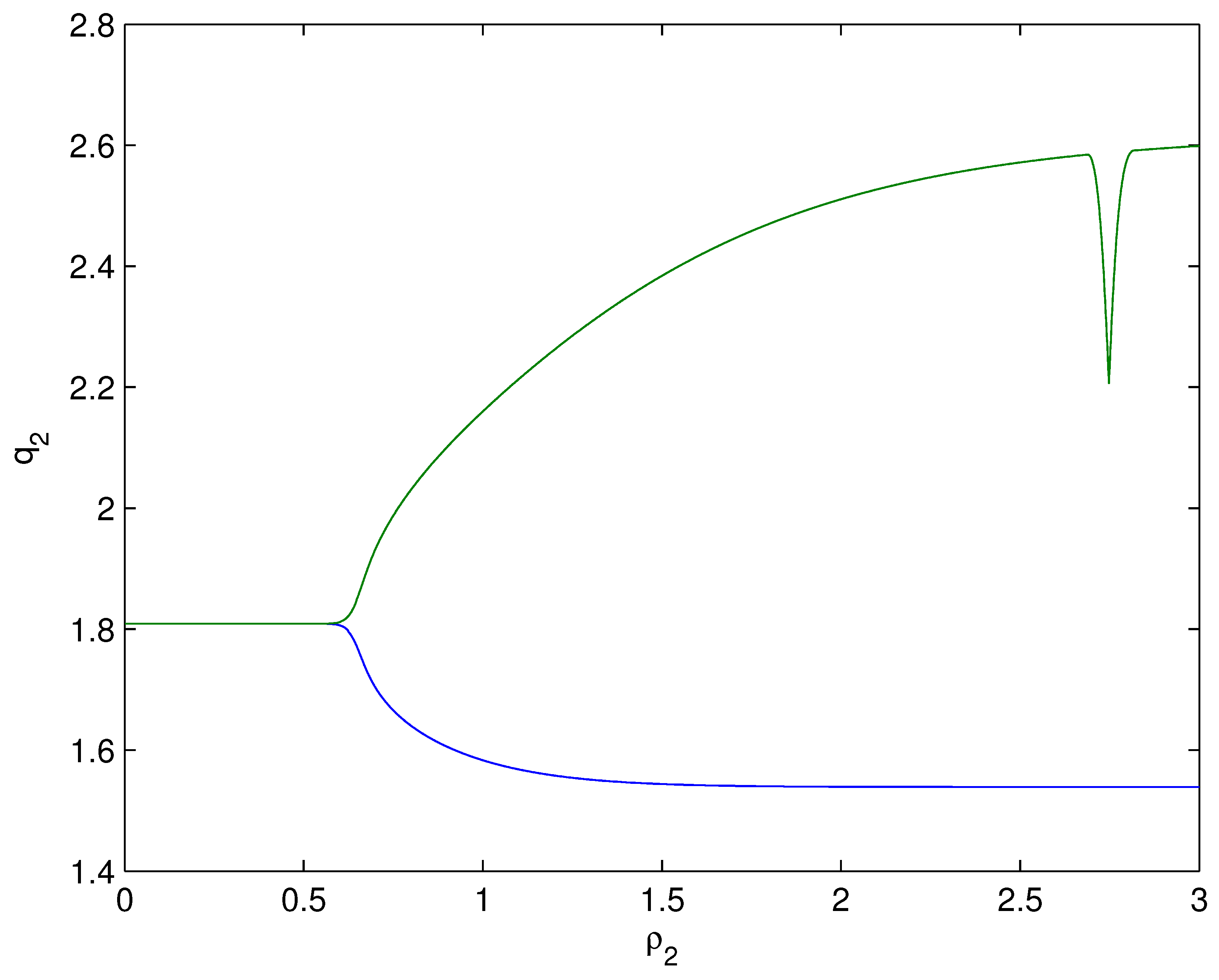
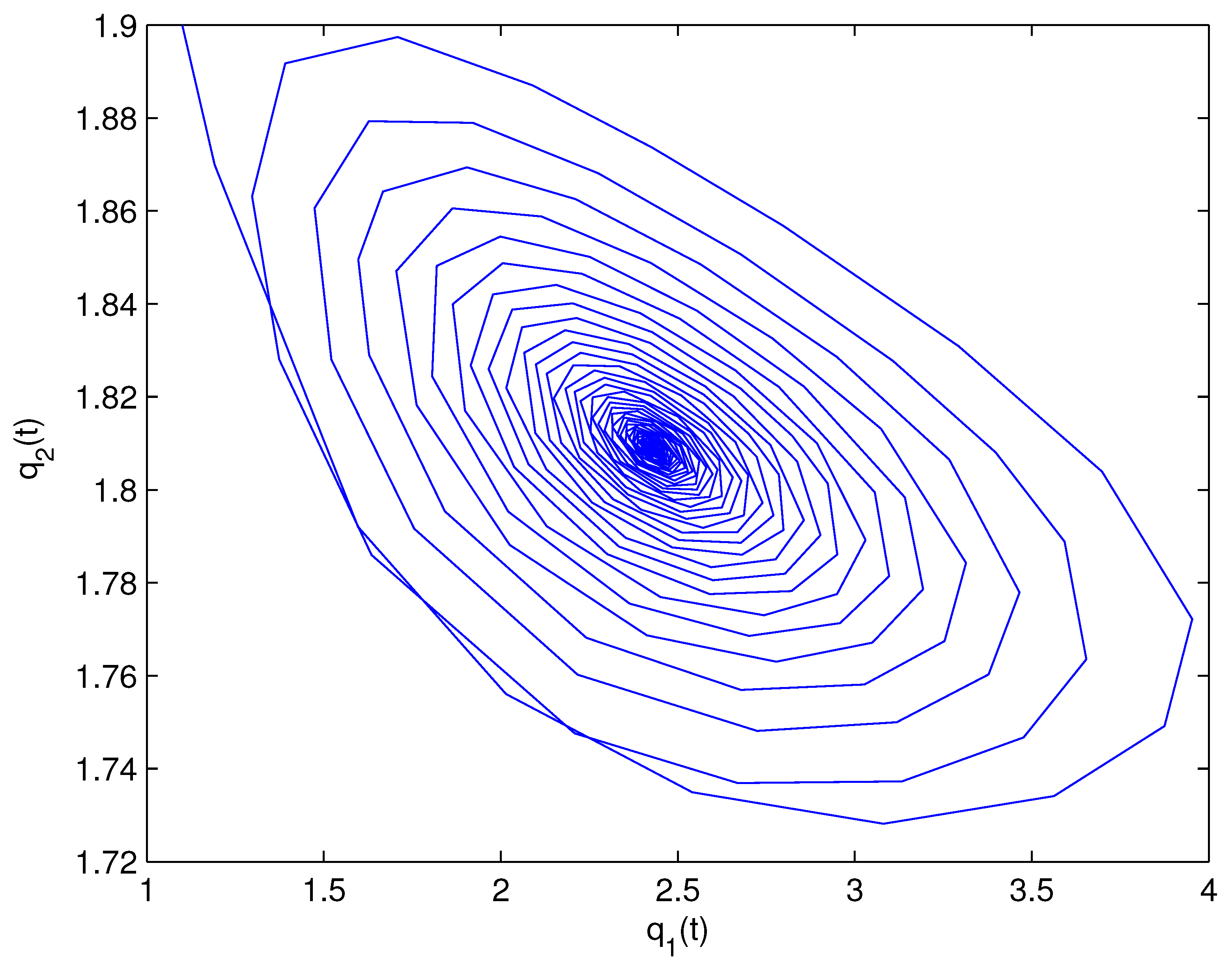
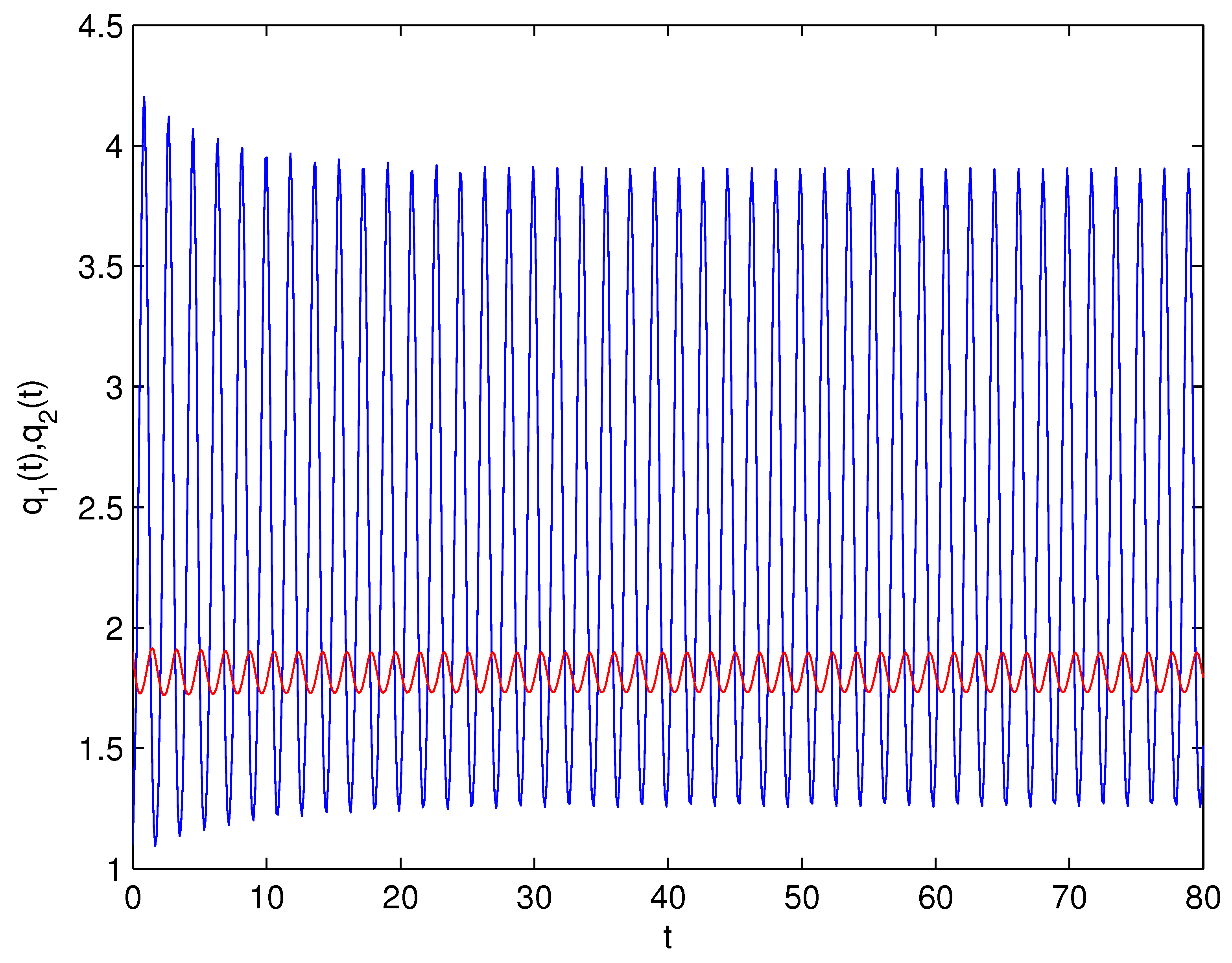
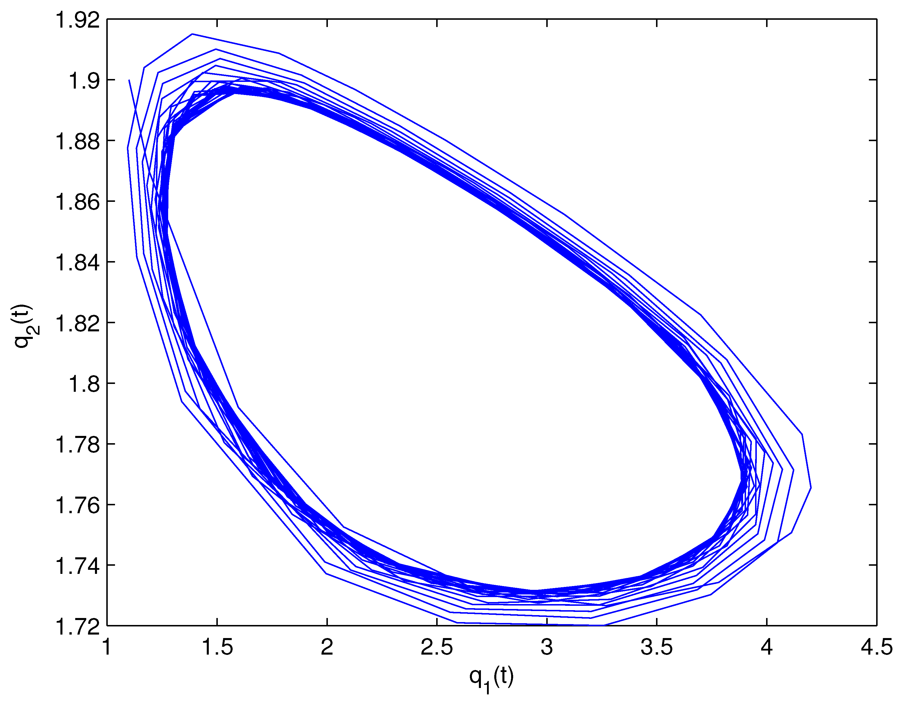
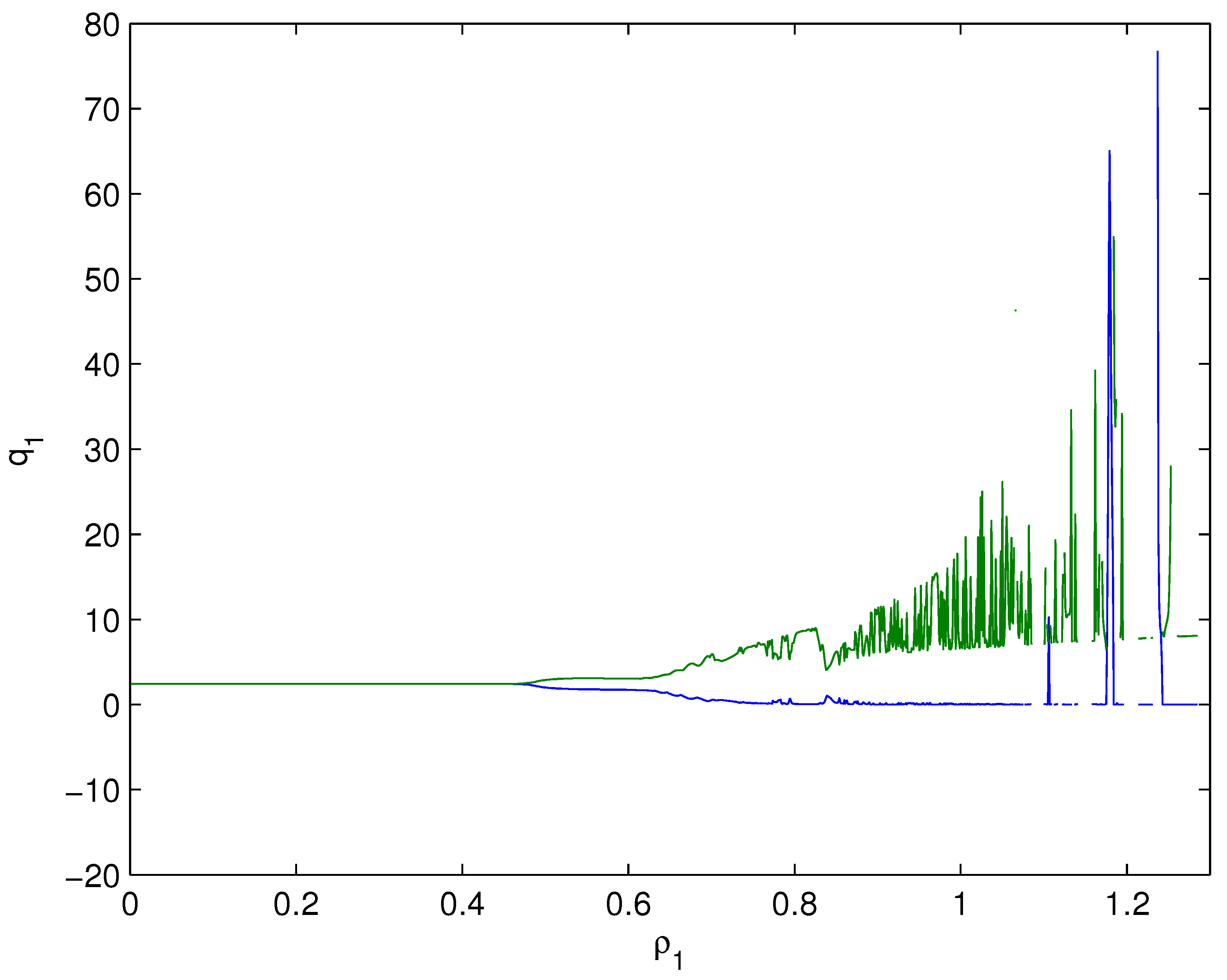
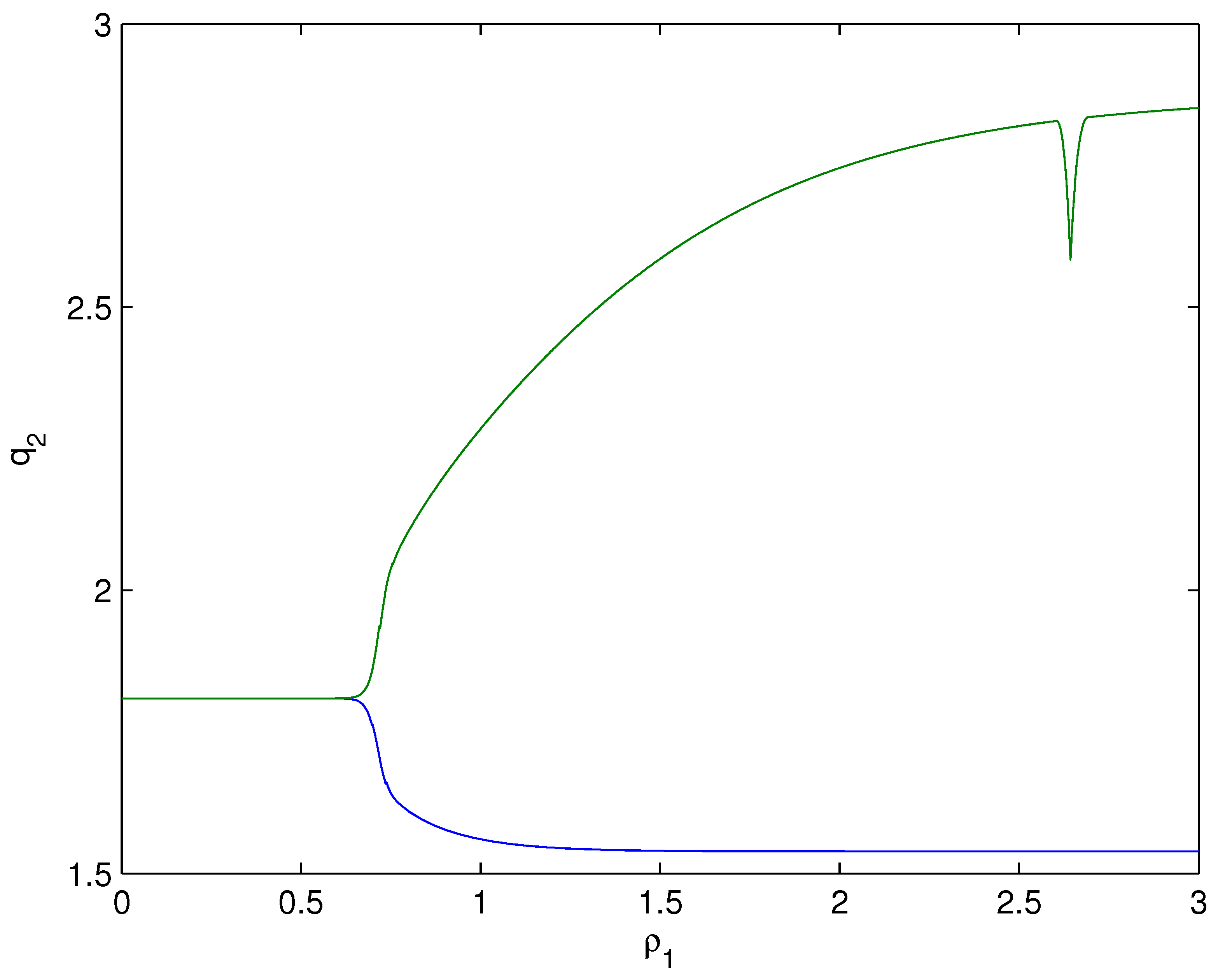
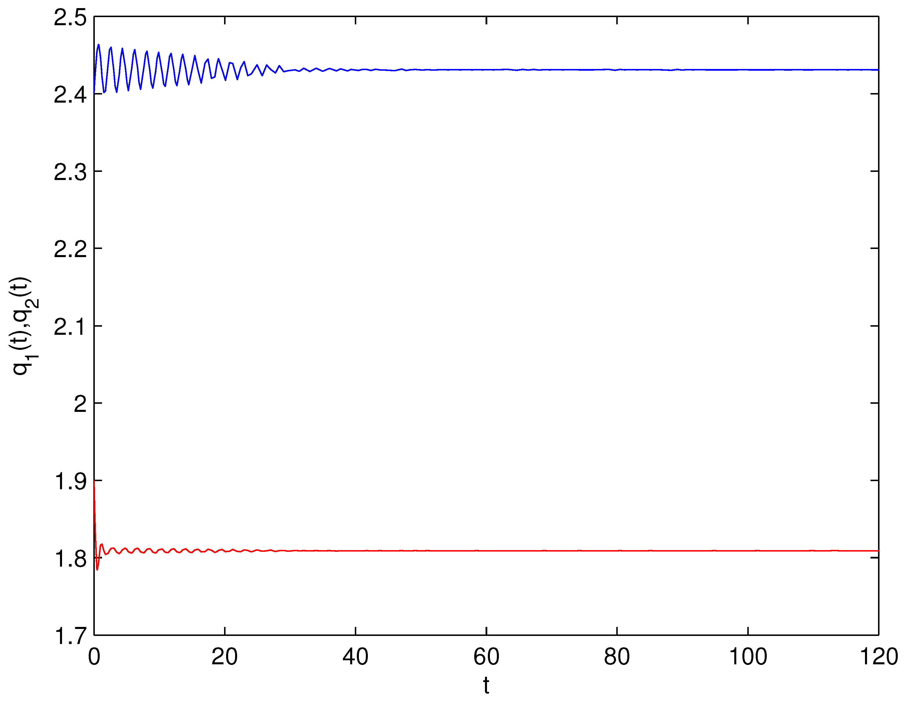
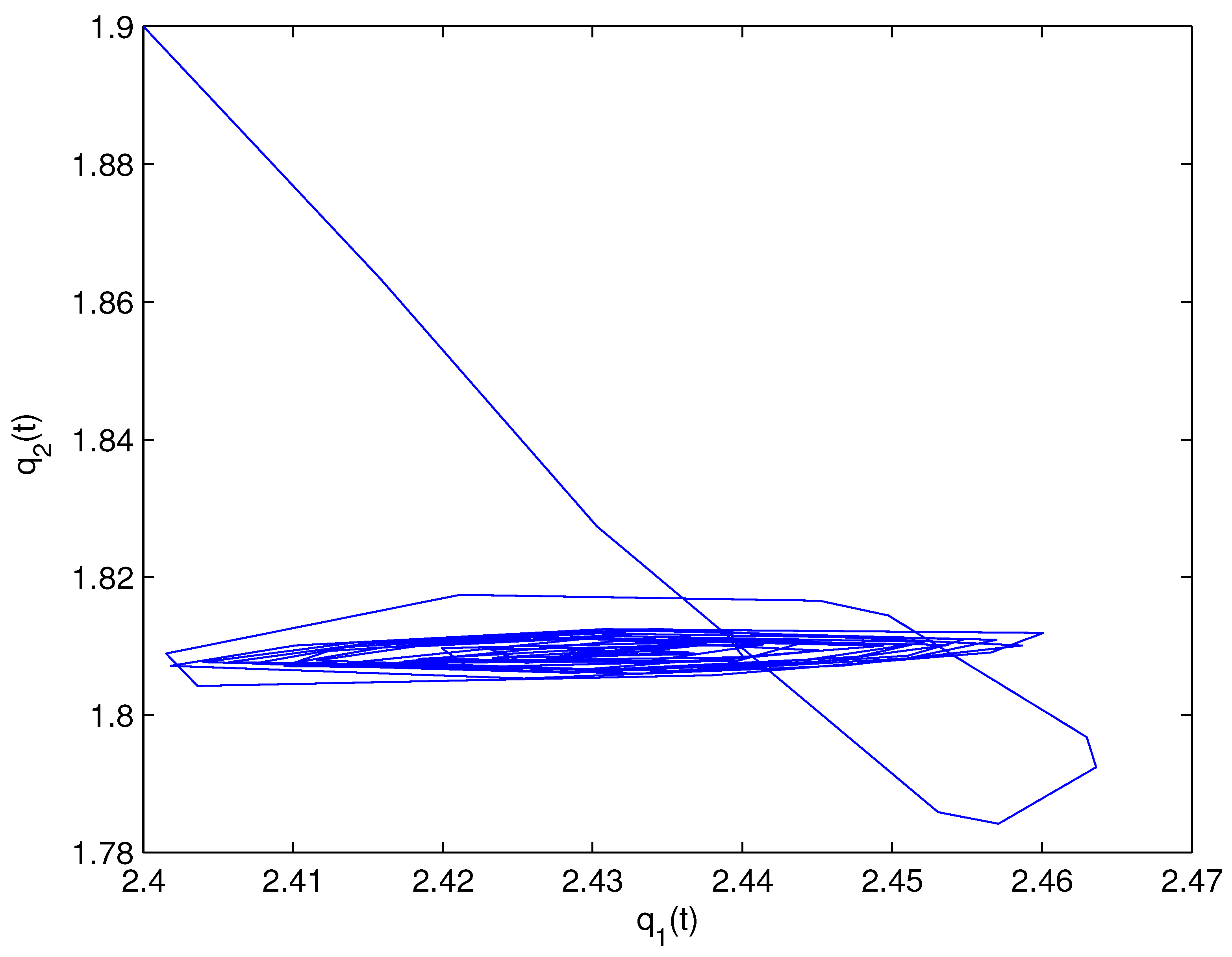
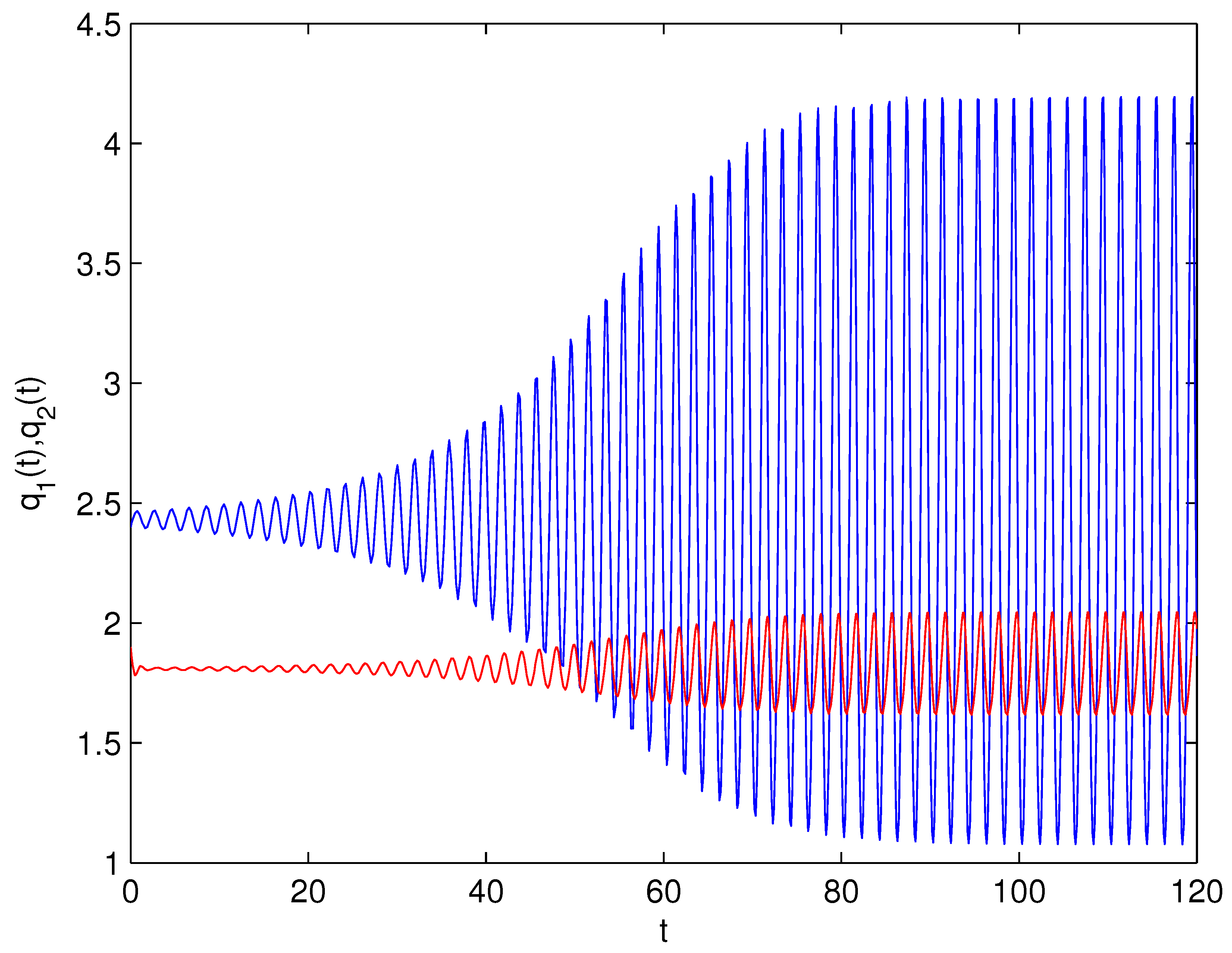
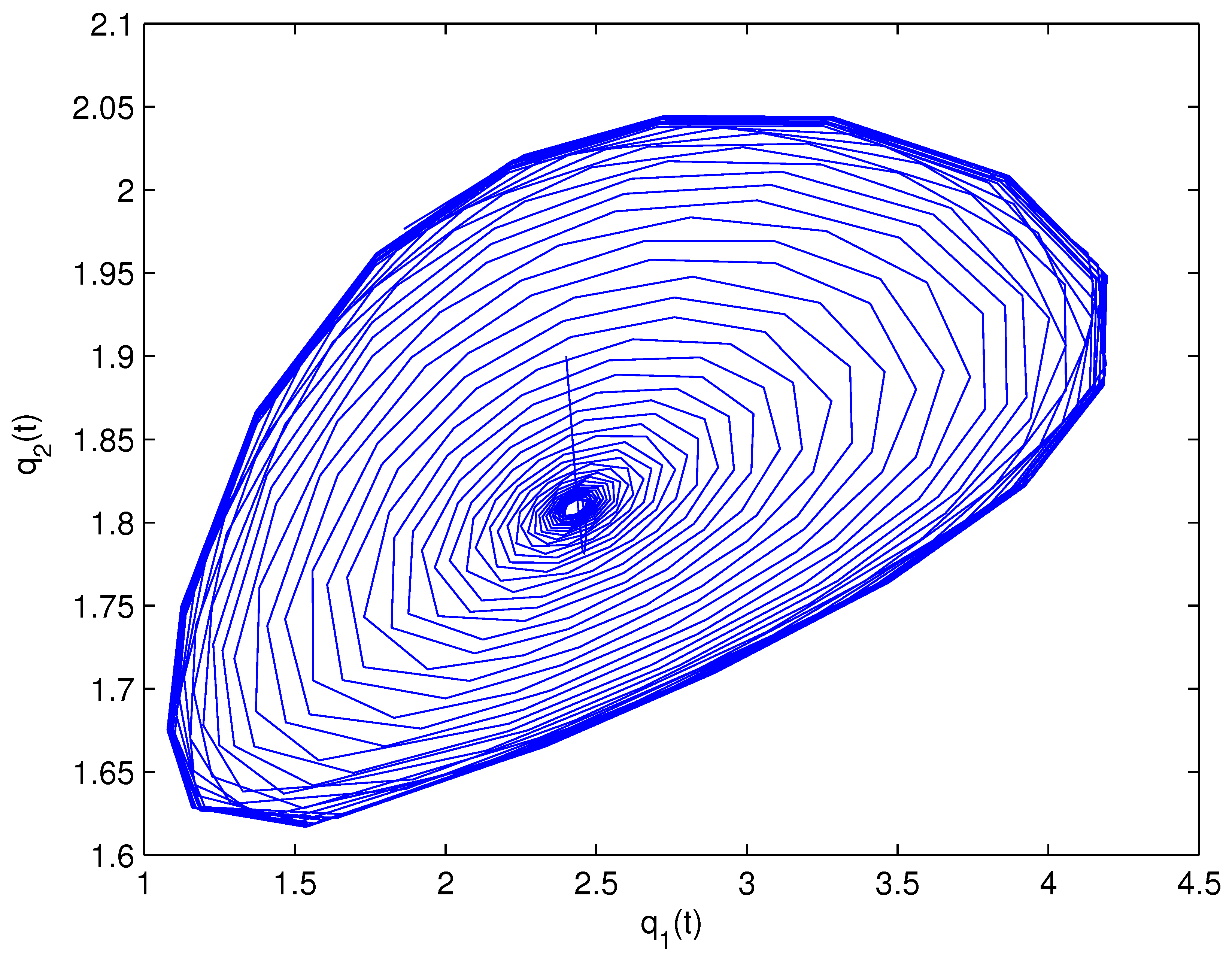
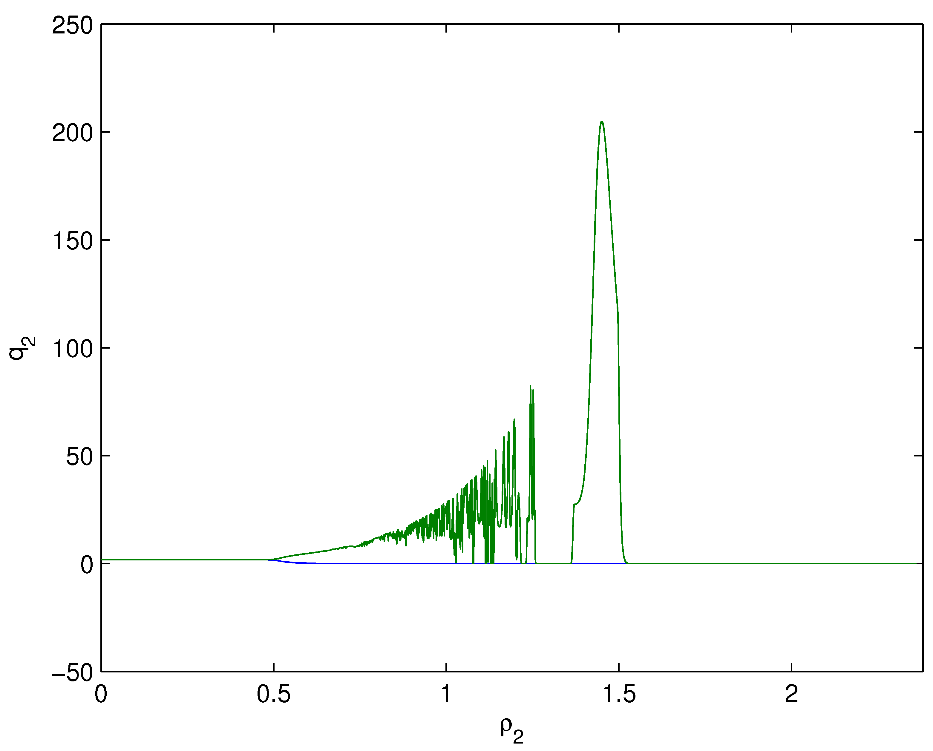
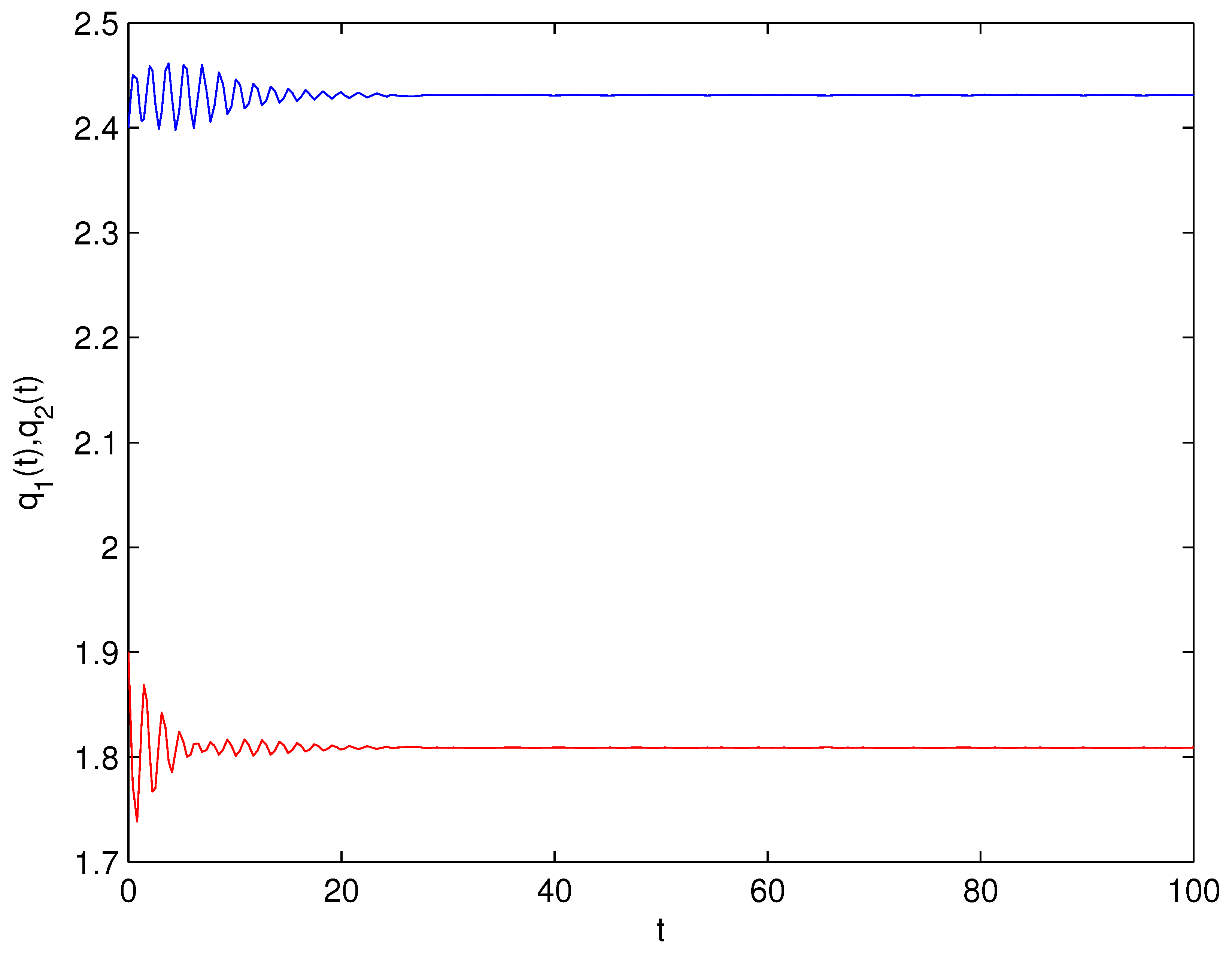
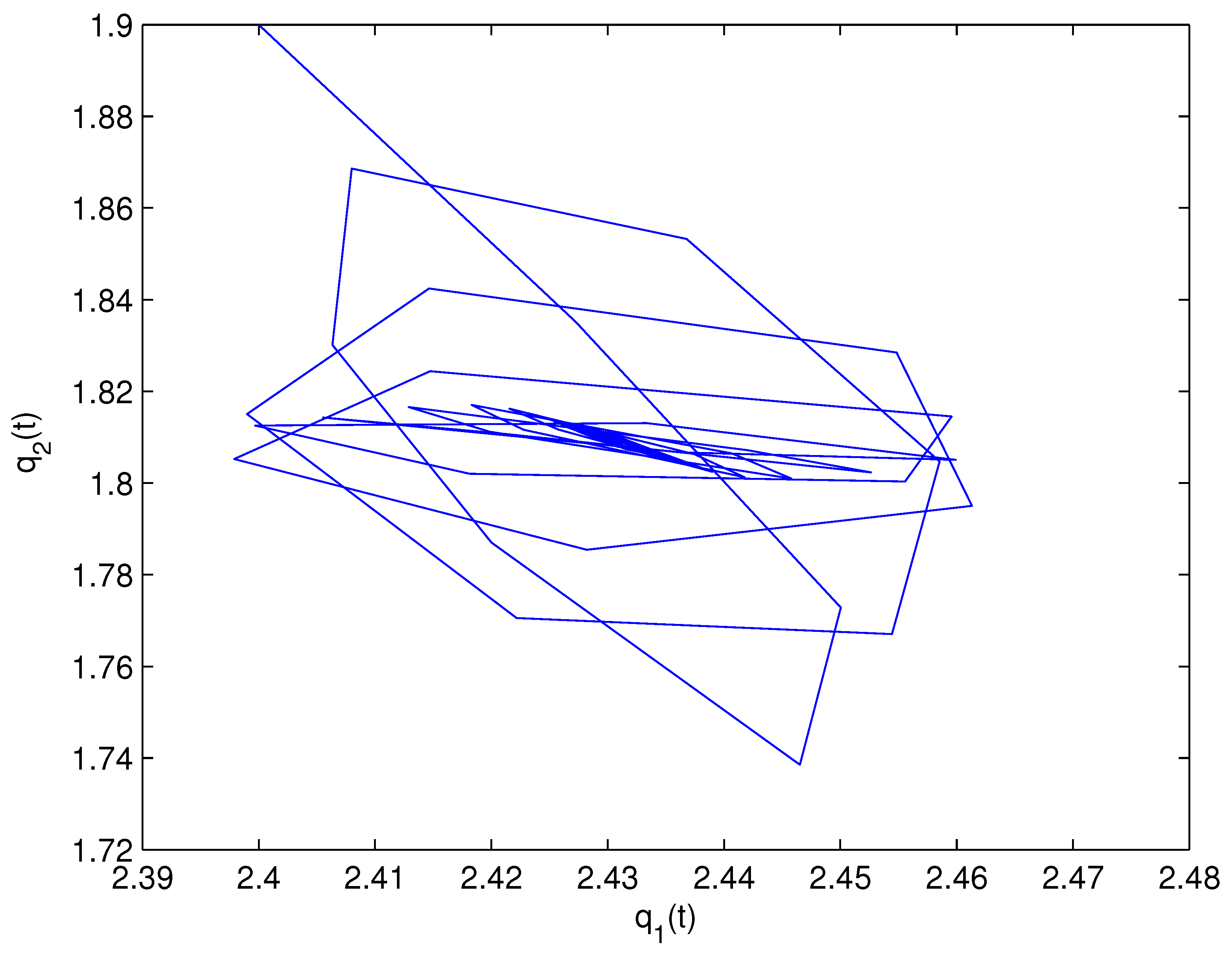
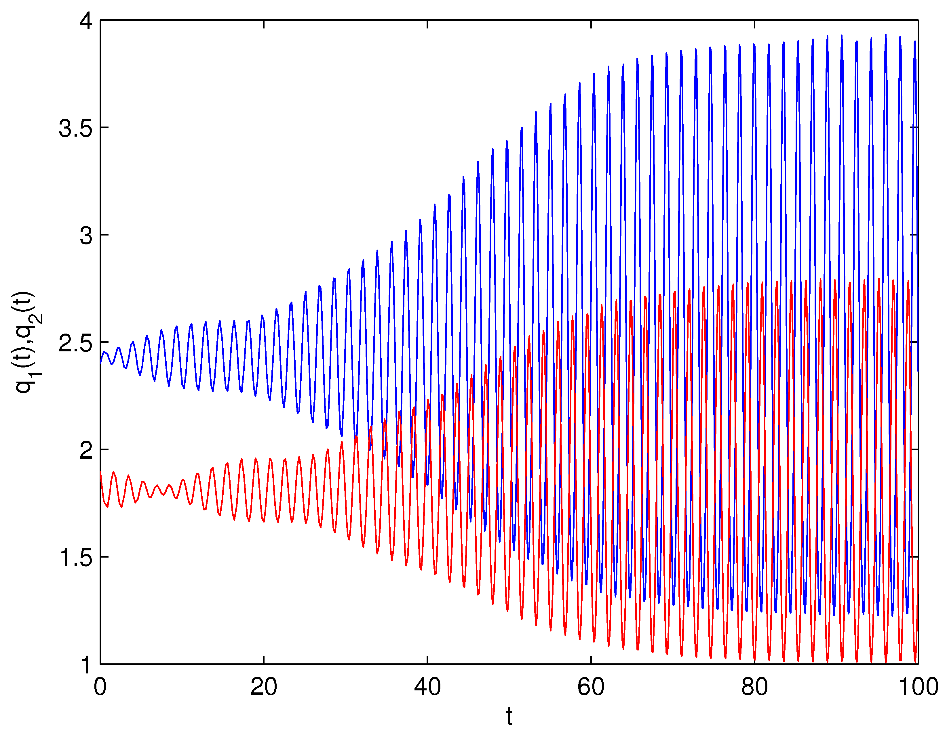
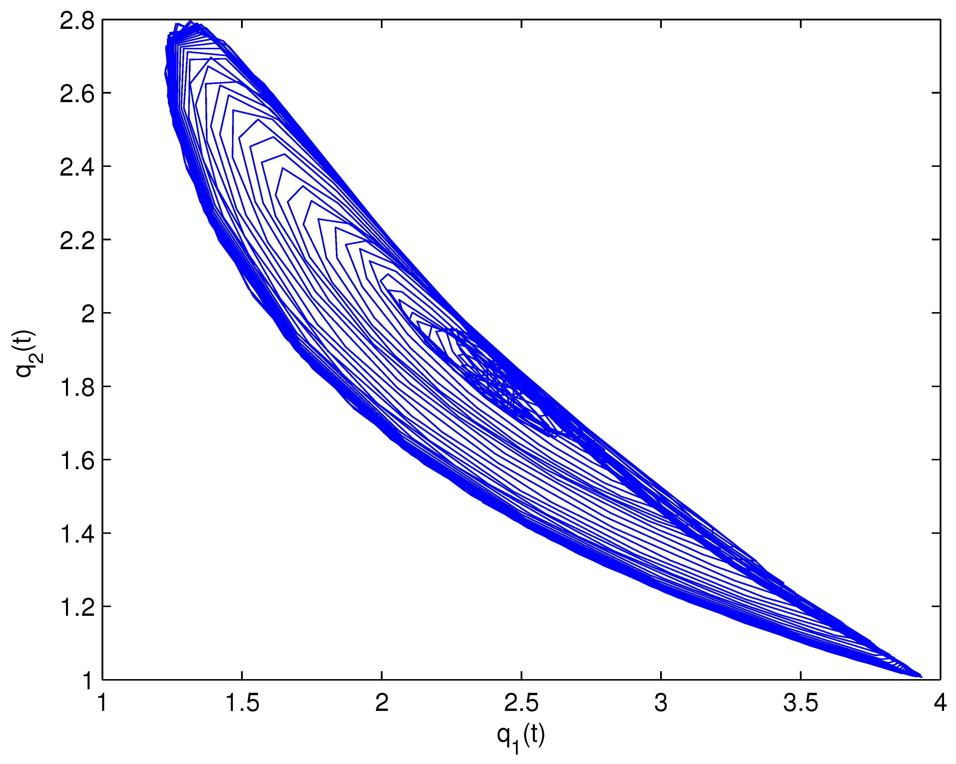
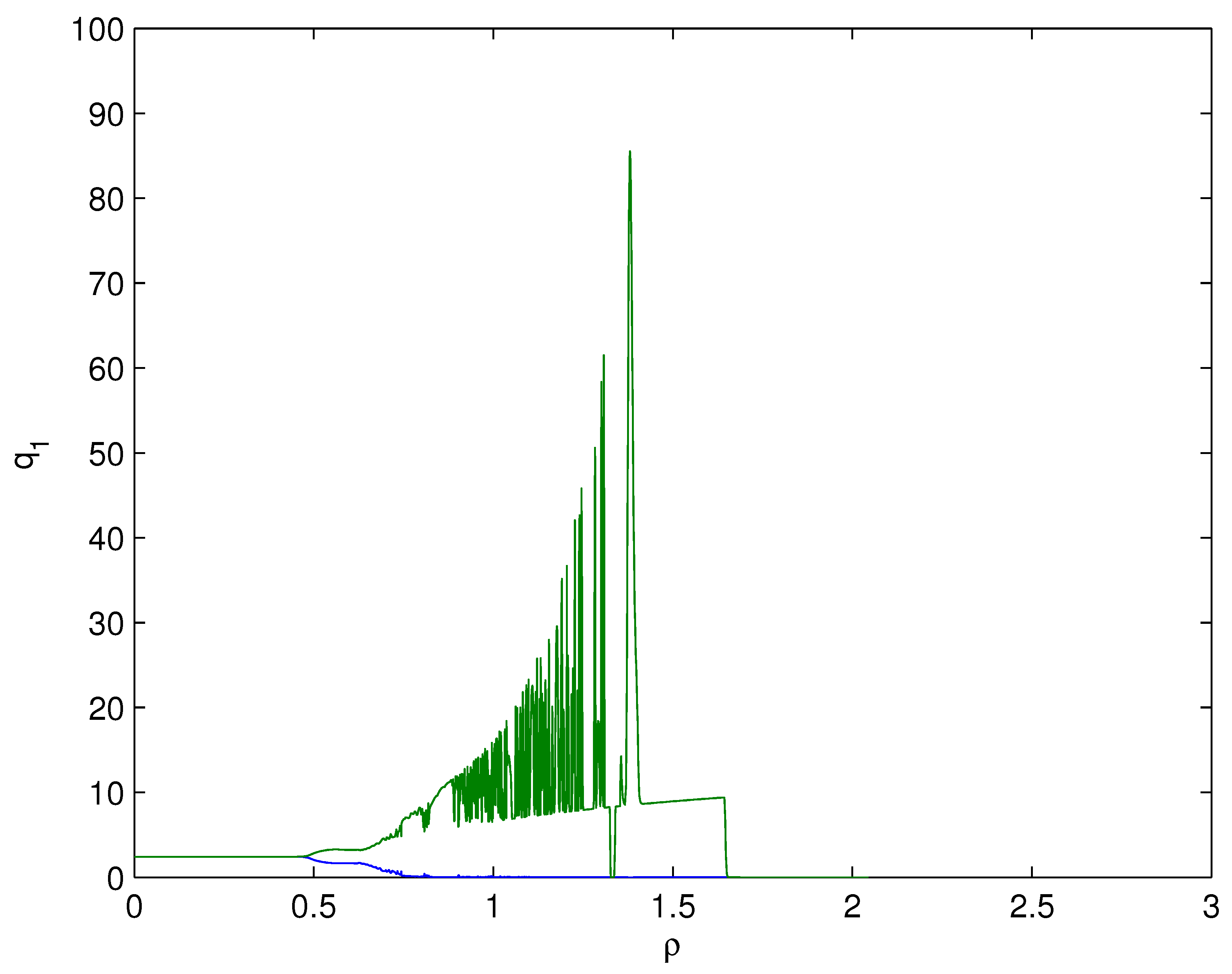
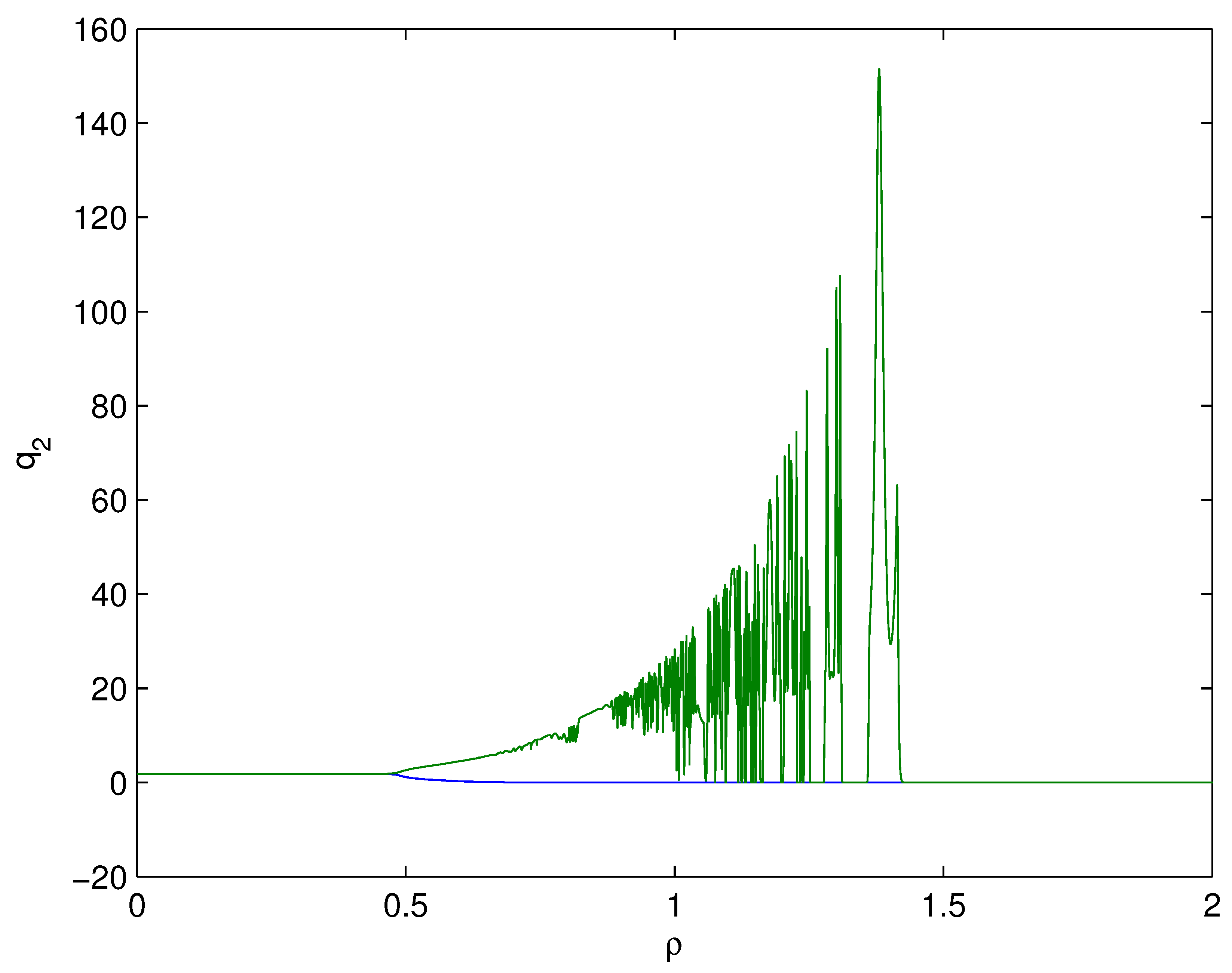
For Theorem 3, fix ρ 1 = 0 . We obtain ρ 20 0.59 and θ 0 = 2.3905 . Let ρ 2 = 0.55 and ρ 2 = 0.7 . The numerical simulation plots are presented in Figure 1, Figure 2, Figure 3, Figure 4, Figure 5 and Figure 6. Figure 1 shows the time history plots of system (99) with ρ 1 = 0 , ρ 2 = 0.55 < ρ 20 0.59 . Figure 2 shows the phase plot of system (99) with ρ 1 = 0 , ρ 2 = 0.55 < ρ 20 0.59 . From Figure 1 and Figure 2, we can see the locally asymptotically stable level of the positive equilibrium point Q 4 ( 2.4309 , 1.8090 ) of system (99), which indicates that the price of the company I will tend to 2.4309 and the price of the company II will tend to 1.8090 . Figure 3 shows the time history plots of system (99) with ρ 1 = 0 , ρ 2 = 0.7 > ρ 20 0.59 . Figure 4 shows the phase plot of system (99) with ρ 1 = 0 , ρ 2 = 0.7 > ρ 20 0.59 . From Figure 3 and Figure 4, we can see the onset of Hopf bifurcation near the positive equilibrium point Q 4 ( 2.4309 , 1.8090 ) of system (99), which shows that the price of the company I will keep periodic vibration around 2.4309 and the price of the company II will keep periodic vibration around 1.8090 . Figure 5 shows the bifurcation plot of system (99) with respect to t and q 1 under ρ 1 = 0 . Figure 6 shows the bifurcation plot of system (99) with respect to t and q 2 under ρ 1 = 0 . From Figure 5 and Figure 6, we can see the bifurcation value ρ 20 0.59 .
(2)
For Theorem 4, fix ρ 2 = 0 . We obtain ρ 10 0.48 , η 0 = 1.8704 . Let ρ 1 = 0.44 and ρ 1 = 0.56 . The numerical simulation plots are presented in Figure 7, Figure 8, Figure 9, Figure 10, Figure 11 and Figure 12. Figure 7 shows the time history plots of system (99) with ρ 2 = 0 , ρ 1 = 0.44 < ρ 10 0.48 . Figure 8 shows the phase plot of system (99) with ρ 2 = 0 , ρ 1 = 0.44 < ρ 10 0.48 . From Figure 7 and Figure 8, we can see the locally asymptotically stable level of the positive equilibrium point Q 4 ( 2.4309 , 1.8090 ) of system (99), which indicates that the price of the company I will tend to 2.4309 and the price of the company II will tend to 1.8090 . Figure 9 shows the time history plots of system (99) with ρ 2 = 0 , ρ 1 = 0.56 > ρ 10 0.48 . Figure 10 shows the phase plot of system (99) with ρ 2 = 0 , ρ 1 = 0.56 > ρ 10 0.48 . From Figure 9 and Figure 10, we can see the onset of Hopf bifurcation near the positive equilibrium point Q 4 ( 2.4309 , 1.8090 ) of system (99), which shows that the price of the company I will keep periodic vibration around 2.4309 and the price of the company II will keep periodic vibration around 1.8090 . Figure 11 shows the bifurcation plot of system (99) with respect to t and q 1 under ρ 2 = 0 . Figure 12 shows the bifurcation plot of system (99) with respect to t and q 2 ρ 2 = 0 . From Figure 11 and Figure 12, we can see the bifurcation value ρ 10 0.48 .
(3)
For Theorem 5, fix ρ 2 = 0.5 . We obtain ρ 1 0.61 , ζ 0 = 2.0933 . Let ρ 1 = 0.55 and ρ 1 = 0.67 . The numerical simulation plots are presented in Figure 13, Figure 14, Figure 15, Figure 16, Figure 17 and Figure 18. Figure 13 shows the time history plots of system (99) with ρ 2 = 0.5 , ρ 1 = 0.55 < ρ 1 0.61 . Figure 14 shows the phase plot of system (99) with ρ 2 = 0.5 , ρ 1 = 0.55 < ρ 1 0.61 . From Figure 13 and Figure 14, we can see the locally asymptotically stable level of the positive equilibrium point Q 4 ( 2.4309 , 1.8090 ) of system (99), which indicates that the price of the company I will tend to 2.4309 and the price of the company II will tend to 1.8090 . Figure 15 shows the time history plots of system (99) with ρ 2 = 0.5 , ρ 1 = 0.67 > ρ 1 0.61 . Figure 16 shows the phase plot of system (99) with ρ 2 = 0.5 , ρ 1 = 0.67 > ρ 1 0.61 . From Figure 15 and Figure 16, we can see the onset of Hopf bifurcation near the positive equilibrium point Q 4 ( 2.4309 , 1.8090 ) of system (99), which shows that the price of the company I will keep periodic vibration around 2.4309 and the price of the company II will keep periodic vibration around 1.8090 . Figure 17 shows the bifurcation plot of system (99) with respect to t and q 1 under ρ 2 = 0.5 . Figure 18 shows the bifurcation plot of system (99) with respect to t and q 2 under ρ 2 = 0.5 . From Figure 17 and Figure 18, we can see the bifurcation value ρ 1 0.61 .
(4)
For Theorem 6, fix ρ 1 = 0.4 . We obtain ρ 2 0.50 , ϕ 0 = 2.0933 . Let ρ 2 = 0.45 and ρ 2 = 0.62 . The numerical simulation plots are presented in Figure 19, Figure 20, Figure 21, Figure 22, Figure 23 and Figure 24. Figure 19 shows the time history plots of system (99) with ρ 1 = 0.4 , ρ 2 = 0.45 < ρ 2 0.50 . Figure 20 shows the phase plot of system (99) with ρ 1 = 0.4 , ρ 2 = 0.45 < ρ 2 0.50 . From Figure 19 and Figure 20, we can see the locally asymptotically stable level of the positive equilibrium point Q 4 ( 2.4309 , 1.8090 ) of system (99), which indicates that the price of the company I will tend to 2.4309 and the price of the company II will tend to 1.8090 . Figure 21 shows the time history plots of system (99) with ρ 1 = 0.4 , ρ 2 = 0.62 > ρ 1 0.50 . Figure 22 shows the phase plot of system (99) with ρ 1 = 0.4 , ρ 2 = 0.62 > ρ 1 0.50 . From Figure 21 and Figure 22, we can see the onset of Hopf bifurcation near the positive equilibrium point Q 4 ( 2.4309 , 1.8090 ) of system (99), which shows that the price of the company I will keep periodic vibration around 2.4309 and the price of the company II will keep periodic vibration around 1.8090 . Figure 23 shows the bifurcation plot of system (99) with respect to t and q 1 under ρ 1 = 0.4 . Figure 24 shows the bifurcation plot of system (99) with respect to t and q 2 under ρ 1 = 0.4 . From Figure 23 and Figure 24, we can see the bifurcation value ρ 2 0.50 .
(5)
For Theorem 7, let ρ 1 = ρ 2 = ρ . We obtain ρ 0 0.49 , ψ 0 = 2.3905 . Let ρ = 0.42 and ρ = 0.53 . The numerical simulation plots are presented in Figure 25, Figure 26, Figure 27, Figure 28, Figure 29 and Figure 30. Figure 25 shows the time history plots of system (99) with ρ = 0.42 < ρ 0 0.49 . Figure 26 shows the phase plot of system (99) with ρ = 0.42 < ρ 0 0.49 . From Figure 25 and Figure 26, we can see the locally asymptotically stable level of the positive equilibrium point Q 4 ( 2.4309 , 1.8090 ) of system (99), which shows that the price of the company I will keep periodic vibration around 2.4309 and the price of the company II will keep periodic vibration around 1.8090 . Figure 27 shows the time history plots of system (99) with ρ = 0.53 > ρ 0 0.49 . Figure 28 shows the phase plot of system (99) with ρ = 0.53 > ρ 0 0.49 . From Figure 27 and Figure 28, we can see the onset of Hopf bifurcation near the positive equilibrium point Q 4 ( 2.4309 , 1.8090 ) of system (99), which shows that the price of the company I will keep periodic vibration around 2.4309 and the price of the company II will keep periodic vibration around 1.8090 . Figure 29 shows the bifurcation plot of system (99) with respect to t and q 1 under ρ 1 = ρ 2 = ρ . Figure 30 shows the bifurcation plot of system (99) with respect to t and q 2 under ρ 1 = ρ 2 = ρ . From Figure 29 and Figure 30, we can see the bifurcation value ρ 0 0.49 .

7. Conclusions

We all know that the competition among different firms has become fierce in contemporary society. In particular, the price of the products of firms is a very vital factor that affects the market and attracts consumers. Thus, the exploration on the price of the products of firms has attracted great interest from many scholars. In this article, we set up a novel fractional-order Bertrand duopoly game model incorporating both nonidentical time delays. The rich dynamical behavior including the existence and uniqueness, non-negativeness, boundedness of solution, local stability, Hopf bifurcation, and globally asymptotical stability of the established fractional-order Bertrand duopoly game model incorporating both nonidentical time delays has been sufficiently explored. In particular, five sufficient conditions to ensure the stability and the onset of Hopf bifurcation of the fractional-order Bertrand duopoly game model are successfully built. These delay cases includes the following situations: (1) ρ 1 = 0 , ρ 2 > 0 ; (2) ρ 2 = 0 , ρ 1 > 0 ; (3) ρ 2 > 0 and ρ 2 [ 0 , ρ 20 ) , ρ 1 > 0 ; (4) ρ 1 > 0 and ρ 1 [ 0 , ρ 10 ) , ρ 2 > 0 ; (5) ρ 1 = ρ 2 = ρ . The influence of different types of time delays on the stability and the creation of Hopf bifurcation of the established fractional-order Bertrand duopoly game model has been fully revealed. The derived research results have important theoretical guiding significance in managing and operating firms. Furthermore, the research idea and mathematical analysis skills can be also utilized to explore bifurcation issue of abundant other multi-delayed fractional dynamical models existing in numerous disciplines. In the near future, we will deal with the chaos control issue and the effect of fractional order on chaos for the fractional-order Bertrand duopoly game model.

Author Contributions

Methodology, Y.L., P.L., C.X. and Y.X.; Software, Y.L. and C.X.; Validation, Y.X.; Formal analysis, Y.L., P.L. and C.X.; Investigation, P.L. and Y.X.; Data curation, Y.L.; Writing—original draft, Y.L., P.L. and C.X.; Writing—review & editing, Y.L., P.L., C.X. and Y.X. All authors have read and agreed to the published version of the manuscript.

Funding

This work is supported by National Natural Science Foundation of China (No. 12261015, No. 62062018), Project of High-level Innovative Talents of Guizhou Province ([2016]5651), Basic research projects of key scientific research projects in Henan province (No. 20ZX001), Key Science and Technology Research Project of Henan Province of China (Grant No. 222102210053) Key Scientific Research Project in Colleges and Universities of Henan Province of China (Grant No. 21A510003), University Science and Technology Top Talents Project of Guizhou Province (KY[2018]047), Foundation of Science and Technology of Guizhou Province ([2019]1051), Guizhou University of Finance and Economics (2018XZD01).

Data Availability Statement

No data were used to support this study.

Conflicts of Interest

The authors declare that they have no conflict of interest.

References

  1. Zhang, J.X.; Da, Q.L.; Wang, Y.H. The dynamics of Bertrand model with bounded rationality. Chaos Solitons Fractals 2009, 39, 2048–2055. [Google Scholar] [CrossRef]
  2. Yu, Y.; Yu, W.S. The stability and duality of dynamic Cournot and Bertrand duopoly model with comprehensive preference. Appl. Math. Comput. 2021, 395, 125852. [Google Scholar] [CrossRef]
  3. Cao, Y.X.; Zhou, W.; Chu, T.; Chang, Y.X. Global dynamics and syschronization in a duopoly game with bounded rationality and consumer surplus. Int. J. Bifurc. Chaos 2019, 29, 1930031. [Google Scholar] [CrossRef]
  4. Baiardi, L.C.; Naimzada, A.K. An oligopoly model with best response and limit rules. Appl. Math. Comput. 2018, 336, 193–205. [Google Scholar]
  5. Zhu, Y.L.; Zhou, W.; Chu, T.; Elsadany, A.A. Complex dynamical behavior and numerical simulation of a Cournot-Bertrand duopoly game with heterogeneous players. Commun. Nonlinear Sci. Numer. Simul. 2021, 101, 105898. [Google Scholar] [CrossRef]
  6. Askar, S.S.; Al-khedhairi, A. Dynamic investigations in a duopoly game with price competition based on relative profit and profit maximization. J. Comput. Appl. Math. 2020, 367, 112464. [Google Scholar] [CrossRef]
  7. Buccella, D.; Fanti, L.; Gori, L. To abate, or not to abate? A strategic approach on green production in Cournot and Bertrand duopolies. Energy Econ. 2021, 96, 105164. [Google Scholar] [CrossRef]
  8. Tolotti, M.; Yepez, J. Hotelling-Bertrand duopoly competition under firm-specific network effects. J. Econ. Behav. Organ. 2020, 176, 105–128. [Google Scholar] [CrossRef]
  9. Askar, S.S. On complex dynamics of Cournot-Bertrand game with asymmetric market information. Appl. Math. Comput. 2021, 393, 125823. [Google Scholar] [CrossRef]
  10. Ahmed, E.; Elsadany, A.A.; Puu, T. On Bertrand duopoly game with differentiated goods. Appl. Math. Comput. 2015, 251, 169–179. [Google Scholar] [CrossRef]
  11. Li, H.; Zhou, W.; Elsadany, A.A.; Chu, T. Stability, multi-stability and instability in Cournot duopoly game with knowledge spillover effects and relative profit maximization. Chaos Solitons Fractals 2021, 146, 110936. [Google Scholar] [CrossRef]
  12. Fanti, L.; Gori, L.; Mammana, C.; Michetti, E. The dynamics of a Bertrand duopoly with differentiated products: Synchronization, intermittency and global dynamics. Chaos Solitons Fractals 2013, 52, 73–86. [Google Scholar] [CrossRef]
  13. Elabbsy, E.M.; Agiza, H.N.; Elsadany, A.A. Analysis of nonlinear triopoly game with heterogeneous players. Comput. Math. Appl. 2009, 57, 488–499. [Google Scholar] [CrossRef]
  14. Ma, J.H.; Sun, L.J.; Hou, S.Q.; Zhan, X.L. Complexity study on the Cournot-Bertrand mixed duopoly game model with market share preference. Chaos 2018, 28, 023101. [Google Scholar] [CrossRef]
  15. Peng, Y.; Lu, Q. Complex dynamics analysis for a duopoly Stackelberg game model with bounded rationality. Appl. Math. Comput. 2015, 271, 259–268. [Google Scholar] [CrossRef]
  16. Ma, J.H.; Li, Q.X. The complex dynamic of Bertrand-Stackelberg pricing models in a risk-averse supply chain. Discret. Dyn. Nat. Soc. 2014, 2014, 749769. [Google Scholar] [CrossRef]
  17. Wang, Y.; Hou, G.S. A duopoly game with heterogeneous green supply chains in optimal price and market stability with consumer green preference. J. Clean. Prod. 2020, 255, 120161. [Google Scholar] [CrossRef]
  18. Safarzadeh, S.; Rasti-Barzoki, M.; Hejazi, S.R.; Piran, M.J. A game theoretic approach for the duopoly pricing of energy-efficient appliances regarding innovation protection and social welfare. Energy 2020, 200, 117517. [Google Scholar] [CrossRef]
  19. Huang, H.; Ke, H.; Wang, L. Equilibrium analysis of pricing competition and cooperation in supply chain with one common manufacturer and duopoly retailers. Int. J. Prod. Econ. 2016, 178, 12–21. [Google Scholar] [CrossRef]
  20. Mukhopadhyay, S.K.; Yue, X.H.; Zhu, X.W. A Stackelberg model of pricing of complementary goods under information asymmetry. Int. J. Prod. Econ. 2011, 134, 424–433. [Google Scholar] [CrossRef]
  21. Ma, J.H.; Si, F.S. Complex dynamics of a continuous Bertrand duopolu game model with two-stage delay. Entroy 2016, 18, 266. [Google Scholar] [CrossRef]
  22. Rihan, F.A.; Rajivganthi, C. Dynamics of fractional-order delay differential model of prey-predator system with Holling-type III and infection among predators. Chaos Solitons Fractals 2020, 141, 110365. [Google Scholar] [CrossRef]
  23. Atangana, A.; Shafiq, A. Differential and integral operators with constant fractional order and variable fractional dimension. Chaos Solitons Fractals 2019, 127, 226–243. [Google Scholar] [CrossRef]
  24. Rihan, F.; Velmurugan, G. Dynamics of fractional-order delay differential model for tumor-immune. Chaos Solitons Fractals 2020, 132, 109592. [Google Scholar] [CrossRef]
  25. Rihan, F. Numerical modeling of fractional-order biological systems. Abstr. Appl. Anal. 2013, 2013, 816803. [Google Scholar] [CrossRef]
  26. Xu, C.J.; Liu, Z.X.; Yao, L.Y.; Aouiti, C. Further exploration on bifurcation of fractional-order six-neuron bi-directional associative memory neural networks with multi-delays. Appl. Math. Comput. 2021, 410, 126458. [Google Scholar] [CrossRef]
  27. Xu, C.J.; Zhang, W.; Aouiti, C.; Liu, Z.X.; Liao, M.X.; Li, P.L. Further investigation on bifurcation and their control of fractional-order BAM neural networks involving four neurons and multiple delays. Math. Methods Appl. Sci. 2023, 46, 3091–3114. [Google Scholar] [CrossRef]
  28. Xu, C.J.; Liu, Z.X.; Liao, M.X.; Li, P.L.; Xiao, Q.M.; Yuan, S. Fractional-order bidirectional associate memory (BAM) neural networks with multiple delays: The case of Hopf bifurcation. Math. Comput. Simul. 2021, 182, 471–494. [Google Scholar] [CrossRef]
  29. Eshaghi, S.; Khoshsiar, R.; Ansari, G.A. Hopf bifurcation, chaos control and synchronization of a chaotic fractional-order system with chaos entanglement function. Math. Comput. Simul. 2020, 172, 321–340. [Google Scholar] [CrossRef]
  30. Yuan, J.; Zhao, L.Z.; Huang, C.D.; Xiao, M. A novel hybrid control technique for bifurcation in an exponential RED algorithm. Int. J. Circuit Theory Appl. 2020, 48, 1476–1492. [Google Scholar] [CrossRef]
  31. Huang, C.D.; Wang, J.; Chen, X.P.; Cao, J.D. Bifurcations in a fractional-order BAM neural network with four different delays. Neural Netw. 2021, 141, 344–354. [Google Scholar] [CrossRef]
  32. Alidousti, J. Stability and bifurcation analysis for a fractional prey-predator scavenger model. Appl. Math. Model. 2020, 81, 342–355. [Google Scholar] [CrossRef]
  33. Zhang, Y.Z.; Xiao, M.; Cao, J.D.; Zheng, W.X. Dynamical bifurcation of large scale delayed fractional-order neural networks with hub structure and multiple rings. IEEE Trans. Syst. Man Cybern. Syst. 2022, 52, 1731–1743. [Google Scholar] [CrossRef]
  34. Maji, C. Impact of fear effect in a fractional-order predator-prey system incorporating constant prey refuge. Nonlinear Dyn. 2022, 107, 1329–1342. [Google Scholar] [CrossRef]
  35. Chen, J.; Xiao, M.; Wan, Y.H.; Huang, C.D.; Xu, F.Y. Dynamical bifurcation for a class of large-scale fractional delayed neural networks with complex ring-hub structure and hybrid coupling. IEEE Trans. Neural Netw. Learn. Syst. 2021, 99, 1–11. [Google Scholar] [CrossRef] [PubMed]
  36. Djilali, S.; Ghanbari, B.; Bentout, S.; Mezouaghi, A. Turing-Hopf bifurcation in a diffusive mussel-algae model with time-fractional-order derivative. Chaos Solitons Fractals 2020, 138, 109954. [Google Scholar] [CrossRef]
  37. Naik, M.K.; Baishya, C.; Veeresha, P.; Baleanu, D. Design of a fractional-order atmospheric model via a class of ACT-like chaotic system and its sliding mode chaos control. Chaos 2023, 33, 023129. [Google Scholar] [CrossRef] [PubMed]
  38. Naik, M.K.; Baishya, C.; Veeresha, P. A chaos control strategy for the fractional 3D LotkaCVolterra like attractor. Math. Comput. Simul. 2023, 211, 1–22. [Google Scholar] [CrossRef]
  39. Baleanu, D.; Hasanabadi, M.; Vaziri, A.M.; Jajarmi, A. A new intervention strategy for an HIV/AIDS transmission by a general fractional modeling and an optimal control approach. Chaos Solitons Fractals 2023, 167, 113078. [Google Scholar] [CrossRef]
  40. Xu, C.J.; Liao, M.X.; Li, P.L.; Guo, Y.; Liu, Z.X. Bifurcation properties for fractional order delayed BAM neural networks. Cogn. Comput. 2021, 13, 322–356. [Google Scholar] [CrossRef]
  41. Xu, C.J.; Zhang, W.; Aouiti, C.; Liu, Z.X.; Yao, L.Y. Bifurcation insight for a fractional-order stage-structured predator-prey system incorporating mixed time delays. Math. Methods Appl. Sci. 2023. [Google Scholar] [CrossRef]
  42. Xu, C.J.; Mu, D.; Liu, Z.X.; Pang, Y.C.; Liao, M.X.; Aouiti, C. New insight into bifurcation of fractional-order 4D neural networks incorporating two different time delays. Commun. Nonlinear Sci. Numer. Simul. 2023, 118, 107043. [Google Scholar] [CrossRef]
  43. Podlubny, I. Fractional Differential Equations; Academic Press: New York, NY, USA, 1999. [Google Scholar]
  44. Matignon, D. Stability results for fractional differential equations with applications to control processing. In Proceedings of the Computational Engineering in Systems and Application Multi-Conference (IMACS), Lille, France, 9–12 July 1996; pp. 963–968. [Google Scholar]
  45. Li, H.L.; Zhang, L.; Hu, C.; Jiang, Y.L.; Teng, Z.D. Dynamical analysis of a fractional-order predator-prey model incorporating a prey refuge. J. Appl. Math. Comput. 2017, 54, 435–449. [Google Scholar] [CrossRef]
  46. Odibat, A.; Shawagfeh, N. Generalized Taylors formula. Appl. Math. Comput. 2007, 186, 286–293. [Google Scholar]
  47. Kreyszig, E. Introduction Functional Analysis with Applications; University of Windsor: New York, NY, USA, 1989. [Google Scholar]
  48. Sun, Q.S.; Xiao, M.; Tao, B.B. Local bifurcation analysis of a fractional-order dynamic model of genetic regulatory networks with delays. Neural Process. Lett. 2018, 47, 1285–1296. [Google Scholar] [CrossRef]
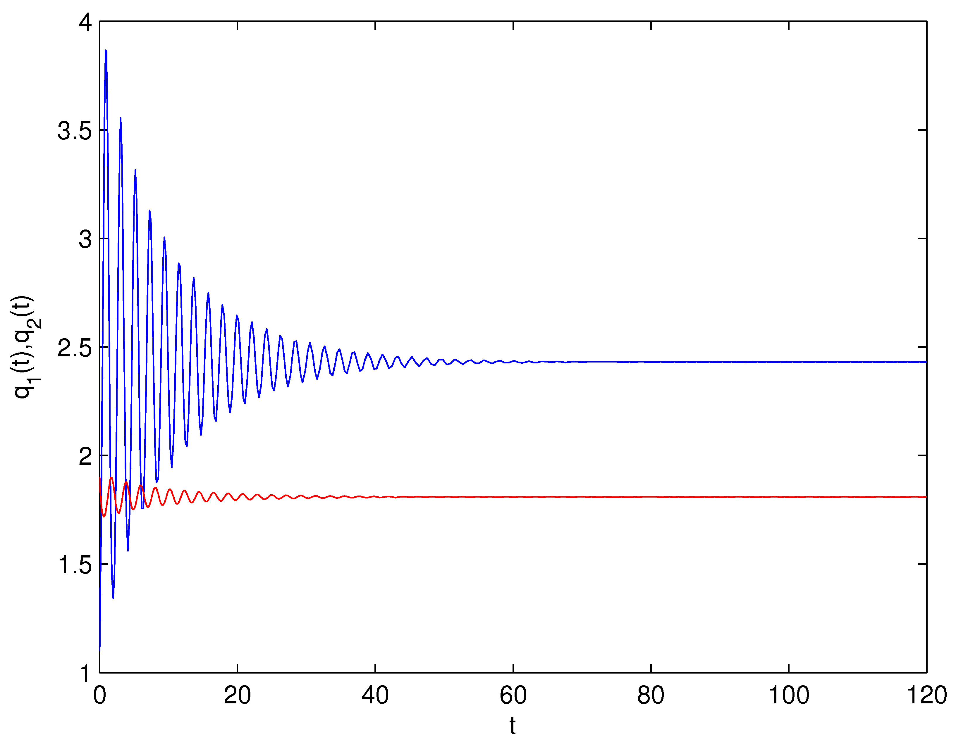
Figure 1. The time history plots of system (99) with ρ 1 = 0 , ρ 2 = 0.55 < ρ 20 0.59 . The locally asymptotically stable level of the positive equilibrium point Q 4 ( 2.4309 , 1.8090 ) of system (99). The blue line represents q 1 ( t ) and the red line represents q 2 ( t ) .
Fractalfract 07 00352 g001
Figure 2. The phase plot of system (99) with ρ 1 = 0 , ρ 2 = 0.55 < ρ 20 0.59 . The locally asymptotically stable level of the positive equilibrium point Q 4 ( 2.4309 , 1.8090 ) of system (99).
Fractalfract 07 00352 g002
Figure 3. The time history plots of system (99) with ρ 1 = 0 , ρ 2 = 0.7 > ρ 20 0.59 . The Hopf bifurcation phenomenon near the positive equilibrium point Q 4 ( 2.4309 , 1.8090 ) of system (99). The blue line represents q 1 ( t ) and the red line represents q 2 ( t ) .
Fractalfract 07 00352 g003
Figure 4. The phase plot of system (99) with ρ 1 = 0 , ρ 2 = 0.7 > ρ 20 0.59 . The Hopf bifurcation phenomenon near the positive equilibrium point Q 4 ( 2.4309 , 1.8090 ) of system (99).
Fractalfract 07 00352 g004
Figure 5. Bifurcation plot of system (99) with ρ 1 = 0 : the relation of t and q 1 . The bifurcation value ρ 20 0.59 .
Fractalfract 07 00352 g005
Figure 6. Bifurcation plot of system (99) with ρ 1 = 0 : the relation of t and q 2 . The bifurcation value ρ 20 0.59 .
Fractalfract 07 00352 g006
Figure 7. The time history plots of system (99) with ρ 2 = 0 , ρ 1 = 0.44 < ρ 10 0.48 . The locally asymptotically stable level of the positive equilibrium point Q 4 ( 2.4309 , 1.8090 ) of system (99). The blue line represents q 1 ( t ) and the red line represents q 2 ( t ) .
Fractalfract 07 00352 g007
Figure 8. The phase plot of system (99) with ρ 2 = 0 , ρ 1 = 0.44 < ρ 10 0.48 . The locally asymptotically stable level of the positive equilibrium point Q 4 ( 2.4309 , 1.8090 ) of system (99).
Fractalfract 07 00352 g008
Figure 9. The time history plots of system (99) with ρ 2 = 0 , ρ 1 = 0.44 > ρ 10 0.48 . The Hopf bifurcation phenomenon near the positive equilibrium point Q 4 ( 2.4309 , 1.8090 ) of system (99). The blue line represents q 1 ( t ) and the red line represents q 2 ( t ) .
Fractalfract 07 00352 g009
Figure 10. The phase plot of system (99) with ρ 2 = 0 , ρ 1 = 0.56 > ρ 10 0.48 . The Hopf bifurcation phenomenon near the positive equilibrium point Q 4 ( 2.4309 , 1.8090 ) of system (99).
Fractalfract 07 00352 g010
Figure 11. Bifurcation plot of system (99) with ρ 2 = 0 : the relation of t and q 1 . The bifurcation value ρ 10 0.48 .
Fractalfract 07 00352 g011
Figure 12. Bifurcation plot of system (99) with ρ 2 = 0 : the relation of t and q 2 . The bifurcation value ρ 10 0.48 .
Fractalfract 07 00352 g012
Figure 13. The time history plots of system (99) with ρ 2 = 0.5 , ρ 1 = 0.55 < ρ 1 0.61 . The locally asymptotically stable level of the positive equilibrium point Q 4 ( 2.4309 , 1.8090 ) of system (99). The blue line represents q 1 ( t ) and the red line represents q 2 ( t ) .
Fractalfract 07 00352 g013
Figure 14. The phase plot of system (99) with ρ 2 = 0.5 , ρ 1 = 0.67 < ρ 1 0.61 . The locally asymptotically stable level of the positive equilibrium point Q 4 ( 2.4309 , 1.8090 ) of system (99).
Fractalfract 07 00352 g014
Figure 15. The time history plots of system (99) with ρ 2 = 0.5 , ρ 1 = 0.67 > ρ 1 0.61 . The Hopf bifurcation phenomenon near the positive equilibrium point Q 4 ( 2.4309 , 1.8090 ) of system (99).
Fractalfract 07 00352 g015
Figure 16. The phase plot of system (99) with ρ 2 = 0.5 , ρ 1 = 0.67 > ρ 1 0.61 . The Hopf bifurcation phenomenon near the positive equilibrium point Q 4 ( 2.4309 , 1.8090 ) of system (99).
Fractalfract 07 00352 g016
Figure 17. Bifurcation plot of system (99) with ρ 2 = 0.5 : the relation of t and q 1 . The bifurcation value is ρ 1 0.59 .
Fractalfract 07 00352 g017
Figure 18. Bifurcation plot of system (99) with ρ 2 = 0.5 : the relation of t and q 2 . The bifurcation value is ρ 1 0.59 .
Fractalfract 07 00352 g018
Figure 19. The time history plots of system (99) with ρ 1 = 0.4 , ρ 2 = 0.45 < ρ 2 0.50 . The locally asymptotically stable level of the positive equilibrium point Q 4 ( 2.4309 , 1.8090 ) of system (99). The blue line represents q 1 ( t ) and the red line represents q 2 ( t ) .
Fractalfract 07 00352 g019
Figure 20. The phase plot of system (99) with ρ 1 = 0.4 , ρ 2 = 0.45 < ρ 2 0.50 . The locally asymptotically stable level of the positive equilibrium point Q 4 ( 2.4309 , 1.8090 ) of system (99).
Fractalfract 07 00352 g020
Figure 21. The time history plots of system (99) with ρ 1 = 0.4 , ρ 2 = 0.62 > ρ 2 0.50 . The Hopf bifurcation phenomenon near the positive equilibrium point Q 4 ( 2.4309 , 1.8090 ) of system (99).
Fractalfract 07 00352 g021
Figure 22. The phase plot of system (99) with ρ 1 = 0.4 , ρ 2 = 0.62 > ρ 2 0.50 . The Hopf bifurcation phenomenon near the positive equilibrium point Q 4 ( 2.4309 , 1.8090 ) of system (99).
Fractalfract 07 00352 g022
Figure 23. Bifurcation plot of system (99) with ρ 1 = 0.4 : the relation of t and q 2 . The bifurcation value ρ 2 0.50 .
Fractalfract 07 00352 g023
Figure 24. Bifurcation plot of system (99) with ρ 1 = 0.4 : the relation of t and q 2 . The bifurcation value ρ 2 0.50 .
Fractalfract 07 00352 g024
Figure 25. The time history plots of system (99) with ρ = 0.42 < ρ 0 0.49 . The locally asymptotically stable level of the positive equilibrium point Q 4 ( 2.4309 , 1.8090 ) of system (99). The blue line represents q 1 ( t ) and the red line represents q 2 ( t ) .
Fractalfract 07 00352 g025
Figure 26. The phase plot of system (99) with ρ = 0.42 < ρ 0 0.49 . The locally asymptotically stable level of the positive equilibrium point Q 4 ( 2.4309 , 1.8090 ) of system (99).
Fractalfract 07 00352 g026
Figure 27. The time history plots of system (99) with ρ = 0.53 > ρ 0 0.49 . The Hopf bifurcation phenomenon near the positive equilibrium point Q 4 ( 2.4309 , 1.8090 ) of system (99).
Fractalfract 07 00352 g027
Figure 28. The phase plot of system (99) with ρ = 0.53 > ρ 0 0.49 . The Hopf bifurcation phenomenon near the positive equilibrium point Q 4 ( 2.4309 , 1.8090 ) of system (99).
Fractalfract 07 00352 g028
Figure 29. Bifurcation plot of system (99) with ρ 1 = ρ 2 : the relation of t and q 1 . The bifurcation value ρ 0 0.49 .
Fractalfract 07 00352 g029
Figure 30. Bifurcation plot of system (99) with ρ 1 = ρ 2 : the relation of t and q 2 . The bifurcation value ρ 0 0.49 .
Fractalfract 07 00352 g030
Disclaimer/Publisher’s Note: The statements, opinions and data contained in all publications are solely those of the individual author(s) and contributor(s) and not of MDPI and/or the editor(s). MDPI and/or the editor(s) disclaim responsibility for any injury to people or property resulting from any ideas, methods, instructions or products referred to in the content.