Order of Convergence and Dynamics of Newton–Gauss-Type Methods

Abstract

On the basis of the new iterative technique designed by Zhongli Liu in 2016 with convergence orders of three and five, an extension to order six can be found in this paper. The study of high-convergence-order iterative methods under weak conditions is of extreme importance, because higher order means that fewer iterations are carried out to achieve a predetermined error tolerance. In order to enhance the practicality of these methods by Zhongli Liu, the convergence analysis is carried out without the application of Taylor expansion and requires the operator to be only two times differentiable, unlike the earlier studies. A semilocal convergence analysis is provided. Furthermore, numerical experiments verifying the convergence criteria, comparative studies and the dynamics are discussed for better interpretation.

1. Introduction

Driven by the needs of applications in applied mathematics, Refs. [1,2,3,4,5,6] finding a solution $x^{*}$ of the equation

$$\mathcal{L}\left(x\right)=0,$$

(1)

is considered significant, where $\mathcal{L}:\mathsf{\Omega }\in T\to T_1$ is a nonlinear Fréchet differentiable operator. Here and below, T and $T_1$ are Banach spaces and $\mathsf{\Omega }$ is an open convex set in $T.$ Due to the complexity in finding closed form solutions to (1), it is often advised to adopt iterative methods to find $x^{*}$. Newton’s method has been modified in numerous ways in the studies found in [7,8,9,10,11,12,13,14]. This paper is based on the Newton–Gauss iterative method studied by Zhongli Liu et al. in [15]. Precisely, in [15], Zhongli Liu et al. constructed the following method (see (2) below) by employing the two-point Gauss quadrature formula, given for each $n=0,1,2,\dots$ as

$$\begin{array}{ccc}\hfill y_n& =& x_n-{\mathcal{L}}^{\prime }{\left(x_n\right)}^{-1}\mathcal{L}\left(x_n\right)\hfill \\ \hfill x_{n+1}& =& x_n-2A_n^{-1}\mathcal{L}\left(x_n\right),\hfill \end{array}$$

(2)

where $A_n={\mathcal{L}}^{\prime }(u_n-v_n)+{\mathcal{L}}^{\prime }(u_n+v_n)$, $u_n=\frac{x_n+y_n}{2},v_n=\frac{y_n-x_n}{2\sqrt{3}}.$

This was further extended to a method of order five given by

$$\begin{array}{ccc}\hfill y_n& =& x_n-{\mathcal{L}}^{\prime }{\left(x_n\right)}^{-1}\mathcal{L}\left(x_n\right)\hfill \\ \hfill z_n& =& x_n-2A_n^{-1}\mathcal{L}\left(x_n\right),\hfill \\ \hfill x_{n+1}& =& z_n-{\mathcal{L}}^{\prime }{\left(y_n\right)}^{-1}\mathcal{L}\left(z_n\right).\hfill \end{array}$$

(3)

Recall [1] that a sequence $\left\{x_n\right\}$ converges to $x^{*}$ with convergence order $p>0,$ if for ${ϵ}_n^x=\parallel x_n-x^{*}\parallel ,$

$${ϵ}_{n+1}^x\le c{\left({ϵ}_n^x\right)}^p,$$

where c is called the rate of convergence.

The current level of research is established in [7,8,9,10,11,12,13,14,15]. In these references, the convergence order was established using higher order derivatives. Thus, these results cannot be applied to solve equations involving operators that are not at least five (if the order of the method is four) times differentiable. This limits their applicability, and other problems also exist:

(a)

No computable error bounds are provided;

(b)

There is no information on the uniqueness domain of the solution;

(c)

The local convergence analysis is provided only when $T=T_1={\mathbb{R}}^m$;

(d)

The more interesting (than the local) semilocal convergence analysis is not provided.

We address all of these concerns in the more general setting of a Banach space using generalized conditions and majorizing sequences. Moreover, our extended method (see (4)) is of order six, not five.

The study on the order of convergence of (2) and (3) in [15] involves Taylor expansion. The major concern in [15] is the necessity of assumptions on the derivatives of $\mathcal{L}$ up to order five, reducing the utility of the above methods. As an example, consider $f:[-2,2]⟶\mathbb{R}$ given by

$$\begin{array}{c}\hfill f\left(t\right)=\left\{\begin{array}{cc}\frac{1}{20}(t^{4}log{t}^2+t^6-t^5)\hfill & ift\in [-2,2]-\left\{0\right\}\hfill \\ 0\hfill & ift=0.\hfill \end{array}\right.\end{array}$$

It follows that

$$\begin{array}{ccc}\hfill f^{\prime }\left(t\right)& =& \frac{1}{20}(2t^3+4t^{3}log{t}^2+6t^5-5t^4)\hfill \\ \hfill f^{″}\left(t\right)& =& \frac{1}{20}(14t^2+12t^{2}log{t}^2+30t^4-20t^3)\hfill \\ \hfill f^{″\prime }\left(t\right)& =& \frac{1}{20}(52t+24tlog{t}^2+120t^3-60t^2)\hfill \\ \hfill f^{IV}\left(t\right)& =& \frac{1}{20}(24log{t}^2+360t^2-120t+100).\hfill \end{array}$$

Observe that $f^{IV}\left(t\right)$ is not bounded.

Our study is solely based on obtaining the required order of convergence of the above methods without using Taylor expansion and assumptions only on ${\mathcal{L}}^{\prime }$ and ${\mathcal{L}}^{″}.$ This enhances the applicability of the considered iterative method to a wider range of practical problems. Our approach can be used to study other similar methods [5,6,16,17,18].

Furthermore, we have extended this to a method of order six with the ideas in [3,4] defined for $n=0,1,2,\dots$ given by

$$\begin{array}{ccc}\hfill y_n& =& x_n-{\mathcal{L}}^{\prime }{\left(x_n\right)}^{-1}\mathcal{L}\left(x_n\right)\hfill \\ \hfill z_n& =& x_n-2A_n^{-1}\mathcal{L}\left(x_n\right),\hfill \\ \hfill x_{n+1}& =& z_n-{\mathcal{L}}^{\prime }{\left(z_n\right)}^{-1}\mathcal{L}\left(z_n\right).\hfill \end{array}$$

(4)

The outline of the article is as follows. We discuss the convergence of the methods (2), (3) and (4) in Section 2, Section 3 and Section 4 respectively. Semilocal convergence of the methods is developed in Section 5. Section 6 deals with examples. Section 7 is dedicated to the dynamics and the basins of attraction of the methods (2), (3) and (4). Section 8 gives the conclusion.

2. Convergence Analysis of (2)

Hereafter, $B(x^{*},\tau )=\{x\in T:\parallel x-x^{*}\parallel <\tau \}$ and $\overline{B}(x^{*},\tau )=\{x\in T:\parallel x-x^{*}\parallel \le \tau \}$ for some $\tau >0.$

The following assumptions are made in our study:

(A1)

a simple solution $x^{*}$ of (1) exists and ${\mathcal{L}}^{\prime }{\left(x^{*}\right)}^{-1}\in L(T_1,T)$;

(A2)

$\parallel {\mathcal{L}}^{\prime }{\left(x^{*}\right)}^{-1}({\mathcal{L}}^{\prime }\left(w_1\right)-{\mathcal{L}}^{\prime }\left(w_2\right))\parallel \le L\parallel w_1-w_2\parallel \forall w_1,w_2\in \mathsf{\Omega };$

(A3)

$\parallel {\mathcal{L}}^{\prime }{\left(x^{*}\right)}^{-1}({\mathcal{L}}^{″}\left(w_1\right)-{\mathcal{L}}^{″}\left(w_2\right))\parallel \le L_2\parallel w_1-w_2\parallel \forall w_1,w_2\in \mathsf{\Omega }$;

(A4)

$\parallel {\mathcal{L}}^{\prime }{\left(x^{*}\right)}^{-1}{\mathcal{L}}^{″}\left(w_2\right)\parallel \le L_1\forall w_2\in \mathsf{\Omega }$;

(A5)

$\parallel {\mathcal{L}}^{\prime }{\left(w_1\right)}^{-1}({\mathcal{L}}^{\prime }\left(w_1\right)-{\mathcal{L}}^{\prime }\left(w_2\right))\parallel \le L_3\parallel w_1-w_2\parallel \forall w_1,w_2\in \mathsf{\Omega }.$

(A6)

$B(x^{*},\left(\frac{1+\sqrt{3}}{\sqrt{3}}\right)r)\subset \mathsf{\Omega },$ for parameter $r>0$ to be specified in what follows and $L>0,L_1>0,L_2>0$ and $L_3>0$ are scalars.

We define the functions $\varphi ,{\varphi }_1,h_1:[0,\frac{1}{L})⟶\mathbb{R}$ by

$$\varphi \left(t\right)=\frac{L}{2(1-Lt)},$$

$${\varphi }_1\left(t\right)=\frac{L}{2}\left(1+\frac{L}{2(1-Lt)}t\right)$$

and let $h_1\left(t\right)={\varphi }_1\left(t\right)t-1.$ Observe that $h_1$ is a continuous nondecreasing function. Furthermore, $h_1\left(0\right)=-1<0$ and ${lim}_{t⟶{\frac{1}{L}}^{-}}{h}_1\left(t\right)=+\infty .$ Therefore, there exists a smallest zero $r_1\in (0,\frac{1}{L})$ for $h_1\left(t\right)=0.$

Let the functions ${\varphi }_2,h_2:[0,\frac{1}{L})⟶\mathbb{R}$ be defined by

$${\varphi }_2\left(t\right)=\frac{1}{1-{\varphi }_1\left(t\right)t}\left[\frac{(1+\sqrt{3})L_1\varphi \left(t\right)}{2\sqrt{3}}+\frac{L_2(1+\varphi \left(t\right)t)}{24}\right]$$

and $h_2\left(t\right)={\varphi }_2\left(t\right)t^2-1.$ Observe that $h_2$ is a nondecreasing and continuous function, $h_2\left(0\right)=-1<0$ and ${lim}_{t⟶r_1^{-}}{h}_2\left(t\right)=+\infty .$ Therefore, $h_2$ has a smallest zero $\rho \in (0,r_1).$

Let

$$r=min\{\frac{2}{3L},\rho \}.$$

(5)

Then, $0\le \varphi \left(t\right)t<1,$$0\le {\varphi }_1\left(t\right)t<1$ and $0\le {\varphi }_2\left(t\right)t^2<1,$∀$t\in [0,r).$

For convenience, we use the notation ${ϵ}_n^x=\parallel x_n-x^{*}\parallel ,{ϵ}_n^y=\parallel y_n-x^{*}\parallel ,$${ϵ}_n^z=\parallel z_n-x^{*}\parallel$ and $B^{*}=B(x^{*},r)-\left\{x^{*}\right\}.$

Theorem 1.

Assume (A1)–(A6) hold, and let r be as in (5). Then, the sequence $\left\{x_n\right\}$ given by the formula (2), for $x_0\in B^{*}$ exists, $x_n\in \overline{B}(x^{*},r)$$\forall n=0,1,2,\dots$ and ${lim}_{n⟶\infty }{x}_n=x^{*}.$ Furthermore,

$${ϵ}_n^y\le \varphi \left(r\right){\left({ϵ}_n^x\right)}^2$$

(6)

and

$${ϵ}_{n+1}^x\le {\varphi }_2\left(r\right){\left({ϵ}_n^x\right)}^3.$$

(7)

Proof. 

This is proved utilizing induction. Let $x\in B(x^{*},r).$ Using (A2) gives

$$\parallel {\mathcal{L}}^{\prime }{\left(x^{*}\right)}^{-1}({\mathcal{L}}^{\prime }\left(x\right)-{\mathcal{L}}^{\prime }\left(x^{*}\right))\parallel \le L\parallel x-x^{*}\parallel \le Lr<1.$$

By the Banach result on invertible operators [1,2], it follows that

$$\parallel {\mathcal{L}}^{\prime }{\left(x\right)}^{-1}{\mathcal{L}}^{\prime }\left(x^{*}\right)\parallel \le \frac{1}{1-L\parallel x-x^{*}\parallel }.$$

(8)

The Mean Value Theorem (MVT) leads to

$$\begin{array}{c}\hfill \mathcal{L}\left(\xi \right)=\mathcal{L}\left(\xi \right)-\mathcal{L}\left(x^{*}\right)={\int }_0^1{\mathcal{L}}^{\prime }(x^{*}+t(\xi -x^{*}))dt(\xi -x^{*}),\end{array}$$

(9)

for any $\xi \in T.$ Next, because $y_0=x_0-{\mathcal{L}}^{\prime }{\left(x_0\right)}^{-1}\mathcal{L}\left(x_0\right),$ by (9) (with $\xi =x_0$), we have

$$\begin{array}{ccc}\hfill {ϵ}_0^y& =& \parallel x_0-x^{*}-{\mathcal{L}}^{\prime }{\left(x_0\right)}^{-1}\mathcal{L}\left(x_0\right)\parallel \hfill \\ & =& ∥(x_0-x^{*})-{\mathcal{L}}^{\prime }{\left(x_0\right)}^{-1}{\int }_0^1{\mathcal{L}}^{\prime }(x^{*}+t(x_0-x*))dt(x_0-x^{*})∥\hfill \\ & =& ∥\left({\int }_0^1{\mathcal{L}}^{\prime }{\left(x_0\right)}^{-1}({\mathcal{L}}^{\prime }\left(x_0\right)-{\mathcal{L}}^{\prime }(x^{*}+t(x_0-x^{*})))dt\right)(x_0-x^{*})∥\hfill \\ & \le & {\int }_0^1\parallel {\mathcal{L}}^{\prime }{\left(x_0\right)}^{-1}({\mathcal{L}}^{\prime }\left(x_0\right)-{\mathcal{L}}^{\prime }(x^{*}+t(x_0-x^{*})))\parallel dt{ϵ}_0^x\hfill \\ & =& {\int }_0^1\parallel {\mathcal{L}}^{\prime }{\left(x_0\right)}^{-1}{\mathcal{L}}^{\prime }\left(x^{*}\right){\mathcal{L}}^{\prime }{\left(x^{*}\right)}^{-1}({\mathcal{L}}^{\prime }\left(x_0\right)-{\mathcal{L}}^{\prime }(x^{*}+t(x_0-x^{*})))dt\parallel {ϵ}_0^x.\hfill \end{array}$$

Thus, by our assumptions,

$$\begin{array}{ccc}\hfill {ϵ}_0^y& \le & \frac{L}{2(1-L{ϵ}_0^x)}{\left({ϵ}_0^x\right)}^2\hfill \\ & \le & \varphi \left({ϵ}_0^x\right){\left({ϵ}_0^x\right)}^2<{ϵ}_0^x<r.\hfill \end{array}$$

(10)

So, the iterate $y_0\in B(x^{*},r)$ and the result holds for $n=0.$ In addition, $A_0^{-1}$ is well defined. In fact,

$$\begin{array}{ccc}\hfill \parallel {\left(2{\mathcal{L}}^{\prime }\left(x^{*}\right)\right)}^{-1}(A_0-2{\mathcal{L}}^{\prime }\left(x^{*}\right))\parallel & =& \parallel {\left(2{\mathcal{L}}^{\prime }\left(x^{*}\right)\right)}^{-1}({\mathcal{L}}^{\prime }(u_0-v_0)+{\mathcal{L}}^{\prime }(u_0+v_0)-2{\mathcal{L}}^{\prime }\left(x^{*}\right))\parallel \hfill \\ \hfill & =& \frac{1}{2}\parallel {\mathcal{L}}^{\prime }{\left(x^{*}\right)}^{-1}({\mathcal{L}}^{\prime }\left(\frac{(1+\sqrt{3})x_0+(\sqrt{3}-1)y_0}{2\sqrt{3}}\right)-{\mathcal{L}}^{\prime }\left(x^{*}\right))\hfill \\ \hfill & & +{\mathcal{L}}^{\prime }{\left(x^{*}\right)}^{-1}({\mathcal{L}}^{\prime }\left(\frac{(\sqrt{3}-1)x_0+(\sqrt{3}+1)y_0}{2\sqrt{3}}\right)-{\mathcal{L}}^{\prime }\left(x^{*}\right))\parallel \hfill \\ \hfill & \le & \frac{L}{2}\left[\parallel \frac{(1+\sqrt{3})x_0+(\sqrt{3}-1)y_0}{2\sqrt{3}}-x^{*}\parallel \right.\hfill \\ \hfill & & +\left.\parallel \frac{(\sqrt{3}-1)x_0+(\sqrt{3}+1)y_0}{2\sqrt{3}}-x^{*}\parallel \right]\hfill \\ \hfill & \le & \frac{L}{2}[{ϵ}_0^x+{ϵ}_0^y]\hfill \\ \hfill & \le & \frac{L}{2}[1+\frac{L}{2(1-Lr)}{ϵ}_0^x]{ϵ}_0^x\hfill \\ \hfill & \le & {\varphi }_1\left(r\right){ϵ}_0^x\le 1,\hfill \end{array}$$

(11)

where we also used

$$\parallel u_0+v_0-x^{*}\parallel =∥\frac{\sqrt{3}(x_0-x^{*})+\sqrt{3}(y_0-x^{*})+(y_0-x^{*})+(x^{*}-x_0)}{2\sqrt{3}}∥\le \left(\frac{1+\sqrt{3}}{\sqrt{3}}\right)r$$

and

$$\parallel u_0-v_0-x^{*}\parallel =∥\frac{\sqrt{3}(x_0-x^{*})+\sqrt{3}(y_0-x^{*})+(x_0-x^{*})+(x^{*}-y_0)}{2\sqrt{3}}∥\le \left(\frac{1+\sqrt{3}}{\sqrt{3}}\right)r.$$

That is $u_0+v_0,u_0-v_0\in B(x^{*},\left(\frac{1+\sqrt{3}}{\sqrt{3}}\right)r).$ Therefore, by Banach lemma on invertible operators [1] $A_0^{-1}$ exists and

$$\begin{array}{ccc}\hfill \parallel A_0^{-1}{\mathcal{L}}^{\prime }\left(x^{*}\right)\parallel & \le & \frac{1}{2(1-{\varphi }_1\left({ϵ}_0^x\right){ϵ}_0^x)}\hfill \end{array}$$

(12)

From (2) and (9), we obtain

$$\begin{array}{ccc}\hfill x_1-x^{*}& =& x_0-x^{*}-2A_0^{-1}\mathcal{L}\left(x_0\right)\hfill \\ & =& A_0^{-1}(A_0-2{\int }_0^1{\mathcal{L}}^{\prime }(x^{*}+t(x_0-x^{*}))dt)(x_0-x^{*})\hfill \\ & =& A_0^{-1}({\mathcal{L}}^{\prime }(u_0-v_0)+{\mathcal{L}}^{\prime }(u_0+v_0)-2{\int }_0^1{\mathcal{L}}^{\prime }(x^{*}+t(x_0-x^{*}))dt)(x_0-x^{*})\hfill \\ & =& A_0^{-1}[{\mathcal{L}}^{\prime }\left(\frac{x_0(1+\sqrt{3})+y_0(\sqrt{3}-1)}{2\sqrt{3}}\right)+{\mathcal{L}}^{\prime }\left(\frac{x_0(\sqrt{3}-1)+y_0(\sqrt{3}+1)}{2\sqrt{3}}\right)\hfill \\ & & -2{\int }_0^1{\mathcal{L}}^{\prime }(x^{*}+t(x_0-x^{*}))dt](x_0-x^{*})\hfill \\ & =& A_0^{-1}\left[{\int }_0^1{\mathcal{L}}^{\prime }\left(\frac{x_0(1+\sqrt{3})+y_0(\sqrt{3}-1)}{2\sqrt{3}}\right)-{\mathcal{L}}^{\prime }(x^{*}+t(x_0-x^{*}))dt\right](x_0-x^{*})\hfill \\ & & +A_0^{-1}\left[{\int }_0^1{\mathcal{L}}^{\prime }\left(\frac{x_0(\sqrt{3}-1)+y_0(\sqrt{3}+1)}{2\sqrt{3}}\right)-{\mathcal{L}}^{\prime }(x^{*}+t(x_0-x^{*}))dt\right]\hfill \\ & & \times (x_0-x^{*}).\hfill \end{array}$$

(13)

Let

$$\begin{array}{ccc}\hfill G_0(\theta ,t)& =& {\mathcal{L}}^{″}\left(x^{*}+t(x_0-x^{*})+\theta \left(\frac{x_0(1+\sqrt{3})+y_0(\sqrt{3}-1)}{2\sqrt{3}}-x^{*}-t(x_0-x^{*})\right)\right)\hfill \\ \hfill H_0(\theta ,t)& =& {\mathcal{L}}^{″}\left(x^{*}+t(x_0-x^{*})+\theta \left(\frac{x_0(\sqrt{3}-1)+y_0(\sqrt{3}+1)}{2\sqrt{3}}-x^{*}-t(x_0-x^{*})\right)\right)\hfill \end{array}$$

By (MVT) for second derivatives, (12) gives

$$\begin{array}{ccc}\hfill x_1-x^{*}& =& A_0^{-1}[{\int }_0^1{\int }_0^1{G}_0(\theta ,t)d\theta \left(\frac{x_0(1+\sqrt{3})+y_0(\sqrt{3}-1)}{2\sqrt{3}}-x^{*}-t(x_0-x^{*})\right)dt\hfill \\ & & +{\int }_0^1{\int }_0^1{H}_0(\theta ,t)d\theta \left(\frac{x_0(\sqrt{3}-1)+y_0(\sqrt{3}+1)}{2\sqrt{3}}-x^{*}-t(x_0-x^{*})\right)dt](x_0-x^{*})\hfill \\ & =& \frac{A_0^{-1}}{2\sqrt{3}}\left[{\int }_0^1{\int }_0^1{G}_0(\theta ,t)d\theta \right(x_0-x^{*}-(y_0-x^{*})+\sqrt{3}(x_0-x^{*})+\sqrt{3}(y_0-x^{*})\hfill \\ & & -2\sqrt{3}t(x_0-x^{*}))dt+{\int }_0^1{\int }_0^1{H}_0(\theta ,t)d\theta (y_0-x^{*}+x^{*}-x_0+\sqrt{3}(x_0-x^{*})\hfill \\ & & +\sqrt{3}(y_0-x^{*})-2\sqrt{3}t(x_0-x^{*})\left)dt\right](x_0-x^{*})\hfill \\ & =& \frac{A_0^{-1}}{2}\left[{\int }_0^1{\int }_0^1{G}_0(\theta ,t)d\theta (x_0-x^{*})(1-2t)dt\right](x_0-x^{*})\hfill \\ & & -\frac{(1+\sqrt{3})A_0^{-1}}{2\sqrt{3}}\left[{\int }_0^1{\int }_0^1{G}_0(\theta ,t)d\theta (y_0-x^{*})dt\right](x_0-x^{*})\hfill \\ & & +\frac{A_0^{-1}}{2}\left[{\int }_0^1{\int }_0^1{H}_0(\theta ,t)d\theta \left((x_0-x^{*})(1-2t)dt\right)\right](x_0-x^{*})\hfill \\ & & +\frac{(1+\sqrt{3})A_0^{-1}}{2\sqrt{3}}\left[{\int }_0^1{\int }_0^1{H}_0(\theta ,t)d\theta (y_0-x^{*})dt\right](x_0-x^{*})\hfill \\ & & +\frac{A_0^{-1}}{2\sqrt{3}}\left[{\int }_0^1{\int }_0^1(G_0(\theta ,t)-H_0(\theta ,t))d\theta dt\right]{(x_0-x^{*})}^2\hfill \\ & =:& {\mathbb{M}}_1+{\mathbb{M}}_2+{\mathbb{M}}_3+{\mathbb{M}}_4+{\mathbb{M}}_5,\hfill \end{array}$$

(14)

where

$$\begin{array}{ccc}\hfill {\mathbb{M}}_1& =& \frac{A_0^{-1}}{2}\left[{\int }_0^1{\int }_0^1{G}_0(\theta ,t)d\theta (1-2t)dt\right]{(x_0-x^{*})}^2\hfill \\ \hfill {\mathbb{M}}_2& =& -\frac{(1+\sqrt{3})A_0^{-1}}{2\sqrt{3}}\left[{\int }_0^1{\int }_0^1{G}_0(\theta ,t)d\theta (y_0-x^{*})dt\right](x_0-x^{*})\hfill \\ \hfill {\mathbb{M}}_3& =& \frac{A_0^{-1}}{2}\left[{\int }_0^1{\int }_0^1{H}_0(\theta ,t)d\theta \left((x_0-x^{*})(1-2t)dt\right)\right](x_0-x^{*})\hfill \\ \hfill {\mathbb{M}}_4& =& \frac{(1+\sqrt{3})A_0^{-1}}{2\sqrt{3}}\left[{\int }_0^1{\int }_0^1{H}_0(\theta ,t)d\theta (y_0-x^{*})dt\right](x_0-x^{*})\hfill \end{array}$$

and

$${\mathbb{M}}_5=\frac{A_0^{-1}}{2\sqrt{3}}\left[{\int }_0^1{\int }_0^1(G_0(\theta ,t)-H_0(\theta ,t))d\theta dt\right]{(x_0-x^{*})}^2.$$

Then, by (12) and assumption (A4),

$$\begin{array}{ccc}\hfill \parallel {\mathbb{M}}_1\parallel & =& ∥\frac{A_0^{-1}}{2}{\int }_0^1{\int }_0^1{G}_0(\theta ,t)d\theta (1-2t)dt{(x_0-x^{*})}^2∥\hfill \\ & \le & \parallel \frac{A_0^{-1}}{2}{\mathcal{L}}^{\prime }\left(x^{*}\right)\parallel ∥\parallel \underset{t}{max}{\int }_0^1{\mathcal{L}}^{\prime }{\left(x^{*}\right)}^{-1}{G}_0(\theta ,t)d\theta \parallel {\int }_0^1(1-2t){(x_0-x^{*})}^{2}dt∥\hfill \\ & =& 0.\hfill \end{array}$$

(15)

Similarly, one can observe

$$\begin{array}{ccc}\hfill \parallel {\mathbb{M}}_3\parallel & =& 0.\hfill \end{array}$$

(16)

By the assumptions(A1)–(A5) and (12), we get

$$\begin{array}{ccc}\hfill \parallel {\mathbb{M}}_2\parallel & =& ∥\frac{(1+\sqrt{3})A_0^{-1}}{2\sqrt{3}}{\mathcal{L}}^{\prime }\left(x^{*}\right){\int }_0^1{\int }_0^1{\mathcal{L}}^{\prime }{\left(x^{*}\right)}^{-1}{G}_0(\theta ,t)d\theta (y_0-x^{*})dt(x_0-x^{*})∥\hfill \\ & \le & \frac{1+\sqrt{3}}{2\sqrt{3}}\frac{L_1}{2(1-{\varphi }_1\left({ϵ}_0^x\right){ϵ}_0^x)}{ϵ}_0^y{ϵ}_0^x.\hfill \end{array}$$

(17)

Similarly,

$$\parallel {\mathbb{M}}_4\parallel \le \frac{1+\sqrt{3}}{2\sqrt{3}}\frac{L_1}{2(1-{\varphi }_1\left({ϵ}_0^x\right){ϵ}_0^x)}{ϵ}_0^y{ϵ}_0^x$$

(18)

Note that

$$\begin{array}{ccc}\hfill G_0(\theta ,t)-H_0(\theta ,t)& =& {\mathcal{L}}^{″}\left(X_1\right)-{\mathcal{L}}^{″}\left(X_2\right),\hfill \end{array}$$

where

$$\begin{array}{ccc}\hfill X_1& =& x^{*}+t(x_0-x^{*})+\theta \left(\frac{x_0(1+\sqrt{3})+y_0(\sqrt{3}-1)}{2\sqrt{3}}-x^{*}-t(x_0-x^{*})\right),\hfill \\ \hfill X_2& =& x^{*}+t(x_0-x^{*})+\theta \left(\frac{x_0(\sqrt{3}-1)+y_0(\sqrt{3}+1)}{2\sqrt{3}}-x^{*}-t(x_0-x^{*})\right).\hfill \end{array}$$

Then

$$\begin{array}{ccc}\hfill X_1-X_2& =& \frac{\theta }{\sqrt{3}}(x_0-x^{*}-(y_0-x^{*}))\hfill \end{array}$$

So, by (12) and assumption (A3),

$$\begin{array}{ccc}\hfill \parallel {\mathbb{M}}_5\parallel & =& ∥\frac{A_0^{-1}}{2\sqrt{3}}{\mathcal{L}}^{\prime }\left(x^{*}\right){\int }_0^1{\int }_0^1{\mathcal{L}}^{\prime }{\left(x^{*}\right)}^{-1}(G_0(\theta ,t)-H_0(\theta ,t))d\theta dt{(x_0-x^{*})}^2∥\hfill \\ & \le & \frac{L_2}{4\sqrt{3}(1-{\varphi }_1\left({ϵ}_0^x\right){ϵ}_0^x)}{\int }_0^1{\int }_0^1\parallel X_1-X_2\parallel d\theta dt{\left({ϵ}_0^x\right)}^2\hfill \\ & \le & \frac{L_2}{4\sqrt{3}(1-{\varphi }_1\left({ϵ}_0^x\right){ϵ}_0^x)}{\int }_0^1{\int }_0^1\frac{\theta }{\sqrt{3}}(x_0-x^{*}-(y_0-x^{*}))d\theta dt{\left({ϵ}_0^x\right)}^2\hfill \\ & \le & \frac{L_2}{24(1-{\varphi }_1\left({ϵ}_0^x\right){ϵ}_0^x)}[{ϵ}_0^x+{ϵ}_0^y]{\left({ϵ}_0^x\right)}^2\hfill \\ & \le & \frac{L_2}{24(1-{\varphi }_1\left({ϵ}_0^x\right){ϵ}_0^x)}[{ϵ}_0^x+\varphi \left({ϵ}_0^x\right){\left({ϵ}_0^x\right)}^2]{\left({ϵ}_0^x\right)}^2\hfill \\ & \le & \frac{L_2}{24(1-{\varphi }_1\left({ϵ}_0^x\right){ϵ}_0^x)}[1+\varphi \left({ϵ}_0^x\right){ϵ}_0^x]{\left({ϵ}_0^x\right)}^3.\hfill \end{array}$$

(19)

Combining (14)–(19) gives

$$\begin{array}{ccc}\hfill {ϵ}_1^x& \le & \parallel {\mathbb{M}}_1\parallel +\parallel {\mathbb{M}}_2\parallel +\parallel {\mathbb{M}}_3\parallel +\parallel {\mathbb{M}}_4\parallel +\parallel {\mathbb{M}}_5\parallel \hfill \\ & \le & \frac{1+\sqrt{3}}{2\sqrt{3}}\frac{L_1}{(1-{\varphi }_1\left({ϵ}_0^x\right){ϵ}_0^x)}\varphi \left({ϵ}_0^x\right){\left({ϵ}_0^x\right)}^3\hfill \\ & & +\frac{L_2}{24(1-{\varphi }_1\left({ϵ}_0^x\right){ϵ}_0^x)}[1+\varphi \left({ϵ}_0^x\right){ϵ}_0^x]{\left({ϵ}_0^x\right)}^3\hfill \\ & \le & \frac{1}{1-{\varphi }_1\left({ϵ}_0^x\right){ϵ}_0^x}\hfill \\ & & \times \left[\frac{1+\sqrt{3}}{2\sqrt{3}}{L}_1\varphi \left({ϵ}_0^x\right)+\frac{L_2}{24}(1+\varphi \left({ϵ}_0^x\right){ϵ}_0^x)\right]{\left({ϵ}_0^x\right)}^3\hfill \\ & \le & {\varphi }_2\left(r\right){\left({ϵ}_0^x\right)}^3.\hfill \end{array}$$

Therefore, because ${\varphi }_2\left(r\right)r^2<1,$ we have $\parallel x_1-x^{*}\parallel <r$, so the iterate $x_1\in B(x^{*},r)$.

The induction for (6) and (7) is completed, if one replaces $x_0,y_0,x_1$ in the above conclusions with $x_n,y_n,x_{n+1},$ respectively. □

3. Convergence Analysis of (3)

Let ${\varphi }_3,h_3:[0,r_1)⟶\mathbb{R}$ be given as

$${\varphi }_3\left(t\right)=L_3(\varphi \left(t\right)+\frac{1}{2}{\varphi }_2\left(t\right)t){\varphi }_2\left(t\right)$$

and $h_3\left(t\right)={\varphi }_3\left(t\right)t^4-1.$ Then, $h_3\left(0\right)=-1$ and ${lim}_{t⟶r_1^{-}}{h}_3\left(t\right)=+\infty .$ Therefore, $h_3$ has a smallest zero $r_2\in (0,r_1).$ Let

$$R=min\{r,r_2\}.$$

(20)

Then,

$$0\le {\varphi }_3\left(t\right)t^4<1\forall t\in [0,R).$$

Set $B_1^{*}=B(x^{*},R)-\left\{x^{*}\right\}.$ For Method (3), we have the following theorem:

Theorem 2.

Assume (A1)–(A6) hold, and let R be as in (20). Then, the sequence $\left\{x_n\right\}$ given by the formula (3), for $x_0\in B_1^{*}$ exists, $x_n\in \overline{B}(x^{*},R)$$\forall n=0,1,2,\dots$ and ${lim}_{n⟶\infty }{x}_n=x^{*}.$ Furthermore,

$$\begin{array}{ccc}\hfill {ϵ}_n^y& \le & \varphi \left(R\right){\left({ϵ}_n^x\right)}^2,\hfill \end{array}$$

(21)

$$\begin{array}{ccc}\hfill {ϵ}_n^z& \le & {\varphi }_2\left(R\right){\left({ϵ}_n^x\right)}^3\hfill \end{array}$$

(22)

and

$$\begin{array}{ccc}\hfill {ϵ}_{n+1}^x& \le & {\varphi }_3\left(R\right){\left({ϵ}_n^x\right)}^5.\hfill \end{array}$$

(23)

Proof. 

Note that (21) and (22) follow as in Theorem 1, by letting $r=R$ and $x_{n+1}=z_n$ in Theorem 1 and hence $z_n\in B(x^{*},R).$ Observe

$$\begin{array}{ccc}\hfill x_{n+1}-x^{*}& =& z_n-x^{*}-{\mathcal{L}}^{\prime }{\left(y_n\right)}^{-1}\mathcal{L}\left(z_n\right)\hfill \\ & =& {\mathcal{L}}^{\prime }{\left(y_n\right)}^{-1}{\int }_0^1[{\mathcal{L}}^{\prime }\left(y_n\right)-{\mathcal{L}}^{\prime }(x^{*}+t(z_n-x^{*}))]dt(z_n-x^{*})\hfill \\ & =& {\int }_0^1{\mathcal{L}}^{\prime }{\left(y_n\right)}^{-1}[{\mathcal{L}}^{\prime }\left(y_n\right)-{\mathcal{L}}^{\prime }(x^{*}+t(z_n-x^{*}))]dt(z_n-x^{*}).\hfill \end{array}$$

So, by (A5), we get

$$\begin{array}{ccc}\hfill {ϵ}_{n+1}^x& \le & L_3({ϵ}_n^y+\frac{1}{2}{ϵ}_n^z){ϵ}_n^z\hfill \\ & \le & L_3(\varphi \left({ϵ}_n^x\right){\left({ϵ}_n^x\right)}^2\hfill \\ & & +\frac{1}{2}{\varphi }_2\left({ϵ}_n^x\right){\left({ϵ}_n^x\right)}^3){\varphi }_2\left({ϵ}_n^x\right){\left({ϵ}_n^x\right)}^3\hfill \\ & \le & L_3(\varphi \left({ϵ}_n^x\right)\hfill \\ & & +\frac{1}{2}{\varphi }_2\left({ϵ}_n^x\right){ϵ}_n^x){\varphi }_2\left({ϵ}_n^x\right){\left({ϵ}_n^x\right)}^5\hfill \\ & \le & {\varphi }_3\left(R\right){\left({ϵ}_n^x\right)}^5.\hfill \end{array}$$

□

4. Convergence Analysis of (4)

Let ${\varphi }_4,h_4:[0,r_1)⟶\mathbb{R}$ be given by

$${\varphi }_4\left(t\right)=\frac{L_3}{2}{\left({\varphi }_2\left(t\right)\right)}^2$$

and $h_5\left(t\right)={\varphi }_4\left(t\right)t^5-1.$ Then, $h_4\left(0\right)=-1$ and ${lim}_{t⟶r_1^{-}}{h}_4\left(t\right)=\infty .$ Therefore, $h_4$ has a smallest zero $r_3\in (0,r_1).$

Let

$$R_1=min\{r,r_3\}.$$

(24)

Then,

$$0\le {\varphi }_4\left(t\right)t^5<1\forall t\in [0,R_1).$$

Set $B_2^{*}=B(x^{*},R_1)-\left\{x^{*}\right\}.$ Similarly, for Method (4), we develop:

Theorem 3.

Assume that (A1)–(A6) hold, and let $R_1$ be as in (24). Then, the sequence $\left\{x_n\right\}$ given by the formula (4), for $x_0\in B_2^{*}$ exists, $x_n\in \overline{B}(x^{*},R_1)$$\forall n=0,1,2,\dots$ and ${lim}_{n⟶\infty }{x}_n=x^{*}.$ Furthermore,

$${ϵ}_n^y\le \varphi \left(R_1\right){\left({ϵ}_n^x\right)}^2,$$

(25)

$${ϵ}_n^z\le {\varphi }_2\left(R_1\right){\left({ϵ}_n^x\right)}^3$$

(26)

and

$${ϵ}_{n+1}^x\le {\varphi }_4\left(R_1\right){\left({ϵ}_n^x\right)}^6.$$

(27)

Proof. 

Observe that (25) and (26) follow as in Theorem 2. Note that

$$\begin{array}{ccc}\hfill x_{n+1}-x^{*}& =& z_n-x^{*}-{\mathcal{L}}^{\prime }{\left(z_n\right)}^{-1}\mathcal{L}\left(z_n\right)\hfill \\ & =& {\mathcal{L}}^{\prime }{\left(z_n\right)}^{-1}{\int }_0^1[{\mathcal{L}}^{\prime }\left(z_n\right)-{\mathcal{L}}^{\prime }(x^{*}+t(z_n-x^{*}))]dt(z_n-x^{*})\hfill \\ & =& {\int }_0^1{\mathcal{L}}^{\prime }{\left(z_n\right)}^{-1}[{\mathcal{L}}^{\prime }\left(z_n\right)-{\mathcal{L}}^{\prime }(x^{*}+t(z_n-x^{*}))]dt(z_n-x^{*}).\hfill \end{array}$$

Hence, by (A5), we have

$$\begin{array}{ccc}\hfill {ϵ}_{n+1}^x& \le & \frac{L_3}{2}{\left({ϵ}_n^z\right)}^2\hfill \\ & \le & \frac{L_3}{2}{\left({\varphi }_2\left({ϵ}_n^x\right)\right)}^2{\left({ϵ}_n^x\right)}^6\hfill \\ & \le & {\varphi }_4\left(R_1\right){\left({ϵ}_n^x\right)}^6.\hfill \end{array}$$

□

Next, we provide a uniqueness result of the solution $x^{*}.$

Proposition 1.

Suppose:

(1) $\exists x^{*}\in B(x^{*},\rho )$ such that $\mathcal{L}\left(x^{*}\right)=0$ for some $\rho >0$ and $\exists K>0$ such that

$$\parallel {\mathcal{L}}^{\prime }{\left(x^{*}\right)}^{-1}({\mathcal{L}}^{\prime }\left(x^{*}\right)-{\mathcal{L}}^{\prime }\left(x\right))\parallel \le K\parallel x^{*}-x\parallel$$

(28)

for each $x\in B(x^{*},\rho ).$

(2) $\exists {\rho }_1\ge \rho$ such that

$${\rho }_1<\frac{2}{K}.$$

(29)

Let $S=\overline{B}(x^{*},{\rho }_1)\cap \mathsf{\Omega }.$ Then, the Equation (1) has a unique solution $x^{*}\in S.$

Proof. 

Let $\gamma \in S$ be such that $F\left(\gamma \right)=0.$ Let M as $M={\int }_0^1{\mathcal{L}}^{\prime }(x^{*}+\tau (\gamma -x^{*}))d\tau .$ Then, by the conditions (28) and (29), we have

$$\begin{array}{ccc}\hfill \parallel {\mathcal{L}}^{\prime }{\left(x^{*}\right)}^{-1}(M-{\mathcal{L}}^{\prime }\left(x^{*}\right))\parallel & \le & K{\int }_0^1\tau \parallel x^{*}-\gamma \parallel d\tau \hfill \\ & \le & \frac{K}{2}{\rho }_1<1.\hfill \end{array}$$

So, the linear operator M is invertible and

$$\gamma -x^{*}=M^{-1}(\mathcal{L}\left(\gamma \right)-\mathcal{L}\left(x^{*}\right))=M^{-1}\left(0\right)=0,$$

so $\gamma =x^{*}.$ □

5. Semilocal Convergence

Generalized $\omega -$ continuity conditions, as well as real majorizing sequences, are utilized to show the semilocal convergence of the three methods under the same set of conditions [1,2,5].

Suppose: ∃ a nondecreasing and continuous real function ${\omega }_0$ defined on $[0,+\infty )$ such that the function ${\omega }_0\left(t\right)-1$ has a minimal root $\mu >0.$ Let $\omega$ be a nondecreasing and continuous real function on $[0,\mu ).$

We shall show that the following scalar functions are majorizing for Method (2), Method (3) and Method (4), respectively, for ${\alpha }_0=0,{\beta }_0\ge 0$ and each $n=0,1,\dots$

$$\begin{array}{ccc}\hfill q_n& =& {\omega }_0\left(\frac{\sqrt{3}({\alpha }_n+{\beta }_n)+{\beta }_n-{\alpha }_n}{2\sqrt{3}}\right)\hfill \\ \hfill {\overline{\omega }}_n& =& \left\{\begin{array}{c}{\xi }_n^1=\omega \left(\frac{\sqrt{3}-1}{2\sqrt{3}}({\beta }_n-{\alpha }_n)\right)+\omega \left(\frac{\sqrt{3}+1}{2\sqrt{3}}({\beta }_n-{\alpha }_n)\right)\hfill \\ {\xi }_n^2=2(q_n+{\omega }_0\left({\alpha }_n\right))\hfill \end{array}\right.\hfill \\ \hfill {\alpha }_{n+1}& =& {\beta }_n+\frac{{\overline{\omega }}_n({\beta }_n-{\alpha }_n)}{2(1-q_n)}\hfill \\ \hfill a_{n+1}& =& (1+{\omega }_0\left({\alpha }_n\right))({\alpha }_{n+1}-{\beta }_n)+{\int }_0^1\omega \left(\theta ({\alpha }_{n+1}-{\alpha }_n)\right)d\theta ({\alpha }_{n+1}-{\alpha }_n)\hfill \end{array}$$

(30)

and

$${\beta }_{n+1}={\alpha }_{n+1}+\frac{a_{n+1}}{1-{\omega }_0\left({\alpha }_{n+1}\right)},$$

$$\begin{array}{ccc}\hfill {\gamma }_n& =& {\beta }_n+\frac{{\overline{\omega }}_n({\beta }_n-{\alpha }_n)}{2(1-q_n)}\hfill \\ \hfill {\alpha }_{n+1}& =& {\gamma }_n+\frac{p_n}{1-{\omega }_0\left({\beta }_n\right)}\hfill \\ \hfill p_n& =& (1+{\int }_0^1{\omega }_0({\beta }_n+\theta ({\gamma }_n-{\beta }_n))d\theta )({\gamma }_n-{\beta }_n)\hfill \\ \hfill & & +{\int }_0^1\omega \left(\theta ({\beta }_n-{\alpha }_n)\right)d\theta ({\beta }_n-{\alpha }_n)\hfill \end{array}$$

(31)

and

$${\beta }_{n+1}={\alpha }_{n+1}+\frac{a_{n+1}}{1-{\omega }_0\left({\alpha }_{n+1}\right)},$$

$$\begin{array}{ccc}\hfill {\gamma }_n& =& {\beta }_n+\frac{{\overline{\omega }}_n({\beta }_n-{\alpha }_n)}{2(1-q_n)}\hfill \\ \hfill {\alpha }_{n+1}& =& {\gamma }_n+\frac{p_n}{1-{\omega }_0\left({\gamma }_n\right)}\hfill \end{array}$$

(32)

and

$${\beta }_{n+1}={\alpha }_{n+1}+\frac{a_{n+1}}{1-{\omega }_0\left({\alpha }_{n+1}\right)}.$$

We choose in practice the smallest version of the possible sequences ${\overline{\omega }}_n.$

Next, the convergence is developed for these sequences.

Lemma 1.

Let $\lambda \in [0,\mu ]$ be such that for each $n=0,1,2,\dots$

$${\omega }_0\left({\alpha }_n\right)<1,q_n<1and{\alpha }_n<\lambda .$$

(33)

Then, the scalar sequences generated by the formulas (30), (31) and (32) are convergent to some ${\lambda }^{*}\in [0,\lambda ].$

Proof. 

It follows from the definitions and the condition (33) that these sequences are nondecreasing and bounded from above by $\lambda .$ Hence, they are convergent to some ${\lambda }^{*}\in [0,\lambda ].$ □

Remark 1.

The parameter ${\lambda }^{*}$ is an upper bound of each of these scalar sequences, and it is not the same in general. Moreover, it is the least and unique.

The functions ${\omega }_0,\omega ,$ the parameter ${\lambda }^{*}$ and the scalar sequences are associated with the operator $F^{\prime }$ as follows:

(E1)

$\exists x_0\in \mathsf{\Omega }$ and a parameter ${\beta }_0\ge 0$ such that the operator ${\mathcal{L}}^{\prime }{\left(x_0\right)}^{-1}$ is well defined and $\parallel {\mathcal{L}}^{\prime }{\left(x_0\right)}^{-1}\mathcal{L}\left(x_0\right)\parallel \le {\beta }_0.$

(E2)

$\parallel {\mathcal{L}}^{\prime }{\left(x_0\right)}^{-1}({\mathcal{L}}^{\prime }\left(y\right)-{\mathcal{L}}^{\prime }\left(x_0\right))\parallel \le {\omega }_0(\parallel y-x_0\parallel )$ for each $y\in \mathsf{\Omega }.$

Set ${\mathsf{\Omega }}_0=\mathsf{\Omega }\cap B(x_0,\mu ).$

(E3)

$\parallel {\mathcal{L}}^{\prime }{\left(x_0\right)}^{-1}({\mathcal{L}}^{\prime }\left(v_1\right)-{\mathcal{L}}^{\prime }\left(v_2\right))\parallel \le \omega (\parallel v_1-v_2\parallel )$ for each $v_1,v_2\in {\mathsf{\Omega }}_0.$

(E4)

The conditions of Lemma 1 hold and

(E5)

$\overline{B}(x_0,\left(\frac{1+\sqrt{3}}{\sqrt{3}}\right){\lambda }^{*})\subset \mathsf{\Omega }.$

Next, we first present the convergence of Method (2).

Theorem 4.

Under the conditions (E1)–(E5), the sequence $\left\{x_n\right\}$ generated by the formula (2) is convergent to some $x^{*}\in \overline{B}(x_0,{\lambda }^{*})$ satisfying $\mathcal{L}\left(x^{*}\right)=0$ and

$$\parallel x^{*}-x_n\parallel \le {\lambda }^{*}-{\alpha }_n.$$

(34)

Proof. 

The assertions

$$\parallel y_k-x_k\parallel \le {\beta }_k-{\alpha }_k$$

(35)

and

$$\parallel x_{k+1}-y_k\parallel \le {\alpha }_{k+1}-{\beta }_k$$

(36)

shall be established by induction. The assertion (35) holds for $k=0$ by (E1) and the first substep of Method (2). Then, we also have that $y_0\in B(x_0,{\lambda }^{*}).$

Then, as in (11), but using ${\omega }_0,x_0$ for $L,x^{*},$ respectively, we obtain

$$\begin{array}{ccc}& & \parallel {\left(2{\mathcal{L}}^{\prime }\left(x_0\right)\right)}^{-1}(A_k-2{\mathcal{L}}^{\prime }\left(x_0\right))\parallel \hfill \\ & \le & \frac{1}{2}\left[\parallel {\mathcal{L}}^{\prime }{\left(x_0\right)}^{-1}\left({\mathcal{L}}^{\prime }\left(\frac{(1+\sqrt{3})x_k+(\sqrt{3}-1)y_k}{2\sqrt{3}}\right)-{\mathcal{L}}^{\prime }\left(x_0\right)\right)\parallel \right.\hfill \\ & & +\left.\parallel {\mathcal{L}}^{\prime }{\left(x_0\right)}^{-1}\left({\mathcal{L}}^{\prime }\left(\frac{(\sqrt{3}-1)x_k+(\sqrt{3}+1)y_k}{2\sqrt{3}}\right)-{\mathcal{L}}^{\prime }\left(x_0\right)\right)\parallel \right]\hfill \\ & \le & \frac{1}{2}\left[{\omega }_0\left(\frac{\sqrt{3}\parallel x_k-x_0\parallel +\sqrt{3}\parallel y_k-x_0\parallel +\parallel y_k-x_k\parallel }{2\sqrt{3}}\right)\right.\hfill \\ & & +\left.{\omega }_0\left(\frac{\sqrt{3}\parallel x_k-x_0\parallel +\sqrt{3}\parallel y_k-x_0\parallel +\parallel y_k-x_k\parallel }{2\sqrt{3}}\right)\right]\hfill \\ & \le & {\omega }_0\left(\frac{\sqrt{3}({\alpha }_k+{\beta }_k)+{\beta }_k-{\alpha }_k}{2\sqrt{3}}\right)=q_k<1,\hfill \end{array}$$

thus

$$\parallel A_k^{-1}{\mathcal{L}}^{\prime }\left(x_0\right)\parallel \le \frac{1}{2(1-q_k)},$$

(37)

where we also used

$$\begin{array}{ccc}\hfill \parallel u_k+v_k-x_0\parallel & =& \frac{1}{2\sqrt{3}}\parallel \sqrt{3}(x_k-x_0)+\sqrt{3}(y_k-x_0)+(y_k-x_0)+(x_0-x_k)\parallel \hfill \\ & \le & \left(\frac{1+\sqrt{3}}{\sqrt{3}}\right){\lambda }^{*}\hfill \end{array}$$

and

$$\begin{array}{ccc}\hfill \parallel u_k-v_k-x_0\parallel & =& \frac{1}{2\sqrt{3}}\parallel \sqrt{3}(x_k-x_0)+\sqrt{3}(y_k-x_0)+(x_k-x_0)+(x_0-y_k)\parallel \hfill \\ & \le & \left(\frac{1+\sqrt{3}}{\sqrt{3}}\right){\lambda }^{*},\hfill \end{array}$$

so $u_k+v_k,u_k-v_k\in B(x_0,\left(\frac{1+\sqrt{3}}{\sqrt{3}}\right){\lambda }^{*})\subset \mathsf{\Omega }.$

Similarly, for $u\in B(x_0,{\lambda }^{*})$

$$\parallel {\mathcal{L}}^{\prime }{\left(x_0\right)}^{-1}({\mathcal{L}}^{\prime }\left(u\right)-{\mathcal{L}}^{\prime }\left(x_0\right))\parallel \le {\omega }_0(\parallel u-x_0\parallel )\le {\omega }_0\left({\lambda }^{*}\right)<1,$$

thus

$$\parallel {\mathcal{L}}^{\prime }{\left(u\right)}^{-1}{\mathcal{L}}^{\prime }\left(x_0\right)\parallel \le \frac{1}{1-{\omega }_0(\parallel u-x_0\parallel )}.$$

(38)

It follows from (37) and (38) that $y_k,x_{k+1}$ exist. Moreover, we get

$$\begin{array}{ccc}\hfill x_{k+1}-y_k& =& ({\mathcal{L}}^{\prime }{\left(x_k\right)}^{-1}-2A_k^{-1})\mathcal{L}\left(x_k\right)\hfill \\ \hfill & =& -(2A_k^{-1}-{\mathcal{L}}^{\prime }{\left(x_k\right)}^{-1})\mathcal{L}\left(x_k\right)\hfill \\ \hfill & =& -A_k^{-1}(2{\mathcal{L}}^{\prime }\left(x_k\right)-A_k){\mathcal{L}}^{\prime }{\left(x_k\right)}^{-1}\mathcal{L}\left(x_k\right)\hfill \\ \hfill & =& A_k^{-1}(2{\mathcal{L}}^{\prime }\left(x_k\right)-A_k)(y_k-x_k).\hfill \end{array}$$

(39)

We also need the estimate

$$\begin{array}{ccc}\hfill & & \parallel {\mathcal{L}}^{\prime }{\left(x_0\right)}^{-1}(A_k-2{\mathcal{L}}^{\prime }\left(x_k\right))\parallel \hfill \\ \hfill & \le & \parallel {\mathcal{L}}^{\prime }{\left(x_0\right)}^{-1}({\mathcal{L}}^{\prime }(u_k-v_k)-{\mathcal{L}}^{\prime }\left(x_k\right))\parallel \hfill \\ \hfill & & +\parallel {\mathcal{L}}^{\prime }{\left(x_0\right)}^{-1}({\mathcal{L}}^{\prime }(u_k+v_k)-{\mathcal{L}}^{\prime }\left(x_k\right))\parallel \hfill \\ \hfill & \le & \parallel {\mathcal{L}}^{\prime }{\left(x_0\right)}^{-1}\left({\mathcal{L}}^{\prime }\left(\frac{(\sqrt{3}+1)x_k+(\sqrt{3}-1)y_k}{2\sqrt{3}}\right)-{\mathcal{L}}^{\prime }\left(x_k\right)\right)\parallel \hfill \\ \hfill & & +\parallel {\mathcal{L}}^{\prime }{\left(x_0\right)}^{-1}\left({\mathcal{L}}^{\prime }\left(\frac{(\sqrt{3}-1)x_k+(\sqrt{3}+1)y_k}{2\sqrt{3}}\right)-{\mathcal{L}}^{\prime }\left(x_k\right)\right)\parallel \hfill \\ \hfill & \le & {\xi }_k^1\le {\overline{\omega }}_k\hfill \end{array}$$

(40)

or

$$\begin{array}{ccc}\hfill \parallel {\mathcal{L}}^{\prime }{\left(x_0\right)}^{-1}(A_k-2{\mathcal{L}}^{\prime }\left(x_k\right))\parallel & \le & \parallel {\mathcal{L}}^{\prime }{\left(x_0\right)}^{-1}({\mathcal{L}}^{\prime }(u_k-v_k)-{\mathcal{L}}^{\prime }\left(x_0\right))\parallel \hfill \\ \hfill & & +\parallel {\mathcal{L}}^{\prime }{\left(x_0\right)}^{-1}({\mathcal{L}}^{\prime }(u_k+v_k)-{\mathcal{L}}^{\prime }\left(x_0\right))\parallel \hfill \\ \hfill & & +2\parallel {\mathcal{L}}^{\prime }{\left(x_0\right)}^{-1}({\mathcal{L}}^{\prime }\left(x_k\right)-{\mathcal{L}}^{\prime }\left(x_0\right))\parallel \hfill \\ \hfill & \le & {\xi }_k^2\le {\overline{\omega }}_k.\hfill \end{array}$$

(41)

By using (20) and (37)–(41), we get

$$\begin{array}{ccc}\hfill \parallel x_{k+1}-y_k\parallel & \le & \parallel A_k^{-1}{\mathcal{L}}^{\prime }\left(x_0\right)\parallel \parallel {\mathcal{L}}^{\prime }{\left(x_0\right)}^{-1}(A_k-2{\mathcal{L}}^{\prime }\left(x_k\right))\parallel \parallel y_k-x_k\parallel \hfill \\ \hfill & \le & \frac{{\overline{\omega }}_k({\beta }_k-{\alpha }_k)}{2(1-q_k)}={\alpha }_{k+1}-{\beta }_k\hfill \end{array}$$

(42)

and

$$\parallel x_{k+1}-x_0\parallel \le \parallel x_{k+1}-y_k\parallel +\parallel y_k-x_0\parallel \le {\alpha }_{k+1}-{\beta }_k+{\beta }_k-{\alpha }_0={\alpha }_{k+1}<{\lambda }^{*}.$$

Thus, the iterate $x_{k+1}\in B(x_0,{\lambda }^{*})$ and the assertions (36) and (38) (for $u=x_k$) hold. Furthermore, by the first substep of Method (2), the iterate $y_{k+1}$ is well defined and

$$y_{k+1}-x_{k+1}=-\left[{\mathcal{L}}^{\prime }\left(x_{k+1}\right){\mathcal{L}}^{\prime }\left(x_0\right)\right]\left[{\mathcal{L}}^{\prime }{\left(x_0\right)}^{-1}\mathcal{L}\left(x_{k+1}\right)\right].$$

(43)

Notice that

$$\begin{array}{ccc}\hfill & & \parallel {\mathcal{L}}^{\prime }{\left(x_0\right)}^{-1}\mathcal{L}\left(x_{k+1}\right)\parallel \hfill \\ \hfill & \le & \parallel {\int }_0^1{\mathcal{L}}^{\prime }{\left(x_0\right)}^{-1}({\mathcal{L}}^{\prime }(x_k+\theta (x_{k+1}-x_k))-{\mathcal{L}}^{\prime }\left(x_k\right))d\theta (x_{k+1}-x_k)\parallel \hfill \\ \hfill & & +\parallel {\mathcal{L}}^{\prime }{\left(x_0\right)}^{-1}({\mathcal{L}}^{\prime }\left(x_k\right)-{\mathcal{L}}^{\prime }\left(x_0\right)+{\mathcal{L}}^{\prime }\left(x_0\right))(x_{k+1}-y_k)\parallel \hfill \\ \hfill & \le & {\int }_0^1\omega (\theta \parallel x_{k+1}-x_k\parallel )d\theta \parallel x_{k+1}-x_k\parallel \hfill \\ \hfill & & +(1+{\omega }_0(\parallel x_k-x_0\parallel \left)\right)\parallel x_{k+1}-y_k\parallel \hfill \\ \hfill & \le & {\int }_0^1\omega \left(\theta ({\alpha }_{k+1}-{\alpha }_k)\right)d\theta ({\alpha }_{k+1}-{\alpha }_k)\hfill \\ \hfill & & +(1+{\omega }_0\left({\alpha }_k\right))({\alpha }_{k+1}-{\beta }_k)=a_{k+1}.\hfill \end{array}$$

(44)

Then, by (20), (43), (44) and (38) (for $u=x_{k+1}$),

$$\begin{array}{ccc}\hfill \parallel y_{k+1}-x_{k+1}\parallel & \le & \parallel {\mathcal{L}}^{\prime }{\left(x_{k+1}\right)}^{-1}{\mathcal{L}}^{\prime }\left(x_0\right)\parallel \parallel {\mathcal{L}}^{\prime }{\left(x_0\right)}^{-1}\mathcal{L}\left(x_{k+1}\right)\parallel \hfill \\ \hfill & \le & \frac{a_{k+1}}{1-{\omega }_0\left({\alpha }_{k+1}\right)}={\beta }_{k+1}-{\alpha }_{k+1}\hfill \end{array}$$

(45)

and

$$\begin{array}{ccc}\hfill \parallel y_{k+1}-x_0\parallel & \le & \parallel y_{k+1}-x_{k+1}\parallel +\parallel x_{k+1}-x_0\parallel \hfill \end{array}$$

$$\begin{array}{ccc}& \le & {\beta }_{k+1}-{\alpha }_{k+1}+{\alpha }_{k+1}-{\alpha }_0\hfill \end{array}$$

(46)

$$\begin{array}{ccc}& =& {\beta }_{k+1}<{\lambda }^{*}.\hfill \end{array}$$

(47)

Hence, the induction for the assertions (35), (36) is completed and the iterates $x_k,y_k\in B(x_0,{\lambda }^{*}).$ By the condition (E4), the sequence $\left\{{\alpha }_n\right\}$ is Cauchy. It follows from (42) and (45) that the sequence $\left\{x_n\right\}$ is also fundamental in $T,$ so $\exists x^{*}\in \overline{B}(x_0,{\lambda }^{*}).$ In view of (44) and the continuity of the operator $F,$ it follows that $\mathcal{L}\left(x^{*}\right)=0$ (if $k⟶+\infty$). Let $m\ge 0$ be an integer. Then, we have the estimate

$$\parallel x_{k+m}-x_n\parallel \le {\alpha }_{k+m}-{\alpha }_n.$$

(48)

By letting $m⟶+\infty$ in (48), we show the assertion (36). □

Similarly, we show the convergence for Method (3) and Method (4), respectively.

Theorem 5.

Under the conditions (E1)–(E5), the sequence given by (3) is convergent to some $x^{*}\in \overline{B}(x_0,{\lambda }^{*})$ satisfying $\mathcal{L}\left(x^{*}\right)=0$ and

$$\parallel y_n-x_n\parallel \le {\beta }_n-{\alpha }_n,$$

(49)

$$\parallel z_n-y_n\parallel \le {\gamma }_n-{\beta }_n,$$

(50)

$$\parallel x_{n+1}-z_n\parallel \le {\alpha }_{n+1}-{\gamma }_n$$

(51)

and

$$\parallel x^{*}-x_n\parallel \le {\lambda }^{*}-{\alpha }_n.$$

(52)

Proof. 

The assertions (49), (50) and (52) are given in Theorem 4. We have from the last substep of Method (3)

$$x_{k+1}-z_k=-{\mathcal{L}}^{\prime }{\left(y_k\right)}^{-1}\mathcal{L}\left(z_k\right).$$

However,

$$\begin{array}{ccc}\hfill \mathcal{L}\left(z_k\right)& =& \mathcal{L}\left(z_k\right)-\mathcal{L}\left(y_k\right)+\mathcal{L}\left(y_k\right)\hfill \\ & =& {\int }_0^1({\mathcal{L}}^{\prime }(y_k+\theta (z_k-y_k))-{\mathcal{L}}^{\prime }\left(x_0\right)+{\mathcal{L}}^{\prime }\left(x_0\right))d\theta (z_k-y_k)\hfill \\ & & +\mathcal{L}\left(y_k\right)-\mathcal{L}\left(x_k\right)-{\mathcal{L}}^{\prime }\left(x_k\right)(y_k-x_k)\hfill \\ & =& {\int }_0^1({\mathcal{L}}^{\prime }(y_k+\theta (z_k-y_k))-{\mathcal{L}}^{\prime }\left(x_0\right)+{\mathcal{L}}^{\prime }\left(x_0\right))d\theta (z_k-y_k)\hfill \\ & & +\left({\int }_0^1{\mathcal{L}}^{\prime }(x_k+\theta (y_k-x_k))d\theta -{\mathcal{L}}^{\prime }\left(x_k\right)\right)(y_k-x_k),\hfill \end{array}$$

so we get

$$\begin{array}{ccc}\hfill \parallel {\mathcal{L}}^{\prime }{\left(x_0\right)}^{-1}\mathcal{L}\left(z_k\right)\parallel & \le & (1+{\int }_0^1{\omega }_0(\parallel y_k-x_0\parallel +\theta \parallel z_k-y_k\parallel \left)d\theta \right)\parallel z_k-y_k\parallel \hfill \\ & & +{\int }_0^1\omega (\theta \parallel y_k-x_k\parallel )d\theta \parallel y_k-x_k\parallel ={\overline{p}}_k\le p_k.\hfill \end{array}$$

Consequently, we obtain

$$\begin{array}{ccc}\hfill \parallel x_{k+1}-z_k\parallel & \le & \parallel {\mathcal{L}}^{\prime }{\left(y_k\right)}^{-1}{\mathcal{L}}^{\prime }\left(x_0\right)\parallel \parallel {\mathcal{L}}^{\prime }{\left(x_0\right)}^{-1}\mathcal{L}\left(z_k\right)\parallel \hfill \\ \hfill & \le & \frac{{\overline{p}}_k}{1-{\omega }_0(\parallel y_k-x_0\parallel )}\hfill \\ \hfill & \le & \frac{p_k}{1-{\omega }_0\left({\beta }_k\right)}={\alpha }_{k+1}-{\gamma }_k.\hfill \end{array}$$

(53)

□

Theorem 6.

Under the conditions (E1)–(E5), the sequence $\left\{x_n\right\}$ given by Method (4) is convergent to some $x^{*}\in B[x_0,{\lambda }^{*}]$ satisfying $\mathcal{L}\left(x^{*}\right)=0,$

$$\begin{array}{ccc}\hfill \parallel y_n-x_n\parallel & \le & {\beta }_n-{\alpha }_n,\hfill \end{array}$$

(54)

$$\begin{array}{ccc}\hfill \parallel z_n-y_n\parallel & \le & {\gamma }_n-{\beta }_n,\hfill \end{array}$$

(55)

$$\begin{array}{ccc}\hfill \parallel x_{n+1}-z_n\parallel & \le & {\alpha }_{n+1}-{\gamma }_n\hfill \end{array}$$

(56)

and

$$\begin{array}{ccc}\hfill \parallel x^{*}-x_n\parallel & \le & {\lambda }^{*}-{\alpha }_n,\hfill \end{array}$$

(57)

where the sequences $\left\{x_n\right\},\left\{{\beta }_n\right\},\left\{{\gamma }_n\right\}$ are given by the formula (32).

Proof. 

The proof is as in the proof of Theorem 4, but we use Method (4) to obtain instead

$$\begin{array}{ccc}\hfill \parallel x_{k+1}-z_k\parallel & \le & \frac{\overline{p_k}}{1-{\omega }_0(\parallel z_k-x_0\parallel )}\hfill \\ & \le & \frac{p_k}{1-{\omega }_0\left({\gamma }_k\right)}={\alpha }_{k+1}-{\gamma }_k\hfill \end{array}$$

(58)

□

Next, a region is specified for the solution.

Proposition 2.

Suppose:

(1) $\exists b^{*}\in B(x_0,{\mu }_1)$ such that $\mathcal{L}\left(b^{*}\right)=0$ for some ${\mu }_1>0$;

(2) The condition (E2) holds on the ball $B(x_0,{\mu }_1)$;

(3) There exists ${\mu }_2\ge {\mu }_1$ such that

$$\begin{array}{c}\hfill {\int }_0^1{\omega }_0((1-\theta ){\mu }_1+\theta {\mu }_2)d\theta <1\end{array}$$

(59)

Define the region ${\mathsf{\Omega }}_1=\mathsf{\Omega }\cap \overline{B}(x_0,{\mu }_2)$. Then the unique solution of the equation $\mathcal{L}\left(x\right)=0$ in the region ${\mathsf{\Omega }}_1$ is $b^{*}$.

Proof. 

Define the linear operator

$$\begin{array}{ccc}\hfill G& =& {\int }_0^1{\mathcal{L}}^{\prime }(b^{*}+\theta (c^{*}-b^{*}))d\theta \hfill \end{array}$$

for some $c^{*}\in {\mathsf{\Omega }}_1$ with $\mathcal{L}\left(c^{*}\right)=0.$ It follows, by the conditions (E2) and (59) in turn, that

$$\begin{array}{ccc}\hfill \parallel {\mathcal{L}}^{\prime }{\left(x_0\right)}^{-1}(G-{\mathcal{L}}^{\prime }\left(x_0\right))\parallel & \le & {\int }_0^1{\omega }_0((1-\theta )\parallel b^{*}-x_0\parallel +\theta \parallel c^{*}-x_0\parallel )d\theta \hfill \\ & \le & {\int }_0^1{\omega }_0((1-\theta ){\mu }_1+\theta {\mu }_2)d\theta <1\hfill \end{array}$$

Therefore, we get

$$\begin{array}{ccc}\hfill c^{*}-b^{*}& =& G(\mathcal{L}\left(c^{*}\right)-\mathcal{L}\left(b^{*}\right))=G\left(0\right)=0,\hfill \end{array}$$

and consequently, $c^{*}=b^{*}.$ □

Remark 2.

(1) Under all the conditions (E1)–(E5), we can choose $b^{*}=x^{*}$ and ${\mu }_1={\lambda }^{*}.$

(2) The limit point ${\lambda }^{*}$ in the condition (E5) can be replaced by λ or μ given in the Lemma 1.

6. Numerical Examples

This section gives two examples for the verification of parameters used in the above discussed theorems and an example comparison of this method with a Noor–Waseem type method [19] and a Newton–Simpson type method [7].

Example 1.

Let $T=T_1={\mathbb{R}}^3,\mathsf{\Omega }=\overline{B}(0,1)$ equipped with max norm and $x^{*}=(0,0,0).$ Consider $\mathcal{L}$ on Ω defined for $w=(x,y,z)$ as

$$\mathcal{L}\left(w\right)=(sinx,\frac{y^2}{5}+y,z).$$

it follows that

$${\mathcal{L}}^{\prime }\left(w\right)=\left[\begin{array}{ccc}cosx& 0& 0\\ 0& \frac{2y}{5}+1& 0\\ 0& 0& 1\end{array}\right]$$

and

$${\mathcal{L}}^{″}\left(w\right)=\left[\begin{array}{ccccccccc}-sinx& 0& 0& 0& 0& 0& 0& 0& 0\\ 0& 0& 0& 0& \frac{2}{5}& 0& 0& 0& 0\\ 0& 0& 0& 0& 0& 0& 0& 0& 0\end{array}\right].$$

Then, (A1)–(A5) hold if $L=L_2=L_3=1$ and $L_1=0.84147.$ The parameters are: $\rho =R=R_1=r=0.636863,r_3=0.679151,r_2=0.643479,r_1=0.763932$

Example 2.

Let $T=T_1=C[0,1],$$\mathsf{\Omega }=\overline{B}(0,1).$ Define the function $\mathcal{L}$ on Ω by

$$\mathcal{L}\left(\psi \right)\left(x\right)=\psi \left(x\right)-5{\int }_0^{1}x\tau \psi {\left(\tau \right)}^{3}d\tau .$$

We have that

$${\mathcal{L}}^{\prime }\left(\psi \left(\xi \right)\right)\left(x\right)=\xi \left(x\right)-15{\int }_0^{1}x\tau \psi {\left(\tau \right)}^2\xi \left(\tau \right)d\tau ,foreach\xi \in \mathsf{\Omega }.$$

Then, for $x^{*}=0,$ we can take $L=L_3=15$ and $L_2=8.5$ and $L_1=31.$ The parameters are: $R=\rho =R_1=0.036784,r_3=0.041032,r_1=0.050929,r_2=0.038704,r=0.036784$

In the next two examples [17] [15], we compare the Noor–Waseem-type method studied in [19] and the Newton– Simpson type method in [7] with the methods (2), (3) and (4).

Example 3.

Let $T=T_1={\mathbb{R}}^2.$ We solve the system

$$\begin{array}{ccc}\hfill 3t_1^2{t}_2+t_2^2& =& 1\hfill \\ \hfill t_1^4+t_1{t}_2^3& =& 1.\hfill \end{array}$$

The solutions are: $(0.99277999485112325,0.30644044651102043),$ $(-1.0066889708043846,0.29942840960301947)$ and $(-0.42803253976074306,-1.3118929070441660).$

We consider $(0.99277999485112325,0.30644044651102043)$ for approximating using these methods (2), (3) and (4) with initial guess $(2,-1).$ The obtained results are displayed in Table 1, Table 2 and Table 3.

Table 1. Methods of order 3.

k	Noor–Waseem Method [19]	Ratio	Newton–Simpson Method [7]	Ratio	Newton–Gauss Method (2)	Ratio
	${\mathit{x}}_{\mathit{k}}=({\mathit{t}}_{\mathbf{1}}^{\mathit{k}},{\mathit{t}}_{\mathbf{2}}^{\mathit{k}})$	$\frac{{\mathit{ϵ}}_{\mathit{k}+\mathbf{1}}^{\mathit{x}}}{{\left({\mathit{ϵ}}_{\mathit{k}}^{\mathit{x}}\right)}^{\mathbf{3}}}$	${\mathit{x}}_{\mathit{k}}=({\mathit{t}}_{\mathbf{1}}^{\mathit{k}},{\mathit{t}}_{\mathbf{2}}^{\mathit{k}})$	$\frac{{\mathit{ϵ}}_{\mathit{k}+\mathbf{1}}^{\mathit{x}}}{{\left({\mathit{ϵ}}_{\mathit{k}}^{\mathit{x}}\right)}^{\mathbf{3}}}$	${\mathit{x}}_{\mathit{k}}=({\mathit{t}}_{\mathbf{1}}^{\mathit{k}},{\mathit{t}}_{\mathbf{2}}^{\mathit{k}})$	$\frac{{\mathit{ϵ}}_{\mathit{k}+\mathbf{1}}^{\mathit{x}}}{{\left({\mathit{ϵ}}_{\mathit{k}}^{\mathit{x}}\right)}^{\mathbf{3}}}$
0	$(2.000000,-1.000000)$		$(2.000000,-1.000000)$		$(2.000000,-1.000000)$
1	$(1.264067,-0.166747)$	$0.052791$	$(1.263927,-0.166887)$	0.052792	$(1.263927,-0.166887)$	0.052792
2	$(1.019624,0.265386)$	$0.259247$	$(1.019452,0.265424)$	0.259156	(1.019452,0.265424)	0.259156
3	$(0.992854,0.306346)$	$1.578713$	$(0.992853,0.306348)$	1.580144	(0.992853,0.306348)	1.580144
4	$(0.992780,0.306440)$	$1.977941$	$(0.992780,0.306440)$	1.977957	(0.992780,0.306440)	1.977957
5	$(0.992780,0.306440)$	$1.979028$	$(0.992780,0.306440)$	1.979028	(0.992780,0.306440)	1.979028

Table 2. Methods of order 5.

k	Noor–Waseem Method [19]	Ratio	Newton–Simpson Method [7]	Ratio	Newton–Gauss Method (3)	Ratio
	${\mathit{x}}_{\mathit{k}}=({\mathit{t}}_{\mathbf{1}}^{\mathit{k}},{\mathit{t}}_{\mathbf{2}}^{\mathit{k}})$	$\frac{{\mathit{ϵ}}_{\mathit{k}+\mathit{1}}^{\mathit{x}}}{{\left({\mathit{ϵ}}_{\mathit{k}}^{\mathit{x}}\right)}^{\mathbf{5}}}$	${\mathit{x}}_{\mathit{k}}=({\mathit{t}}_{\mathbf{1}}^{\mathit{k}},{\mathit{t}}_{\mathbf{2}}^{\mathit{k}})$	$\frac{{\mathit{ϵ}}_{\mathit{k}+\mathbf{1}}^{\mathit{x}}}{{\left({\mathit{ϵ}}_{\mathit{k}}^{\mathit{x}}\right)}^{\mathbf{5}}}$	${\mathit{x}}_{\mathit{k}}=({\mathit{t}}_{\mathbf{1}}^{\mathit{k}},{\mathit{t}}_{\mathbf{2}}^{\mathit{k}})$	$\frac{{\mathit{ϵ}}_{\mathit{k}+\mathbf{1}}^{\mathit{x}}}{{\left({\mathit{ϵ}}_{\mathit{k}}^{\mathit{x}}\right)}^{\mathbf{5}}}$
0	$(2.000000,-1.000000)$		$(2.000000,-1.000000)$		$(2.000000,-1.000000)$
1	$(1.127204,0.054887)$	$0.004363$	$(1.127146,0.054883)$	0.004363	(1.127146,0.054883)	0.004363
2	$(0.993331,0.305731)$	$0.501551$	$(0.993328,0.305734)$	0.501670	(0.993328,0.305734)	0.501670
3	$(0.992780,0.306440)$	$3.889725$	$(0.992780,0.306440)$	3.889832	(0.992780,0.306440)	3.889832
4	$(0.992780,0.306440)$	$3.916553$	$(0.992780,0.306440)$	3.916553	(0.992780,0.306440)	3.916553

Table 3. Methods of order 6.

k	Noor–Waseem Method [19]	Ratio	Newton–Simpson Method [7]	Ratio	Newton–Gauss Method (4)	Ratio
	${\mathit{x}}_{\mathit{k}}=({\mathit{t}}_{\mathbf{1}}^{\mathit{k}},{\mathit{t}}_{\mathbf{2}}^{\mathit{k}})$	$\frac{{\mathbf{ϵ}}_{\mathit{k}+\mathbf{1}}^{\mathit{x}}}{{\left({\mathit{ϵ}}_{\mathit{k}}^{\mathit{x}}\right)}^{\mathbf{6}}}$	${\mathit{x}}_{\mathit{k}}=({\mathit{t}}_{\mathbf{1}}^{\mathit{k}},{\mathit{t}}_{\mathbf{2}}^{\mathit{k}})$	$\frac{{\mathit{ϵ}}_{\mathit{k}+\mathbf{1}}^{\mathit{x}}}{{\left({\mathit{ϵ}}_{\mathit{k}}^{\mathit{x}}\right)}^{\mathbf{6}}}$	${\mathit{x}}_{\mathit{k}}=({\mathit{t}}_{\mathbf{1}}^{\mathit{k}},{\mathit{t}}_{\mathbf{2}}^{\mathit{k}})$	$\frac{{\mathit{ϵ}}_{\mathit{k}+\mathbf{1}}^{\mathit{x}}}{{\left({\mathit{ϵ}}_{\mathit{k}}^{\mathit{x}}\right)}^{\mathbf{6}}}$
0	$(2.000000,-1.000000)$		$(2.000000,-1.000000)$		$(2.000000,-1.000000)$
1	$(1.067979,0.174843)$	$0.001211$	$(1.067906,0.174885)$	0.001211	(1.067906,0.174885)	0.001211
2	$(0.992784,0.306436)$	$1.383068$	$(0.992784,0.306436)$	1.384152	(0.992784,0.306436)	1.384152
3	$(0.992780,0.306440)$	$5.509412$	$(0.992780,0.306440)$	5.509414	(0.992780,0.306440)	5.509414

Remark 3.

Note that the columns corresponding to Ratios in the tables show that Methods (2), (3) and (4) are of order $3,5$ and $6,$ respectively (ignoring the first few iterates).

Example 4.

Let $T=T_1={\mathbb{R}}^2.$ Consider the system of equations

$$\begin{array}{c}\hfill {(t_1-1)}^4+e^{-t_2}-t_2^2+3t_2+1=0\\ \hfill 4sin(t_1-1)-ln(t_1^2-t_1+1)-t_2^2=0.\end{array}$$

We approximate the solution $(1.2713843079501316,-0.8808190731026610)$ using these methods, with the initial guess $(1,-1.5).$ The obtained results are displayed in Table 4, Table 5 and Table 6.

Table 4. Method—Order 3.

k	Noor–Waseem Method [19]	Newton–Simpson Method [7]	Newton–Gauss Method (2)
	${\mathit{x}}_{\mathit{k}}=({\mathit{t}}_{\mathbf{1}}^{\mathit{k}},{\mathit{t}}_{\mathbf{2}}^{\mathit{k}})$	${\mathit{x}}_{\mathit{k}}=({\mathit{t}}_{\mathbf{1}}^{\mathit{k}},{\mathit{t}}_{\mathbf{2}}^{\mathit{k}})$	${\mathit{x}}_{\mathit{k}}=({\mathit{t}}_{\mathbf{1}}^{\mathit{k}},{\mathit{t}}_{\mathbf{2}}^{\mathit{k}})$
0	(1.000000000000000, −1.500000000000000)	(1.000000000000000, −1.500000000000000)	(1.000000000000000, −1.500000000000000)
1	(1.316634871110971, −0.905663824661460)	(1.314989088706198, −0.903348274351101)	(1.315156227449432, −0.903583355982947)
2	(1.271411313380937, −0.880832720130447)	(1.271407142827536, −0.880830551463514)	(1.271407525251500, −0.880830738549647)
3	(1.271384307950135, −0.880819073102663)	(1.271384307950134, −0.880819073102662)	(1.271384307950134, −0.880819073102662)
4	(1.271384307950131, −0.880819073102661)	(1.271384307950131, −0.880819073102661)	(1.271384307950131, −0.880819073102661)

Table 5. Method—Order 5.

k	Noor–Waseem Method [19]	Newton–Simpson Method [7]	Newton–Gauss Method (3)
	${\mathit{x}}_{\mathit{k}}=({\mathit{t}}_{\mathbf{1}}^{\mathit{k}},{\mathit{t}}_{\mathbf{2}}^{\mathit{k}})$	${\mathit{x}}_{\mathit{k}}=({\mathit{t}}_{\mathbf{1}}^{\mathit{k}},{\mathit{t}}_{\mathbf{2}}^{\mathit{k}})$	${\mathit{x}}_{\mathit{k}}=({\mathit{t}}_{\mathbf{1}}^{\mathit{k}},{\mathit{t}}_{\mathbf{2}}^{\mathit{k}})$
0	(1.000000000000000, −1.500000000000000)	(1.000000000000000, −1.500000000000000)	(1.000000000000000, −1.500000000000000)
1	(1.282088857420137, −0.883233404186709)	(1.281438557013089, −0.883099635427437)	(1.281504327445928, −0.883113109114400)
2	(1.271384307959147, −0.880819073106927)	(1.271384307956672, −0.880819073105759)	(1.271384307956891, −0.880819073105862)
3	( 1.271384307950131, −0.880819073102661)	(1.271384307950131, −0.880819073102661)	(1.271384307950131, −0.880819073102661)

Table 6. Method—Order 6.

k	Noor–Waseem Method [19]	Newton–Simpson Method [7]	Newton–Gauss Method (4)
	${\mathit{x}}_{\mathit{k}}=({\mathit{t}}_{\mathbf{1}}^{\mathit{k}},{\mathit{t}}_{\mathbf{2}}^{\mathit{k}})$	${\mathit{x}}_{\mathit{k}}=({\mathit{t}}_{\mathbf{1}}^{\mathit{k}},{\mathit{t}}_{\mathbf{2}}^{\mathit{k}})$	${\mathit{x}}_{\mathit{k}}=({\mathit{t}}_{\mathbf{1}}^{\mathit{k}},{\mathit{t}}_{\mathbf{2}}^{\mathit{k}})$
0	(1.000000000000000, −1.500000000000000)	(1.000000000000000, −1.500000000000000)	(1.000000000000000, −1.500000000000000)
1	(1.270238276431529, −0.880218508041528)	(1.270356433740484, −0.880274526138580)	(1.270344819162619, −0.880269006195813)
2	(1.271384307950131, −0.880819073102661)	(1.271384307950131, −0.880819073102661)	( 1.271384307950131, −0.880819073102661)

7. Basins of Attractions

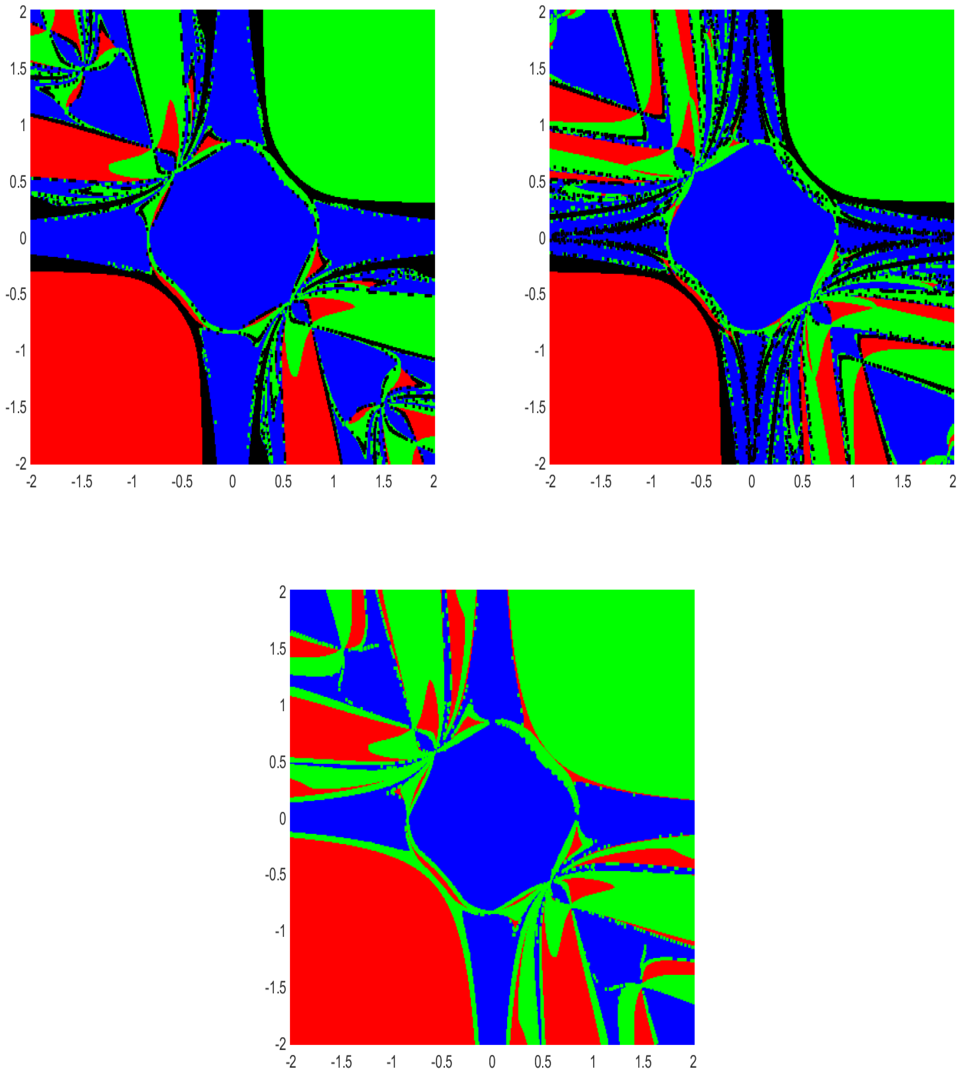
To obtain the convergence region of Methods (2), (3) and (4), we study the Basins of Attraction (BA) (i.e., the collection of all initial points from which the iterative method converges to a solution of a given equation) and Julia sets (JS) (i.e., the complement of basins of attraction) [18]. In fact, we study the BA associated with the roots of the three systems of equations given in Examples 5–7.

Example 5.

$\left\{\begin{array}{c}{s}_1^3-s_2=0\hfill \\ s_2^3-s_1=0.\hfill \end{array}\right.$

The solutions are $(-1,-1),(0,0)$ and $(1,1)$

Example 6.

$\left\{\begin{array}{c}3s_1^2{s}_2-s_2^3=0\hfill \\ s_1^3-3s_1{s}_2^2-1=0.\hfill \end{array}\right.$

The solutions are $(-\frac{1}{2},-\frac{\sqrt{3}}{2}),(-\frac{1}{2}$ and $\frac{\sqrt{3}}{2}),(1,0).$

Example 7.

$\left\{\begin{array}{c}{s}_1^2+s_2^2-4=0\hfill \\ 3s_1^2+7s_2^2-16=0.\hfill \end{array}\right.$

The solutions are $(\sqrt{3},1),(-\sqrt{3},1),(\sqrt{3},-1)$ and $(-\sqrt{3},-1).$

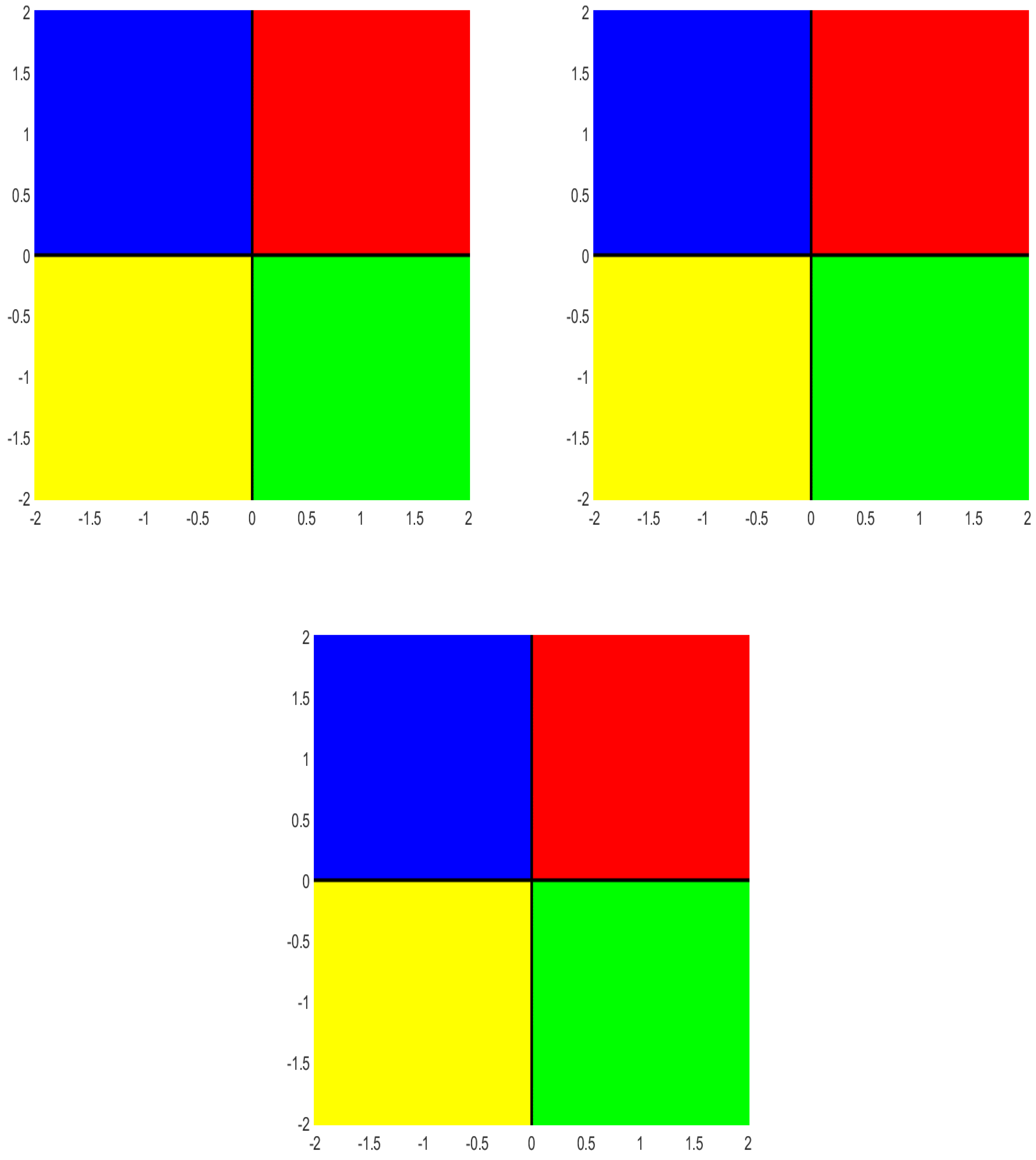
The region $\mathcal{R}=\{(x,y)\in {\mathbb{R}}^2:-2\le x\le 2,-2\le y\le 2\}$ which contains all the roots of Examples 5–7 is used to plot BA and JS. We choose an equidistant grid of $401\times 401$ points in $\mathcal{R}$ as the initial guess $x_0$, for Methods (2), (3) and (4). A tolerance level of ${10}^{-8}$ and a maximum of 50 iterations are used. A color is assigned to each attracting basin corresponding to each root, and if we do not obtain the desired tolerance with the fixed iterations, we assign the color black (i.e., we decide that the iterative method starting at $x_0$ does not converge to any of the roots). In this way, we distinguish each BA by their respective colors for the distinct roots of each method.

Figure 1, Figure 2 and Figure 3 demonstrate the BA corresponding to each root of the above examples (Examples 5–7) for Methods (2), (3) and (4). The JS (black region), which contains all the initial points from which the iterative method does not converge to any of the roots, can easily be observed in the figures.

Figure 1. Dynamics of (2), (3) and (4), respectively, with BA, for Example 5.

Figure 2. Dynamics of (2), (3) and (4), respectively, with BA, for Example 6.

Figure 3. Dynamics of (2), (3) and (4), respectively, with BA, for Example 7.

All the calculations in this paper were performed on a 16-core 64-bit Windows machine with Intel Core i7-10700 CPU @ 2.90GHz, using MATLAB.

In Figure 1 (corresponding to Example 5), the red region is the set of all initial points from which the iterates (2), (3) and (4) converge to $(-1,-1),$ the blue region is the set of all initial points from which the iterates (2), (3) and (4) converge to $(0,0)$ and the green region is the set of all initial points from which the iterates (2), (3) and (4) converge to $(1,1).$ The black region represents the Julia set.

In Figure 2 (corresponding to Example 6), the red region is the set of all initial points from which the iterates (2), (3) and (4) converge to $(-\frac{1}{2},-\frac{\sqrt{3}}{2}),$ the blue region is the set of all initial points from which the iterates (2), (3) and (4) converge to $(-\frac{1}{2},\frac{\sqrt{3}}{2})$ and the green region is the set of all initial points from which the iterates (2), (3) and (4) converge to $(1,0).$ The black region represents the Julia set.

In Figure 3 (corresponding to Example 7), the red region is the set of all initial points from which the iterates (2), (3) and (4) converge to $(\sqrt{3},1),$ the blue region is the set of all initial points from which the iterates (2), (3) and (4) converge to $(-\sqrt{3},1),$ the green region is the set of all initial points from which the iterates (2), (3) and (4) converge to $(\sqrt{3},-1)$ and the yellow region is the set of all initial points from which the iterates (2), (3) and (4) converge to $(-\sqrt{3},-1).$ The black region represents the Julia set.

8. Conclusions

In this article, Method (2) is extended to methods with better orders of convergence. The analyses of the local and semilocal convergence criteria for these methods, Methods (2), (3) and (4), are carried out with the assumptions imposed only on the first and second derivatives of the operator involved and without the application of Taylor series expansion. Additionally, the Fatou and Julia sets corresponding to these methods, including appropriate comparisons and examples, are displayed, thus verifying the theoretical approach.

References

1. Argyros, I.K. The Theory and Applications of Iteration Methods, 2nd ed.; Engineering Series; CRC Press, Taylor and Francis Group: Boca Raton, FL, USA, 2022. [Google Scholar]
2. Argyros, I.K.; Magréñan, A.A. A Contemporary Study of Iterative Schemes; Elsevier, Academic Press: New York, NY, USA, 2018. [Google Scholar]
3. Cordero, A.; Hueso, J.L.; Martínez, E.; Torregrosa, J.R. Increasing the convergence order of an iterative method for nonlinear systems. Appl. Math. Lett. 2012, 25, 2369–2374. [Google Scholar] [CrossRef]
4. Cordero, A.; Martínez, E.; Toregrossa, J.R. Iterative methods of order four and five for systems of nonlinear equations. J. Comput. Appl. Math. 2012, 231, 541–551. [Google Scholar] [CrossRef]
5. Magréñan, A.A.; Argyros, I.K.; Rainer, J.J.; Sicilia, J.A. Ball convergence of a sixth-order Newton-like method based on means under weak conditions. J. Math. Chem. 2018, 56, 2117–2131. [Google Scholar] [CrossRef]
6. Shakhno, S.M.; Gnatyshyn, O.P. On an iterative Method of order 1.839... for solving nonlinear least squares problems. Appl. Math. Applic. 2005, 161, 253–264. [Google Scholar]
7. Cordero, A.; Torregrosa, J.R. Variants of Newton’s method using fifth order quadrature formulas. Appl. Math. Comput. 2007, 190, 686–698. [Google Scholar] [CrossRef]
8. Darvishi, M.T.; Barati, A. A fourth-order method from quadrature formulae to solve systems of nonlinear equations. Appl. Math. Comput. 2007, 188, 257–261. [Google Scholar] [CrossRef]
9. Darvishi, M.T.; Barati, A. A third-order newton-type method to solve systems of nonlinear equations. Appl. Math. Comput. 2007, 187, 630–635. [Google Scholar] [CrossRef]
10. Frontini, M.; Sormani, E. Third-order methods from quadrature formulae for solving systems of nonlinear equations. Appl. Math. Comput. 2004, 149, 771–782. [Google Scholar] [CrossRef]
11. Homeier, H.H.H. A modified newton method with cubic convergence: The multivariable case. J. Comput. Appl. Math 2004, 169, 161–169. [Google Scholar] [CrossRef]
12. Khirallah, M.Q.; Hafiz, M.A. Novel three order methods for solving a system of nonlinear equations. Bull. Math. Sci. Appl. 2012, 2, 1–14. [Google Scholar] [CrossRef]
13. Noor, M.A.; Waseem, M. Some iterative methods for solving a system of nonlinear equations. J. Comput. Math. Appl. 2009, 57, 101–106. [Google Scholar] [CrossRef] [Green Version]
14. Podisuk, M.; Chundang, U.; Sanprasert, W. Single-step formulas and multi-step formulas of integration method for solving the initial value problem of ordinary differential equation. Appl. Math. Comput. 2007, 190, 1438–1444. [Google Scholar] [CrossRef]
15. Liu, Z.; Zheng, Q.; Huang, C. Third- and fifth-order Newton–Gauss methods for solving nonlinear equations with n variables. Appl. Math. Comput. 2016, 290, 250–257. [Google Scholar] [CrossRef]
16. Behl, R.; Maroju, P.; Martínez, E.; Singh, S. A study of the local convergence of a fifth order iterative scheme. Indian J. Pure Appl. Math. 2020, 51, 439–455. [Google Scholar]
17. Iliev, A.; Iliev, I. Numerical method with order t for solving system nonlinear equations. In Proceedings of the Collection of Works from the Scientific Conference Dedicated to 30 Years of FMI, Plovdiv, Bulgaria, 1–3 November 2000; pp. 105–112. [Google Scholar]
18. Magréñan, A.A.; Gutiérrez, J.M. Real dynamics for damped Newton’s method applied to cubic polynomials. J. Comput. Appl. Math. 2015, 275, 527–538. [Google Scholar] [CrossRef]
19. George, S.; Sadananda, R.; Jidesh, P.; Argyros, I.K. On the Order of Convergence of Noor-Waseem Method. Mathematics 2022, 10, 4544. [Google Scholar] [CrossRef]