RBF-Based Local Meshless Method for Fractional Diffusion Equations

Abstract

The fractional diffusion equation is one of the important recent models that can efficiently characterize various complex diffusion processes, such as in inhomogeneous or heterogeneous media or in porous media. This article provides a method for the numerical simulation of time-fractional diffusion equations. The proposed scheme combines the local meshless method based on a radial basis function (RBF) with Laplace transform. This scheme first implements the Laplace transform to reduce the given problem to a time-independent inhomogeneous problem in the Laplace domain, and then the RBF-based local meshless method is utilized to obtain the solution of the reduced problem in the Laplace domain. Finally, Stehfest’s method is utilized to convert the solution from the Laplace domain into the real domain. The proposed method uses Laplace transform to handle the fractional order derivative, which avoids the computation of a convolution integral in a fractional order derivative and overcomes the effect of time-stepping on stability and accuracy. The method is tested using four numerical examples. All the results demonstrate that the proposed method is easy to implement, accurate, efficient and has low computational costs.

1. Introduction

Fractional calculus (FC) has recently received much attention among the research community. Applications of FC can be found in a large number of phenomena, such as traffic models, stochastic systems, diffusion processes, earthquake design, and control processing, etc. [1,2,3]. The time-fractional order diffusion equations (TFDEs) have been shown to be very efficient at describing diffusion in complex systems [4,5]. The diffusion processes have been observed in various areas, for example, seepage in porous media [6], electron transportation [7], magmatic plasma [8], dissipation [9], and turbulence [10], etc.

Recently, TFDEs have attracted remarkable attention [11,12,13,14,15,16,17]. However, the analytic solution of TFDEs is rare, except for simple initial-boundary data [18]. Therefore, the numerical methods play a vital role in obtaining the solution of TFDEs. Numerous numerical techniques have been designed for the approximation of TFDEs. For example, Bayrak et al. [19] developed an efficient Chebyshev collocation technique for the simulations of TFDEs. In [20], the splines method was utilized for approximating the solution of TFDEs. Li et al. [21] utilized the Galerkin finite element method to study the solutions of TFDEs. In [22], the authors approximated the solution of variable order TFDEs. Bouchama et al. [23] proposed a finite difference method (FDM) for TFDEs. In [24], the others approximated the solution of TFDEs by using the Crank–Nicholson technique combined with spatial extrapolation. Other methods related to the study of the solutions of TFDEs can be found in [25,26] and their references.

On the other hand, the recently introduced meshless methods for the numerical approximation of the solution of PDEs are easy to use and have been applied to numerically simulate a large number of PDEs. The popularity of the meshless method stems from the ease with which the geometry of a problem can be established without the burden of constructing complex meshes. Meshless methods have received increasing attention for solving PDEs. For instance, the authors in [27], proposed the Galerkin method based on dual-Chebyshev wavelets to approximate the solution of 2nd-kind boundary integral equations. Assari et al. [28] developed a method based on logarithmic kernels to numerically simulate the $2D$ Fredholm integral equations of 2nd kind. The authors of [29] used the meshless local Petrov–Galerkin method to approximate the solution of time-dependent Maxwell equations. In [30], the authors obtained the numerical solution of non-linear integro-differential equations using the meshless method.

Another class of meshless methods, which are one of the best tools for the solution of PDEs, is RBF-based meshless methods [31]. RBF-based meshless methods have been applied to a large number of real-world problems. For example, the local multiquadric approximation methods were utilized in [32] for handling different boundary value problems. Jackson et al. [33] developed an adaptive RBF-based finite collocation approach for the simulation of diffusion problems. Naffa and Al-Gahtani [34] used the RBF-based meshless method for the solution of non-linear coupled differential equations. Leitao [35] used the RBF-based meshless method for $2D$ elastostatic problems. In [36], the authors developed a numerical-scheme-based RBF for solving stochastic advection–diffusion equations. All of these methods can be called global meshless methods. The main disadvantage of the global meshless methods is the ill-conditioned interpolation matrices that result from the discretization of the PDEs.

To overcome the drawback of global meshless methods, the RBF-based local meshless method was designed for diffusion problems [37]. Due to handiness, the RBF-based local meshless method has been applied to many complex problems, such as the generalized Gross–Pitaevskii equation [38], solid–liquid phase change problems  [39], singularly perturbed convection–diffusion–reaction equations [40], and fluid flow problems in Darcy porous media [41], etc. The main idea of the RBF-based local method is the collocation over local domains instead of the whole domain, which exceptionally reduces the size of the collocation matrix at the cost of solving small systems. The size of each small system is the number of nodes included in each local domain. The main drawback of RBF-based local meshless is that it does not work for elliptic problems in a straightforward way [42]. Furthermore, all of the mentioned methods use the FDM for temporal discretization, and these methods have a common shortcoming of time instability. The time-stepping technique is stable if the error decays or remains constant during computations. Furthermore, the optimal results are obtained for a very small time step, and hence, this method faces an increase in computational costs [43]. Therefore, to overcome the shortcomings associated with the FDM temporal discretization techniques, the Laplace transform has been used.

Laplace transform (LT) is one of the powerful tools used in the literature, coupled with other methods for the numerical modeling of PDEs. LT has been shown to be suitable for solving diffusion problems and can work efficiently as an alternative to the FDM [44]. However, in using the LT, the main difficulty is its inversion. Various methods are designed for the numerical inversion of LT. For the first time, LT was used in [45], coupled with a boundary integral equation method, and for inversion of the LT, Prony’s series of a negative exponential in time was used. In [46], the authors used the Fourier series method for the numerical inversion of LT. An efficient improvement in the Fourier series method was developed in [47]. Other numerical inversion methods for LT are the Crump method [48], the De Hoog method [49], the Weeks method [50], and others (see [51,52,53,54,55,56]). However, Stehfest’s method [57,58] is one of the simplest methods in implementation for numerical inverse LT. Davies and Martin [59] tested and evaluated a large number of inversion methods for LT, and they recommended Stehfest’s method because of its simplicity and acceptable accuracy. The goal of this work is to establish a numerical scheme coupling Laplace transform with an RBF-based local meshless method for the numerical simulation of multi-dimensional TFDEs. The Laplace transform is used to avoid the time stepping technique and possible stability restrictions in time. The RBF-based local meshless is used to overcome the dense and ill-conditioned RBF differentiation matrices.

The content of the paper is organized as follows. In Section 2, a brief description of the proposed numerical scheme is given. In Section 3, the stability of the numerical scheme is discussed. In Section 4, the numerical experiments are given. In Section 5, some conclusions are drawn.

2. Proposed Method

2.1. Time-Fractional Diffusion Equation

We consider a TFDE in a bounded domain $\mathrm{\Xi }$ and its boundary $\partial \mathrm{\Xi }$ of the form

$$D_t^{\alpha }u(\overline{\mathbf{\varsigma }},t)={\mathcal{L}}_{\mathcal{G}}u(\overline{\mathbf{\varsigma }},t)+\mathcal{Q}(\overline{\mathbf{\varsigma }},t),0<\alpha <1,\overline{\mathbf{\varsigma }}\in \mathrm{\Xi },t\in (0,T),$$

(1)

with boundary conditions

$${\mathcal{L}}_{\mathcal{B}}u(\overline{\mathbf{\varsigma }},t)=\mathcal{B}(\overline{\mathbf{\varsigma }},t),\overline{\mathbf{\varsigma }}\in \partial \mathrm{\Xi },t\in (0,T),$$

(2)

and initial condition

$$u(\overline{\mathbf{\varsigma }},0)=u_0\left(\overline{\mathbf{\varsigma }}\right),\overline{\mathbf{\varsigma }}\in \mathrm{\Xi },$$

(3)

where ${\mathcal{L}}_{\mathcal{G}}=D\mathrm{\Delta }+\overrightarrow{V}•\nabla -k$ and ${\mathcal{L}}_{\mathcal{B}}$ are the governing and boundary operators, $\mathcal{Q}(\overline{\mathbf{\varsigma }},t),$$\mathcal{B}(\overline{\mathbf{\varsigma }},t),u_0\left(\overline{\mathbf{\varsigma }}\right)$ are given functions; $\overline{\mathbf{\varsigma }}=(x,y)$ for 2D and $\overline{\mathbf{\varsigma }}=(x,y,z)$ for 3D, $\overrightarrow{V}$ the velocity vector, D and k are the diffusion and reaction coefficients, T the final time and $D_t^{\alpha }$ denotes the Liouville–Caputo fractional derivative defined as

$$D_t^{\alpha }u(\overline{\mathbf{\varsigma }},t)=\frac{1}{\mathrm{\Gamma }(1-\alpha )}{\int }_0^t\frac{\partial u(\overline{\mathbf{\varsigma }},\tau )}{\partial \tau }\frac{d\tau }{{(t-\tau )}^{\alpha }},0<\alpha \le 1.$$

(4)

2.2. Implementation of the Proposed Method

Figure 1 shows the flow chart of the proposed method. The proposed method has three major steps: (i) Laplace transform; (ii) RBF-based local meshless method; (iii) Stehfest method.

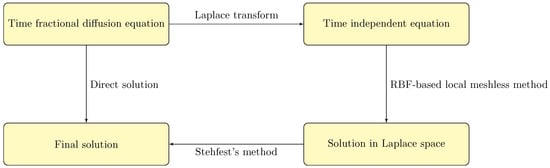
Figure 1. The flowchart of the proposed method.

2.2.1. (i) Laplace Transform

In the first step, the Laplace transform is used to convert the time-fractional diffusion equation from the time domain to the Laplace domain. The LT of the function $u(\overline{\mathbf{\varsigma }},t)$, is denoted by $\widehat{u}(\overline{\mathbf{\varsigma }},s)$ and is defined as

$$\widehat{u}(\overline{\mathbf{\varsigma }},s)={\int }_0^{\infty }{e}^{-st}u(\overline{\mathbf{\varsigma }},t)dt,$$

(5)

and the LT of $D_t^{\alpha }u(\overline{\mathbf{\varsigma }},t)$ is defined as

$$\mathcal{L}\left\{D_t^{\alpha }u(\overline{\mathbf{\varsigma }},t)\right\}=s^{\alpha }\widehat{u}(\overline{\mathbf{\varsigma }},s)-s^{\alpha -1}{u}_0.$$

(6)

Applying LT to (1) and (2) gives

$$s^{\alpha }\widehat{u}(\overline{\mathbf{\varsigma }},s)-s^{\alpha -1}{u}_0={\mathcal{L}}_{\mathcal{G}}\widehat{u}(\overline{\mathbf{\varsigma }},s)+\widehat{\mathcal{Q}}(\overline{\mathbf{\varsigma }},s),$$

(7)

and

$${\mathcal{L}}_{\mathcal{B}}\widehat{u}(\overline{\mathbf{\varsigma }},s)=\widehat{\mathcal{B}}(\overline{\mathbf{\varsigma }},s),$$

(8)

Equations (7) and (8) imply

$$(s^{\alpha }I-{\mathcal{L}}_{\mathcal{G}})\widehat{u}(\overline{\mathbf{\varsigma }},s)=\widehat{G_1}(\overline{\mathbf{\varsigma }},s),$$

(9)

and

$${\mathcal{L}}_{\mathcal{B}}\widehat{u}(\overline{\mathbf{\varsigma }},s)=\widehat{\mathcal{B}}(\overline{\mathbf{\varsigma }},s).$$

(10)

where

$$\widehat{G_1}(\overline{\mathbf{\varsigma }},s)=s^{\alpha -1}{u}_0+\widehat{\mathcal{Q}}(\overline{\mathbf{\varsigma }},s).$$

where I is the identity operator, ${\mathcal{L}}_{\mathcal{G}}$ is the linear differential operator, and ${\mathcal{L}}_{\mathcal{B}}$ is the boundary differential operator. Here, we need to solve the system defined in (9) and (10) for every point s in the LT domain. For this, first we discretize the operators ${\mathcal{L}}_{\mathcal{G}}$ and ${\mathcal{L}}_{\mathcal{B}}$ using the RBF-based local meshless method. Then, the system is solved for each point s in the LT domain. Finally, the solution to the problem defined in Equations (1)–(3) is obtained using Stehfest’s method. The RBF-based local meshless method is discussed in the following section.

2.2.2. (ii) RBF-Based Local Meshless Method

In the RBF-based local meshless method for a given set ${\left\{\widehat{u}\left({\overline{\mathbf{\varsigma }}}_i\right)\right\}}_{i=1}^{{\mathcal{G}}_N}$, where ${\left\{{\overline{\mathbf{\varsigma }}}_i\right\}}_{i=1}^{{\mathcal{G}}_N}\subset \mathrm{\Xi }$,  the function $\widehat{u}\left(\overline{\mathbf{\varsigma }}\right)$ has an approximation given as,

$$\widehat{u}\left({\overline{\mathbf{\varsigma }}}_i\right)=\sum _{{\overline{\mathbf{\varsigma }}}_j\in {\mathrm{\Xi }}_i}{\alpha }_j^i\varphi (\parallel {\overline{\mathbf{\varsigma }}}_i-{\overline{\mathbf{\varsigma }}}_j^i\parallel ),$$

(11)

where ${\mathbf{\alpha }}^i={\left\{{\alpha }_j^i\right\}}_{j=1}^n$ denotes the unknwon coefficients, and  $\varphi \left(r\right),r>0$ is a kernel function. ${\mathrm{\Xi }}_i$ is the local domain, and $\mathrm{\Xi }$ is the global domain. ${\mathrm{\Xi }}_i$ contain the point ${\overline{\mathbf{\varsigma }}}_i$ and ${\sigma }_n$ neighboring points. Thus, we have ${\mathcal{G}}_N$ number of ${\sigma }_n\times {\sigma }_n$ small size systems given as

$$\left(\begin{array}{c}\widehat{u}\left({\overline{\mathbf{\varsigma }}}_1^i\right)\\ \widehat{u}\left({\overline{\mathbf{\varsigma }}}_2^i\right)\\ .\\ .\\ .\\ \widehat{u}\left({\overline{\mathbf{\varsigma }}}_{{\sigma }_n}^i\right)\end{array}\right)=\left(\begin{array}{cccccc}\varphi (\parallel {\overline{\mathbf{\varsigma }}}_1^i-{\overline{\mathbf{\varsigma }}}_1^i\parallel )& \varphi (\parallel {\overline{\mathbf{\varsigma }}}_1^i-{\overline{\mathbf{\varsigma }}}_2^i\parallel )& .& .& .& \varphi (\parallel {\overline{\mathbf{\varsigma }}}_1^i-{\overline{\mathbf{\varsigma }}}_{{\sigma }_n}^i\parallel )\\ \varphi (\parallel {\overline{\mathbf{\varsigma }}}_2^i-{\overline{\mathbf{\varsigma }}}_1^i\parallel )& \varphi (\parallel {\overline{\mathbf{\varsigma }}}_2^i-{\overline{\mathbf{\varsigma }}}_2^i\parallel )& .& .& .& \varphi (\parallel {\overline{\mathbf{\varsigma }}}_2^i-{\overline{\mathbf{\varsigma }}}_{{\sigma }_n}^i\parallel )\\ .& .& & .& & .\\ .& .& & .& & .\\ .& .& & .& & .\\ \varphi (\parallel {\overline{\mathbf{\varsigma }}}_{{\sigma }_n}^i-{\overline{\mathbf{\varsigma }}}_1^i\parallel )& \varphi (\parallel {\overline{\mathbf{\varsigma }}}_n^i-{\overline{\mathbf{\varsigma }}}_2^i\parallel )& .& .& .& \varphi (\parallel {\overline{\mathbf{\varsigma }}}_{{\sigma }_n}^i-{\overline{\mathbf{\varsigma }}}_{{\sigma }_n}^i\parallel )\end{array}\right)\left(\begin{array}{c}{\alpha }_1^i\\ {\alpha }_2^i\\ .\\ .\\ .\\ {\alpha }_{{\sigma }_n}^i\end{array}\right),i=1,2,3,\dots ,{\mathcal{G}}_N,$$

(12)

which implies,

$${\widehat{\mathbf{u}}}^i={\mathrm{\Phi }}^i{\mathbf{\alpha }}^i,i=1,2,3,\dots ,{\mathcal{G}}_N,$$

(13)

the entries of the interpolation matrix ${\mathrm{\Phi }}^i$ are of the form $b_{kj}^i=\varphi (\parallel {\overline{\mathbf{\varsigma }}}_k^i-{\overline{\mathbf{\varsigma }}}_j^i\parallel ),\mathrm{where}{\overline{\mathbf{\varsigma }}}_k^i,{\overline{\mathbf{\varsigma }}}_j^i\in {\mathrm{\Xi }}_i$. For the differential operator ${\mathcal{L}}_{\mathcal{G}}$ we have,

$${\mathcal{L}}_{\mathcal{G}}\widehat{u}\left({\overline{\mathbf{\varsigma }}}_i\right)=\sum _{{\overline{\mathbf{\varsigma }}}_j\in {\mathrm{\Xi }}_i}{\mathbf{\alpha }}_j^i{\mathcal{L}}_{\mathcal{G}}\varphi (\parallel {\overline{\mathbf{\varsigma }}}_i-{\overline{\mathbf{\varsigma }}}_j^i\parallel ),$$

(14)

From Equation (14), we have

$${\mathcal{L}}_{\mathcal{G}}\widehat{u}\left({\overline{\mathbf{\varsigma }}}_i\right)={\mathbf{\nu }}^i·{\mathbf{\alpha }}^i,$$

(15)

where ${\mathbf{\alpha }}^i$ and ${\mathbf{\nu }}^i$ are column and row vectors of order ${\sigma }_n$. Elements of ${\mathbf{\nu }}^i$ are of the form

$${\mathbf{\nu }}^i={\mathcal{L}}_{\mathcal{G}}\varphi (\parallel {\overline{\mathbf{\varsigma }}}_i-{\overline{\mathbf{\varsigma }}}_j^i\parallel ),{\overline{\mathbf{\varsigma }}}_j^i\in {\mathrm{\Xi }}_i,$$

(16)

From Equation (13), we have,

$${\mathbf{\alpha }}^i={\left({\mathrm{\Phi }}^i\right)}^{-1}{\widehat{\mathbf{u}}}^i,$$

(17)

From (17) and (15), we have

$$\begin{array}{cc}\hfill {\mathcal{L}}_{\mathcal{G}}\widehat{u}\left({\overline{\mathbf{\varsigma }}}_i\right)=& {\mathbf{\nu }}^i{\left({\mathrm{\Phi }}^i\right)}^{-1}{\widehat{\mathbf{u}}}^i\hfill \\ \hfill =& {\mathbf{fi}}^i{\widehat{\mathbf{u}}}^i,\hfill \end{array}$$

(18)

where,

$${\mathbf{\beta }}^i={\mathbf{\nu }}^i{\left({\mathrm{\Phi }}^i\right)}^{-1},$$

(19)

thus, the local radial basis function approximation of the operator ${\mathcal{L}}_{\mathcal{G}}$ at each point ${\overline{\mathbf{\varsigma }}}_i$ is given as

$${\mathcal{L}}_{\mathcal{G}}\widehat{u}\equiv \mathcal{D}\widehat{\mathbf{u}},$$

(20)

where ${\mathcal{D}}_{{\mathcal{G}}_N\times {\mathcal{G}}_N}$ is a sparse matrix approximating ${\mathcal{L}}_{\mathcal{G}}$. The operator ${\mathcal{L}}_{\mathcal{B}}$ can also be approximated in a similar way.

2.2.3. Selection of Best Shape Parameter

We have utilized the multiquadric radial basis kernel function (MQ-RBF) $\varphi (r,\vartheta )$ = $\sqrt{1+{\left(\vartheta r\right)}^2}$ in our experiments. This MQ-RBF contains the parameter $\vartheta$; for the accuracy of the numerical solution, the value of the parameter $\vartheta$ is varied. To condition number $\mathcal{N}$ of the matrix, ${\mathrm{\Phi }}^i$ is utilized to quantify the sensitivity to perturbation of the linear system. In this work, the uncertainty principle [60] is used to obtain the best value of the shape parameter $\vartheta$. A pseudo code of this algorithm is represented in Algorithm 1.

Algorithm 1 Optimal Shape Parameter.

Step 1: set $\mathcal{N}=1$ Step 2: select ${10}^{+12}<\mathcal{N}<{10}^{+16}$ Step 3: while $\mathcal{N}>{\mathcal{N}}_{max}$ and $\mathcal{N}<{\mathcal{N}}_{min}$ Step 4: Construct the matrix ${\mathrm{\Phi }}^i$ Step 4: $\mathit{E},\mathit{S},\mathit{P}=svd\left({\mathrm{\Phi }}^i\right)$ Step 5: $\mathcal{N}=\frac{{\rho }_{max}}{{\rho }_{min}}$ Step 6: if $\mathcal{N}<{\mathcal{N}}_{min},\vartheta =\vartheta -\delta \vartheta$ Step 7: if $\mathcal{N}>{\mathcal{N}}_{max},\vartheta =\vartheta +\delta \vartheta$ $\vartheta$ (optimal) = $\vartheta$.

Where ${\mathit{E}}_{{\sigma }_n\times {\sigma }_n},$${\mathit{P}}_{{\sigma }_n\times {\sigma }_n}$ are the orthogonal matrices, and ${\mathit{S}}_{{\sigma }_n\times {\sigma }_n}$ is the diagonal matrix containing the singular values of the matrix ${\mathrm{\Phi }}^i$. ${\rho }_{max}$, ${\rho }_{min}$ are the maximum and minimum singular values of the matrix ${\mathrm{\Phi }}^i$, and $\delta \vartheta$ is the increment of $\vartheta$. After obtaining the best value of the shape parameter, we compute ${\left({\mathrm{\Phi }}^i\right)}^{-1}$ using the svd as ${\left({\mathrm{\Phi }}^i\right)}^{-1}={\left({\mathbf{ESP}}^{\mathbf{T}}\right)}^{-1}={\mathbf{PS}}^{-\mathbf{1}}{\mathbf{E}}^{\mathbf{T}}$ (see [61]). Hence, we can calculate $\mathbf{\beta }$${}^i$ in (19).

2.2.4. (iii) Numerical Approximation of Inverse Laplace Transform via Stehfest’s Method

This section is devoted to the numerical approximation of inverse LT. Here we implement Stehfest’s algorithm for this purpose. Stehfest’s method is one of the most important methods used for an approximation of the inverse LT. Due to its simplicity and efficiency, it is becoming popular in many areas such as economics, geophysics, financial mathematics, chemistry and computational physics. It has a fast convergence rate, and for smooth functions, it gives accurate approximations. The solution using this algorithm is obtained as

$$u_{app}(\overline{\mathbf{\varsigma }},t)=\frac{ln2}{t}\sum _{k=1}^{N_S}{\zeta }_k\widehat{u}(\overline{\mathbf{\varsigma }},s_k),$$

(21)

where the weights ${\zeta }_k$ are given by

$${\zeta }_k={(-1)}^{\frac{N_S}{2}+k}\sum _{l=\lfloor \frac{k+1}{2}\rfloor }^{min(k,\frac{N_S}{2})}\frac{l^{\frac{N_S}{2}}(2l!)}{(\frac{N_S}{2}-l)!l!(l-1)!(k-l)!(2l-k)!}.$$

(22)

Stehfest’s number $N_S$ should be even. The system (9) and (10) is solved for $s_k=\frac{ln2}{t}k$, $k=1,2,3,\dots ,N_S$ in LT space. Finally, the solution is obtained using (21). This method has some interesting features: (i) using the Stehfest algorithm, linear approximations in values of the transform function are obtained; (ii) the coefficients can be easily calculated; (ii) we require the values of the transform function for real s only; (iv) for constant functions, the method produces almost exact results. Many authors have studied Stehfest’s method [59,62], where it has been reported that for non-oscillatory functions, this algorithm has very fast convergence.

2.3. Error Analysis

This section is about the error analysis of the proposed numerical method. Our method is based on three main steps. In the first step, the LT is used in which no error occurs. In the second step, the RBF-based local meshless method is used, which has an error estimate of order $O\left({\varrho }^{\frac{1}{\vartheta F_d}}\right),0<\varrho <1,$ where $F_d$ and $\vartheta$ denote the fill distance and shape parameter [31]. Finally, the numerical inversion LT is approximated using Stehfest’s method. The authors of [63,64] have discussed the error analysis of this method. They have studied the effect of the involved parameters on the efficiency and numerical accuracy of the method. They concluded their finding as “If $\xi$ significant digits are required, let for a positive integer $N_S=\lceil 2.2\xi \rceil$. Set the system’s precision at $\gamma =\lceil 1.1N_S\rceil$. Then, for t and $\widehat{u}(\overline{\mathbf{\varsigma }},s)$, compute $u(\overline{\mathbf{\varsigma }},t)$ in (21)”. According to these observations, we have the error estimate given as follows.

Remark 1

([65]). If the error is ${10}^{-(\gamma +1)}\le \frac{\parallel \widehat{u}-u\parallel }{\parallel u\parallel }\le {10}^{-\gamma }$, via $\gamma =\lceil 1.1N_S\rceil$. Then, the error is ${10}^{-(\xi +)1}\le \frac{\parallel \widehat{u}-u\parallel }{\parallel u\parallel }\le {10}^{-\xi }$, where $N_S=\lceil 2.2\xi \rceil .$

The sufficient conditions on the function $u(\overline{\mathbf{\varsigma }},t)$, which ensures the convergence of $u_{app}(\overline{\mathbf{\varsigma }},t)$ are presented in the next theorem.

Theorem 1

([62]). Assume $u\left(t\right):(0,\infty )\to \mathbb{R}$ is a locally integrable function, such that its Laplace transform $\widehat{u}\left(s\right)$ exists for all $s>0,$ and that $u_{app}\left(t\right)$ is defined by (21).

1. 

The convergence of $u_{app}\left(t\right)$ depends only on the values of $u\left(t\right)$ in the neighborhood of t.

2. 

Assume that for some $m\in \mathbb{R}$ and some $\epsilon \in (0,1/4)$

$${\int }_0^{\epsilon }|u(-tlo{g}_2(1/2+\nu ))+u(-tlo{g}_2(1/2-\nu ))-2m|{\nu }^{-1}d\nu <\infty .$$

Then $u_{app}\left(t\right)\to m$ as $N_S\to +\infty .$

3. 

Assume that the function has bounded variation in the neighborhood of $t.$ Then

$$u_{app}\left(t\right)\to \frac{u(t+0)+u(t-0)}{2}as{N}_S\to +\infty .$$

Corollary 1.

Under the assumptions of the above theorem, if

$$u(t+\nu )-u\left(t\right)=O\left({\left|\nu \right|}^{\upsilon }\right)$$

$\forall \nu$ and some υ in the neighborhood of $t,$ then $u_{app}\left(t\right)\to u\left(t\right),$ as $N_S\to +\infty .$

3. Stability

Here we discuss the stability of the fully discrete system (9) and (10). We write the system in the following form

$$\mathcal{A}\widehat{\mathit{u}}=\mathit{q},$$

(23)

where the matrix A is obtained via an RBF-based local meshless method. The stability-constant denoted by $\eta$ for the system (23) is defined as

$$\eta =\underset{\widehat{\mathit{u}}\ne 0}{sup}\frac{\parallel \widehat{\mathit{u}}\parallel }{\parallel \mathcal{A}\widehat{\mathit{u}}\parallel },$$

(24)

the constant $\eta$ has finite value for any discrete norm $\parallel .\parallel$ on ${\mathbb{R}}^{{\mathcal{G}}_N}$. From Equation (24), we obtain

$${\parallel \mathcal{A}\parallel }^{-1}\le \frac{\parallel \widehat{\mathit{u}}\parallel }{\parallel \mathcal{A}\widehat{\mathit{u}}\parallel }\le \eta .$$

(25)

Furthermore, we can write

$$\parallel {\mathcal{A}}^{†}\parallel =\underset{\mathit{v}\ne 0}{sup}\frac{\parallel {\mathcal{A}}^{†}\mathit{v}\parallel }{\parallel \mathit{v}\parallel }.$$

(26)

where ${\mathcal{A}}^{†}$ is the pseudoinverse of $\mathcal{A}.$ Therefore,

$$\parallel {\mathcal{A}}^{†}\parallel \ge \underset{\mathit{v}=\mathcal{A}\widehat{\mathit{u}}\ne 0}{sup}\frac{\parallel {\mathcal{A}}^{†}\mathcal{A}\widehat{\mathit{u}}\parallel }{\parallel \mathcal{A}\widehat{\mathit{u}}\parallel }=\underset{\widehat{\mathit{u}}\ne 0}{sup}\frac{\parallel \widehat{\mathit{u}}\parallel }{\parallel \mathcal{A}\widehat{\mathit{u}}\parallel }=\eta .$$

(27)

Equations (25) and (26) give the bounds for the constant $\eta$. For (23), it may be difficult to compute the pseudoinverse, but the stability is guaranteed. MATLAB’s function “condest” can be used for evaluating $\parallel {\mathcal{A}}^{-1}{\parallel }_{\infty }$ as

$$\eta =\frac{condest\left({\mathcal{A}}^{\prime }\right)}{{\parallel \mathcal{A}\parallel }_{\infty }}$$

(28)

For the sparse differentiation matrix $\mathcal{A}$, this technique works well with less computational time. The bounds for the stability-constant $\eta$ of the system defined in (9) and (10) with ${\mathcal{G}}_N=150,N_S=20,\alpha =0.85,{\sigma }_n=25$ at $T=1$ for problem 1 are shown in Figure 2a, for problem 2 with ${\mathcal{G}}_N=625,N_S=18,\alpha =0.85,{\sigma }_n=20$ at $T=1$ are shown in Figure 2b, and for problem 4 with ${\mathcal{G}}_N=4913,N_S=18,\alpha =0.90,{\sigma }_n=80$ at $T=1$ are shown in Figure 2c. We can see that the constant $\eta$ is bounded by very small numbers, which confirms that the proposed RBF-based local meshless scheme is stable.

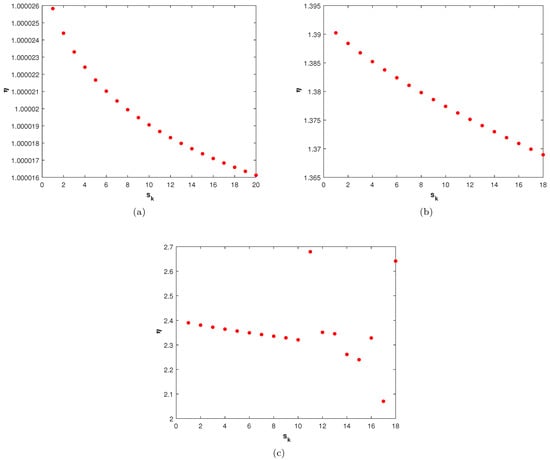
Figure 2. The plot shows the stability constant $\eta$ of the differentiation matrix $\mathcal{A}$ for (a) problem 1; (b) problem 2; (c) problem 4.

4. Numerical Results and Discussion

This section is devoted to numerical results and discussions. The performance, efficiency, accuracy and convergence of the RBF-based local meshless method is tested and validated using four test problems. Three error norms are used: the maximum absolute error, and the root mean square, and the relative error, which are denoted and defined below as

$$A{b}_{Error}=\underset{1\le j\le {\mathcal{G}}_N}{max}|u({\overline{\mathbf{\varsigma }}}_j,t)-u_{app}({\overline{\mathbf{\varsigma }}}_j,t)|,$$

$$Rm{s}_{Error}=\sqrt{\frac{{\sum }_{j=1}^{{\mathcal{G}}_N}{(u({\overline{\mathbf{\varsigma }}}_j,t)-u_{app}({\overline{\mathbf{\varsigma }}}_j,t))}^2}{{\mathcal{G}}_N}},$$

$$Re{l}_{Error}=\sqrt{\frac{{\sum }_{j=1}^{{\mathcal{G}}_N}{(u({\overline{\mathbf{\varsigma }}}_j,t)-u_{app}({\overline{\mathbf{\varsigma }}}_j,t))}^2}{{\sum }_{j=1}^{{\mathcal{G}}_N}{\left(u({\overline{\mathbf{\varsigma }}}_j,t)\right)}^2}}.$$

where $u({\overline{\mathbf{\varsigma }}}_j,t)$ and $u_{app}({\overline{\mathbf{\varsigma }}}_j,t)$ denote the analytic and numerical solutions. ${\mathcal{G}}_N$ and ${\sigma }_n$ are the nodes in the global and local domains, respectively, $N_S$ is the Stehfest number, and T is the final time.

4.1. Problem 1

In our first experiment, we consider a $1D$ TFDEs with Dirichlet boundary conditions in a domain $\mathrm{\Xi }=[0,2].$ The parameters in Equations (1)–(3) are chosen as $D=k=1,$ $\overrightarrow{\mathit{V}}=0,$$\mathcal{Q}(\overline{\mathbf{\varsigma }},t)=\left[\frac{2x(2-x)t^{2-\alpha }}{\mathrm{\Gamma }(3-\alpha )}+x(2-x)t^2+2t^2\right],$ $\mathcal{B}(\overline{\mathbf{\varsigma }},t)=0,$ $u_0\left(\overline{\mathbf{\varsigma }}\right)=0,$$\alpha =0.85$, and the analytic solution of the problem is $u(\overline{\mathbf{\varsigma }},t)=t^2\left(x(2-x)\right),$ in which $\overline{\mathbf{\varsigma }}=x\in \mathrm{\Xi }$. Table 1 presents the numerical accuracy of the proposed method using different values of $N_S,{\sigma }_n,{\mathcal{G}}_N,\alpha =0.85$ at final time $T=1.$ The numerical solutions at different time moments are shown in Figure 3. The space–time plot of the numerical solution of problem 1 is depicted in Figure 4a. The space-time plots of $A{b}_{Error}$ and $Rm{s}_{Error}$ are shown in Figure 4b and Figure 5, respectively. Figure 6a shows a comparison of the three error norms for various values of t with $N_S=18.$ Figure 6b shows a comparison of the three error norms for various values of $N_S$ at final time $T=1,$ and it is observed that the errors tend to decrease up to $N_S=18$ and then increase with an increase in $N_S$. From the results presented in Table 1 and Figure 3, Figure 4, Figure 5 and Figure 6, it is observed that the proposed method has produced accurate and stable results.

Table 1. The errors obtained using the proposed numerical scheme at final time $T=1$ corresponding to problem 1.

$\mathit{\alpha }=0.85$	${\mathcal{G}}_{\mathit{N}}$	${\mathit{\sigma }}_{\mathit{n}}$	${\mathit{N}}_{\mathit{S}}$	${\mathit{Ab}}_{\mathit{Error}}$	${\mathit{Rms}}_{\mathit{Error}}$	${\mathit{Rel}}_{\mathit{Error}}$	CPU(s)
	140	20	18	4.4420$\times {10}^{-4}$	3.7542$\times {10}^{-5}$	5.1591$\times {10}^{-5}$	0.101494
	145			2.0215$\times {10}^{-4}$	1.6787$\times {10}^{-5}$	2.3067$\times {10}^{-5}$	0.087209
	150			1.6953$\times {10}^{-4}$	1.3842$\times {10}^{-5}$	1.9018$\times {10}^{-5}$	0.102077
	150	25	16	1.6953$\times {10}^{-4}$	1.3842$\times {10}^{-5}$	1.9018$\times {10}^{-5}$	0.083023
		26		1.5566$\times {10}^{-4}$	1.2710$\times {10}^{-5}$	1.7462$\times {10}^{-5}$	0.092403
		29		1.2755$\times {10}^{-4}$	1.0414$\times {10}^{-5}$	1.4308$\times {10}^{-5}$	0.095714
	100	6	8	3.0429$\times {10}^{-2}$	3.0429$\times {10}^{-3}$	4.1876$\times {10}^{-3}$	0.072115
			10	1.9506$\times {10}^{-4}$	1.9506$\times {10}^{-5}$	2.6845$\times {10}^{-5}$	0.069145
			12	1.1745$\times {10}^{-4}$	1.1745$\times {10}^{-5}$	1.6163$\times {10}^{-5}$	0.083798
[66]				1.7$\times {10}^{-4}$

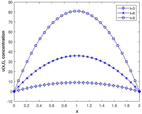
Figure 3. The concentration at different times.

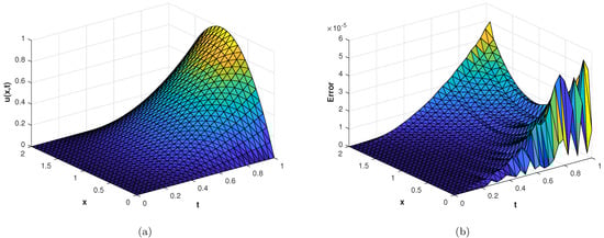
Figure 4. (a) Numerical solution of problem 1. (b) $A{b}_{Error}$ of the proposed method with ${\mathcal{G}}_N=30$, $N_S=18,{\sigma }_n=25$ at $T=1$ corresponding to problem 1.

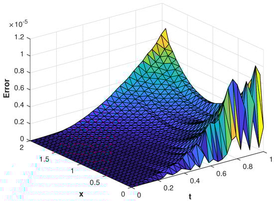
Figure 5. $Rm{s}_{Error}$ of the proposed method with ${\mathcal{G}}_N=30$, $N_S=18,{\sigma }_n=25$ at $T=1$ corresponding to problem 1.

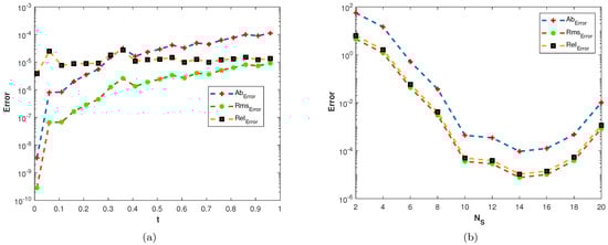
Figure 6. (a) Plots of $A{b}_{Error}$, $Rm{s}_{Error}$, and $Re{l}_{Error}$ versus t with ${\mathcal{G}}_N=150,{\sigma }_n=20,N_S=18$. (b) Plots of $A{b}_{Error}$, $Rm{s}_{Error}$, and $Re{l}_{Error}$ versus $N_S$ with ${\mathcal{G}}_N=150,{\sigma }_n=20,T=1$.

4.2. Problem 2

In our second experiment, we consider a $2D$ TFDE with Dirichlet boundary conditions in a domain $\mathrm{\Xi }={[0,1]}^2.$ The parameters in Equations (1)–(3) are chosen as $D=1,k=0,$ $\overrightarrow{\mathit{V}}=[0,0],$$\mathcal{Q}(\overline{\mathbf{\varsigma }},t)=\left[\frac{2t^{2-\alpha }}{3-\alpha }-2t^2\right]e^{(x+y)},$ $\mathcal{B}(\overline{\mathbf{\varsigma }},t)=t^2{e}^{(x+y)},$ $u_0\left(\overline{\mathbf{\varsigma }}\right)=0,$ $\alpha =0.85$, and the analytic solution of the problem is $u(\overline{\mathbf{\varsigma }},t)=t^2{e}^{(x+y)},$ in which $\overline{\mathbf{\varsigma }}=(x,y)\in \mathrm{\Xi }.$ The $A{b}_{Error},$ $Rm{s}_{Error}$ and $Re{l}_{Error}$ errors of the proposed method for problem 2 are presented in Table 2. The results are obtained using different values of $N_S,{\sigma }_n,{\mathcal{G}}_N$ and $\alpha =0.85.$ The numerical solution of problem 2 is shown in Figure 7a. The plots of $A{b}_{Error}$ and $Rm{s}_{Error}$ are shown in Figure 7b and Figure 8 computed using ${\mathcal{G}}_N=625,N_S=18,{\sigma }_n=20$ at final time $T=1.$ In Figure 9a,b, the plots show a comparison of the three error norms for various values of $N_S$ at $T=1$ and $T=0.01,$ we note that the errors tend to decrease up to $N_S=18$ and then increase with an increase in $N_S$. From the results, one can observe that Stehfest’s method gives optimal results for a value of $N_S$ up to $18.$ Figure 9c shows a comparison of the three error norms for different values of t, which shows that the method has produced stable results. In Figure 10 and Figure 11, the contour plots of $A{b}_{Error}$, and $Rm{s}_{Error}$ are depicted. From the obtained results, it is evident that the proposed scheme has produced results with acceptable accuracy.

Table 2. The errors obtained using the proposed scheme at final time $T=1$ for problem 2.

$\mathit{\alpha }=0.85$	${\mathit{\sigma }}_{\mathit{n}}$	${\mathit{Ab}}_{\mathit{Error}}$	${\mathit{Rms}}_{\mathit{Error}}$	${\mathit{Rel}}_{\mathit{Error}}$	CPU(s)
	15	4.88$\times {10}^{-1}$	2.44$\times {10}^{-2}$	7.50$\times {10}^{-3}$	4.069811
$({\mathcal{G}}_N,N_S)=(400,10)$	16	1.34$\times {10}^{-2}$	6.68$\times {10}^{-4}$	2.05$\times {10}^{-4}$	0.937441
	17	7.80$\times {10}^{-3}$	3.87$\times {10}^{-4}$	1.19$\times {10}^{-4}$	0.785719
	18	5.60$\times {10}^{-3}$	2.81$\times {10}^{-4}$	8.68$\times {10}^{-5}$	0.741108
	$N_S$
	10	2.70$\times {10}^{-3}$	1.09$\times {10}^{-4}$	3.39$\times {10}^{-5}$	1.635850
$({\mathcal{G}}_N,{\sigma }_n)=(625,25)$	12	2.22$\times {10}^{-3}$	8.68$\times {10}^{-5}$	2.68$\times {10}^{-5}$	1.221204
	14	2.28$\times {10}^{-3}$	1.13$\times {10}^{-4}$	3.49$\times {10}^{-5}$	1.309271
	16	3.00$\times {10}^{-3}$	1.21$\times {10}^{-4}$	3.76$\times {10}^{-5}$	1.231612
	18	3.20$\times {10}^{-3}$	1.27$\times {10}^{-4}$	3.94$\times {10}^{-5}$	1.309295
	20	8.20$\times {10}^{-4}$	3.28$\times {10}^{-5}$	1.01$\times {10}^{-5}$	1.418298
[67]		1.140$\times {10}^{-3}$

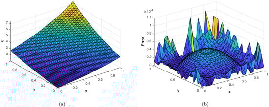
Figure 7. (a) Numerical solution of problem 2. (b) $A{b}_{Error}$ of the proposed method computed using ${\mathcal{G}}_N=625,N_S=18,{\sigma }_n=20$ at $T=1$ corresponding to problem 2.

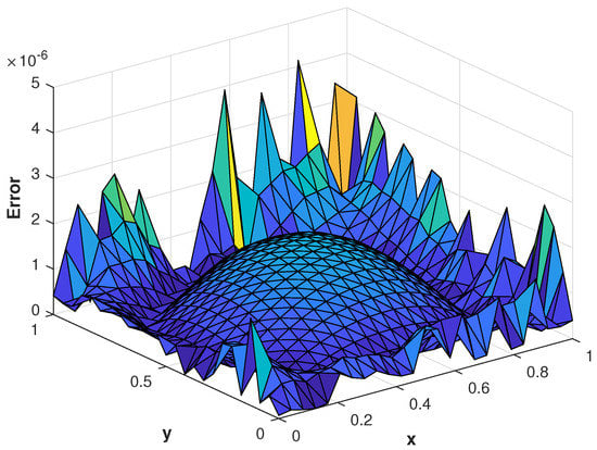
Figure 8. $Rm{s}_{Error}$ of the proposed method computed using ${\mathcal{G}}_N=625,N_S=18,{\sigma }_n=20$ at $T=1$ corresponding to problem 2.

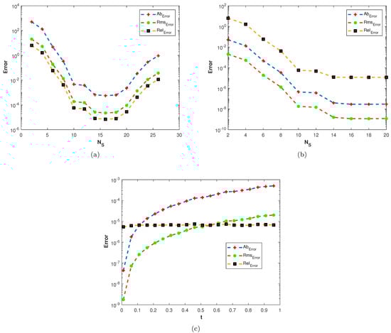
Figure 9. (a) Plots of $A{b}_{Error}$, $Rm{s}_{Error}$, and $Re{l}_{Error}$ versus $N_S$ at $T=1.$ (b) Plots of $A{b}_{Error}$, $Rm{s}_{Error}$, and $Re{l}_{Error}$ versus $N_S$ at $T=0.01.$ (c) Plots of $A{b}_{Error}$, $Rm{s}_{Error}$, and $Re{l}_{Error}$ versus t with ${\mathcal{G}}_N=625$, ${\sigma }_n=20,N_S=18$.

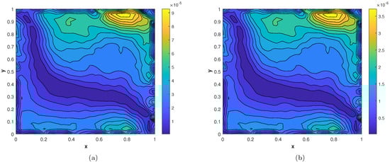
Figure 10. (a) Contour plot of $A{b}_{Error}$. (b) Contour plot of $Rm{s}_{Error}$.

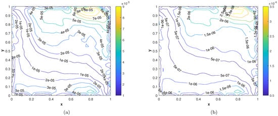
Figure 11. (a) Contour plot of $A{b}_{Error}$. (b) Contour plot of $Rm{s}_{Error}$.

4.3. Problem 3

In our third experiment, we consider a $2D$ TFDE with zero Dirichlet boundary conditions in a domain $\mathrm{\Xi }={[-1,1]}^2.$ The parameters in Equations (1)–(3) are chosen as $D=1,k=0,$ $\overrightarrow{\mathit{V}}=[0,0],$$\mathcal{Q}(\overline{\mathbf{\varsigma }},t)=0,$ $\mathcal{B}(\overline{\mathbf{\varsigma }},t)=0,$ $u_0\left(\overline{\mathbf{\varsigma }}\right)=cos\left(\frac{\pi x}{2}\right)cos\left(\frac{\pi y}{2}\right),$ $\alpha =0.90$, and the analytic solution of the problem is $u(\overline{\mathbf{\varsigma }},t)=E_{\alpha }\left(\frac{-{\pi }^2}{2}{t}^{\alpha }\right)cos\left(\frac{\pi x}{2}\right)cos\left(\frac{\pi y}{2}\right),$ in which $\overline{\mathbf{\varsigma }}=(x,y)\in \mathrm{\Xi },$ where $E_{\alpha }\left(z\right)$ is the one parameter Mittage–Liffler function defined by $E_{\alpha }\left(z\right)={\sum }_{j=0}^{\infty }\frac{z^j}{\mathrm{\Gamma }(\alpha j+1)}.$ The errors of the proposed numerical method are presented in Table 3. In this problem also, the results are obtained for various values of ${\sigma }_n,N_S,{\mathcal{G}}_N$ and $\alpha =0.90.$ Figure 12a displays the numerical solution of the problem. Figure 12b and Figure 13 show the plots of $A{b}_{Error}$, and $Rm{s}_{Error}$ errors, respectively. In Figure 14a,b, the plots show a comparison of the three error norms for various values of $N_S$ at $T=1$ and $T=0.01$, and similar behavior of the error norms is observed. In Figure 14c, a comparison between the three error norms versus t is shown. Figure 15 and Figure 16 shows the contour plots of $A{b}_{Error}$, and $Rm{s}_{Error}$. From the graphs and table, it is evident that the proposed method has solved this problem with acceptable accuracy.

Table 3. The errors obtained using the proposed scheme at final time $T=1$ for problem 3.

$\mathit{\alpha }=0.90$	${\mathit{\sigma }}_{\mathit{n}}$	$\mathit{A}{\mathit{b}}_{\mathit{E}\mathit{r}\mathit{r}\mathit{o}\mathit{r}}$	$\mathit{R}\mathit{m}{\mathit{s}}_{\mathit{E}\mathit{r}\mathit{r}\mathit{o}\mathit{r}}$	$\mathit{R}\mathit{e}{\mathit{l}}_{\mathit{E}\mathit{r}\mathit{r}\mathit{o}\mathit{r}}$	CPU(s)
	20	1.5787$\times {10}^{-4}$	6.3150$\times {10}^{-6}$	3.7390$\times {10}^{-4}$	0.887272
$(N_S,{\mathcal{G}}_N)=(18,625)$	21	1.4402$\times {10}^{-4}$	5.7610$\times {10}^{-6}$	3.4110$\times {10}^{-4}$	0.832852
	22	9.2418$\times {10}^{-5}$	3.6967$\times {10}^{-6}$	2.1888$\times {10}^{-4}$	0.870290
	23	2.8984$\times {10}^{-5}$	1.1594$\times {10}^{-6}$	6.8645$\times {10}^{-5}$	0.969934
	24	3.4135$\times {10}^{-5}$	1.3654$\times {10}^{-6}$	8.0845$\times {10}^{-5}$	0.912345
	25	3.8871$\times {10}^{-5}$	1.5548$\times {10}^{-6}$	9.2061$\times {10}^{-5}$	1.039839
	26	3.0696$\times {10}^{-5}$	1.2278$\times {10}^{-6}$	7.2699$\times {10}^{-5}$	1.000615
$\alpha =0.90$	${\mathcal{G}}_N$	$A{b}_{Error}$	$Rm{s}_{Error}$	$Re{l}_{Error}$	CPU(s)
	484	2.0243$\times {10}^{-4}$	9.2016$\times {10}^{-6}$	5.4793$\times {10}^{-4}$	0.754501
$(N_S,{\sigma }_n)=(18,25)$	529	2.8677$\times {10}^{-5}$	1.2468$\times {10}^{-6}$	7.4092$\times {10}^{-5}$	0.787635
	576	5.3314$\times {10}^{-5}$	2.2214$\times {10}^{-6}$	1.3176$\times {10}^{-4}$	0.777492
	625	3.8871$\times {10}^{-5}$	1.5548$\times {10}^{-6}$	9.2061$\times {10}^{-5}$	0.877768
	676	4.0459$\times {10}^{-5}$	1.5561$\times {10}^{-6}$	9.1988$\times {10}^{-5}$	1.037267
	729	3.4507$\times {10}^{-5}$	1.2780$\times {10}^{-6}$	7.5438$\times {10}^{-5}$	0.965576
$\alpha =0.90$	$N_S$	$A{b}_{Error}$	$Rm{s}_{Error}$	$Re{l}_{Error}$	CPU(s)
	10	2.4250$\times {10}^{-3}$	8.0833$\times {10}^{-5}$	4.7530$\times {10}^{-3}$	0.976971
$({\mathcal{G}}_N,{\sigma }_n)=(900,20)$	12	7.6536$\times {10}^{-4}$	2.5512$\times {10}^{-5}$	1.5001$\times {10}^{-4}$	1.074337
	14	4.6386$\times {10}^{-5}$	1.5462$\times {10}^{-6}$	9.0918$\times {10}^{-5}$	1.101967
	16	1.2244$\times {10}^{-4}$	4.0813$\times {10}^{-6}$	2.3998$\times {10}^{-4}$	1.095336
	18	1.0368$\times {10}^{-4}$	3.4560$\times {10}^{-6}$	2.0322$\times {10}^{-4}$	1.120181

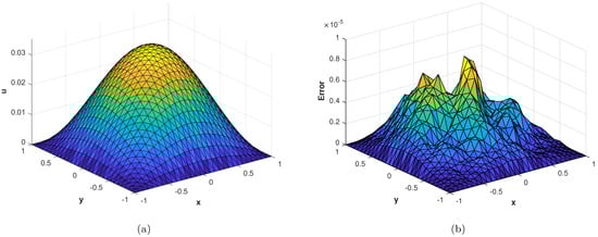
Figure 12. (a) Numerical solution of problem 3. (b) $A{b}_{Error}$ of the proposed method with ${\mathcal{G}}_N=900$, $N_S=18,{\sigma }_n=20$ at $T=1$ corresponding to problem 3.

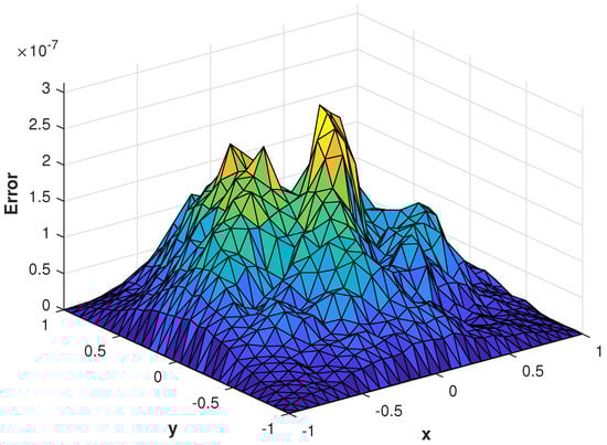
Figure 13. $Rm{s}_{Error}$ of the proposed method with ${\mathcal{G}}_N=900,N_S=18,{\sigma }_n=20$ at $T=1$ corresponding to problem 3.

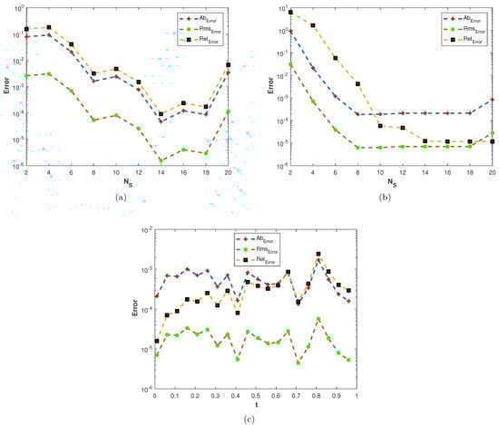
Figure 14. (a) Plots of $A{b}_{Error}$, $Rm{s}_{Error}$, and $Re{l}_{Error}$ versus $N_S$ at $T=1.$ (b) Plots of $A{b}_{Error}$, $Rm{s}_{Error}$, and $Re{l}_{Error}$ versus $N_S$ with ${\mathcal{G}}_N=900,{\sigma }_n=20$ at $T=0.01.$ (c) Plots of $A{b}_{Error}$, $Rm{s}_{Error}$, and $Re{l}_{Error}$ versus $N_S$ versus t with ${\mathcal{G}}_N=900,{\sigma }_n=20,N_S=18$.

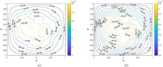
Figure 15. (a) Contour plot of $A{b}_{Error}$ at time level $T=1.$ (b) Contour plot $Rm{s}_{Error}$ at time level $T=1$.

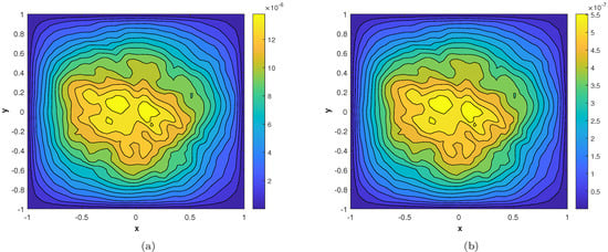
Figure 16. (a) Contour plot of $A{b}_{Error}$ at time level $T=1.$ (b) Contour plot of $Rm{s}_{Error}$ at time level $T=1$.

4.4. Problem 4

In the last experiment, we consider the $3D$ TFDE with Dirichlet boundary conditions in a domain $\mathrm{\Xi }={[0,2]}^3.$ The parameters in Equations (1)–(3) are chosen as $D=1$, $k=1,$ $\overrightarrow{\mathit{V}}=[0,0,0],$ $\mathcal{B}(\overline{\mathbf{\varsigma }},t)=t^2\left[x(2-x)+y(2-y)+z(2-z)\right],$ $\mathcal{Q}(\overline{\mathbf{\varsigma }},t)=\left[\frac{2t^{(2-\alpha )}}{\mathrm{\Gamma }(3-\alpha )}+t^2\right]$$\left[x(2-x)+y(2-y)+z(2-z)\right]+6t^2,$ $u_0\left(\overline{\mathbf{\varsigma }}\right)=0,$$\alpha =0.90$, and the analytic solution of the problem is $u(\overline{\mathbf{\varsigma }},t)=t^2\left[x(2-x)+y(2-y)+z(2-z)\right],$ in which $\overline{\mathbf{\varsigma }}=(x,y,z)\in \mathrm{\Xi }.$ Table 4 shows the accuracy of the proposed method by using different values of ${\mathcal{G}}_N,N_S,{\sigma }_n$ and $\alpha =0.90$ at final time $T=1$. The slice plots of analytic and numerical solutions are depicted in Figure 17a,b from which the accuracy of the proposed numerical scheme is evident. In Figure 18a,b, the plots show a comparison of the three error norms for various values of $N_S$ at final time $T=1$ and $T=0.01.$ Figure 18c shows a comparison between the three error norms for various values of t. Figure 19a,b shows the contour plots of $A{b}_{Error}$ and $Rm{s}_{Error}$. In Figure 20a,b, the plots of absolute error at time levels $T=0.01$ and $T=1$ are shown. The numerical solutions at the $z=1$ cross section at time instants $T=0.01$ and $T=1$ are depicted in Figure 21a,b. We can see that the method has performed very efficiently for this problem as well.

Table 4. The errors obtained using the proposed scheme at final time $T=1$ for problem 4.

$\mathit{\alpha }=0.9$	${\mathcal{G}}_{\mathit{N}}$	$\mathit{A}{\mathit{b}}_{\mathit{E}\mathit{r}\mathit{r}\mathit{o}\mathit{r}}$	$\mathit{R}\mathit{m}{\mathit{s}}_{\mathit{E}\mathit{r}\mathit{r}\mathit{o}\mathit{r}}$	$\mathit{R}\mathit{e}{\mathit{l}}_{\mathit{E}\mathit{r}\mathit{r}\mathit{o}\mathit{r}}$	CPU(s)
	729	2.4631$\times {10}^{-4}$	1.0781$\times {10}^{-4}$	5.7929$\times {10}^{-5}$	5.831264
$(N_S,{\sigma }_n)=(20,80)$	1000	1.8778$\times {10}^{-4}$	9.6171$\times {10}^{-5}$	5.1065$\times {10}^{-5}$	8.208304
	1331	3.7038$\times {10}^{-4}$	8.0097$\times {10}^{-5}$	4.2130$\times {10}^{-5}$	12.144358
	1728	1.6588$\times {10}^{-4}$	7.3857$\times {10}^{-5}$	3.8551$\times {10}^{-5}$	17.086863
	2197	2.6392$\times {10}^{-4}$	8.7479$\times {10}^{-5}$	4.5370$\times {10}^{-5}$	25.868403
$\alpha =0.9$	$N_S$	$A{b}_{Error}$	$Rm{s}_{Error}$	$Re{l}_{Error}$	CPU(s)
	16	2.0937$\times {10}^{-4}$	6.9537$\times {10}^{-5}$	3.6576$\times {10}^{-5}$	11.743146
$({\mathcal{G}}_N,{\sigma }_n)=(1331,50)$	18	2.0961$\times {10}^{-4}$	6.9627$\times {10}^{-5}$	3.6623$\times {10}^{-5}$	13.808768
	20	2.0930$\times {10}^{-4}$	7.0879$\times {10}^{-5}$	3.7282$\times {10}^{-5}$	11.128933
	22	3.0057$\times {10}^{-4}$	8.5166$\times {10}^{-5}$	4.4797$\times {10}^{-5}$	11.274943
$\alpha =0.9$	${\sigma }_n$	$A{b}_{Error}$	$Rm{s}_{Error}$	$Re{l}_{Error}$	CPU(s)
	71	2.0501$\times {10}^{-4}$	8.2774$\times {10}^{-5}$	4.3539$\times {10}^{-5}$	14.044730
$({\mathcal{G}}_N,N_S)=(1331,18)$	72	2.0674$\times {10}^{-4}$	8.0409$\times {10}^{-5}$	4.2295$\times {10}^{-5}$	14.006118
	73	2.5473$\times {10}^{-4}$	8.2782$\times {10}^{-5}$	4.3543$\times {10}^{-5}$	16.449350
	74	2.0207$\times {10}^{-4}$	8.2277$\times {10}^{-5}$	4.3277$\times {10}^{-5}$	16.104030

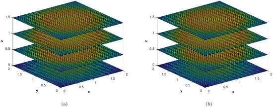
Figure 17. (a) Slice plot of analytic solution corresponding to problem 4. (b) Slice plot of numerical solution corresponding to problem 4.

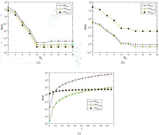
Figure 18. (a) Plots of Plots of $A{b}_{Error}$, $Rm{s}_{Error}$, and $Re{l}_{Error}$ versus $N_S$ with ${\mathcal{G}}_N=4913,{\sigma }_n=80$ at $T=1.$ (b) Plots of Plots of $A{b}_{Error}$, $Rm{s}_{Error}$, and $Re{l}_{Error}$ versus $N_S$ with ${\mathcal{G}}_N=4096,{\sigma }_n=80$ at $T=0.01.$ (c) Plots of Plots of $A{b}_{Error}$, $Rm{s}_{Error}$, and $Re{l}_{Error}$ versus t with ${\mathcal{G}}_N=4913,{\sigma }_n=80$, alpha = 0.9, $N_S=18$.

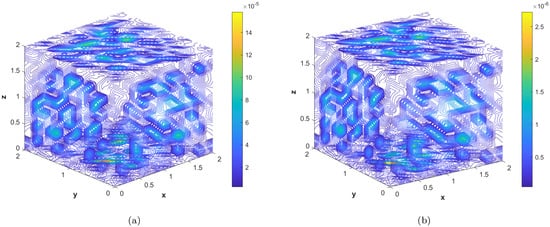
Figure 19. (a) Contour plot of $A{b}_{Error}$ at time level $T=1$. (b) Contour plot of $Rm{s}_{Error}$ with ${\mathcal{G}}_N=3375,{\sigma }_n=80,N_S=20$ at time level $T=1$.

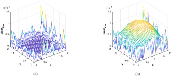
Figure 20. (a) Plot of $A{b}_{Error}$ with ${\mathcal{G}}_N=900,N_S=18,{\sigma }_n=30,\alpha =0.9,z=1$ at $T=0.01$. (b) Plot of $A{b}_{Error}$ with ${\mathcal{G}}_N=900,N_S=18,{\sigma }_n=30,\alpha =0.9,z=1$ at $T=1$.

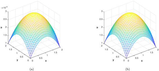
Figure 21. (a) The numerical solution at $z=1$ cross section with ${\mathcal{G}}_N=900,N_S=18,{\sigma }_n=30,\alpha =0.9$ at $T=0.01$. (b) The numerical solution at $z=1$ cross section with ${\mathcal{G}}_N=900,N_S=18,{\sigma }_n=30$, $\alpha =0.9$ at $T=1$.

5. Conclusions

This article develops a numerical method based on LT- and RBF-based local meshless methods for approximating the solution of multi-dimensional diffusion problems of fractional order. In contrast to the standard FDM for temporal discretization, the proposed scheme implements Laplace transform and Stehfest’s method to handle the time-fractional derivative. The RBF-based local meshless is used to avoid the ill-conditioning of interpolation matrices. The RBF-based local meshless method is based on local interpolation matrices and works well when a large number of nodes is used. This method has low computational cost since many small-size matrices are inverted only once outside the time-loop instead of a large matrix. The convergence and stability of the method are discussed. Problems in one, two and three dimensions are solved. The obtained results were compared with other methods, and it is observed that the proposed method has produced better results. From the error analysis and computational results presented in the tables and figures, one can observe that the proposed method is an efficient and competitive method for the solution of fractional diffusion problems.

References

- Podlubny, I. Fractional Differential Equations; Academic Press: San Diego, CA, USA, 1999. [Google Scholar]
- Miller, K.S.; Ross, B. An Introduction to the Fractional Calculus and Fractional Differential Equations; Wiley: Hoboken, NJ, USA, 1993. [Google Scholar]
- Samko, S.G.; Kilbas, A.A.; Marichev, O.I. Fractional Integrals and Derivatives (Theory and Applications); Gordon and Breach Science Publishers: Basel, Switzerland, 1993. [Google Scholar]
- Metzler, R.; Klafter, J. The random walk’s guide to anomalous diffusion: A fractional dynamics approach. Phys. Rep. 2000, 339, 1–77. [Google Scholar] [CrossRef]
- Hilfer, R. (Ed.) Applications of Fractional Calculus in Physics; World Scientific: Singapore, 2000. [Google Scholar]
- Gorenflo, R.; Mainardi, F.; Moretti, D.; Pagnini, G.; Paradisi, P. Discrete random walk models for space–time fractional diffusion. Chem. Phys. 2002, 284, 521–541. [Google Scholar] [CrossRef]
- Scher, H.; Montroll, E.W. Anomalous transit–time dispersion in amorphous solids. Phys. Rev. B 1975, 12, 2455. [Google Scholar] [CrossRef]
- Hristov, J. Magnetic field diffusion in ferromagnetic materials: Fractional calculus approaches. Int. J. Optim. Control. Theor. Appl. (IJOCTA) 2021, 11, 1–15. [Google Scholar] [CrossRef]
- Macías-Díaz, J.E. On a discrete model that dissipates the free energy of a time-space fractional generalized nonlinear parabolic equation. Appl. Numer. Math. 2022, 172, 215–223. [Google Scholar] [CrossRef]
- Shao, X.H.; Kang, C.B. A preconditioner based on sine transform for space fractional diffusion equations. Appl. Numer. Math. 2022, 178, 248–261. [Google Scholar] [CrossRef]
- Witten, T.A. Insights from soft condensed matter. Rev. Mod. Phys. 1999, 71, 367–373. [Google Scholar] [CrossRef]
- Chang, F.X.; Chen, J.; Huang, W. Anomalous diffusion and fractional advection-diffusion equation. Acta Phys. Sin. 2005, 54, 1113–1117. [Google Scholar] [CrossRef]
- Wyss, W. The fractional diffusion equation. J. Math. Phys. 1986, 27, 2782–2785. [Google Scholar] [CrossRef]
- Meerschaert, M.M.; Tadjeran, C. Finite difference approximations for fractional advection-dispersion flow equations. J. Comput. Appl. Math. 2004, 172, 65–77. [Google Scholar] [CrossRef]
- Greenenko, A.A.; Chechkin, A.V.; Shul’ga, N.F. Anomalous diffusion and Lévy flights in channeling. Phys. Lett. A 2004, 324, 82–85. [Google Scholar] [CrossRef]
- Chen, W. Time-space fabric underlying anomalous diffusion. Chaos Solitons Fractals 2006, 28, 923–929. [Google Scholar] [CrossRef]
- Chen, W.; Sun, H.; Zhang, X.; Korošak, D. Anomalous diffusion modeling by fractal and fractional derivatives. Comput. Math. Appl. 2010, 59, 1754–1758. [Google Scholar] [CrossRef]
- Agrawal, O.P. Solution for a fractional diffusion-wave equation defined in a bounded domain. Nonlinear Dyn. 2002, 29, 145–155. [Google Scholar] [CrossRef]
- Bayrak, M.A.; Demir, A.; Ozbilge, E. Numerical solution of fractional diffusion equation by Chebyshev collocation method and residual power series method. Alex. Eng. J. 2020, 59, 4709–4717. [Google Scholar] [CrossRef]
- Sousa, E. Numerical approximations for fractional diffusion equations via splines. Comput. Math. Appl. 2011, 62, 938–944. [Google Scholar] [CrossRef]
- Li, C.; Zhao, Z.; Chen, Y. Numerical approximation of nonlinear fractional differential equations with subdiffusion and superdiffusion. Comput. Math. Appl. 2011, 62, 855–875. [Google Scholar] [CrossRef]
- Zheng, X.; Wang, H. Analysis and numerical approximation to time-fractional diffusion equation with a general time-dependent variable order. Nonlinear Dyn. 2021, 104, 4203–4219. [Google Scholar] [CrossRef]
- Bouchama, K.; Arioua, Y.; Merzougui, A. The numerical solution of the space-time fractional diffusion equation involving the Caputo-Katugampola fractional derivative. Numer. Algebra Control Optim. 2022, 12, 621. [Google Scholar] [CrossRef]
- Tadjeran, C.; Meerschaert, M.M.; Scheffler, H.P. A second-order accurate numerical approximation for the fractional diffusion equation. J. Comput. Phys. 2006, 213, 205–213. [Google Scholar] [CrossRef]
- Liu, F.; Anh, V.; Turner, I.; Zhuang, P. Time fractional advection dispersion equation. J. Appl. Math. Comput. 2003, 13, 233–245. [Google Scholar] [CrossRef]
- Lin, Y.; Xu, C. Finite difference/spectral approximations for the time-fractional diffusion equation. J. Comput. Phys. 2005, 225, 1533–1552. [Google Scholar] [CrossRef]
- Assari, P.; Dehghan, M. Application of dual-Chebyshev wavelets for the numerical solution of boundary integral equations with logarithmic singular kernels. Eng. Comput. 2019, 35, 175–190. [Google Scholar] [CrossRef]
- Assari, P.; Adibi, H.; Dehghan, M. A Meshless Discrete Galerkin (mdg) Method for the Numerical Solution of Integral Equations with Logarithmic Kernels. J. Comput. Appl. Math. 2014, 267, 160–181. [Google Scholar] [CrossRef]
- Dehghan, M.; Salehi, R. A meshless local Petrov-Galerkin method for the time-dependent Maxwell equations. J. Comput. Appl. Math. 2014, 268, 93–110. [Google Scholar] [CrossRef]
- Dehghan, M.; Salehi, R. The numerical solution of the non-linear integro-differential equations based on the meshless method. J. Comput. Appl. Math. 2012, 236, 2367–2377. [Google Scholar] [CrossRef]
- Sarra, S.A.; Kansa, E.J. Multiquadric radial basis function approximation methods for the numerical solution of partial differential equations. Adv. Comput. Mech. 2009, 2, 220. [Google Scholar]
- Lee, C.K.; Liu, X.; Fan, S.C. Local multiquadric approximation for solving boundary value problems. Comput. Mech. 2003, 30, 396–409. [Google Scholar] [CrossRef]
- Jackson, S.J.; Stevens, D.; Giddings, D.; Power, H. An adaptive RBF finite collocation approach to track transport processes across moving fronts. Comput. Math. Appl. 2016, 71, 278–300. [Google Scholar] [CrossRef]
- Naffa, M.; Al-Gahtani, H.J. RBF-based meshless method for large deflection of thin plates. Eng. Anal. Bound. Elem. 2007, 31, 311–317. [Google Scholar] [CrossRef]
- Leitao, V.M.A. RBF-based meshless methods for 2D elastostatic problems. Eng. Anal. Bound. Elem. 2004, 28, 1271–1281. [Google Scholar] [CrossRef]
- Dehghan, M.; Shirzadi, M. Meshless simulation of stochastic advection-diffusion equations based on radial basis functions. Eng. Anal. Bound. Elem. 2015, 53, 18–26. [Google Scholar] [CrossRef]
- Šarler, B.; Vertnik, R. Meshfree explicit local radial basis function collocation method for diffusion problems. Comput. Math. Appl. 2006, 51, 1269–1282. [Google Scholar] [CrossRef]
- Dehghan, M.; Abbaszadeh, M. Numerical investigation based on direct meshless local Petrov Galerkin (direct MLPG) method for solving generalized Zakharov system in one and two dimensions and generalized Gross-Pitaevskii equation. Eng. Comput. 2017, 33, 983–996. [Google Scholar] [CrossRef]
- Vertnik, R.; Šarler, B. Meshless local radial basis function collocation method for convective-diffusive solid-liquid phase change problems. Int. J. Numer. Methods Heat Fluid Flow 2006, 16, 617–640. [Google Scholar] [CrossRef]
- Jiwari, R.; Singh, S.; Singh, P. Local RBF-FD-Based Mesh-free Scheme for Singularly Perturbed Convection-Diffusion-Reaction Models with Variable Coefficients. J. Math. 2022, 2022, 3119482. [Google Scholar] [CrossRef]
- Kosec, G.; Šarler, B. Local RBF collocation method for Darcy flow. Comput. Model. Eng. Sci. 2008, 25, 197. [Google Scholar]
- Yao, G.; Islam, S.; Šarler, B. Assessment of global and local meshless methods based on collocation with radial basis functions for parabolic partial differential equations in three dimensions. Eng. Anal. Bound. Elem. 2012, 36, 1640–1648. [Google Scholar] [CrossRef]
- Kamran; Khan, S.; Alhazmi, S.E.; Alotaibi, F.M.; Ferrara, M.; Ahmadian, A. On the Numerical Approximation of Mobile-Immobile Advection-Dispersion Model of Fractional Order Arising from Solute Transport in Porous Media. Fractal Fract. 2022, 6, 445. [Google Scholar] [CrossRef]
- Davies, A.J.; Crann, D.; Kane, S.J.; Lai, C.H. A hybrid Laplace transform/finite difference boundary element method for diffusion problems. Comput. Model. Eng. Sci. 2007, 18, 79–86. [Google Scholar]
- Rizzo, F.J.; Shippy, D.J. A method of solution for certain problems of transient heat conduction. AIAA J. 1970, 8, 2004–2009. [Google Scholar] [CrossRef]
- Dubner, H.; Abate, J. Numerical inversion of Laplace transforms by relating them to the finite Fourier cosine transform. J. ACM (JACM) 1968, 15, 115–123. [Google Scholar] [CrossRef]
- Durbin, F. Numerical inversion of Laplace transforms: An efficient improvement to Dubner and Abate’s method. Comput. J. 1974, 17, 371–376. [Google Scholar] [CrossRef]
- Crump, K.S. Numerical inversion of Laplace transforms using a Fourier series approximation. J. ACM (JACM) 1976, 23, 89–96. [Google Scholar] [CrossRef]
- De Hoog, F.R.; Knight, J.H.; Stokes, A.N. An improved method for numerical inversion of Laplace transforms. SIAM J. Sci. Stat. Comput. 1982, 3, 357–366. [Google Scholar] [CrossRef]
- Weeks, W.T. Numerical inversion of Laplace transforms using Laguerre functions. J. ACM (JACM) 1966, 13, 419–429. [Google Scholar] [CrossRef]
- Talbot, A. The accurate numerical inversion of Laplace transforms. IMA J. Appl. Math. 1979, 23, 97–120. [Google Scholar] [CrossRef]
- Dingfelder, B.; Weideman, J.A.C. An improved Talbot method for numerical Laplace transform inversion. Numer. Algorithms 2015, 68, 167–183. [Google Scholar] [CrossRef]
- Thomée, V. A high order parallel method for time discretization of parabolic type equations based on Laplace transformation and quadrature. Int. J. Numer. Anal. Anal. Model. 2005, 2, 85–96. [Google Scholar]
- Lpez-Fernández, M.; Palencia, C. On the numerical inversion of the Laplace transform of certain holomorphic mappings. Appl. Numer. Math. 2004, 51, 289–303. [Google Scholar] [CrossRef]
- Kamran; Kamal, R.; Rahmat, G.; Shah, K. On the Numerical Approximation of Three-Dimensional Time Fractional Convection-Diffusion Equations. Math. Probl. Eng. 2021, 2021, 4640467. [Google Scholar] [CrossRef]
- Kamal, R.; Kamran; Rahmat, G.; Ahmadian, A.; Arshad, N.I.; Salahshour, S. Approximation of linear one dimensional partial differential equations including fractional derivative with non-singular kernel. Adv. Differ. Equ. 2021, 2021, 317. [Google Scholar] [CrossRef]
- Stehfest, H. Algorithm 368: Numerical inversion of Laplace transforms [D5]. Commun. ACM 1970, 13, 47–49. [Google Scholar] [CrossRef]
- Stehfest, H. Remark on algorithm 368: Numerical inversion of Laplace transforms. Commun. ACM 1970, 13, 624. [Google Scholar] [CrossRef]
- Davies, B.; Martin, B. Numerical inversion of the Laplace transform: A survey and comparison of methods. J. Comput. Phys. 1979, 33, 1–32. [Google Scholar] [CrossRef]
- Schaback, R. Error estimates and condition numbers for radial basis function interpolation. Adv. Comput. Math. 1995, 3, 251–264. [Google Scholar] [CrossRef]
- Trefethen, L.N.; Bau, I.I.I.D. Numerical Linear Algebra; Siam: Philadelphia, PA, USA, 1997; Volume 50. [Google Scholar]
- Kuznetsov, A. On the Convergence of the Gaver–Stehfest Algorithm. SIAM J. Numer. Anal. 2013, 51, 2984–2998. [Google Scholar] [CrossRef]
- Abate, J.; Valkó, P.P. Multi-precision Laplace transform inversion. Int. J. Numer. Methods Eng. 2004, 60, 979–993. [Google Scholar] [CrossRef]
- Abate, J.; Whitt, W. A unified framework for numerically inverting Laplace transforms. Informs J. Comput. 2006, 18, 408–421. [Google Scholar] [CrossRef]
- Fu, Z.J.; Chen, W.; Yang, H.T. Boundary particle method for Laplace transformed time fractional diffusion equations. J. Comput. Phys. 2013, 235, 52–66. [Google Scholar] [CrossRef]
- Chen, W.; Ye, L.; Sun, H. Fractional diffusion equations by the Kansa method. Comput. Math. Appl. 2010, 59, 1614–1620. [Google Scholar] [CrossRef]
- Liu, Q.X.; Gu, Y.; Zhuang, P.; Liu, F.; Nie, Y. An implicit RBF meshless approach for time fractional diffusion equations. Comput. Mech. 2011, 48, 1–12. [Google Scholar] [CrossRef]
Disclaimer/Publisher’s Note: The statements, opinions and data contained in all publications are solely those of the individual author(s) and contributor(s) and not of MDPI and/or the editor(s). MDPI and/or the editor(s) disclaim responsibility for any injury to people or property resulting from any ideas, methods, instructions or products referred to in the content. |
© 2023 by the authors. Licensee MDPI, Basel, Switzerland. This article is an open access article distributed under the terms and conditions of the Creative Commons Attribution (CC BY) license (https://creativecommons.org/licenses/by/4.0/).