Conservative Continuous-Stage Stochastic Runge–Kutta Methods for Stochastic Differential Equations

Abstract

In this paper, we develop a new class of conservative continuous-stage stochastic Runge–Kutta methods for solving stochastic differential equations with a conserved quantity. The order conditions of the continuous-stage stochastic Runge–Kutta methods are given based on the theory of stochastic B-series and multicolored rooted tree. Sufficient conditions for the continuous-stage stochastic Runge–Kutta methods preserving the conserved quantity of stochastic differential equations are derived in terms of the coefficients. Conservative continuous-stage stochastic Runge–Kutta methods of mean square convergence order 1 for general stochastic differential equations, as well as conservative continuous-stage stochastic Runge–Kutta methods of high order for single integrand stochastic differential equations, are constructed. Numerical experiments are performed to verify the conservative property and the accuracy of the proposed methods in the longtime simulation.

1. Introduction

Stochastic differential equations (SDEs) are widely used to model stochastic phenomena in physics, engineering, finance, biology, etc. [1]. Since analytical solutions are not available for most SDEs, numerical methods for solving SDEs have been flourishing in recent years [2].

Since many systems have important geometrical or physical properties, such as symplectic structure and conserved quantity, it is quite natural to look forward to numerical methods that can preserve the peculiarities of the original systems. Such methods are usually called structure-preserving numerical methods. Extensive numerical experiments have exhibited the distinct advantage of structure-preserving numerical methods, especially in longtime numerical simulations. It is well known that the theory of conserved quantities or first integrals is a very significant subject for dynamical systems, because such quantities usually represent fundamental characteristics of these systems. Therefore, research on the numerical methods preserving the conserved quantities of dynamical systems is very important when it comes to performing reliable numerical simulations. Fruitful numerical methods preserving single or multiple conserved quantities for ordinary differential equations (ODEs) have been derived over the past few decades (e.g., [3,4,5,6,7,8,9,10,11,12,13,14,15,16,17,18,19]). Nevertheless, such conservative numerical methods for SDEs are less developed. As far as we know, the existing conservative numerical methods for SDEs mainly consist of difference methods [20], discrete gradient methods [21,22,23], projection methods [22,24], averaged vector field methods [25,26], and a few others.

As is well known, Runge–Kutta methods are not conservative in general; however, continuous-stage Runge–Kutta (CSRK) methods can overcome the difficulties. CSRK methods were first presented by Butcher in the 1970s [27], and are considered an extension of traditional Runge–Kutta methods. For ODEs, CSRK methods have been investigated recently in the construction of energy-preserving methods [4,6,9,16,17]. It is worth mentioning that many existing energy-preserving methods for ODEs, such as average vector field methods [10], energy-preserving trapezoidal methods [11], Hamiltonian boundary value methods [12,13], continuous time finite element methods [14,15], and energy-preserving collocation methods [6] all lie in the framework of CSRK methods. Ref. [8] studies the sufficient energy-preserving conditions of CSRK methods for solving Hamiltonian systems. Motivated by which, and in view of the fact that there has been little research on CSRK methods for SDEs so far, in this work, we aim to develop the conservative continuous-stage stochastic Runge–Kutta (CSSRK) methods to solve SDEs with a general conserved quantity.

The rest of the paper is organized as follows. In Section 2, we present the CSSRK methods for general SDEs. On the basis of the stochastic B-series theory, we obtain the order conditions. In Section 3, we apply the CSSRK methods to SDEs with a conserved quantity to derive the conservative conditions. Furthermore, we derive the conservative conditions in terms of the coefficients of the polynomials. In Section 4, we construct conservative CSSRK methods of mean square convergence order 1 for general conservative SDEs and conservative CSSRK methods of high order for single integrand conservative SDEs. Numerical experiments are conducted to verify the theoretical results in Section 5. Some conclusions and remarks on our work are given in Section 6.

2. CSSRK Methods and Order Conditions

Consider the stochastic differential equation (SDE) with d noises in the Stratonovich sense

$$\left\{\begin{array}{c}dX\left(t\right)=g_0\left(X\left(t\right)\right)dt+{\displaystyle \sum _{k=1}^d}{g}_k\left(X\left(t\right)\right)\circ d{W}_k\left(t\right),t\in [0,T],\hfill \\ X\left(0\right)=x_0\in {\mathbb{R}}^M,\hfill \end{array}\right.$$

(1)

where $W_k\left(t\right)(k=1,\dots ,d)$ are pairwise independent one-dimensional Wiener processes, defined on a complete filtered probability space ($\Omega ,\mathcal{F},\mathbb{P},{\left\{\mathcal{F}\right\}}_{t⩾0}$) fulfilling the usual conditions. We assume the initial value vector $x_0$ is ${\mathcal{F}}_0$-measurable with $E\parallel x_0{\parallel }^2<\infty$; the vector fields $g_k:{\mathbb{R}}^M\to {\mathbb{R}}^M$, $k=0,1,\dots ,d$, are sufficiently smooth and satisfy certain conditions, such that (1) has a unique solution.

For a uniform partition of the interval $[0,T]$, $0=t_0<t_1<\cdots <t_N=T$, let $y_n$ denote the numerical approximation of $X\left(t\right)$ at $t_n=nh,n=0,1,\dots ,N$. Given $y_0=x_0$, we define the following one-step method as the CSSRK method for solving (1)

$$\begin{array}{c}{Y}_{\tau }=y_0+h{\int }_0^1{A}_{\tau ,\xi }{g}_0\left(Y_{\xi }\right)d\xi +{\displaystyle \sum _{k=1}^d}{\displaystyle \sum _{r=1}^{\overline{r}}}{\omega }_{r,k}{\int }_0^1{\tilde{A}}_{\tau ,\xi }^{r,k}{g}_k\left(Y_{\xi }\right)d\xi ,\hfill \\ y_1=y_0+h{\int }_0^1{B}_{\xi }{g}_0\left(Y_{\xi }\right)d\xi +{\displaystyle \sum _{k=1}^d}{\displaystyle \sum _{r=1}^{\overline{r}}}{\omega }_{r,k}{\int }_0^1{\tilde{B}}_{\xi }^{r,k}{g}_k\left(Y_{\xi }\right)d\xi ,\hfill \end{array}$$

(2)

where ${\omega }_{r,k}$ are a series of random variables, $A_{\tau ,\xi }$ and ${\tilde{A}}_{\tau ,\xi }^{r,k}$ are bivariate polynomials with respect to $\tau$, and $\xi$, $B_{\xi }$ and ${\tilde{B}}_{\xi }^{r,k}$ are polynomials with respect to $\xi$, $k=1,\dots ,d,r=1,\dots ,\overline{r}$. There is a restrictive relation between the internal and final stages for the consistency of the method, because $y_1$ should coincide with $Y_1$ [8]. Therefore, $B_{\xi }$ is equal to $A_{1,\xi }$ and ${\tilde{B}}_{\xi }^{r,k}$ is equal to ${\tilde{A}}_{1,\xi }^{r,k}$.

If we denote $h{A}_{\tau ,\xi }=Z_{\tau ,\xi }^{\left(0\right)}$, ${\displaystyle \sum _{r=1}^{\overline{r}}}{\omega }_{r,k}{\tilde{A}}_{\tau ,\xi }^{r,k}=Z_{\tau ,\xi }^{\left(k\right)}$, $h{B}_{\xi }=z_{\xi }^{\left(0\right)}$, ${\displaystyle \sum _{r=1}^{\overline{r}}}{\omega }_{r,k}{\tilde{B}}_{\xi }^{r,k}=z_{\xi }^{\left(k\right)}$, then a more brief representation of (2) is derived as

$$\begin{array}{c}{Y}_{\tau }=y_0+{\displaystyle \sum _{k=0}^d}{\int }_0^1{Z}_{\tau ,\xi }^{\left(k\right)}{g}_k\left(Y_{\xi }\right)d\xi ,\hfill \\ y_1=y_0+{\displaystyle \sum _{k=0}^d}{\int }_0^1{z}_{\xi }^{\left(k\right)}{g}_k\left(Y_{\xi }\right)d\xi .\hfill \end{array}$$

(3)

Next, we show the order conditions of the CSSRK method (2). First, we recall some definitions and lemmas about stochastic B-series and multicolored rooted trees, which are very important tools used to perform local error analysis. The B-series theory for ODEs was introduced by Butcher in 1963 [28], and B-series for SDEs was developed in the past few decades (e.g., [29,30,31,32]).

Definition 1.

([30] Trees). The set of multicolored rooted trees

$$T=\{\varnothing \}\cup T_0\cup T_1\cup \cdots \cup T_d$$

is recursively defined by

 (I)

The graph ${•}_k={[\varnothing ]}_k$ with only one vertex of color k belongs to $T_k$.

 (II)

If ${\tau }_1,{\tau }_2,\dots ,{\tau }_l\in T$, then $t={[{\tau }_1,{\tau }_2,\dots ,{\tau }_l]}_k\in T_k$, where $t={[{\tau }_1,{\tau }_2,\dots ,{\tau }_l]}_k$ denotes the tree formed by joining the subtrees ${\tau }_1,{\tau }_2,\dots ,{\tau }_l$, each by a single branch to a common root of color k.

Thus, $T_k$ is the set of trees with a k-colored root, and T is the union of these sets.

Definition 2.

([30] Elementary differentials). For a tree $t\in T$, the elementary differential is a mapping $F\left(t\right):{\mathbb{R}}^M\to {\mathbb{R}}^M$ defined recursively by

 (I)

$F(\varnothing )\left(x_0\right)=x_0$.

 (II)

$F\left({•}_k\right)\left(x_0\right)=g_k\left(x_0\right)$.

 (III)

If $t={[{\tau }_1,{\tau }_2,\dots ,{\tau }_l]}_k\in T_k$, then

$$F\left(t\right)\left(x_0\right)=g_k^{\left(l\right)}\left(x_0\right)(F\left({\tau }_1\right)\left(x_0\right),F\left({\tau }_2\right)\left(x_0\right),\dots ,F\left({\tau }_l\right)\left(x_0\right)).$$

A stochastic B-series is a formal series of the form

$$B(\phi ,x_0;h)=\sum _{t\in T}\alpha \left(t\right)·\phi \left(t\right)\left(h\right)·F\left(t\right)\left(x_0\right),$$

where $\alpha \left(t\right)$ is defined by

$$\alpha (\varnothing )=1,\alpha \left({•}_k\right)=1,\alpha \left({[{\tau }_1,\dots ,{\tau }_l]}_k\right)=\frac{1}{{\mu }_1!{\mu }_2!\cdots }\prod _{j=1}^l\alpha \left({\tau }_j\right),$$

where ${\mu }_1,{\mu }_2,\dots$ count equal trees among ${\tau }_1,\dots ,{\tau }_l$.

The next lemma shows that if $Y\left(h\right)$ is a B-series, then $g_k\left(Y\left(h\right)\right)$ can be written as a similar series, which is essential to derive a B-series of the exact solution and the numerical solution.

Lemma 1.

([30]). If $Y\left(h\right)$ is a B-series $B(\phi ,x_0;h)$ as

$$Y\left(h\right)=B(\phi ,x_0;h)=\sum _{t\in T}\alpha \left(t\right)·\phi \left(t\right)\left(h\right)·F\left(t\right)\left(x_0\right),$$

then $g_k\left(Y\left(h\right)\right)$ can be represented as a formal series

$$g_k\left(Y\left(h\right)\right)=\sum _{t\in T_k}\alpha \left(t\right)·{\phi }_k^{\prime }\left(t\right)\left(h\right)·F\left(t\right)\left(x_0\right),$$

for $k=0,\dots ,d$, where

$${\phi }_k^{\prime }\left(t\right)\left(h\right)=\left\{\begin{array}{cc}1,\hfill & ift={•}_k,\hfill \\ {\displaystyle \prod _{j=1}^l}\phi \left({\tau }_j\right)\left(h\right),\hfill & ift={[{\tau }_1,\dots ,{\tau }_l]}_k\in T_k.\hfill \end{array}\right.$$

Lemma 2.

([30]). The exact solution $X(t_0+h)$ of (1) can be written as a B-series $B(\varphi ,x_0;h)$

$$X(t_0+h)=B(\varphi ,x_0;h)=\sum _{t\in T}\alpha \left(t\right)·\varphi \left(t\right)\left(h\right)·F\left(t\right)\left(x_0\right),$$

with

$$\begin{array}{c}\varphi (\varnothing )\left(h\right)=1,\varphi \left({•}_k\right)\left(h\right)=W_k\left(h\right),\hfill \\ \varphi \left({[{\tau }_1,\dots ,{\tau }_l]}_k\right)\left(h\right)={\int }_0^h{\displaystyle \prod _{j=1}^l}\varphi \left({\tau }_j\right)\left(s\right)\ast d{W}_k\left(s\right),\hfill \end{array}$$

for all ${[{\tau }_1,\dots ,{\tau }_l]}_k\in T_k,k=0,1,\dots ,d$, where $W_0\left(h\right)=h$, $\ast d{W}_0\left(s\right)=ds$ and $\ast d{W}_k\left(s\right)=\circ d{W}_k\left(s\right)$ for $k=1,\dots ,d$.

In the following theorem, we prove the numerical solution using the CSSRK method (3) can be represented in the form of a B-series.

Theorem 1.

The continuous-stage values $Y_{\tau }$ and the numerical solution $Y_1$ in the CSSRK method (3) can be written in the form of B-series

$$\begin{array}{c}{Y}_{\tau }=B({\Psi }_{\tau },y_0;h)={\displaystyle \sum _{t\in T}}\alpha \left(t\right)·{\Psi }_{\tau }\left(t\right)\left(h\right)·F\left(t\right)\left(y_0\right),\hfill \\ Y_1=B(\Phi ,y_0;h)={\displaystyle \sum _{t\in T}}\alpha \left(t\right)·\Phi \left(t\right)\left(h\right)·F\left(t\right)\left(y_0\right),\hfill \end{array}$$

with

$$\begin{array}{c}{\Psi }_{\tau }(\varnothing )\left(h\right)=1,{\Psi }_{\tau }\left({•}_k\right)\left(h\right)={\int }_0^1{Z}_{\tau ,\xi }^{\left(k\right)}d\xi ,\hfill \\ {\Psi }_{\tau }\left({[{\tau }_1,\dots ,{\tau }_l]}_k\right)\left(h\right)={\int }_0^1{Z}_{\tau ,\xi }^{\left(k\right)}{\displaystyle \prod _{j=1}^l}{\Psi }_{\xi }\left({\tau }_j\right)\left(h\right)d\xi ,\hfill \end{array}$$

(4)

and

$$\begin{array}{c}\Phi (\varnothing )\left(h\right)=1,\Phi \left({•}_k\right)\left(h\right)={\int }_0^1{z}_{\xi }^{\left(k\right)}d\xi ,\hfill \\ \Phi \left({[{\tau }_1,\dots ,{\tau }_l]}_k\right)\left(h\right)={\int }_0^1{z}_{\xi }^{\left(k\right)}{\displaystyle \prod _{j=1}^l}{\Psi }_{\xi }\left({\tau }_j\right)\left(h\right)d\xi ,\hfill \end{array}$$

(5)

for all ${[{\tau }_1,\dots ,{\tau }_l]}_k\in T_k,k=0,1,\dots ,d$.

Proof. 

Following the way in [30], we write $Y_{\tau }$ as a B-series

$$Y_{\tau }=\sum _{t\in T}\alpha \left(t\right)·{\Psi }_{\tau }\left(t\right)\left(h\right)·F\left(t\right)\left(y_0\right).$$

(6)

By use of Lemma 1 together with the first equality of (3), we get

$$\begin{array}{cc}{Y}_{\tau }\hfill & =y_0+{\displaystyle \sum _{k=0}^d}{\int }_0^1{Z}_{\tau ,\xi }^{\left(k\right)}{\displaystyle \sum _{t\in T_k}}\alpha \left(t\right)·{\Psi }_{\xi ,k}^{\prime }\left(t\right)\left(h\right)·F\left(t\right)\left(y_0\right)d\xi \hfill \\ \hfill & =y_0+{\displaystyle \sum _{k=0}^d}{\displaystyle \sum _{t\in T_k}}\alpha \left(t\right)·{\int }_0^1{Z}_{\tau ,\xi }^{\left(k\right)}{\Psi }_{\xi ,k}^{\prime }\left(t\right)\left(h\right)d\xi ·F\left(t\right)\left(y_0\right),\hfill \end{array}$$

(7)

where

$${\Psi }_{\xi ,k}^{\prime }\left(t\right)\left(h\right)=\left\{\begin{array}{c}1,ift={•}_k,\hfill \\ {\displaystyle \prod _{j=1}^l}{\Psi }_{\xi }\left({\tau }_j\right)\left(h\right),ift={[{\tau }_1,\dots ,{\tau }_l]}_k\in T_k.\hfill \end{array}\right.$$

(8)

Comparing (6) with (7) term by term, we obtain (4).

Similarly, we write

$$Y_1=\sum _{t\in T}\alpha \left(t\right)·\Phi \left(t\right)\left(h\right)·F\left(t\right)\left(y_0\right).$$

(9)

By means of the second equality of (3), Lemma 1 and (6), we obtain

$$\begin{array}{cc}{Y}_1\hfill & =y_0+{\displaystyle \sum _{k=0}^d}{\int }_0^1{z}_{\xi }^{\left(k\right)}{\displaystyle \sum _{t\in T_k}}\alpha \left(t\right)·{\Psi }_{\xi ,k}^{\prime }\left(t\right)\left(h\right)·F\left(t\right)\left(y_0\right)d\xi \hfill \\ \hfill & =y_0+{\displaystyle \sum _{k=0}^d}{\displaystyle \sum _{t\in T_k}}\alpha \left(t\right)·{\int }_0^1{z}_{\xi }^{\left(k\right)}{\Psi }_{\xi ,k}^{\prime }\left(t\right)\left(h\right)d\xi ·F\left(t\right)\left(y_0\right),\hfill \end{array}$$

(10)

where

$${\Psi }_{\xi ,k}^{\prime }\left(t\right)\left(h\right)=\left\{\begin{array}{c}1,ift={•}_k,\hfill \\ {\displaystyle \prod _{j=1}^l}{\Psi }_{\xi }\left({\tau }_j\right)\left(h\right),ift={[{\tau }_1,\dots ,{\tau }_l]}_k\in T_k,\hfill \end{array}\right.$$

(11)

then, comparing (9) with (10) term by term gives (5). □

Definition 3.

([30]). The order of a tree $t\in T$ is defined by

$$\rho (\varnothing )=0,\rho (t={[{\tau }_1,\dots ,{\tau }_l]}_k)={\displaystyle \sum _{j=1}^l}\rho \left({\tau }_j\right)+\left\{\begin{array}{c}1,fork=0,\hfill \\ \frac{1}{2},otherwise.\hfill \end{array}\right.$$

With the B-series of the exact solution and the numerical solution in place, we can derive the order conditions of the proposed CSSRK method.

Theorem 2.

The CSSRK method (2) is of mean square convergence order P if

$$\begin{array}{c}\Phi \left(t\right)\left(h\right)=\varphi \left(t\right)\left(h\right),\forall t\in Twith\rho \left(t\right)\le P,\hfill \\ E\Phi \left(t\right)\left(h\right)=E\varphi \left(t\right)\left(h\right),\forall t\in Twith\rho \left(t\right)=P+\frac{1}{2}.\hfill \end{array}$$

(12)

The result (12) follows from Lemma 2 and Theorem 1. A similar result for stochastic Runge–Kutta method can be found in [29].

3. Conservative CSSRK Methods

In this section, we consider the SDE with a conserved quantity $I\left(X\right)$

$$\left\{\begin{array}{c}dX\left(t\right)=g_0\left(X\left(t\right)\right)dt+{\displaystyle \sum _{k=1}^d}{g}_k\left(X\left(t\right)\right)\circ d{W}_k\left(t\right),t\in [0,T],\hfill \\ X\left(0\right)=x_0\in {\mathbb{R}}^M,\hfill \end{array}\right.$$

(13)

where $g_0\left(X\left(t\right)\right)=S\nabla \left(I\left(X\left(t\right)\right)\right),g_k\left(X\left(t\right)\right)=S_k\nabla \left(I\left(X\left(t\right)\right)\right)$ with S and $S_k$ skew symmetric matrices, $k=1,\dots ,d$. It follows from the chain rule for stochastic Stratonovich differential equations that $dI\left(X\right(t\left)\right)=0$, where $X\left(t\right)$ is the exact solution of (13), which shows $I\left(X\right(t\left)\right)=I\left(X\right(0\left)\right)$, a.s. That is to say, $I\left(X\right)$ is almost surely invariant along the exact solution $X\left(t\right)$. One can see that the stochastic canonical Hamiltonian system

$$\left\{\begin{array}{c}dX\left(t\right)=J^{-1}\nabla H\left(X\left(t\right)\right)dt+{\displaystyle \sum _{k=1}^d}{\sigma }_k{J}^{-1}\nabla H\left(X\left(t\right)\right)\circ d{W}_k\left(t\right),t\in [0,T],\hfill \\ X\left(0\right)=x_0\in {\mathbb{R}}^M,\hfill \end{array}\right.$$

with $J=\left(\begin{array}{cc}0& I_m\\ -I_m& 0\end{array}\right)$, where $I_m$ denotes an identity matrix, is an example of (13) with the Hamiltonian $H\left(X\right)$ being the conserved quantity.

In the following theorem, we show the sufficient conditions of the CSSRK method (2) for preserving the conserved quantity $I\left(X\right)$ of (13) in terms of the polynomials $A_{\tau ,\xi }$ and ${\tilde{A}}_{\tau ,\xi }^{r,k},r=1,\dots ,\overline{r},k=1,\dots ,d$. Below, for simplicity, we restrict ourselves to $A_{\tau ,\xi }$ of degree $s_1$ in $\tau$ and $s_1-1$ in $\xi$ and ${\tilde{A}}_{\tau ,\xi }^{r,k}$ of the degree $s_2^{r,k}$ in $\tau$ and $s_2^{r,k}-1$ in $\xi$.

Theorem 3.

The CSSRK method (2) is conservative for solving (13) if $\frac{\partial }{\partial \tau }{A}_{\tau ,\xi }$ and $\frac{\partial }{\partial \tau }{\tilde{A}}_{\tau ,\xi }^{r,k}$ are symmetric, i.e.,

$$\begin{array}{c}\frac{\partial }{\partial \tau }{A}_{\tau ,\xi }=\frac{\partial }{\partial \xi }{A}_{\xi ,\tau },\hfill \\ \frac{\partial }{\partial \tau }{\tilde{A}}_{\tau ,\xi }^{r,k}=\frac{\partial }{\partial \xi }{\tilde{A}}_{\xi ,\tau }^{r,k},r=1,\dots ,\overline{r},k=1,\dots ,d.\hfill \end{array}$$

Proof. 

Express $\frac{\partial }{\partial \tau }{A}_{\tau ,\xi }$ and $\frac{\partial }{\partial \tau }{\tilde{A}}_{\tau ,\xi }^{r,k}$ as follows:

$$\begin{array}{c}\frac{\partial }{\partial \tau }{A}_{\tau ,\xi }={\displaystyle \sum _{l=0}^{s_1-1}}\alpha (l,l){\tau }^l{\xi }^l+\sum _{m<n}[\alpha (m,n){\tau }^m{\xi }^n+\alpha (n,m){\tau }^n{\xi }^m],\hfill \\ \frac{\partial }{\partial \tau }{\tilde{A}}_{\tau ,\xi }^{r,k}={\displaystyle \sum _{l=0}^{s_2^{r,k}-1}}{\tilde{\alpha }}^{r,k}(l,l){\tau }^l{\xi }^l+\sum _{m<n}[{\tilde{\alpha }}^{r,k}(m,n){\tau }^m{\xi }^n+{\tilde{\alpha }}^{r,k}(n,m){\tau }^n{\xi }^m].\hfill \end{array}$$

Notice that $\frac{\partial }{\partial \tau }{A}_{\tau ,\xi }$ and $\frac{\partial }{\partial \tau }{\tilde{A}}_{\tau ,\xi }^{r,k}$ are symmetric, which means $\alpha (m,n)=\alpha (n,m)$,

${\tilde{\alpha }}^{r,k}(m,n)={\tilde{\alpha }}^{r,k}(n,m),r=1,\dots ,\overline{r},k=1,\dots ,d$, so we have

$$\begin{array}{cc}\hfill I\left(y_1\right)-I\left(y_0\right)& ={\int }_0^1\frac{d}{d\tau }I\left(Y_{\tau }\right)d\tau ={\int }_0^1{\dot{Y}}_{\tau }^T\nabla I\left(Y_{\tau }\right)d\tau \hfill \\ \hfill & =h{\int }_0^1{\left({\int }_0^1\frac{\partial }{\partial \tau }{A}_{\tau ,\xi }S\nabla I\left(Y_{\xi }\right)d\xi \right)}^T\nabla I\left(Y_{\tau }\right)d\tau \hfill \\ \hfill & +{\int }_0^1{\displaystyle \sum _{k=1}^d}{\displaystyle \sum _{r=1}^{\overline{r}}}{\omega }_{r,k}{\left({\int }_0^1\frac{\partial }{\partial \tau }{\tilde{A}}_{\tau ,\xi }^{r,k}{S}_k\nabla I\left(Y_{\xi }\right)d\xi \right)}^T\nabla I\left(Y_{\tau }\right)d\tau \hfill \\ \hfill & =h{\displaystyle \sum _{l=0}^{s_1-1}}\alpha (l,l){\left({\int }_0^1{\xi }^l\nabla I\left(Y_{\xi }\right)d\xi \right)}^T{S}^T{\int }_0^1{\tau }^l\nabla I\left(Y_{\tau }\right)d\tau \hfill \\ \hfill & +h\sum _{m<n}[\alpha (m,n){\left({\int }_0^1{\xi }^n\nabla I\left(Y_{\xi }\right)d\xi \right)}^T{S}^T{\int }_0^1{\tau }^m\nabla I\left(Y_{\tau }\right)d\tau \hfill \\ \hfill & +\alpha (n,m){\left({\int }_0^1{\xi }^m\nabla I\left(Y_{\xi }\right)d\xi \right)}^T{S}^T{\int }_0^1{\tau }^n\nabla I\left(Y_{\tau }\right)d\tau ]\hfill \\ \hfill & +{\displaystyle \sum _{k=1}^d}{\displaystyle \sum _{r=1}^{\overline{r}}}{\omega }_{r,k}{\displaystyle \sum _{l=0}^{s_2^{r,k}-1}}{\tilde{\alpha }}^{r,k}(l,l){\left({\int }_0^1{\xi }^l\nabla I\left(Y_{\xi }\right)d\xi \right)}^T{S}_k^T{\int }_0^1{\tau }^l\nabla I\left(Y_{\tau }\right)d\tau \hfill \\ \hfill & +{\displaystyle \sum _{k=1}^d}{\displaystyle \sum _{r=1}^{\overline{r}}}{\omega }_{r,k}\sum _{m<n}[{\tilde{\alpha }}^{r,k}(m,n){\left({\int }_0^1{\xi }^n\nabla I\left(Y_{\xi }\right)d\xi \right)}^T{S}_k^T{\int }_0^1{\tau }^m\nabla I\left(Y_{\tau }\right)d\tau \hfill \\ \hfill & +{\tilde{\alpha }}^{r,k}(n,m){\left({\int }_0^1{\xi }^m\nabla I\left(Y_{\xi }\right)d\xi \right)}^T{S}_k^T{\int }_0^1{\tau }^n\nabla I\left(Y_{\tau }\right)d\tau ]\hfill \\ \hfill & =0.\hfill \end{array}$$

In the last equality, the first and third terms vanish because of the skew symmetry of S and $S_k,k=1,\dots ,d$. The second and fourth terms vanish because of

$$\begin{array}{cc}\hfill & {\left({\int }_0^1{\xi }^n\nabla I\left(Y_{\xi }\right)d\xi \right)}^T{S}^T{\int }_0^1{\tau }^m\nabla I\left(Y_{\tau }\right)d\tau )\hfill \\ =\hfill & -{\left({\int }_0^1{\xi }^m\nabla I\left(Y_{\xi }\right)d\xi \right)}^T{S}^T{\int }_0^1{\tau }^n\nabla I\left(Y_{\tau }\right)d\tau ),\hfill \\ \hfill & {\left({\int }_0^1{\xi }^n\nabla I\left(Y_{\xi }\right)d\xi \right)}^T{S}_k^T{\int }_0^1{\tau }^m\nabla I\left(Y_{\tau }\right)d\tau )\hfill \\ =\hfill & -{\left({\int }_0^1{\xi }^m\nabla I\left(Y_{\xi }\right)d\xi \right)}^T{S}_k^T{\int }_0^1{\tau }^n\nabla I\left(Y_{\tau }\right)d\tau ),k=1,\dots ,d,\hfill \end{array}$$

and the symmetry $\alpha (m,n)=\alpha (n,m)$, ${\tilde{\alpha }}^{r,k}(m,n)={\tilde{\alpha }}^{r,k}(n,m)$, $r=1,\dots ,\overline{r},k=1,\dots ,d$. Thus, the proof is completed. □

In the following theorem, we conduct a further exploration of the CSSRK method (2) which is conservative for solving (13) in terms of the coefficients of the polynomials $A_{\tau ,\xi }$ and ${\tilde{A}}_{\tau ,\xi }^{r,k}$, $r=1,\dots ,\overline{r},k=1,\dots ,d$.

Theorem 4.

Assuming that $A_{\tau ,\xi }={\displaystyle \sum _{i,j=1}^{s_1}}{a}_{ij}{\tau }^i{\xi }^{j-1}$, ${\tilde{A}}_{\tau ,\xi }^{r,k}={\displaystyle \sum _{i,j=1}^{s_2^{r,k}}}{\tilde{a}}_{ij}{\tau }^i{\xi }^{j-1}$, $r=1,\dots ,\overline{r}$, $k=1,\dots ,d$, the CSSRK method (2) for solving (13) is conservative if the coefficients satisfy

$$\begin{array}{c}i{a}_{ij}=j{a}_{ji},i,j=1,\dots ,s_1,\hfill \\ i{\tilde{a}}_{ij}^{r,k}=j{\tilde{a}}_{ji}^{r,k},i,j=1,\dots ,s_2^{r,k},r=1,\dots ,\overline{r},k=1,\dots ,d.\hfill \end{array}$$

(14)

Proof. 

Since

$$\begin{array}{cc}\frac{\partial A_{\tau ,\xi }}{\partial \tau }\hfill & ={\displaystyle \sum _{i,j=1}^{s_1}}i{a}_{ij}{\tau }^{i-1}{\xi }^{j-1},\hfill \\ \frac{\partial A_{\xi ,\tau }}{\partial \xi }\hfill & ={\displaystyle \sum _{i,j=1}^{s_1}}i{a}_{ij}{\xi }^{i-1}{\tau }^{j-1}\hfill \\ \hfill & ={\displaystyle \sum _{i,j=1}^{s_1}}j{a}_{ji}{\tau }^{i-1}{\xi }^{j-1},\hfill \end{array}$$

using a direct comparison, we determine that $\frac{\partial A_{\tau ,\xi }}{\partial \tau }=\frac{\partial A_{\xi ,\tau }}{\partial \xi }$ is equivalent to $i{a}_{ij}=j{a}_{ji}$ for $i,j=1,\dots ,s_1$. Similarly, $\frac{\partial {\tilde{A}}_{\tau ,\xi }^{r,k}}{\partial \tau }=\frac{\partial {\tilde{A}}_{\xi ,\tau }^{r,k}}{\partial \xi }$ is equivalent to $i{\tilde{a}}_{ij}=j{\tilde{a}}_{ji}$ for $i,j=1,\dots ,s_2^{r,k}$, $r=1,\dots ,\overline{r},k=1,\dots ,d$. According to Theorem 3, we complete the proof. □

Compared to Theorem 3, Theorem 4 provides more straightforward conditions under which to construct conservative CSSRK methods, which is more convenient to employ in practice.

4. Construction of Conservative CSSRK Methods

By means of the order conditions derived in Section 2 and conservative conditions derived in Section 3, we can construct conservative CSSRK methods. In this section, for simplicity, we concentrate only on conservative SDEs with one noise. The derived results can be easily extended to SDEs with multiple noises. We consider two kinds of construction below. One is constructing conservative CSSRK methods of order 1 for general conservative SDEs; the other is constructing conservative CSSRK methods of high order for single integrand conservative SDEs.

4.1. Construction of Conservative CSSRK Methods of Order 1

In this subsection, we consider the following conservative SDE

$$\left\{\begin{array}{c}dX\left(t\right)=g_0\left(X\left(t\right)\right)dt+g_1\left(X\left(t\right)\right)\circ dW\left(t\right),t\in [0,T],\hfill \\ X\left(0\right)=x_0\in {\mathbb{R}}^M,\hfill \end{array}\right.$$

(15)

where $g_0\left(X\left(t\right)\right)=S\nabla I\left(X\left(t\right)\right)),g_1\left(X\left(t\right)\right)=S_1\nabla I\left(X\left(t\right)\right))$ with S and $S_1$ skew symmetric matrices.

With a fixed step size h and initial value $y_0=x_0$, the corresponding CSSRK method for solving (15) is given by

$$\begin{array}{c}{Y}_{\tau }=y_0+h{\int }_0^1{A}_{\tau ,\xi }{g}_0\left(Y_{\xi }\right)d\xi +\Delta W\left(h\right){\int }_0^1{\tilde{A}}_{\tau ,\xi }{g}_1\left(Y_{\xi }\right)d\xi ,\hfill \\ y_1=y_0+h{\int }_0^1{B}_{\xi }{g}_0\left(Y_{\xi }\right)d\xi +\Delta W\left(h\right){\int }_0^1{\tilde{B}}_{\xi }{g}_1\left(Y_{\xi }\right)d\xi ,\hfill \end{array}$$

(16)

where $A_{\tau ,\xi }$ is a bivariate polynomial of degree $s_1$ in $\tau$ and $s_1-1$ in $\xi$ while ${\tilde{A}}_{\tau ,\xi }$ of degree $s_2$ in $\tau$ and $s_2-1$ in $\xi$, $\Delta W\left(h\right)=W\left(t_{n+1}\right)-W\left(t_n\right)$ are independent $N(0,h)$-distributed random variables.

Since we are interested in constructing conservative CSSRK methods of order 1 here, one can see that we employ the Wiener increment $\Delta W\left(h\right)$ as the random variable in (16). We also point out that methods of higher order could be attained if more random variables are involved, at the cost of numerous order conditions and tedious computation. According to the order results in Theorem 2, (16) has mean square convergence order 1 if the following conditions

$$\begin{array}{c}\Phi \left(t\right)\left(h\right)=\varphi \left(t\right)\left(h\right),\forall t\in Twith\rho \left(t\right)\le 1,\hfill \\ E\Phi \left(t\right)\left(h\right)=E\varphi \left(t\right)\left(h\right),\forall t\in Twith\rho \left(t\right)=1.5,\hfill \end{array}$$

(17)

are satisfied. Note that a tree t with $\rho \left(t\right)=1.5$ must have an odd number of stochastic nodes, which means the expectations are always 0; hence, the second condition in (17) holds automatically. Thus, we only need to consider the trees with $\rho \left(t\right)\le 1$. We list these trees in Table 1, with ${•}_0$ denoting a deterministic node, and ${•}_1$ denoting a stochastic one.

Table 1. Trees with $\rho \left(t\right)\le 1$ and the corresponding functions.

No.	t	$\mathit{\rho }\left(\mathit{t}\right)$	$\mathit{\varphi }\left(\mathit{t}\right)$	$\mathbf{\Phi }\left(\mathit{t}\right)$
1	• 1	0.5	$\Delta W\left(h\right)$	$\Delta W\left(h\right){\int }_0^1{\tilde{B}}_{\xi }d\xi$
2	• 0	1	h	$h{\int }_0^1{B}_{\xi }d\xi$
3		1	${\displaystyle \frac{\Delta W^2\left(h\right)}{2}}$	$\Delta W^2\left(h\right){\int }_0^1{\tilde{B}}_{\xi }{\int }_0^1{\tilde{A}}_{\xi ,\tau }d\tau d\xi$

According to the first condition in (17), based on a comparison of $\varphi \left(t\right)$ with $\Phi \left(t\right)$ for $\rho \left(t\right)\le 1$, we determine that the CSSRK method (16) is of mean square convergence order 1 if the coefficients satisfy the following conditions

$$\begin{array}{c}{\int }_0^1{B}_{\xi }d\xi =1,\hfill \\ {\int }_0^1{\tilde{B}}_{\xi }d\xi =1,\hfill \\ {\int }_0^1{\tilde{B}}_{\xi }\left({\int }_0^1{\tilde{A}}_{\xi ,\tau }d\tau \right)d\xi ={\displaystyle \frac{1}{2}}.\hfill \end{array}$$

(18)

We mention that a quadrature formula is needed for implementation because of the integrals in CSSRK methods. Applying a quadrature formula ${(b_i,c_i)}_{i=1}^r$ to the CSSRK method (16), we retrieve a stochastic Runge–Kutta method as follows:

$$\begin{array}{c}{Y}_{c_i}=y_0+h{\displaystyle \sum _{j=1}^r}{b}_j{A}_{c_i,c_j}{g}_0\left(Y_{c_j}\right)+\Delta W\left(h\right){\displaystyle \sum _{j=1}^r}{b}_j{\tilde{A}}_{c_i,c_j}{g}_1\left(Y_{c_j}\right),\hfill \\ y_1=y_0+h{\displaystyle \sum _{i=1}^r}{b}_i{B}_{c_i}{g}_0\left(Y_{c_i}\right)+\Delta W\left(h\right){\displaystyle \sum _{i=1}^r}{b}_i{\tilde{B}}_{c_i}{g}_1\left(Y_{c_i}\right),\hfill \end{array}$$

(19)

which can be represented by the following Butcher tableau

$$\begin{array}{cc}\hspace{1em}& {\left(b_j{A}_{c_i,c_j}\right)}_{r\times r} {\left(b_j{\tilde{A}}_{c_i,c_j}\right)}_{r\times r}\\ \hfill & {\left(b_i{B}_{c_i}\right)}_{1\times r} {\left(b_i{\tilde{B}}_{c_i}\right)}_{1\times r}\end{array}.$$

The next theorem shows the convergence results of the retrieved stochastic Runge–Kutta method (19).

Theorem 5.

If the coefficients of the CSSRK method (16) satisfy the conditions (18), and the order of the quadrature formula ${(b_i,c_i)}_{i=1}^r$ is at least $max\{s_1,2s_2\}$, then the retrieved stochastic Runge–Kutta method (19) is of mean square convergence order 1.

Proof. 

Recall that $B_{\xi }$ and ${\tilde{B}}_{\xi }$ are polynomials of the degree $s_1-1$ and $s_2-1$ with respect to $\xi$, respectively, and ${\tilde{A}}_{\tau ,\xi }$ is a polynomial of the degree $s_2$ in $\tau$ and $s_2-1$ in $\xi$. Applying a quadrature formula ${(b_i,c_i)}_{i=1}^r$ of the order of at least $max\{s_1,2s_2\}$ to (18) leads to

$$\begin{array}{c}{\displaystyle \sum _{i=1}^r}{b}_i{B}_{c_i}=1,\hfill \\ {\displaystyle \sum _{i=1}^r}{b}_i{\tilde{B}}_{c_i}=1,\hfill \\ {\displaystyle \sum _{i=1}^r}{\displaystyle \sum _{j=1}^r}{b}_i{b}_j{\tilde{B}}_{c_i}{\tilde{A}}_{c_i,c_j}={\displaystyle \frac{1}{2}},\hfill \end{array}$$

which are the exact conditions of mean square convergence order 1 for the retrieved stochastic Runge–Kutta method (19). This completes the proof. □

According to the conservative conditions (14) and order conditions (18), we can now construct the conservative CSSRK method (16) of mean square convergence order 1 for solving (15). In the rest of this subsection, we confine ourselves to the cases $s_1\le 2,s_2\le 2$.

Let us start with the case $s_1=1,s_2=1$; that is to say, $A_{\tau ,\xi }=a_{11}\tau$ and ${\tilde{A}}_{\tau ,\xi }={\tilde{a}}_{11}\tau$. In this case, the conservative conditions are automatically satisfied due to (14). So we only need to determine the coefficients $a_{11}$ and ${\tilde{a}}_{11}$ satisfying the order conditions. Since $B_{\xi }=A_{1,\xi }=a_{11}$, ${\tilde{B}}_{\xi }={\tilde{A}}_{1,\xi }={\tilde{a}}_{11}$, inserting them into (18) yields

$$\begin{array}{c}{\int }_0^1{a}_{11}d\xi =1,\hfill \\ {\int }_0^1{\tilde{a}}_{11}d\xi =1,\hfill \\ {\int }_0^1{\tilde{a}}_{11}\left({\int }_0^1{\tilde{a}}_{11}\xi d\tau \right)d\xi ={\displaystyle \frac{1}{2}},\hfill \end{array}$$

then we derive

$$a_{11}=1,{\tilde{a}}_{11}=1,$$

(20)

which means the CSSRK method (16) reduces to a stochastic average vector field method in this case.

Next we turn to the case $s_1=2,s_2=2$, i.e.,

$$\begin{array}{c}{A}_{\tau ,\xi }=a_{11}\tau +a_{12}\tau \xi +a_{21}{\tau }^2+a_{22}{\tau }^2\xi ,\hfill \\ {\tilde{A}}_{\tau ,\xi }={\tilde{a}}_{11}\tau +{\tilde{a}}_{12}\tau \xi +{\tilde{a}}_{21}{\tau }^2+{\tilde{a}}_{22}{\tau }^2\xi .\hfill \end{array}$$

First, we consider the conservative conditions. From Theorem 4, the conservative conditions are

$$a_{12}=2a_{21},{\tilde{a}}_{12}=2{\tilde{a}}_{21},$$

(21)

so it follows that

$$\begin{array}{c}{A}_{\tau ,\xi }=a_{11}\tau +2a_{21}\tau \xi +a_{21}{\tau }^2+a_{22}{\tau }^2\xi ,\hfill \\ {\tilde{A}}_{\tau ,\xi }={\tilde{a}}_{11}\tau +2{\tilde{a}}_{21}\tau \xi +{\tilde{a}}_{21}{\tau }^2+{\tilde{a}}_{22}{\tau }^2\xi ,\hfill \end{array}$$

and

$$\begin{array}{c}{B}_{\xi }=A_{1,\xi }=a_{11}+2a_{21}\xi +a_{21}+a_{22}\xi ,\hfill \\ {\tilde{B}}_{\xi }={\tilde{A}}_{1,\xi }={\tilde{a}}_{11}+2{\tilde{a}}_{21}\xi +{\tilde{a}}_{21}+{\tilde{a}}_{22}\xi .\hfill \end{array}$$

Next, we consider the order conditions. According to (18), the conditions of mean square convergence order 1 are equivalent to

$$\begin{array}{c}{\int }_0^1(a_{11}+2a_{21}\xi +a_{21}+a_{22}\xi )d\xi =1,\hfill \\ {\int }_0^1({\tilde{a}}_{11}+2{\tilde{a}}_{21}\xi +{\tilde{a}}_{21}+{\tilde{a}}_{22}\xi )d\xi =1,\hfill \\ {\int }_0^1{\int }_0^1({\tilde{a}}_{11}+2{\tilde{a}}_{21}\xi +{\tilde{a}}_{21}+{\tilde{a}}_{22}\xi )({\tilde{a}}_{11}\xi +2{\tilde{a}}_{21}\xi \tau +{\tilde{a}}_{21}{\xi }^2+{\tilde{a}}_{22}{\xi }^2\tau )d\tau d\xi ={\displaystyle \frac{1}{2}},\hfill \end{array}$$

then, through calculation, we derive

$$2a_{11}+4a_{21}+a_{22}=2,2{\tilde{a}}_{11}+4{\tilde{a}}_{21}+{\tilde{a}}_{22}=2.$$

(22)

Therefore, in this case, the CSSRK method (16) is conservative and of mean square convergence order 1 if the coefficients satisfy (21) and (22). It is clear that there are various solutions to the Equations (21) and (22); hence, we can construct a variety of conservative CSSRK methods of order 1.

Similarly, we conclude that for the case $s_1=1,s_2=2$, i.e.,

$$\begin{array}{c}{A}_{\tau ,\xi }=a_{11}\tau ,\hfill \\ {\tilde{A}}_{\tau ,\xi }={\tilde{a}}_{11}\tau +{\tilde{a}}_{12}\tau \xi +{\tilde{a}}_{21}{\tau }^2+{\tilde{a}}_{22}{\tau }^2\xi ,\hfill \end{array}$$

the CSSRK method (16) is conservative and of mean square convergence order 1 if the coefficients satisfy

$$a_{11}=1,{\tilde{a}}_{12}=2{\tilde{a}}_{21},2{\tilde{a}}_{11}+4{\tilde{a}}_{21}+{\tilde{a}}_{22}=2.$$

(23)

For the case $s_1=2,s_2=1$, i.e.,

$$\begin{array}{c}{A}_{\tau ,\xi }=a_{11}\tau +a_{12}\tau \xi +a_{21}{\tau }^2+a_{22}{\tau }^2\xi ,\hfill \\ {\tilde{A}}_{\tau ,\xi }={\tilde{a}}_{11}\tau ,\hfill \end{array}$$

the CSSRK method (16) is conservative and of mean square convergence order 1 if the coefficients satisfy

$$a_{12}=2a_{21},2a_{11}+4a_{21}+a_{22}=2,{\tilde{a}}_{11}=1.$$

(24)

4.2. Construction of Conservative CSSRK Methods of High Order for Single Integrand Conservative SDEs

As is well known, numerical methods of mean square convergence order higher than 1 are difficult to attain to solve general SDEs. However, in some special cases, we can derive numerical methods of higher order. In this subsection, we consider a special class of conservative single integrand SDEs as

$$\left\{\begin{array}{c}dX\left(t\right)=f\left(X\right(t\left)\right)(dt+\sigma \circ dW(t),t\in [0,T],\hfill \\ X\left(0\right)=x_0\in {\mathbb{R}}^M,\hfill \end{array}\right.$$

(25)

where $f\left(X\right(t\left)\right)=S\nabla I\left(X\right(t\left)\right))$ with S a skew symmetric matrix and $I\left(X\right(t\left)\right)$ the conserved quantity; $\sigma$ is a constant. Given a fixed step size h and initial value $y_0=x_0$, the corresponding CSSRK method for solving (25) is

$$\begin{array}{c}{Y}_{\tau }=y_0+\mu \left(h\right){\int }_0^1{A}_{\tau ,\xi }f\left(Y_{\xi }\right)d\xi ,\hfill \\ y_1=y_0+\mu \left(h\right){\int }_0^1{B}_{\xi }f\left(Y_{\xi }\right)d\xi ,\hfill \end{array}$$

(26)

where $\mu \left(h\right)=h+\sigma \Delta W\left(h\right)$, $A_{\tau ,\xi }$ is a bivariate polynomial of degree s in $\tau$ and $s-1$ in $\xi$ represented by $A_{\tau ,\xi }={\displaystyle \sum _{i,j=1}^s}{a}_{ij}{\tau }^i{\xi }^{j-1}$, $B_{\xi }=A_{1,\xi }$, $C_{\tau }={\int }_0^1{A}_{\tau ,\xi }d\xi$.

For the following discussion, we write the deterministic counterpart of (25) as

$$\left\{\begin{array}{c}dX\left(t\right)=f\left(X\right(t\left)\right)dt,t\in [0,T],\hfill \\ X\left(0\right)=x_0\in {\mathbb{R}}^M,\hfill \end{array}\right.$$

(27)

and the corresponding CSRK method as

$$\begin{array}{c}{Y}_{\tau }=y_0+h{\int }_0^1{A}_{\tau ,\xi }f\left(Y_{\xi }\right)d\xi ,\hfill \\ y_1=y_0+h{\int }_0^1{B}_{\xi }f\left(Y_{\xi }\right)d\xi .\hfill \end{array}$$

(28)

Single-integrand SDEs have been investigated in many works (e.g., [33,34,35]). The next Lemma shows the convergence results of the CSSRK methods (26) for solving this kind of SDEs.

Lemma 3.

([35]). If the CSRK method (28) for solving the deterministic differential Equation (27) is of order $p_d$, then the CSSRK method (26) for solving (25) is of mean square convergence order $\lfloor p_d/2\rfloor$.

Lemma 3 indicates that we can derive a CSSRK method (26) of high convergence order as long as the corresponding deterministic method (28) has sufficiently high order. The construction of high-order CSRK methods were investigated by [6,36]. Now, we review some existing results.

The following conditions for the CSRK method (28) are so-called simplifying assumptions [6]

$$\begin{array}{c}\breve{B}\left(\rho \right):{\int }_0^1{B}_{\tau }{C}_{\tau }^{k-1}d\tau ={\displaystyle \frac{1}{k}},k=1,\dots ,\rho ,\hfill \\ \breve{C}\left(\alpha \right):{\int }_0^1{A}_{\tau ,\xi }{C}_{\xi }^{k-1}d\xi ={\displaystyle \frac{1}{k}}{C}_{\tau }^k,k=1,\dots ,\alpha ,\hfill \\ \breve{D}\left(\beta \right):{\int }_0^1{B}_{\tau }{C}_{\tau }^{k-1}{A}_{\tau ,\xi }d\tau ={\displaystyle \frac{1}{k}}{B}_{\xi }(1-C_{\xi }^k),k=1,\dots ,\beta .\hfill \end{array}$$

(29)

It is more convenient to use (29) to construct high-order CSRK methods than to use order conditions via B-series.

Lemma 4.

([36]). If the coefficients $(A_{\tau ,\xi },B_{\tau },C_{\tau })$ of the CSRK method (28) fulfill $\breve{B}\left(\rho \right),\breve{C}\left(\alpha \right)$ and $\breve{D}\left(\beta \right)$, then the method is of the order of at least $min(\rho ,2\alpha +2,\alpha +\beta +1)$.

For ease of discussion, in the rest of this subsection, we assume $B_{\xi }=1$, which has been proved reasonable in [36]. Next, we show $B_{\xi }=1$ is equivalent to $C_{\tau }=\tau$ if the conservative conditions $i{a}_{ij}=j{a}_{ji},i,j=1,\dots ,s,$ are satisfied.

On one hand, since $B_{\xi }=A_{1,\xi }={\displaystyle \sum _{i,j=1}^s}{a}_{ij}{\xi }^{j-1}$, we get $B_{\xi }=1$, which suggests

$${\displaystyle \sum _{i=1}^s}{a}_{i1}=1,{\displaystyle \sum _{i=1}^s}{a}_{ij}=0(j\ne 1).$$

(30)

On the other hand, from $C_{\tau }={\int }_0^1{A}_{\tau ,\xi }d\xi ={\int }_0^1{\displaystyle \sum _{i,j=1}^s}{a}_{ij}{\tau }^i{\xi }^{j-1}d\xi ={\displaystyle \sum _{i,j=1}^s}{\displaystyle \frac{a_{ij}}{j}}{\tau }^i$, we see that $C_{\tau }=\tau$ suggests

$${\displaystyle \sum _{j=1}^s}{\displaystyle \frac{a_{1j}}{j}}=1,{\displaystyle \sum _{j=1}^s}{\displaystyle \frac{a_{ij}}{j}}=0(i\ne 1).$$

(31)

If the conservative conditions $i{a}_{ij}=j{a}_{ji},i,j=1,\dots ,s,$ are satisfied, then we have

$${\displaystyle \frac{a_{1j}}{j}}=a_{j1},{\displaystyle \frac{a_{ij}}{j}}={\displaystyle \frac{a_{ji}}{i}}(i\ne 1).$$

(32)

Substituting (32) into (31) leads to

$${\displaystyle \sum _{j=1}^s}{a}_{j1}=1,{\displaystyle \sum _{j=1}^s}{a}_{ji}=0(i\ne 1),$$

which coincides with (30); thus, the statement is completed.

With $B_{\xi }=1$ and $C_{\tau }=\tau$, it is clear the simplifying assumption $\breve{B}(\infty )$ holds.

When applying a quadrature formula ${(b_i,c_i)}_{i=1}^r$ to (28) and (26), respectively, we retrieve a r-stage Runge–Kutta method by

$$\begin{array}{c}{Y}_i=y_0+h{\displaystyle \sum _{j=1}^r}{b}_j{A}_{c_i,c_j}f\left(Y_j\right),\hfill \\ y_1=y_0+h{\displaystyle \sum _{i=1}^r}{b}_i{B}_{c_i}f\left(Y_i\right),\hfill \end{array}$$

(33)

and the counterpart stochastic Runge–Kutta method by

$$\begin{array}{c}{Y}_i=y_0+\mu \left(h\right){\displaystyle \sum _{j=1}^r}{b}_j{A}_{c_i,c_j}f\left(Y_j\right),\hfill \\ y_1=y_0+\mu \left(h\right){\displaystyle \sum _{i=1}^r}{b}_i{B}_{c_i}f\left(Y_i\right).\hfill \end{array}$$

(34)

The next two lemmas give the order results of the retrieved Runge–Kutta method (33) and stochastic Runge–Kutta method (34).

Lemma 5.

([36]). If the CSRK method (28) with coefficients $(A_{\tau ,\xi },B_{\tau },C_{\tau })$ satisfies $B_{\tau }=1,C_{\tau }=\tau$ as well as $\breve{C}\left(\alpha \right)$ and $\breve{D}\left(\beta \right)$ hold; meanwhile, if the quadrature formula ${(b_i,c_i)}_{i=1}^r$ is of order p, then the retrieved Runge–Kutta method (33) is of the order of at least $min(p,2\alpha +2,\alpha +\beta +1)$.

Lemma 6.

([33,34]). If the Runge–Kutta method (33) for solving (27) is of the order $P_d$, then the counterpart stochastic Runge–Kutta method (34) for solving (25) is of the order $\lfloor P_d/2\rfloor$ under certain conditions.

In what follows, we expect to derive a concrete conservative CSSRK method (26) of mean square convergence order 2 for solving (25). To this end, we need to derive a CSRK method (28) of order 4 for solving (27) first. Because a one-degree polynomial $A_{\tau ,\xi }=a_{11}\tau$ cannot satisfy the conditions of order 4, we start with a CSRK method (28) with the coefficient $A_{\tau ,\xi }$, which is a two-degree polynomial:

$$A_{\tau ,\xi }=a_{11}\tau +a_{12}\tau \xi +a_{21}{\tau }^2+a_{22}{\tau }^2\xi .$$

(35)

First, we consider the conservative conditions. It is obvious that when the second equality in (14) vanishes, the results reduce to the conservative conditions for the CSRK method (28) as well as the CSSRK method (26), so we find that the CSRK method (28) with (35) is conservative if $a_{12}=2a_{21}$; that is,

$$A_{\tau ,\xi }=a_{11}\tau +2a_{21}\tau \xi +a_{21}{\tau }^2+a_{22}{\tau }^2\xi .$$

Second, we consider the order conditions. From the assumption $B_{\xi }=1$, we get

$$a_{11}+a_{21}=1,2a_{21}+a_{22}=0.$$

(36)

Substituting (36) into the simplifying assumptions (29) for $\alpha =2,\beta =1$, we find that

$$a_{21}=-3,a_{11}=4,a_{22}=6,a_{12}=-6.$$

So the derived CSRK method (28) with

$$A_{\tau ,\xi }=4\tau -6\tau \xi -3{\tau }^2+6{\tau }^2\xi$$

(37)

is conservative and of convergence order 4 for solving (27). According to Lemma 3, the CSSRK method (26) with (37) is conservative and of mean square convergence order 2 for solving (25).

Lastly, we mention that if we apply a quadrature formula ${(b_i,c_i)}_{i=1}^r$ of the order of at least 4 to the CSRK method (28) with (37), due to Lemma 5, the retrieved Runge–Kutta method (33) for solving (27) is of order 4; then, according to Lemma 6, the counterpart stochastic Runge–Kutta method (34) for solving (25) is of mean square convergence order 2, which will be verified in the next section.

5. Numerical Experiments

In this section, we present two numerical experiments to confirm the effectiveness of the derived conservative CSSRK methods in Section 4. The first example is a general conservative SDE and the second one is a single-integrand conservative SDE. We will employ a conservative CSSRK method of mean square convergence order 1 and a conservative CSSRK method of mean square convergence order 2 to solve the two SDEs, respectively.

Example 1.

The stochastic cyclic Lotka–Volterra system.

Consider the following stochastic dynamical system

$$\left\{\begin{array}{c}d\left(\begin{array}{c}x\left(t\right)\\ y\left(t\right)\\ z\left(t\right)\end{array}\right)=\left(\begin{array}{c}x\left(t\right)\left(z\right(t)-y(t\left)\right)\\ y\left(t\right)\left(x\right(t)-z(t\left)\right)\\ z\left(t\right)\left(y\right(t)-x(t\left)\right)\end{array}\right)dt+\sigma \left(\begin{array}{c}x\left(t\right)(\frac{1}{2}z\left(t\right)-\frac{1}{3}y\left(t\right))\\ y\left(t\right)(\frac{1}{2}x\left(t\right)-\frac{1}{2}z\left(t\right))\\ z\left(t\right)(\frac{1}{3}y\left(t\right)-\frac{1}{2}x\left(t\right))\end{array}\right)\circ dW\left(t\right),\hfill \\ x\left(0\right)=x_0,y\left(0\right)=y_0,z\left(0\right)=z_0,\hfill \end{array}\right.$$

(38)

where $\sigma$ is a constant. (38) can be considered as a cyclic Lotka–Volterra system of three competing species in a chaotic environment. It is easy to verify that this system possesses a conserved quantity $I(x,y,z)=xyz$.

We employ a CSSRK method (16) which satisfies the conditions of being conservative and of mean square convergence order 1 (24) as

$$\begin{array}{c}{Y}_{\tau }=y_0+2{\tau }^{2}h{\int }_0^1\xi g_0\left(Y_{\xi }\right)d\xi +\tau \Delta W\left(h\right){\int }_0^1{g}_1\left(Y_{\xi }\right)d\xi ,\hfill \\ y_1=y_0+2h{\int }_0^1\xi g_0\left(Y_{\xi }\right)d\xi +\Delta W\left(h\right){\int }_0^1{g}_1\left(Y_{\xi }\right)d\xi .\hfill \end{array}$$

(39)

Next, we apply the CSSRK method (39) to solving the system (38). We take the step size $h=0.1$, the constant $\sigma =0.1$, and the initial values $x_0=1$, $y_0=2$, $z_0=0.5$. A quadrature formula of order 6 is used in the implementation of the experiment.

Figure 1 reports the errors in the conserved quantity $I(x,y,z)$ computed by the CSSRK method (39) on the long interval $[0,1500]$, where the conserved quantity error is denoted by $|I(x_n,y_n,z_n)-I(x_0,y_0,z_0)|$. As seen in this figure, the scheme preserves the conserved quantity well in the longtime simulation. Figure 2 demonstrates the convergence order. To achieve this, 1000 independent sample paths and five different step sizes $h=2^{-2},2^{-3},2^{-4},2^{-5},2^{-6}$ are adopted. The mean square errors at the terminal $T=1$ are estimated by

$$\sqrt{\left({\displaystyle \sum _{i=1}^{1000}}\left(\right|x(1,{\omega }_i)-x_N\left({\omega }_i\right){|}^2+|y(1,{\omega }_i)-y_N\left({\omega }_i\right){|}^2+|z(1,{\omega }_i)-z_N\left({\omega }_i\right){|}^2)\right)/1000}.$$

One can observe the expected convergence order 1 by comparison with the reference solutions obtained by mid-point method with the step size $h=2^{-12}$. Figure 3 plots the global mean square errors on the interval $[0,100]$. Figure 4 reports the phase portrait based on the numerical solutions from different angles on the interval $[0,1500]$, where we see that the numerical solutions marked in blue exactly lie in the manifold $\mathcal{M}=\left\{(x,y,z)\right|I(x,y,z)=I(x_0,y_0,z_0)\}$ marked in orange.

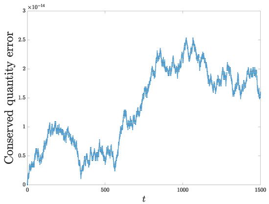
Figure 1. Errors in the conserved quantity I for Example 1 with $h=0.1$.

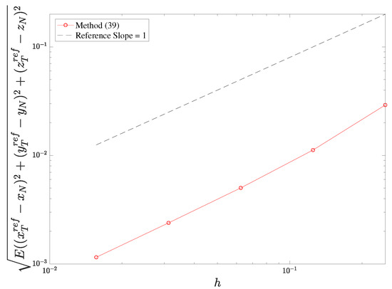
Figure 2. Convergence order for Example 1.

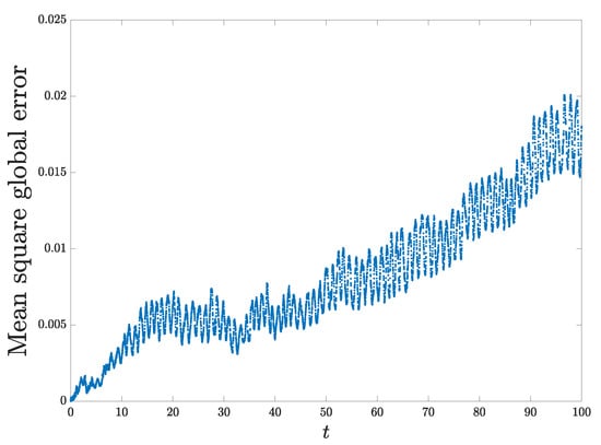
Figure 3. Global mean square errors for Example 1 with $h=0.1$.

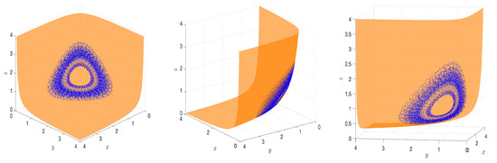
Figure 4. Phase space plot of the numerical solutions from different angels for Example 1 with $h=0.1$.

Example 2.

The stochastic mathematical pendulum.

Consider the following stochastic mathematical pendulum

$$\left\{\begin{array}{c}d\left(\begin{array}{c}p\left(t\right)\\ q\left(t\right)\end{array}\right)=\left(\begin{array}{c}-sin\left(q\right(t\left)\right)\\ p\left(t\right)\end{array}\right)(dt+\beta \circ dW\left(t\right)),\hfill \\ p\left(0\right)=p_0,q\left(0\right)=q_0,\hfill \end{array}\right.$$

(40)

where $\beta$ is a constant denoting the noise intensity. This single-integrand conservative SDE is a stochastic canonical Hamiltonian system. The Hamiltonian $H(p,q)={\displaystyle \frac{p^2}{2}}-cosq$, also known as the energy function, is the conserved quantity.

We employ the CSSRK method (26) with (37), which satisfies the conditions of being conservative and of mean square convergence order 2; that is,

$$\begin{array}{c}{Y}_{\tau }=y_0+\mu \left(h\right){\int }_0^1(4\tau -6\tau \xi -3{\tau }^2+6{\tau }^2\xi )f\left(Y_{\xi }\right)d\xi ,\hfill \\ y_1=y_0+\mu \left(h\right){\int }_0^{1}f\left(Y_{\xi }\right)d\xi .\hfill \end{array}$$

(41)

We take the step size $h=0.01$, the constant $\beta =0.1$, and the initial values $p_0=0,q_0=0.5$. A quadrature formula of order 4 is used in the implementation of the experiment.

Figure 5 exhibits the errors in the conserved quantity $H(p,q)$ according to the CSSRK method (41) on the interval $[0,500]$, where we can see the method is successfully preserving the conserved quantity. Figure 6 demonstrates the convergence order, where 1000 independent sample paths and five different step sizes $h=2^{-2},2^{-3},2^{-4},2^{-5},2^{-6}$ are adopted, as in the previous example. The mean square errors at the terminal $T=1$ are estimated by $\sqrt{\left({\displaystyle \sum _{i=1}^{1000}}\left(\right|p(1,{\omega }_i)-p_N\left({\omega }_i\right){|}^2+|q(1,{\omega }_i)-q_N\left({\omega }_i\right){|}^2)\right)/1000}$, and the results are shown in Figure 6, where we can observe that the convergence order is 2 as expected. Figure 7 reports the global mean square errors on the interval $[0,100]$. Figure 8 plots a numerical sample path of the CSSRK method (41) on the interval $[0,500]$.

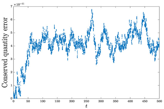
Figure 5. Errors in the conserved quantity H for Example 2 with $h=0.01$.

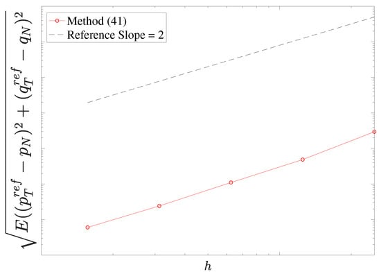
Figure 6. Convergence order for Example 2.

Figure 7. Global mean square errors for Example 2 with $h=0.01$.

Figure 8. Phase space plot of the numerical solutions for Example 2 with $h=0.01$.

6. Conclusions and Remarks

In this paper, we studied the conservative CSSRK methods for solving SDEs. Firstly, we presented the CSSRK methods and investigated the order conditions via the stochastic B-series theory. Secondly, we provided the sufficient conditions in terms of the coefficients of the CSSRK methods, as well as the coefficients of the polynomials for preserving the conserved quantity of SDEs. It turns out that the derived conservative conditions in terms of the coefficients of the polynomials are very easy to use. Then, we constructed conservative CSSRK methods of mean square convergence order 1 in various cases for general conservative SDEs, as well as conservative CSSRK methods of high order for single-integrand conservative SDEs. Notably, for the numerical simulation of conservative SDEs, most of the existing conservative methods are of low convergence order; here, we construct a high-order conservative method easily realized for single-integrand conservative SDEs. Finally, we provide some remarks and future work concerning this paper.

(i)

In our construction of conservative CSSRK methods of mean square convergence order 1, we find the known stochastic averaged vector field method is a special case of the derived conservative CSSRK methods. It seems that CSSRK methods may have promising applications in constructing structure-preserving numerical methods.

(ii)

It should be pointed out that we restrict ourselves to the case that the degree of $\xi$ is one less than that of $\tau$ in $A_{\tau ,\xi }$ and ${\tilde{A}}_{\tau ,\xi }^{r,k}$ when proving the conservative conditions for CSSRK methods. A further investigation for other cases is of interest in our future work.

(iii)

In this paper, we have only considered conservative SDEs with a single conserved quantity. On the other hand, some SDEs possess multiple conserved quantities. Hence, based on the results in this paper, we would proceed to study CSSRK methods for SDEs, leaving multiple conserved quantities numerically invariant.

References

- Mao, X. Stochastic Differential Equations and Their Applications; Horwood: New York, NY, USA, 1997. [Google Scholar]
- Milstein, G.N. Numerical Integration of Stochastic Differential Equations; Kluwer Academic Publishers: Dordrecht, The Netherlands, 1995. [Google Scholar]
- Brugnano, L.; Calvo, M.; Montijano, J.I.; Rández, L. Energy-preserving methods for Poisson systems. J. Comput. Appl. Math. 2012, 236, 3890–3904. [Google Scholar] [CrossRef]
- Celledoni, E.; McLachlan, R.I.; McLaren, D.I.; Owren, B.; Quispel, G.R.W.; Wright, W.M. Energy preserving Runge-Kutta methods. ESAIM Math. Model. Numer. Anal. 2008, 43, 645–649. [Google Scholar] [CrossRef]
- Cohen, D.; Hairer, E. Linear energy-preserving integrators for Poisson systems. BIT Numer. Math. 2011, 51, 91–101. [Google Scholar] [CrossRef]
- Hairer, E. Energy-preserving variant of collocation methods. J. Numer. Anal. Indust. Appl. Math. 2010, 5, 73–84. [Google Scholar]
- McLachlan, R.I.; Quispel, G.R.W.; Robidoux, N. Geometric integration using discrete gradients. Phil. Trans. R. Soc. A 1999, 357, 1021–1045. [Google Scholar] [CrossRef]
- Miyatake, Y. An energy-preserving exponentially-fitted continuous stage Runge-Kutta method for Hamiltonian systems. BIT Numer. Math. 2014, 54, 777–799. [Google Scholar] [CrossRef]
- Miyatake, Y.; Butcher, J.C. A characterization of energy-preserving methods and the construction of parallel integrators for Hamiltonian systems. SIAM J. Numer. Anal. 2016, 54, 1993–2013. [Google Scholar] [CrossRef]
- Quispel, G.R.W.; McLaren, D.I. A new class of energy-preserving numerical integration methods. J. Phys. A Math. Theor. 2008, 41, 045206. [Google Scholar] [CrossRef]
- Iavernaro, F.; Pace, B. s-stage trapezoidal methods for the conservation of Hamiltonian functions of polynomial type. AIP Conf. Proc. 2007, 936, 603–606. [Google Scholar]
- Brugnano, L.; Iavernaro, F.; Trigiante, D. Hamiltonian boundary value methods: Energy preserving discrete line integral methods. J. Numer. Anal. Indust. Appl. Math. 2010, 5, 17–37. [Google Scholar]
- Amodio, P.; Brugnano, L.; Iavernaro, F. A note on the continuous-stage Runge-Kutta(-Nyström) formulation of Hamiltonian Boundary Value Methods (HBVMs). Appl. Math. Comput. 2019, 363, 124634. [Google Scholar] [CrossRef]
- Tang, Q.; Chen, C. Continuous finite element methods for Hamiltonian systems. Appl. Math. Mech. 2007, 28, 1071–1080. [Google Scholar] [CrossRef]
- Tang, W.; Sun, Y. Time finite element methods: A unified framework for numerical discretizations of ODEs. Appl. Math. Comput. 2012, 219, 2158–2179. [Google Scholar] [CrossRef]
- Tang, W.; Sun, Y. A new approach to construct Runge-Kutta type methods and geometric numerical integrators. AIP Conf. Proc. 2012, 1479, 1291–1294. [Google Scholar]
- Tang, W.; Sun, Y. Construction of Runge-Kutta type methods for solving ordinary differential equations. Appl. Math. Comput. 2014, 234, 179–191. [Google Scholar] [CrossRef]
- Wu, X.; Wang, B.; Shi, W. Efficient energy-preserving integrators for oscillatory Hamiltonian systems. J. Comput. Phys. 2013, 235, 587–605. [Google Scholar] [CrossRef]
- Mei, L.; Huang, L.; Wu, X. Energy-preserving continuous-stage exponential Runge-Kutta integrators for efficiently solving Hamiltonian systems. SIAM J. Sci. Comput. 2022, 44, A1092–A1115. [Google Scholar] [CrossRef]
- Misawa, T. Energy conservative stochastic difference scheme for stochastic Hamilton dynamical systems. Jpn. J. Ind. Appl. Math. 2000, 17, 119–128. [Google Scholar] [CrossRef]
- Hong, J.; Zhai, S.; Zhang, J. Discrete gradient approach to stochastic differential equations with a conserved quantity. SIAM J. Numer. Anal. 2011, 49, 2017–2038. [Google Scholar] [CrossRef]
- Li, X.; Zhang, C.; Ma, Q.; Ding, X. Discrete gradient methods and linear projection methods for preserving a conserved quantity of stochastic differential equations. Int. J. Comput. Math. 2018, 95, 2511–2524. [Google Scholar] [CrossRef]
- Wang, Z.; Ma, Q.; Ding, X. Numerical simulations of stochastic differential equations with multiple conserved quantities by conservative methods. East Asian J. Appl. Math. 2022, 12, 53–71. [Google Scholar] [CrossRef]
- Zhou, W.; Zhang, L.; Hong, J.; Song, S. Projection methods for stochastic differential equations with conserved quantities. BIT Numer. Math. 2016, 56, 1497–1518. [Google Scholar] [CrossRef]
- Chen, C.; Hong, J.; Jin, D. Modified averaged vector field methods preserving multiple invariants for conservative stochastic differential equations. BIT Numer. Math. 2020, 60, 1–41. [Google Scholar] [CrossRef]
- Cohen, D.; Dujardin, G. Energy-preserving integrators for stochastic Poisson systems. Commun. Math. Sci. 2014, 12, 1523–1539. [Google Scholar] [CrossRef]
- Butcher, J.C. An algebraic theory of integration methods. Math. Comp. 1972, 26, 79–106. [Google Scholar] [CrossRef]
- Butcher, J.C. Coefficients for the study of Runge-Kutta integration processes. J. Austral. Math. Soc. 1963, 3, 185–201. [Google Scholar] [CrossRef]
- Burrage, K.; Burrage, P.M. Order conditions of stochastic Runge-Kutta methods by B-series. SIAM J. Numer. Anal. 2000, 38, 1626–1646. [Google Scholar] [CrossRef]
- Debrabant, K.; Kværnø, A. B-series analysis of stochastic Runge-Kutta methods that use an iterative scheme to compute their internal stage values. SIAM J. Numer. Anal. 2008, 47, 181–203. [Google Scholar] [CrossRef]
- Komori, Y.; Mitsui, T.; Sugiura, H. Rooted tree analysis of the order conditions of ROW-type scheme for stochastic differential equations. BIT Numer. Math. 1997, 37, 43–66. [Google Scholar] [CrossRef]
- Rößler, A. Rooted tree analysis for order conditions of stochastic Runge-Kutta methods for the weak approximation of stochastic differential equations. Stoch. Anal. Appl. 2006, 24, 97–134. [Google Scholar] [CrossRef]
- Debrabant, K.; Kværnø, A. Cheap arbitrary high order methods for single integrand SDEs. BIT Numer. Math. 2017, 57, 153–168. [Google Scholar] [CrossRef]
- Cohen, D.; Debrabant, K.; Rößler, A. High order numerical integrators for single integrand Stratonovich SDEs. Appl. Numer. Math. 2020, 158, 264–270. [Google Scholar] [CrossRef]
- Xin, X.; Qin, W.; Ding, X. Continuous stage stochastic Runge-Kutta methods. Adv. Differ. Equ. 2021, 2021, 61. [Google Scholar] [CrossRef]
- Tang, W. A note on continuous-stage Runge-Kutta methods. Appl. Math. Comput. 2018, 339, 231–241. [Google Scholar] [CrossRef]
Disclaimer/Publisher’s Note: The statements, opinions and data contained in all publications are solely those of the individual author(s) and contributor(s) and not of MDPI and/or the editor(s). MDPI and/or the editor(s) disclaim responsibility for any injury to people or property resulting from any ideas, methods, instructions or products referred to in the content. |
© 2023 by the authors. Licensee MDPI, Basel, Switzerland. This article is an open access article distributed under the terms and conditions of the Creative Commons Attribution (CC BY) license (https://creativecommons.org/licenses/by/4.0/).