Article

On the Validation of a Fractional Order Model for Pharmacokinetics Using Clinical Data

by
Sinenhlanhla Mtshali
* and
Byron A. Jacobs
Department of Mathematics and Applied Mathematics, University of Johannesburg, Auckland Park, P.O. Box 524, Johannesburg 2006, South Africa
*
Author to whom correspondence should be addressed.
Fractal Fract. 2023, 7(1), 84; https://doi.org/10.3390/fractalfract7010084
Submission received: 1 December 2022 / Revised: 20 December 2022 / Accepted: 9 January 2023 / Published: 11 January 2023
(This article belongs to the Section General Mathematics, Analysis)

Abstract

:
This study aims to validate the hypothesis that the pharmacokinetics of certain drug regimes are better captured using fractional order differential equations rather than ordinary differential equations. To support this research, two numerical methods, the Grunwald–Letnikov and the L1 approximation, were implemented for the two-compartment model with Michaelis–Menten clearance kinetics for oral and intravenous administration of the drug. The efficacy of the numerical methods is verified through the use of the method of manufactured solutions due to the absence of an analytic solution to the proposed model. The model is derived from a phenomenological process leading to a dimensionally consistent and physically meaningful model. Using clinical data, the model is validated, and it is shown that the optimal model parameters select a fractional order for the clearance dynamic for certain drug regimes. These findings support the hypothesis that fractional differential equations better describe some pharmacokinetics.

1. Introduction

Pharmacokinetics is the study of the kinetics of drug absorption, distribution, metabolism, and excretion (ADME). Pharmacokinetic models are usually represented in terms of compartmental models. Given that there are limited data for pharmacokinetic studies, the compartment model can quantitatively monitor the drug concentration in the body and interpolate/extrapolate these dynamics. Furthermore, compartment models are widely used to predict the pharmacokinetics of the drug and the development of dosage regimens. Fractional calculus has become popular in compartmental analysis in recent decades. Its popularity is based on the belief that Fractional Calculus may describe various physical phenomena in a better and more flexible way, especially when those phenomena are connected to fractal geometry [1]. However, all those procedures may be questionable since fractional derivatives do not correspond to differentials, and, in fact, they are not real derivatives but mathematical operators [2]. Fractional calculus fails to perform immediate operations, such as the Leibniz rule for derivatives and various composition rules [2,3]. Pharmacokinetic compartment models are generally formulated mathematically as a system of ordinary differential equations (ODE). The “fractionalization” of the ODE system typically obtains the fractional order compartment model. A single ODE is easily fractionalized by changing the derivative on the left-hand side to a fractional order [4]. However, the fractionalization of a multi-compartment is more complex than fractionalized systems of differential equations as it can lead to dimensionally inconsistent and non-phenomenological models when certain properties, such as mass balance, need to be preserved. The multi-compartment model is built on the basis of the outgoing mass flux being an incoming flux into the next compartment. Furthermore, the outgoing flux is defined as a rate of a fractional order. Without violating mass balance, it cannot appear as an incoming flux into another compartment as a rate of a different fractional order [5]. Therefore, it is impossible to fractionalize multi-compartmental systems by simply changing the order of the derivatives on the left-hand side of the ODEs.
Nonetheless, Dokoumetzidis et al. [4] built a new method to fractionalize a multi-compartmental model with the conservation of mass in which they considered the different fractional order transmission process in the body and demonstrated that the fractional model could well describe the pharmacokinetics of amiodarone in the human body. Moreover, Angstmann et al. [6] derived the fractional compartmental model according to a basic physical stochastic process to ensure that the order of the fractional model had physical significance [7]. We will fractionalize our model based on Dokoumetzidis et al. [4] framework and obey the physical stochastic process by Angstmann et al. [6]. Additionally, fractional order compartment models most commonly use the Riemann–Liouville or the Caputo fractional derivative [8]. A major limitation of the fractional order compartment is that it rarely has the exact algebraic or analytical solution, therefore requires a numerical method to solve them. Nevertheless, stable numerical methods are often complex to implement due to the historical dependence of fractional derivative [6]. The major thrust of the algebraic approach in recent years has been to employ a series expansion method that is not based on small parameters [6]. The infinite series expansion provides an exact algebraic solution and, while these solutions cannot be obtained in a closed form, finite truncations have been proposed as approximations to the exact solution [9]. Among the numerical methods, the most straightforward approach is to replace the Riemann–Liouville derivative with the finite truncation of the Grunwald–Letnikov (GL) derivative, where the latter is formally defined as the limit of a discrete operator and it is equivalent to the Riemann–Liouville derivative [6].
This study aims to understand the numerical schemes’ impact, capturing the different drug administration route properties, such as absorption. The numerical schemes presented are validated in the absence of an exact solution using the method of manufactured solutions. Using this established framework, we perform a sensitivity analysis to identify the effect of each parameter in the model. This sensitivity analysis informs the ultimate goal and novel contribution of this work: by fitting the proposed fractional order model to clinical data for two different drug regimes, we validate the hypothesis that fractional order differential equations can describe pharmacodynamics better than ordinary differential equations can.

2. Preliminaries

While the compartmental fractional model implementation occurs using the GL and L1 approximation, it is worth mentioning the Caputo derivative with the classical derivative. The Caputo derivative of a constant is zero, whereas the Riemann–Liouville fractional derivative of a constant is not equal to zero. However, the Caputo fractional-order differential operator cannot transform a non-constant periodic function into a periodic one, regardless of the period [10]. The exact periodic function can not exist in a class of the Caputo fractional-order differential dynamical systems (including the autonomous case) [10]. Moreover, the GL and the RL derivative are equivalent, especially for applications [11]. Additionally, we will perform a sensitivity analysis of the parameters in the model.

2.1. Fractional Calculus

The integral or order α [ 0 , 1 ] of a function f with respect to time variable t is defined as
I 0 t α f ( t ) = 1 Γ ( α ) 0 t f ( τ ) ( t τ ) α 1 d τ ,
where Γ ( α ) is the Gamma function [11]. When the integer value of α = n , n N , the above definition reduces to the well-known notion of the ordinary n-fold integral. Fractional derivatives of the Grunwald–Letnikov, Riemann–Liouville, and the Caputo derivatives are given based on [11].
w j ( α ) = ( 1 ) j α j , w 0 α = 1 ,
The Caputo fractional derivative of order α is defined as
D 0 C t α f ( t ) = 1 Γ ( m α ) 0 t ( t τ ) m α 1 f ( m ) ( τ ) d τ ,
where m 1 α < m Z + . The RL derivative requires that initial conditions and some of the fractional order initial conditions do not provide clear and meaningful interpretations, which makes it impossible to measure. Nonetheless, the Caputo derivative of a constant is equal, which makes this definition of a fractional order derivative superior for most physical processes since the initial conditions for fractional differential equations with the Caputo derivative have the same form as the integer-order differential equation [7,11].
The GL fractional derivative with fractional order α , if f ( t ) C m [ 0 , t ] , is defined by
D 0 G L t α f ( t ) = j = 0 m 1 f ( j ) ( 0 ) t α + j Γ ( α + j + 1 ) + 1 Γ ( m α ) 0 t ( t τ ) m α 1 f ( m ) ( τ ) d τ ,
where m 1 α < m Z + [12].
The original definition of the GL fractional derivative is given in terms of limit, defined as
D 0 G L t α f ( t ) = lim h 0 1 h α j = 0 ( 1 ) j α j f ( t j h )
Further, the Laplace transform is a useful tool for simplifying a fractional differential equation; however, due to the linearity of the Laplace transform, this process is only amenable to linear fractional differential equations:
L { D a C t α f ( t ) } = s α f ^ ( s ) s α 1 f ( 0 ) ,
where f ^ ( s ) is the Laplace of f ( t ) and 0 < α 1 .

2.2. Fractional Order Compartment Model

The derivation of fractional order compartment models was presented in [13,14,15] by Angstmann et al. We follow the approach presented therein to derive a phenomenological fractional order two-compartment model with Michaelis–Menten clearance dynamics. We assume that the continuous waiting time distribution (non-Markovian waiting time) is a Mittag–Leffler distribution. This distribution has a power–law asymptotic decay [16] expressed as t i.e., ϕ ( t ) t 1 α . The survival function can be expressed as
Φ ( t ) = E α , 1 t τ α ,
0 < α 1 and the time scale parameter as τ > 0 . The Laplace transform of the memory kernel is
L K ( t ) = τ α s 1 α
The Laplace transform of the fractional derivative may be expressed as
L { D 0 t 1 α g ( t ) } = s 1 α L { g ( t ) } 0 D t 1 α g ( t ) | t = 0 ,
based on the generalised definition of the Riemann–Liouville fractional derivation of order 1 α for 0 < α < 1 ,
D 0 t 1 α g ( t ) = 1 Γ ( α ) 0 t f ( t 0 ) ( t t 0 ) 1 α d t 0 ,
where the fractional integral initial condition 0 D t 1 α g ( t ) | t = 0 will be zero for any sufficiently well behaved function [6]. Given that Mittag–Leffler is the time distribution, we have
0 t K ( t t 0 ) x ( t 0 ) e t 0 t μ ( s ) d s d t = τ 0 α D t 1 α x ( t 0 ) e t 0 t μ ( s ) d s ,
where Θ i , j ( t , t 0 ) = exp t 0 t μ ( s ) d s , represent the Markovian function and μ is the time dependent hazard rate. Therefore the general master equation can be written as
d x ( t ) d t = Q ( t ) μ ( t ) x ( t ) τ α x ( t ) e t 0 t μ ( s ) d s 0 D t 1 α x ( t ) e t 0 t μ ( s ) d s ,
which is the general form of the evolution equation for a fractional order compartment model.

2.3. Sensitivity Analysis

Mathematical models have mostly been used to investigate physical phenomena where some parameters could not be known or were not available, which may raise some concerns about the integrity of the parameters. As a result, sensitivity analysis have become a useful tool. Consider the ordinary differential equation (ODE) system
y ( t ) = f ( t , y ; p ) , y ( 0 ) = y 0 ,
with y R and p = { p 1 , p 2 . . . . . . . . ˙ , p k } . Equation (13) is solved using different parameter values and the sensitivity coefficients are calculated [17]. For example, the first order sensitivity to the k t h parameter p k is
y ( t ) p k y ( t , p k + p k ) y ( t , p k ) p k ,
with all other parameters fixed [17].

3. Methodology

We consider a multi-compartment fractional model, illustrated in Figure 1. In this study, we are interested in both model 1, intravenous (IV) bolus, and model 2, oral administration dosage, routes. We will solve both model 1 and model 2 using the standard GL approximation, the L1 approximation. The standard definition is utilized to obtain the numerical solution; nonetheless, it is an unstable numerical scheme for solving FDE regardless of whether a finite difference method is explicit or implicit. Further, the L1 approximation as a discretization method for FDE can lead to an unconditionally stable algorithm.

3.1. Model 1: Intravenous Bolus

The system illustrated by Figure 1a results in a system of a fractional order differential (FDE) equation given by Equations (15) and (16)
d C 1 d t = k 21 C 2 k 12 C 1 V m C 1 V 1 ( K m + C 1 ) ,
where k 12 is the transfer rate of a drug from the central compartment C 1 (mg/L) to the peripheral compartment C 2 (mg/L), k 12 can be represented as k 12 = Q V 1 with Q being the inter-compartment clearance between the central and peripheral compartments (L/h) and V 1 the drug volume distribution from the central compartment (L), and k 21 is the degradation rate in the peripheral compartment (1/h). Further, k 21 can be shown as k 21 = Q V 2 with V 2 being the drug volume from the peripheral compartment (L). Additionally, V m represents the maximum rate of elimination (mg/h) and K m is the Michaelis–Menten constant (mg/L). The nonlinear Michaelis–Menten equation is included to account for the enzyme kinetics in the central compartment.
d C 2 d t = k 12 C 1 k 21 C 2
The system of an ordinary differential equation (ODE) is fictionalized as shown in [4] where the ODE system is integrated and the integrals are fictionalized, and the fractional integral equations are differentiated in an ordinary way. The resulting fractional system contains an ordinary derivative on the left hand side and Riemann–Liouville derivativeson the right hand side [18]. Therefore, the system is formatted mathematically as:
d C 1 d t = θ ( t , 0 ) k 21   D 0 t 1 α C 2 θ ( t , 0 ) k 12 C 1 V m C 1 V 1 ( K m + C 1 ) , d C 2 d t = k 12 C 1 θ ( t , 0 ) k 21   D 0 t 1 α C 2 θ ( t , 0 ) ,
with the initial condition C 1 ( t 0 ) = D V 1 and C 2 ( t 0 ) = 0 .
The linear case of the Equation (17) is solvable by applying the linear Laplace transform given by Equation (6) however, the Michaelis–Menten equation is nonlinear; therefore the Laplace transform property cannot solve Equation (17). Nonetheless, studies such as [4,7,18] have followed the Laplace transform property to the FDE.

3.2. Numerical Algorithm

3.2.1. The Grunwald–Letnikov

We will focus on the finite difference method based on the GL approximate formula and L 1 formula, which are proposed to solve Equation (17) with its initial conditions. First, let t k = k τ , k = 0 , 1 , 2 , , N where N is a positive integer, τ = T / N is the time step and T is the simulation time. The approximation follows the forward-Euler difference method
d C i ( t ) d t | t k τ 1 [ C i ( t k + 1 ) C i ( t k ) ] , i = 1 , 2
Second, using Equation (5) we can obtain the following:
D 0 C t 1 α C 2 ( t ) | t k τ ( 1 α ) j = 0 k w j ( 1 α ) C 2 ( t k j ) ,
Lastly, we can express Equation (17) in terms of the finite difference scheme using the GL approximate formula
C 1 ( t k + 1 ) C 1 ( t k ) τ = k 21 τ ( 1 α ) j = 0 k w j ( 1 α ) C 2 ( t k j ) k 12 C 1 ( t k ) V m C 1 ( t k ) V 1 ( K m + C 1 ( t k ) ) , C 2 ( t k + 1 ) C 2 ( t k ) τ = k 12 C 1 ( t k ) k 21 τ ( 1 α ) j = 0 k w j ( 1 α ) C 2 ( t k j ) ,

3.2.2. L1 Approximation

For simplicity, we can express the L1 approximation as
D 0 C t α f ( t ) t = t n + 1 / 2 = b 0 2 ( f ( t n + 1 ) + f ( t n ) ) 1 2 j = 1 n ( b n j b n j + 1 ) ( f ( t j 1 ) + f ( t j ) ) 1 2 ( b n B n ) ( f ( t 0 ) + f ( t 1 ) ) B n f ( t 0 ) + O ( t 2 α ) ,
where
b n = t α Γ ( 2 α ) ( n + 1 ) 1 α n 1 α , B n = 2 t α Γ ( 2 α ) ( n + 1 / 2 ) 1 α n 1 α
full details are obtained from [19].
Following the L1 formula in [19] we can substitute the shift GL formula
D 0 C t 1 α C 2 | t k t α Γ ( 2 α ) b 0 ( α ) C 2 ( t k ) i = 1 k 1 b k i 1 α b k i α C 2 ( t k ) b k 1 α C 2 ( t 0 ) ,
where b l ( α ) = ( k + 1 ) ( 1 α ) k ( 1 α ) , k 0 . Further, we can establish another finite difference scheme for this problem
C 1 ( t k + 1 ) C 1 ( t k ) τ = k 21 τ ( 1 α ) Γ ( 1 + α ) b 0 ( α ) C 2 ( t k ) i = 1 k 1 b k i 1 ( 1 α ) b k i ( 1 α ) C 2 ( t k ) b k 1 ( 1 α ) C 2 ( t 0 ) k 12 C 1 ( t k ) V m C 1 ( t k ) V 1 ( K m + C 1 ( t k ) ) ,
C 2 ( t k + 1 ) C 2 ( t k ) τ = k 21 τ ( 1 α ) Γ ( 1 + α ) b 0 ( α ) C 2 ( t k ) i = 1 k 1 b k i 1 ( 1 α ) b k i ( 1 α ) C 2 ( t k ) b k 1 ( 1 α ) C 2 ( t 0 ) + k 12 C 1 ( t k ) ,

4. Model 2: Oral Absorption

As a second example, we consider the oral absorption illustrated by Figure 1b, which is a variation of the system of Equations (15) and (16). Technically, this is a three-compartment system where the drug is absorbed in the gastrointestinal tract (GI) denoted ( C 3 ), transferred to the central (first) compartment, and finally, to the peripheral (second) compartment. The GI ( C 3 ) compartment is written as
d C 3 d t = k a C 3 , C 3 ( t ) = F D V 1 e ( k a t ) ,
where k a is the absorption rate constant (1/h), F is the bioavailability fraction of the dose, and D is the dose.
The oral absorption model is written as
d C 1 d t = k 21 C 2 k 12 C 1 + k a C 3 V m C 1 V 1 ( K m + C 1 ) , d C 2 d t = k 12 C 1 k 21 C 2
The initial conditions for this system are zeros expressed as C 1 ( t 0 ) = C 2 ( t 0 ) = 0 .
Thus, the fractional three-compartment system with oral absorption is expressed as:
d C 1 d t = θ ( t , 0 ) k 21   D 0 t 1 α C 2 θ ( t , 0 ) k 12 C 1 + F D V 1 e ( k a t ) V m C 1 V 1 ( K m + C 1 ) , d C 2 d t = k 12 C 1 θ ( t , 0 ) k 21   D 0 t 1 α C 2 θ ( t , 0 )

Implementation: The Grunwald–Letnikov and L1 Approximations

The proposed numerical schemes for model 2 will follow the numerical schemes in model 1.
  • The GL Approximate Formula
C 1 ( t k + 1 ) C 1 ( t k ) τ = k 21 τ ( 1 α ) j = 0 k w j ( 1 α ) C 2 ( t k j ) k 12 C 1 ( t k ) + F D V 1 e ( k a t k ) V m C 1 ( t k ) V 1 ( K m + C 1 ( t k ) ) , C 2 ( t k + 1 ) C 2 ( t k ) τ = k 12 C 1 ( t k ) k 21 τ ( 1 α ) j = 0 k w j ( 1 α ) C 2 ( t k j )
  • The L1 Approximation
C 1 ( t k + 1 ) C 1 ( t k ) τ = k 21 τ ( 1 α ) Γ ( 1 + α ) b 0 ( α ) C 2 ( t k ) i = 1 k 1 b k i 1 ( 1 α ) b k i ( 1 α ) C 2 ( t k ) b k 1 ( 1 α ) C 2 ( t 0 ) k 12 C 1 ( t k ) + F D V 1 e ( k a t k ) V m C 1 ( t k ) V 1 ( K m + C 1 ( t k ) ) ,
C 2 ( t k + 1 ) C 2 ( t k ) τ = k 21 τ ( 1 α ) Γ ( 1 + α ) b 0 ( α ) C 2 ( t k ) i = 1 k 1 b k i 1 ( 1 α ) b k i ( 1 α ) C 2 ( t k ) b k 1 ( 1 α ) C 2 ( t 0 ) + k 12 C 1 ( t k ) ,

5. Method of Manufactured Solution

The method of manufactured solution (MMS) is a general procedure that can be used to construct an analytical solution to the differential equation from the basis of the numerical simulation code [20]. The simulation code has to be tested with the MMS test; the simulation code in question provides an unambiguous result that checks whether the algorithm is implemented correctly or not. Further, it is essential for the numerical simulation code to have an exact solution—or at least a reliable solution—to compare the verification with. The MMS procedure follows four steps:
  • A solution is manufactured.
  • The manufactured solution is passed through the governing equation to produce the new source term.
  • The source term undergoes verification by being added to the governing equation.
  • The code is run and compares the numerical solution to the solution manufactured in step 1 [21].
Using the MMS as in [20,21], we validated the GL and L1 numerical methods for this class of problem, ensuring that the methods recovered O ( Δ t ) and O ( Δ t 2 α ) , respectively. We present the approximate solutions for both methods, showing that their dynamics are qualitatively equivalent. This comparison is made to ensure that the numerical methods used do not produce erroneous dynamics.

6. Results

In this section, we give a comparison of the numerical schemes in Section 4 to enhance the understanding of the predictions for single-dose fractional-order pharmacokinetics. We consider the oral and IV bolus administration route. Without violating the mass balance of the compartment model, the ODE system is fractionalized, as mentioned in the earlier sections. In the methods section, we described the PK models: a two-compartment IV bolus single-dose model of Equations (15) and (16), shown schematically in Figure 1a, and the three-compartment oral single-dose model of Equations (26) and (27), shown schematically in Figure 1b. Additionally, we investigated the effect of the fractional order on the PK model. Using the method of manufactured solution, we chose an analytical solution, and then substituted the analytical expression into the three numerical methods.
We will first consider the intravenous bolus model. We utilize the same parameter value k 12 = 0.8 , k 21 = 0.7 , V m a x = 0.1 parameters adopted or obtained from well-established studies, such as Dokoumetizidis [4], and d = 0.04 , V 1 = 0.001 estimated based on the acceptable range.
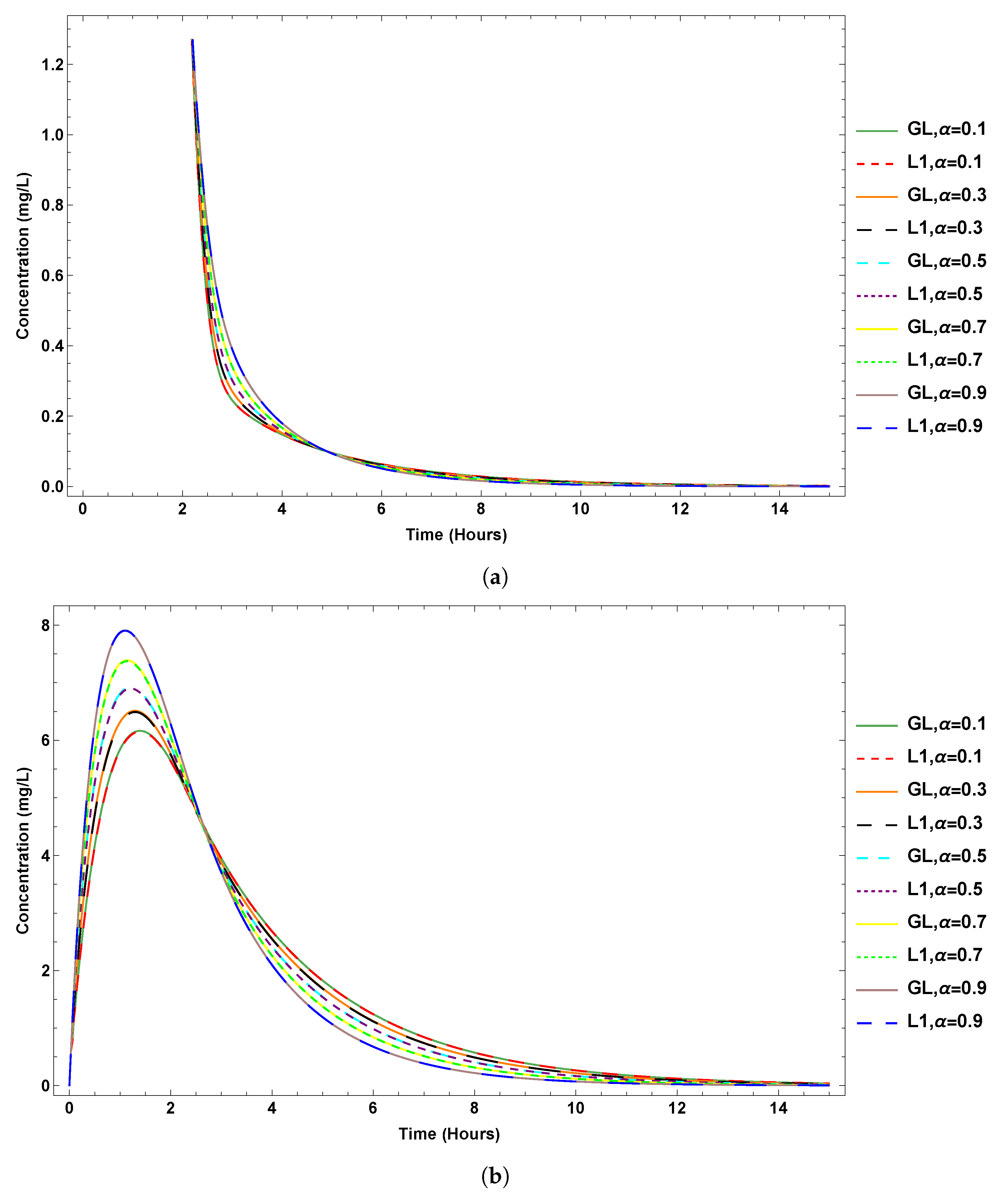
Figure 2 suggests an excellent agreement between the numerical methods. Figure 2a indicates that the concentration of the lower fractional order value, α descends faster than, the higher fractional order value, α .
Further, we consider the oral administration model. Unlike the IV bolus administration process, it is essential that an absorption phase that transfers the drug from the absorption site into the systemic vascular system must occur for an extravascular route such as an oral administration route. Using Dokoumetizidis [4] parameter values; k 12 = 0.6 , k 21 = 0.7 , V m a x = 0.1 , k a = 2 , with d = 1 and V 1 = 0.01 as assumed terms.
We will not pay attention to the gastrointestinal tract compartment results, since they represent flux going out from the gut into the central compartment, indicating that results would be the same regardless of the fractional-order value as illustrated by Figure 3a. Additionally, the process of gastrointestinal absorption is mainly dependent on the physiology and anatomy of the gastrointestinal system and on the physicochemical characteristics of the drug.
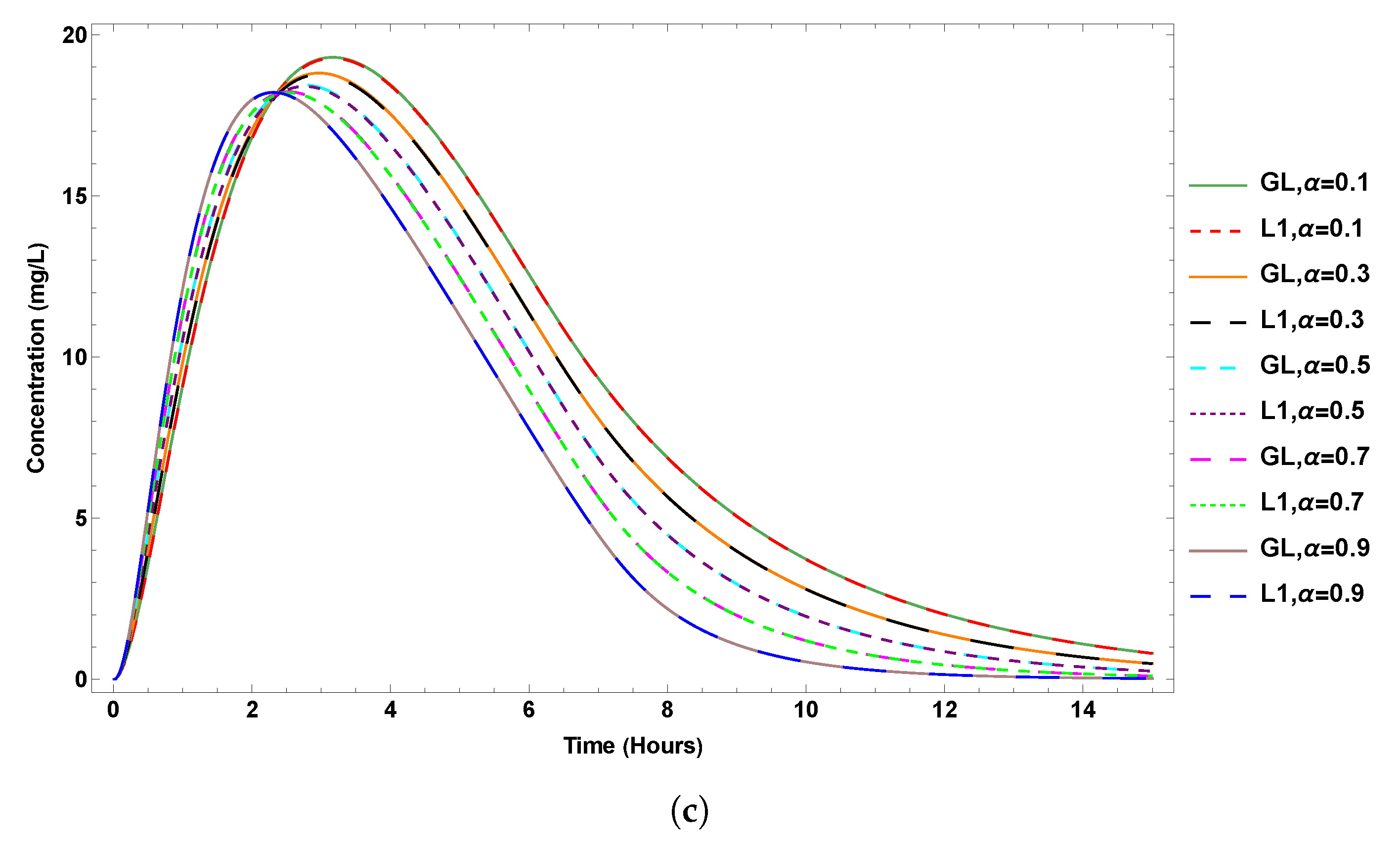
The oral administration route’s central compartment depends on the gut’s flux. However, oral drug bio-availability can easily be influenced by physiological factors, such as the gastrointestinal pH, gastric emptying, small intestinal transit time, and bile salt absorption mechanism [22]. The numerical schemes in the central compartment concentration are similar even though they have different concentration levels, as seen in Figure 3b. Further, Figure 3b indicates that the concentration descends faster for lower fractional order values of α . This suggests that the drug’s excretion or elimination occurs for the intravenous bolus model. Moreover, we can see the excellent agreement between the two numerical methods seen in Figure 3.

7. Sensitivity Analysis

We performed the sensitivity analysis to observe how uncertain our models’ parameters were. The sensitivity analysis follows Section 1, where we chose P to be equal to 10% of the original parameter value.
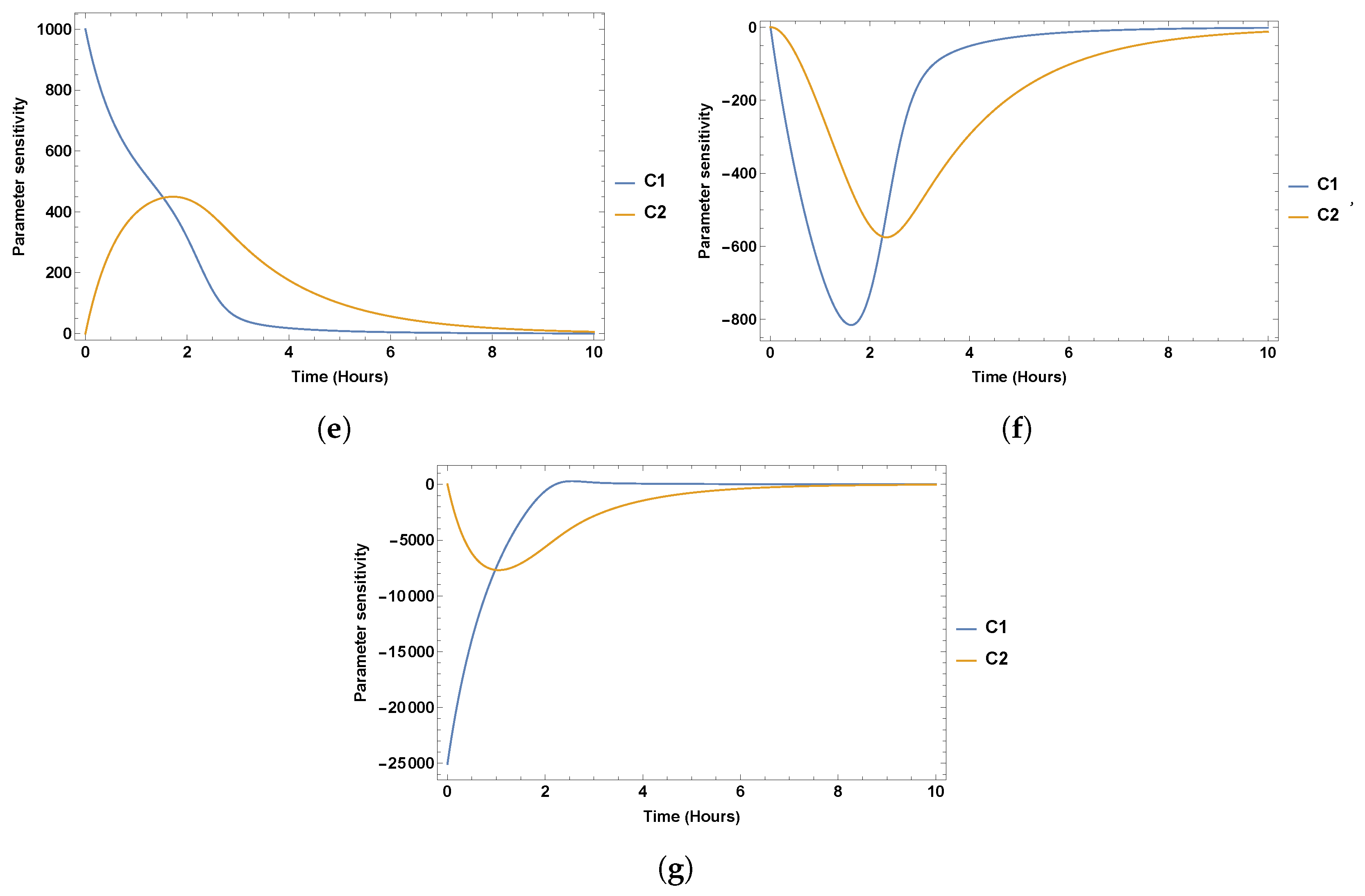
The dose, D, indicates some level of sensitivity in the central compartment. As mentioned earlier, the administration of an IV bolus enters the central compartment, and drug distribution is instantaneous. The drug may move to the peripheral compartment. Further, k 21 suggests some sensitivity to the peripheral compartment as well. The fractional-order alpha exhibits the memory effect dynamic not captured adequately by the other parameters as shown in Figure 4.
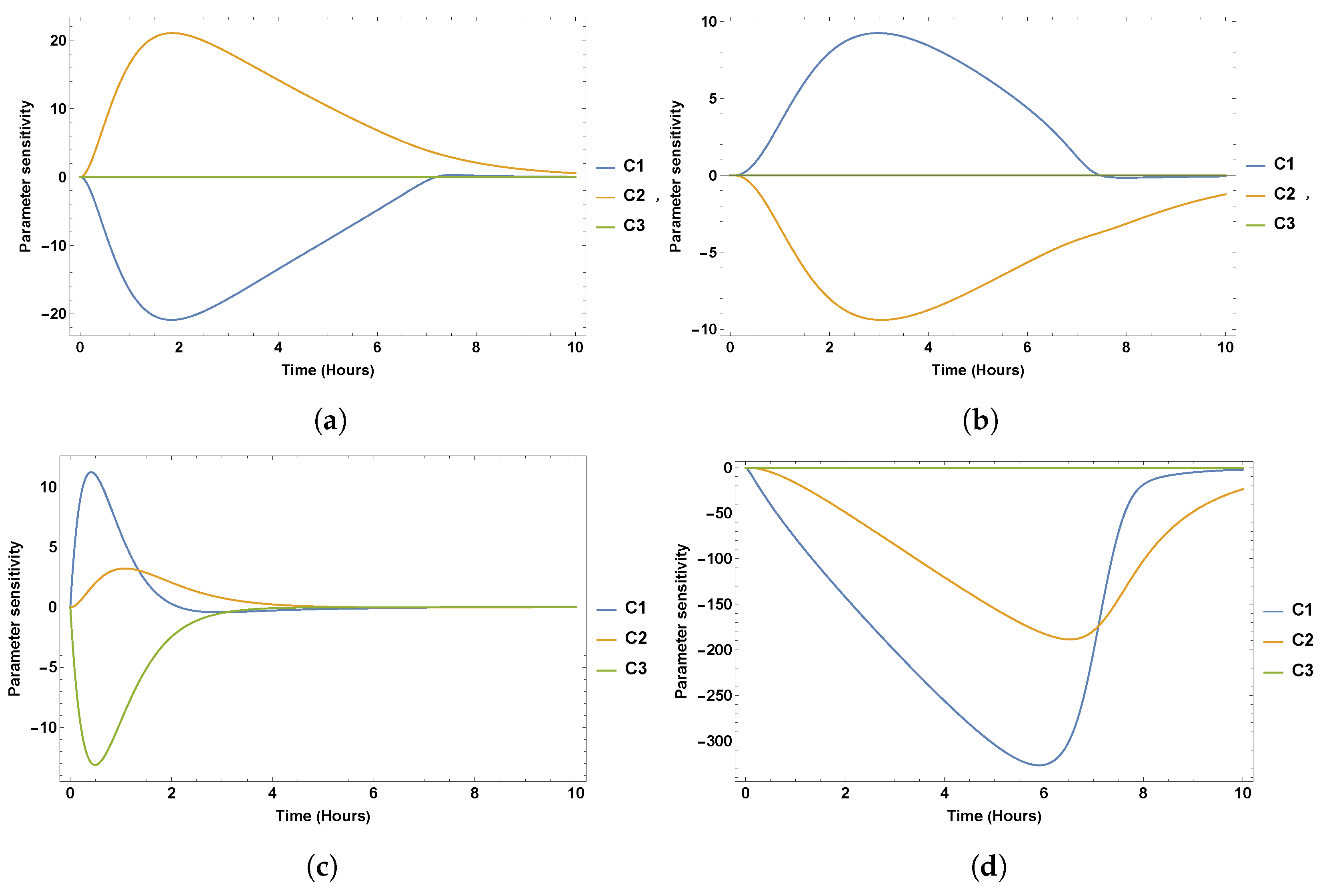
Lastly, we consider the parameter sensitivity of the oral administration model. The bioavaliablity fraction, F and the dose, D, follow the same pattern. Both the F and D are obtained in the initial condition, indicated by Figure 5f,h. Further, the maximum rate of elimination, V m and the Michaelis–Menten constant, K m , exhibit the same pattern but have the opposite signs. These parameters are part of the Michaelis–Menten function as shown in Figure 5d,e. An oscillatory behaviour of fractional-order, α , is observed.

Clinical Data

This section will only analyse the oral route model since the clinical data administration route was oral. By employing the conjugate gradient (CG) method, we optimised the model parameters to fit the clinical data. The CG method is the most well-known iterative method for solving sparse systems of linear equations [23]. We introduced stochasticity into the conjugate gradient method, which allowed us to run the numerical scheme multiple times. We ran the simulations ten times for a single day and determined the standard error of the mean of the clinical data and literature parameter values. Additionally, for the interest of this study, we will not pay attention to the implications of drug co-administration.
The clinical study follows the methodology applied in [24] whereby they compared the steady-state pharmacokinetics of lopinavir (LPV) and ritonavir (RTV) using noncompartmental analysis under 4 sequential treatment conditions over a 12-h dosing interval in HIV-infected participants: a standard dose of LPV/RTV (400 mg/100 mg) every 12 h (study day 1), after which rifampin at 600 mg daily was commenced; LPV/RTV in standard doses every 12 h with rifampin (study day 8); 1.5 times the standard dose of LPV/RTV (600 mg/150 mg) every 12 h with rifampin (study day 15); and twice the standard dose of LPV/RTV (800 mg/200 mg) every 12 h with rifampin (study day 22).
The Day 1 optimal solution for LPV was 4.37869, while RTV’s optimal solution was 0.820684. Day 1 of the clinical trial uses the standard dose with no co-administration of rifampin. Further, the optimal solution decreased for Day 8 and Day 15 when LPV and RTV were co-administered with 600 mg rifampin. For Day 2, the optimal solution for LPV co-administered with rifampin became 1.67261, while the RTV + rifampin became 0.429293. Additionally, for day 15, there was a slight increase in the optimal solution whereby the optimal solution for LPV + rifampin was 1.87927, and RTV + rifampin was 0.5805. This increase may be due to the standard dose being increased by 1.5 times. Lastly, on day 22, the standard dose was doubled with the rifampin dose remaining at 600 mg; we observed that the optimal solution increased and became higher than on day 1 for the co-administration of RTV and rifampin, 1.04898. Nonetheless, for the co-administration of LPV and rifampin, the optimal solution (3.717) increased but remained low compared to Day 1. The low optimal solution indicates that the algorithm converges fast and there are fewer iteration steps required to obtain the solution, while the high optimal solution suggests the opposite.
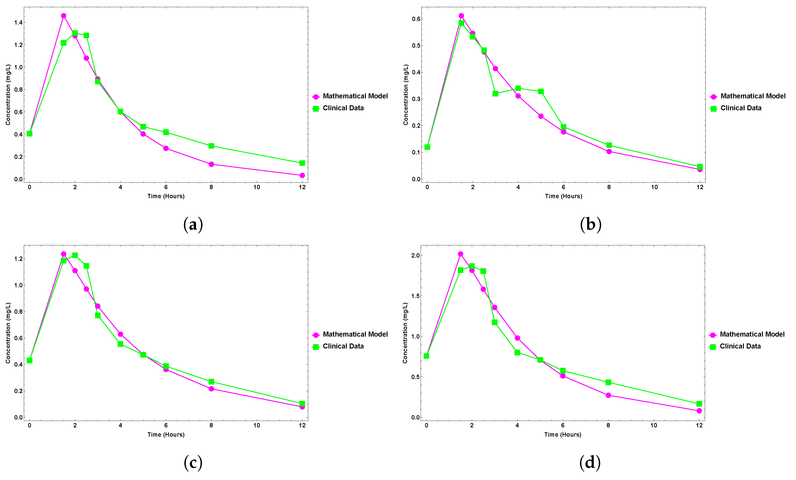
Figure 6a indicates some correlation between the standard dose and co-administration of RTV greater than the standard dose with rifampin. Further, there is a better fit in Figure 6c. Figure 6b appears to be different compared to the other dose measurements; however, the mathematical model and clinical data started at the same measurement and differed after 2.5 h. Furthermore, they followed the same behaviour pattern for approximately 5 h.
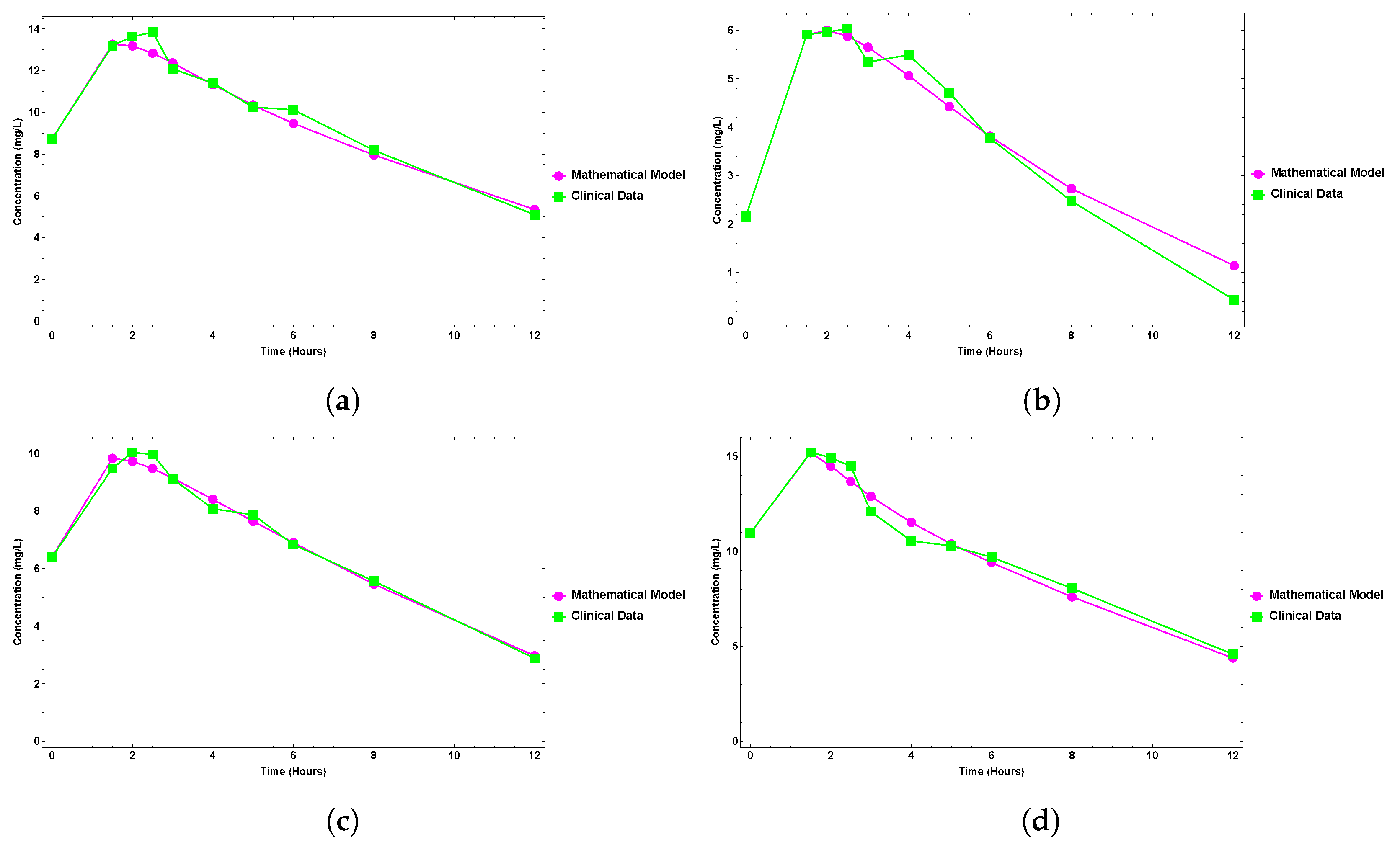
Figure 7 suggests a direct relationship between the different dose measurements, and the fractional model fits well with the lopinavir. However, as observed in Figure 6c, Figure 6c appears to be different compared to the other dose measurements, which suggests that there may be some sensitivity when the standard dose is co-administered with rifampin.
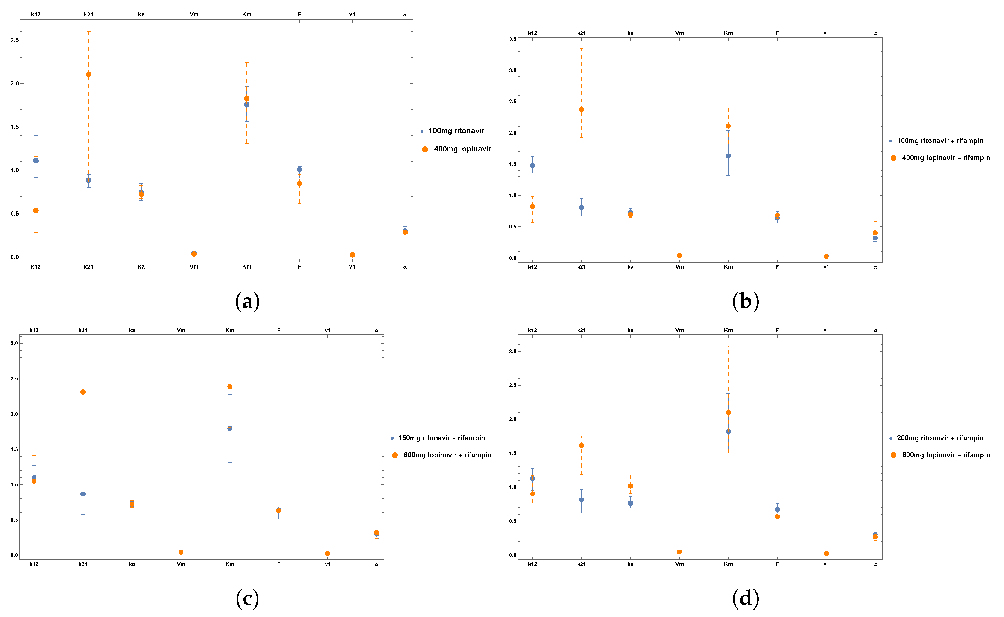
Figure 8 indicates that V m and V 1 had very similar results for all ten runs, which resulted in a significantly low variance for both ritonavir and lopinavir. The variance of lopinavir is higher than that of ritonavir except for bioavailability, F. Figure 8b suggests that the variance of all the other parameters increased except for F; however, F overlaps with the other parameters, indicating no significant differences between the clinical data and mathematical parameters for the ritonavir. However, for the lopinavir, there was a reduction in the parameter value differences among k 12 , k a , and F, while the variance between k 21 and k m increased. Opposite to the observation in Figure 8a, the fractional order, α , increased for lopinavir. Most of the variance in the parameter remained in a similar range for Figure 8b,c; nonetheless, the variance of k m increased, while the k 12 variance decreased for ritonavir. Further, the lopinavir bioavailability, F, value decreased in Figure 8c compared to Figure 8b and reached a constant value throughout all the runs, resulting in no variance. From Figure 6d, we can conclude that as the concentration of ritonavir increases, so does the variance in parameters except for k 21 , which dropped, and the fractional order, α , which remained very similar.
Additionally, with an increase in lopinavir, the parameter variance also decreased. We have looked into the impact of drug co-administration and drug–drug interaction in [25]. Further, there is no variance in Figure 8d. We kept the fractional order, α = 0.5 , constant throughout all of the runs performed, as mentioned at the beginning of this section. Therefore, the fractional order, α , may not have impacted much. The fractional order, α , variance decreased from Figure 8b and remained the same for both Figure 8c,d. Moreover, the variance increased for k 12 , k a , and k m while reducing for k 21 . The parameter variance observed to increase in Figure 8c decreased in Figure 8d, and the variance of k m further decreased.

8. Discussion

Using the Dokoumetzidis et al. [4] framework, we fractionalized the different route fractional order compartment model. The fractionalized model was solved using two numerical schemes, the L1 and GL approximations. The theoretical results were improved by running the numerical simulation. Further, the numerical schemes were validated using the MMS. We then performed sensitivity analysis against all of the model’s parameters and fitted the clinical data with the oral route model. The central compartment included blood and the highly perfused organs and tissues such as the heart, brain, lungs, liver, and kidney. In these organs, the administered drug usually equilibrated rapidly. While the peripheral compartment includes less well-perfused organs such as adipose and skeletal muscle, the administered drug would equilibrate more slowly in these organs. The duration of the drug effect at the target tissue would often be affected by the redistribution from one compartment to another. Moreover, the oral route administration model had an extra gastrointestinal compartment. For most two-compartment models, the elimination occurred from the central compartment model unless other information about the drug was known since the major sites of drug elimination (renal excretion and hepatic metabolism) occurred from organs such as the kidney and liver, which were highly perfused with blood [26], as illustrated by Figure 1. Two fundamental processes describing oral drug absorption includes the dissolution of a drug into GI fluid and the permeation of a dissolved drug through the intestinal wall and into the bloodstream [27]. Further, since the drug medication administered intravenously directly reached the blood circulation, 100% bioavailability was assured. In Section 3, we mentioned that some physiological factors could influence the bioavailability of an oral route drug administration.
From Figure 2a, the steep phase of the curve is called the distribution phase; this is due to the distribution of the drug from the central compartment to the peripheral compartment and the elimination phase. During this phase, the decline of the plasma concentration is associated solely with the elimination of the drug from the body [28]. According to Figure 2a, all fractional values started with the same rapid decline, suggesting the same drug distribution rate from the central compartment to the peripheral. However, the high fractional order values overtook the concentration of low fractional order after four hours in the elimination phase, which suggests that the concentration of high fractional order values is eliminated faster. Figure 3b, suggests both rapid concentration distribution to the peripheral and elimination. Further, the equilibrium in the central compartment of both models is reached relatively quickly and leads to fairly constant drug exposure in the peripheral compartment.
The dose, D, shows some sensitivity to the central compartment ( C 1 ). However, the dose is introduced in the central compartment and distributed to the peripheral compartment ( C 2 ) for the IV bolus model. Further, a similar trend was observed for the oral route administration model where the C 1 and C 2 suggest some sensitivity to the dose, D. Additionally, fraction F has the same result as dose D. The transfer rate, k 12 , and degradation rate, k 21 , indicate no sensitivity and have a similar trend, albeit in the opposite direction. Furthermore, the fractional order is observed to have no impact on the gastrointestinal compartment ( C 3 ), which is to be expected since the parameter is not part of C 3 .
When the standard dose of lopinavir/ritonavir is co-administered with rifampin, we observe a discrepancy between the mathematical model and clinical data. Consequently, following a Food and Drug Administration (FDA) recommendation, this combination should be avoided [29]. In addition and for the same reason, at the standard doses, lopinavir/ritonavir cannot be used concomitantly with rifampicin, although it has been reported that an adjusted dose of lopinavir/ritonavir in combination with therapeutic drug monitoring and monitoring of liver function may allow concomitant use of rifampicin in healthy volunteers [30]. Additionally, we observe minor differences between the mathematical model and the clinical data for the lopinavir/ritonavir double dose with rifampin. Lastly, standard deviation errors indicate that there is no significance.

9. Conclusions

This work investigates the effects of the fractional order of the two numerical methods, the GL and L1 approximations of the two compartmental fractional models, considering both the oral and intravenous bolus drug administration routes under different initial conditions. We determined our model’s exact solution using the method of manufactured solutions and fitted the exact solution into our numerical scheme. Further, we performed a sensitivity analysis for all our parameters. Furthermore, we fitted the oral route mathematical model to the clinical PK data and determined the correlation of the model parameters to clinical data using the conjugate gradient method. The lopinavir clinical data were well-fitted with the mathematical model; however, when we performed an ODE PBPK model, we observed that the ritonavir clinical data were well-fitted with the mathematical model (see [25]). This may suggest that the mathematical model or approach influences a particular drug. Nonetheless, we will have to conduct further investigations to understand the impact of a mathematical model on clinical data or specific drugs. The fractional order value influences the drug concentration in the human body. The sensitivity analysis indicated that the model dynamics were well captured. Lastly, there was no significant difference between the model parameters and clinical data.

Author Contributions

Conceptualization, S.M.; Methodology, S.M.; Software, S.M. and B.A.J.; Validation, S.M. and B.A.J.; Formal analysis, S.M.; Investigation, S.M.; Writing—original draft, S.M.; Writing—review & editing, B.A.J.; Visualization, S.M.; Supervision, B.A.J. All authors have read and agreed to the published version of the manuscript.

Funding

This research was funded by the National Department of Science and Innovation and National Research Foundation (DSI-NRF) CoE-MaSS supported this work.

Acknowledgments

We want to thank Christopher N. Angstmann for offering his insights.

Conflicts of Interest

The authors declare no conflict of interest. The funders had no role in the design of the study; in the collection, analyses, or interpretation of data; in the writing of the manuscript, or in the decision to publish the results.

References

  1. Tatom, F.B. The relationship between fractional calculus and fractals. Fractals 1995, 3, 217–229. [Google Scholar] [CrossRef]
  2. Lazopoulos, K.A.; Lazopoulos, A.K. On the mathematical formulation of fractional derivatives. Prog. Fract. Differ. Appl. 2019, 5, 261–267. [Google Scholar]
  3. Tarasov, V.E. No violation of the Leibniz rule. No fractional derivative. Commun. Nonlinear Sci. Numer. Simul. 2013, 18, 2945–2948. [Google Scholar] [CrossRef] [Green Version]
  4. Dokoumetzidis, A.; Magin, R.; Macheras, P. Fractional kinetics in multi-compartmental systems. J. Pharmacokinet. Pharmacodyn. 2010, 37, 507–524. [Google Scholar] [CrossRef] [PubMed]
  5. Dokoumetzidis, A.; Magin, R.; Macheras, P. A commentary on fractionalization of multi-compartmental models. J. Pharmacokinet. Pharmacodyn. 2010, 37, 203–207. [Google Scholar] [CrossRef]
  6. Angstmann, C.N.; Henry, B.I.; Jacobs, B.A.; McGann, A.V. An explicit numerical scheme for solving fractional order compartment models from the master equations of a stochastic process. Commun. Nonlinear Sci. Numer. Simul. 2019, 68, 188–202. [Google Scholar] [CrossRef]
  7. Qiao, Y.; Xu, H.; Qi, H. Numerical simulation of a two compartmental fractional model in pharmacokinetics and parameters estimation. Math. Methods Appl. Sci. 2021, 44, 11526–11536. [Google Scholar] [CrossRef]
  8. Li, C.; Qian, D.; Chen, Y. On Riemann–Liouville and caputo derivatives. Discret. Dyn. Nat. Soc. 2011, 2011, 562494. [Google Scholar] [CrossRef] [Green Version]
  9. Kumar, P.; Agrawal, O.P. An approximate method for numerical solution of fractional differential equations. Signal Process. 2006, 86, 2602–2610. [Google Scholar] [CrossRef]
  10. Kang, Y.-M.; Xie, Y.; Lu, J.-C.; Jiang, J. On the nonexistence of non-constant exact periodic solutions in a class of the Caputo fractional-order dynamical systems. Nonlinear Dyn. 2015, 82, 1259–1267. [Google Scholar] [CrossRef]
  11. Podlubny, I. Fractional Differential Equations: An Introduction to Fractional Derivatives, Fractional Differential Equations, to Methods of Their Solution and Some of Their Applications; Elsevier: Amsterdam, The Netherlands, 1998. [Google Scholar]
  12. Li, C.; Deng, W. Remarks on fractional derivatives. Appl. Math. Comput. 2007, 187, 777–784. [Google Scholar] [CrossRef]
  13. Angstmann, C.N.; Erickson, A.M.; Henry, B.I.; McGann, A.V.; Murray, J.M.; Nichols, J.A. Fractional order compartment models. SIAM J. Appl. Math. 2017, 77, 430–446. [Google Scholar] [CrossRef] [Green Version]
  14. Angstmann, C.N.; Henry, B.I.; McGann, A.V. A Fractional Order Recovery SIR Model from a Stochastic Process. Bull. Math. Biol. 2016, 78, 468–499. [Google Scholar] [CrossRef] [Green Version]
  15. Angstmann, C.N.; Donnelly, I.C.; Henry, B.I.; Nichols, J.A. A Discrete Time Random Walk Model for Anomalous Diffusion. J. Comput. Phys. 2015, 293, 53–69. [Google Scholar] [CrossRef]
  16. Bateman, H. Higher Transcendental Functions [Volumes I–III]; McGraw-Hill Book Company: Columbus, OH, USA, 1953; p. 1. [Google Scholar]
  17. Rabitz, H.; Kramer, M.; Dacol, D. Sensitivity Analysis in Chemical Kinetics. Annu. Rev. Phys. Chem. 1983, 34, 419–461. [Google Scholar] [CrossRef]
  18. Sopasakis, P.; Sarimveis, H.; Macheras, P.; Dokoumetzidis, A. Fractional calculus in pharmacokinetics. J. Pharmacokinet. Pharmacodyn. 2018, 45, 107–125. [Google Scholar] [CrossRef]
  19. Li, C.; Zeng, F. Numerical Methods for Fractional Calculus; CRC Press: Boca Raton, FL, USA, 2015; p. 24. [Google Scholar]
  20. Shunn, L.; Ham, F. Method of Manufactured Solutions Applied to Variable-Density Flow Solvers. Annual Research Briefs 2007 Center for Turbulence Research. 2007. pp. 155–168. Available online: https://web.stanford.edu/group/ctr/ResBriefs07/14_shunn_pp155_168.pdf (accessed on 1 October 2022).
  21. Brglez, Š. Code verification for governing equations with arbitrary functions using adjusted method of manufactured solutions. Eng. Comput. 2014, 30, 669–678. [Google Scholar] [CrossRef]
  22. Song, N.-N.; Zhang, S.-Y.; Liu, C.-X. Overview of factors affecting oral drug absorption. Asian J. Drug Metab. Pharmacokinet. 2004, 4, 167–176. [Google Scholar]
  23. Shewchuk, J.R. An Introduction to the Conjugate Gradient Method without the Agonizing Pain; Carnegie-Mellon University: Pittsburgh, PA, USA, 1994. [Google Scholar]
  24. Decloedt, E.H.; McIlleron, H.; Smith, P.; Merry, C.; Orrell, C.; Maartens, G. Pharmacokinetics of lopinavir in HIV-infected adults receiving rifampin with adjusted doses of lopinavir-ritonavir tablets. Antimicrob. Agents Chemother. 2011, 55, 3195–3200. [Google Scholar] [CrossRef] [Green Version]
  25. Mtshali, S.; Jacobs, B.A. A Comparative Analysis of Physiologically Based Pharmacokinetic Models for Human Immunodeficiency Virus and Tuberculosis Infections. Antimicrob. Agents Chemother. 2022, 66, e00274-22. [Google Scholar] [CrossRef]
  26. Ahmed, T. Pharmacokinetics of drugs following IV Bolus, IV infusion, and oral administration. In Basic Pharmacokinetic Concepts and Some Clinical Applications; IntechOpen: London, UK, 2015; Volume 10. [Google Scholar]
  27. Martinez, M.N.; Amidon, G.L. A mechanistic approach to understanding the factors affecting drug absorption: A review of fundamentals. J. Clin. Pharmacol. 2002, 42, 620–643. [Google Scholar] [CrossRef] [PubMed] [Green Version]
  28. Unil Université Lausanne. Available online: https://sepia2.unil.ch/pharmacology/parameters/distributioneliminationphase/ (accessed on 18 December 2022).
  29. Grange, S.; Schutz, M.; Schmitt, C.; Riek, M.; Gaudeul-Ehrhart, E. Unexpected hepatotoxicity observed in a healthy volunteer study on the effects of multiple dose rifampicin on the steady-state pharmacokinetics of ritonavir-boosted saquinavir and vice versa. In Proceedings of the Sixth International Workshop on Clinical Pharmacology of HIV Therapy, Montreal, QC, Canada, 28–30 April 2005; Abstract 35. p. 28. [Google Scholar]
  30. La Porte, C.J.L.; Colbers, E.P.H.; Bertz, R.; Voncken, D.S.; Wikstrom, K.; Boeree, M.J.; Koopmans, P.P.; Hekster, Y.A.; Burger, D.M. Pharmacokinetics of adjusted-dose lopinavir-ritonavir combined with rifampin in healthy volunteers. Antimicrob. Agents Chemother. 2004, 48, 1553–1560. [Google Scholar] [CrossRef] [PubMed]
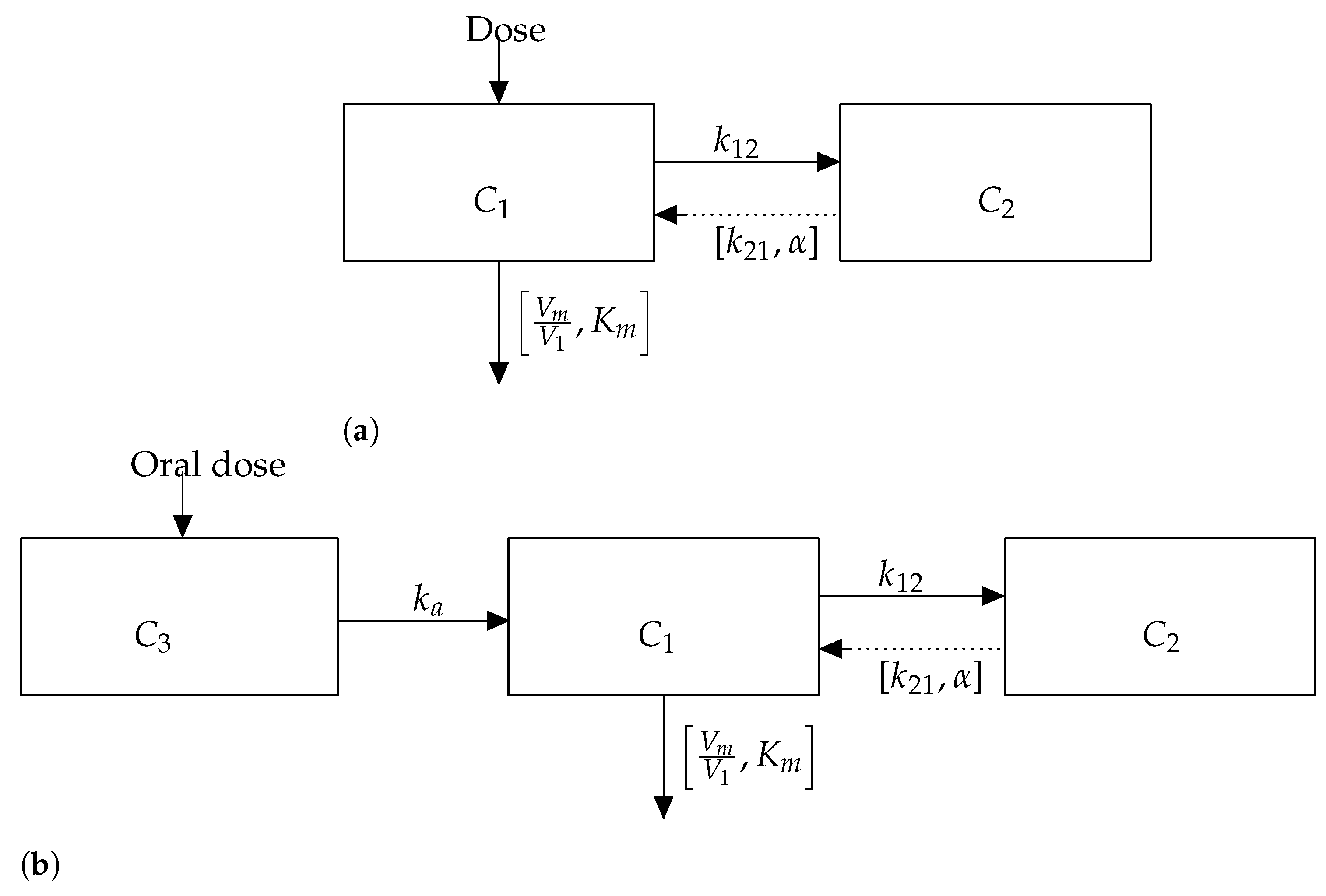
Figure 1. Fractional compartment PK models. First-order absorption and elimination. The flux from the peripheral to the central compartment follows the slower distribution fractional kinetics of the drug, while flux from the central to peripheral compartment follows fast distribution kinetics. The difference in the distribution and redistribution rate is based on the central compartment consisting of the plasma and tissues that distribute the drug instantaneously. In contrast, the peripheral compartment consists of slow distribution. (a) Model 1: The dose is administered in the central compartment as an IV bolus. (b) Model 2: The dose administered orally through the gastrointestinal tract.
Fractalfract 07 00084 g001
Figure 2. The IV bolus administration route model, as a function of time, is fixed, along with several α values. (a) The central compartment concentration. (b) The peripheral compartment concentration.
Fractalfract 07 00084 g002
Figure 3. The oral administration route model, as a function of time, is fixed, along with several α values. (a) The gastrointestinal tract. (b) The central compartment. (c) The peripheral compartment.
Fractalfract 07 00084 g003aFractalfract 07 00084 g003b
Figure 4. IV bolus sensitivity analysis. (a) Transfer rate, k 12 . (b) Degradation rate, k 21 . (c) Michaelis–Menten constant, K m . (d) Fractional order, α . (e) Dose, D. (f) Maximum rate of elimination, V m . (g) Central Volume of distribution, V 1 .
Fractalfract 07 00084 g004aFractalfract 07 00084 g004b
Figure 5. Oral dose sensitivity analysis. (a) Transfer rate, k 12 . (b) Degradation rate, k 21 . (c) Absorption rate constant, k a . (d) Maximum rate of elimination, V m . (e) Michaelis–Menten constant, K m . (f) Dose, D. (g) Central Volume of distribution, V 1 . (h) Bioavaliablity fraction, F. (i) Fractional order, α .
Fractalfract 07 00084 g005aFractalfract 07 00084 g005b
Figure 6. Ritonavir standard dose regimen and co-administration dose regimen. (a) 100 mg ritonavir. (b) 100 mg ritonavir + 600 mg rifampin. (c) 150 mg ritonavir + 600 mg rifampin. (d) 200 mg ritonavir + 600 mg rifampin.
Fractalfract 07 00084 g006
Figure 7. Lopinavir standard dose regimen and Day 4 dose regimen. (a) 400 mg lopinavir. (b) 400 mg lopinavir + 600 mg rifampin. (c) 600 mg lopinavir + 600 mg rifampin. (d) 800 mg lopinavir + 600 mg rifampin.
Fractalfract 07 00084 g007
Figure 8. Different Lopinavir and ritonavir dose regimens with 600 mg rifampin dose. (a) Day one. (b) Day two. (c) Day three. (d) Day four.
Fractalfract 07 00084 g008
Disclaimer/Publisher’s Note: The statements, opinions and data contained in all publications are solely those of the individual author(s) and contributor(s) and not of MDPI and/or the editor(s). MDPI and/or the editor(s) disclaim responsibility for any injury to people or property resulting from any ideas, methods, instructions or products referred to in the content.