Homotopy Analysis Method Analytical Scheme for Developing a Solution to Partial Differential Equations in Fuzzy Environment

Abstract

Partial differential equations are known to be increasingly important in today’s research, and their solutions are paramount for tackling numerous real-life applications. This article extended the analytical scheme of the homotopy analysis method (HAM) to develop an approximate analytical solution for Fuzzy Partial Differential Equations (FPDEs). The scheme used its powerful tools, the auxiliary function and convergence-control parameter, in the analysis and optimization, which ensures the convergence of the approximate series solution in addition to considering all necessary concepts from fuzzy set theory to provide high precision in the fuzzy environment. Furthermore, the efficiency was shown by applying the proposed scheme to linear and nonlinear cases of Fuzzy Reaction–Diffusion Equation (FRDE) and Fuzzy Wave Equation (FWE).

1. Introduction

The fuzziness concept has had growing applications within numerous fields, such as learning theory, automata, decision-making process, algorithms, pattern classification, and linguistics, ever since its commencement [1], and the development of fuzzy derivative by Chang and Zadeh [2], Dubois and Prade used Zadeh’s extension principle [3], Puri and Ralescu [4] suggested to generalize the Hukuhara derivative, Seikkala, as an extension of the Hukuhara derivative [5].

The starting point for the fuzzy differential equation was made by Kandel and Byatt [6,7], Kaleva [8,9], He and Yia [10]. However, when applying either Hukuhara or generalized derivatives into engineering problems, there have been some downsides [11]; the Hukuhara differentiability solution turns inaccurate as time goes by. Bede [12] exhibited that lots of Boundary Value Problems (BVPs) have no solution if the Hukuhara derivative is applied. To remove this difficulty, a generalized Hukuhara derivative was developed in [11,12,13].

These concepts of fuzzy derivative have been opening up a period of applied research of fuzzy mathematics, hence the necessity for attempting different kinds of solutions, including but not limited to: converting the differential equation to a differential inclusion, and the solution is accepted as the α-cut of the fuzzy solution [14], transforming the FDE into equivalent fuzzy integral equation [15], using the Laplace transform method in linear FDE [16], employing the Zadeh extension principle method through solving the associated Differential Equation and then fuzzifying and checking whether the solution is satisfactory [17], and transforming under generalized Hukuhara differentiability the given FDE into two differential equations involving the parametric forms of a fuzzy number [18].

The development of a comprehensive physical equation under the uncertainty of fundamental scientific processes and a variety of social science issues is typically accomplished with the assistance of fuzzy partial differential equations. FPDEs are capable of describing a wide variety of significant dynamical systems that exist in the real world, including fuzzy heat and wave equations. This haziness may manifest itself in each component of a FPDE, including the initial condition, boundary condition, variables, coefficients, and so on. Consequently, the determination of FDEEs in terms of real conditions contributes to the utilization of interval or fuzzy calculations. Buckley and Feuring [19] provided the first definition of a partial differential equation for a fuzzy-valued function. This equation has since been the subject of research in a number of different works.

Numerous approaches have been utilized to construct an exact, approximate analytical and/or numerical solution to FPDEs [20,21,22,23,24,25,26,27,28,29,30,31,32,33,34,35,36,37,38,39]. Despite these efforts, the literature still needs further attention to provide more accurate and capable solutions, mainly for equations that are nonlinear and/or with no exact solution.

Hence, the incentive for our work is to develop an approximate analytical solution using the homotopy analysis method (HAM) developed by Liao as early as 1992 [40]. The method’s ability to deal with nonlinearities comes from using homotopy–Maclaurin series [41], and it overcomes the independence of the existence of perturbation parameters [42]. Furthermore, the technique offers a selection of auxiliary function polynomials or otherwise according to the given problem [43]. In addition, it grants control over the solution rate of convergence and the region of convergence, which is accomplished through introducing an auxiliary function and convergence control parameter to the formulation of the problem [44].

2. The Analytical Scheme Mathematical Formulation

The analytical scheme HAM has been applied to derive an approximate-analytical solution of many kinds of equations [40,41,42,43,44] in a crisp environment. In this section, we shall build our FPDEs proposed solution in a fuzzy environment.

Consider the equation of the following form,

$$\mathcal{N}\left[\tilde{\nu }\left(\mathit{z},t;\alpha \right)\right]=0$$

(1)

where $\mathcal{N}$ is a nonlinear operator, $\tilde{\nu }\left(\mathit{z},t;\alpha \right)$ is an unknown fuzzy function, $\mathit{z}$ denotes an n-dimensional spatial independent variable, and t is an independent temporal variable.

Now, we shall begin by defining the homotopy operator $\mathcal{H}\mathcal{P}\left(\mathit{z},t;p;\alpha \right)$ for all $\alpha \in \left[0, 1\right]$,

$$\mathcal{H}\mathcal{P}\left(\mathit{z},t;p;\alpha \right)=\left(1-p\right)\mathcal{L}\left[\tilde{\theta }\left(\mathit{z},t;p;\alpha \right)-{\tilde{\nu }}_0\left(\mathit{z},t;\alpha \right)\right]-p\tilde{\hslash }\left(\alpha \right)\mathcal{H}\left(\mathit{z},t\right)\mathcal{N}\left[\tilde{\theta }\left(\mathit{z},t;p;\alpha \right)\right]$$

(2)

where $p\in \left[0, 1\right]$ is the embedding parameter that deforms from $0$ to $1$ generating a series solution, $\mathcal{L}$ is an auxiliary linear operator, $\tilde{\theta }\left(\mathit{z},t;p;\alpha \right)$ is an unknown function, ${\tilde{\nu }}_0\left(\mathit{z},t;\alpha \right)$ is a fuzzy initial guess of $\tilde{\nu }\left(\mathit{z},t;\alpha \right)$, $\tilde{\hslash }\left(\alpha \right)\ne 0$ is a convergence-control parameter per each $\alpha$ level set and $\mathcal{H}\left(\mathit{z},t\right)\ne 0$ is an auxiliary function.

Thus, considering $\mathcal{H}\mathcal{P}\left(\mathit{z},t;p;\alpha \right)=0$ yields

$$\left(1-p\right)\mathcal{L}\left[\tilde{\theta }\left(\mathit{z},t;p;\alpha \right)-{\tilde{\nu }}_0\left(\mathit{z},t;\alpha \right)\right]=p\tilde{\hslash }\left(\alpha \right)\mathcal{H}\left(\mathit{z},t\right)\mathcal{N}\left[\tilde{\theta }\left(\mathit{z},t;p;\alpha \right)\right]$$

(3)

which is called the zero-order deformation equation for all $\alpha \in \left[0, 1\right]$.

Now, for $p=0$, Equation (3) gives the deformation,

$$\mathcal{L}\left[\tilde{\theta }\left(\mathit{z},t;0;\alpha \right)-{\tilde{\nu }}_0\left(\mathit{z},t;\alpha \right)\right]=0$$

(4)

$$\tilde{\theta }\left(\mathit{z},t;0;\alpha \right)={\tilde{\nu }}_0\left(\mathit{z},t;\alpha \right)$$

(5)

Then again, for $p=1$, Equation (3) reduces to the deformation,

$$\tilde{\hslash }\left(\alpha \right)\mathcal{H}\left(\mathit{z},t\right)\mathcal{N}\left[\tilde{\theta }\left(\mathit{z},t;1;\alpha \right)\right]=0$$

(6)

$$\tilde{\theta }\left(\mathit{z},t;1;\alpha \right)=\tilde{\nu }\left(\mathit{z},t;\alpha \right)$$

(7)

As $p$ changes from 0 to 1, the fuzzy solution $\tilde{\theta }\left(\mathit{z},t;p;\alpha \right)$ varies from the initial guess ${\tilde{\nu }}_0\left(\mathit{z},t;\alpha \right)$ to the solution $\tilde{\nu }\left(\mathit{z},t;\alpha \right)$. By expanding $\tilde{\theta }\left(\mathit{z},t;p;\alpha \right)$ as a Maclaurin series in terms of $p$, we yield the series solution,

$$\tilde{\theta }\left(\mathit{z},t;p;\alpha \right)={\tilde{\nu }}_0\left(\mathit{z},t;\alpha \right)+{{\displaystyle \sum }}_{m=1}^{\infty }{\tilde{\nu }}_m\left(\mathit{z},t;\alpha \right)p^m$$

(8)

where

$${\tilde{\nu }}_m\left(\mathit{z},t;\alpha \right)=\frac{1}{m!}{\left.\frac{{\partial }^m\tilde{\theta }\left(\mathit{z},t;p;\alpha \right)}{\partial p^m}\right|}_{p=0}$$

(9)

Just like before, upon the appropriate selection of the auxiliary linear operator $\mathcal{L}$, the initial guess ${\tilde{\nu }}_0\left(\mathit{z},t;\alpha \right)$, the convergence-control parameters $\tilde{\hslash }\left(\alpha \right)$, and the auxiliary function $\mathcal{H}\left(\mathit{z},t\right)$, the series in Equation (8) converges at $p=1$,

$$\tilde{\theta }\left(\mathit{z},t;1;\alpha \right)=\tilde{\nu }\left(\mathit{z},t;\alpha \right)={\tilde{\nu }}_0\left(\mathit{z},t;\alpha \right)+{{\displaystyle \sum }}_{m=1}^{\infty }{\tilde{\nu }}_m\left(\mathit{z},t;\alpha \right)$$

(10)

which is one of the solutions of the particular equation required to be solved.

Closely observing Equation (3), the governing equations can be deduced from the zero-order deformation Equation (8). For the sake of that reason, let us define the vector,

$${\overrightarrow{\tilde{v}}}_n=\left\{{\tilde{\nu }}_0\left(\mathit{z},t;\alpha \right), {\tilde{\nu }}_1\left(\mathit{z},t;\alpha \right),\cdots , {\tilde{\nu }}_n\left(\mathit{z},t;\alpha \right)\right\}$$

(11)

Now, differentiate Equation (3) m-times with respect to p, the next substitute is $p=0$; after that, divide them by $m!$, and we obtain the mth-order deformation equation,

$$\mathcal{L}\left[{\tilde{\nu }}_m\left(\mathit{z},t;\alpha \right)-{\chi }_m{\tilde{\nu }}_{m-1}\left(\mathit{z},t;\alpha \right)\right]=\tilde{\hslash }\left(\alpha \right)\mathcal{H}\left(\mathit{z},t\right){\mathcal{R}}_m\left[{\overrightarrow{\tilde{v}}}_{m-1}\left(\mathit{z},t;\alpha \right)\right]$$

(12)

where

$${\mathcal{R}}_m\left[{\overrightarrow{\tilde{v}}}_{m-1}\left(\mathit{z},t;\alpha \right)\right]=\frac{1}{\left(m-1\right)!}{\left.\frac{{\partial }^{m-1}\mathcal{N}\left[\tilde{\theta }\left(\mathit{z},t;p;\alpha \right)\right]}{\partial p^{m-1}}\right|}_{p=0},{\chi }_m=\left\{\begin{array}{cc}0& m\le 1\\ 1& m>1\end{array}\right.$$

(13)

It should be emphasized that ${\tilde{\nu }}_m\left(\mathit{z},t;\alpha \right)$ for $m\ge 1$ is governed by Equation (12) under the boundary conditions that come from the original problem.

It is noteworthy that if $\tilde{\hslash }\left(\alpha \right)=-1$ for all of its values, and $\mathcal{H}\left(\mathit{z},t\right)=1,$ then Equation (3) turns to Equation (14),

$$\left(1-p\right)\mathcal{L}\left[\tilde{\theta }\left(\mathit{z},t;p;\alpha \right)-{\tilde{\nu }}_0\left(\mathit{z},t;\alpha \right)\right]+p\mathcal{N}\left[\tilde{\theta }\left(\mathit{z},t;p;\alpha \right)\right]=0$$

(14)

which typically represents the analytical scheme homotopy perturbation method (HPM).

3. Fuzzy Analysis of the Wave Equation

The wave equation is a foundation in mathematical physics, and it is broadly used to describe various phenomena. The linear wave equation can model wave motion problems in physics. Quantum-mechanical waves are governed by the Schrodinger equation, which is the quantum counterpart of Newton’s second law in classical mechanics. In mechanics, Rossby waves are a type of inertial wave naturally occurring in rotating fluids [45], deformation waves are related to impact problems, acoustic waves are used in nondestructive evaluation, and seismic waves may cause much damage. The nonlinear effects take into account when the wave amplitude is significant, such as shock waves in the air [46,47]. Consider Refs. [20,48]; in what follows, we will construct the analysis and formulation to the fuzzy wave equation mathematical model,

$$\begin{array}{ll}\frac{{\partial }^2}{\partial t^2}\tilde{\nu }\left(z,t\right)={\tilde{W}}_1\left(z\right)\frac{{\partial }^2}{\partial z^2}\tilde{\nu }\left(z,t\right)+{\tilde{W}}_2\left(\tilde{\nu }\left(z,t\right)\right)+\tilde{\Lambda }\left(z,t\right)& 0<z<l,0<t<T\\ \tilde{\nu }\left(z,0\right)={\tilde{\phi }}_1\left(z\right)& 0\le z\le l\\ \frac{\partial }{\partial t}\tilde{\nu }\left(z,0\right)={\tilde{\phi }}_2\left(z\right)& 0\le z\le l\end{array}$$

(15)

In this model, $\tilde{\nu }\left(z,t\right)$ is a fuzzy function with crisp variables that represents the value of the normal displacement of a particle at position z and time t. Furthermore, $\frac{{\partial }^2}{\partial t^2}\tilde{\nu }\left(z,t\right)$, $\frac{{\partial }^2}{\partial x^2}\tilde{\nu }\left(z,t\right)$ are fuzzy partial derivatives. In addition, ${\tilde{W}}_1\left(z\right)={\tilde{\gamma }}_{1}W\left(z\right)$ is a fuzzy function of crisp variables representing the velocity of propagation for the vibrations, ${\tilde{W}}_2\left(\tilde{\nu }\left(z,t\right)\right)$ is a nonlinear force, $\tilde{\mathsf{\Lambda }}\left(z,t\right)={\tilde{\gamma }}_2\Lambda \left(z,t\right)$ is a fuzzy function of crisp variables as a source term. Moreover, $\tilde{\nu }\left(z,0\right)$ is the fuzzy initial condition with the fuzzy function of crisp variables ${\tilde{\phi }}_1\left(z\right)={\tilde{\gamma }}_3{\phi }_1\left(z\right)$, and $\frac{\partial }{\partial t}\tilde{\nu }\left(z,0\right)$ is the fuzzy initial condition with the fuzzy function of crisp variables ${\tilde{\phi }}_2\left(z\right)={\tilde{\gamma }}_4{\phi }_2\left(z\right)$. Finally, ${\tilde{\gamma }}_1$, ${\tilde{\gamma }}_2$, ${\tilde{\gamma }}_3$, ${\tilde{\gamma }}_4$ are convex fuzzy numbers, and $W\left(z\right)$, $\Lambda \left(z,t\right)$, ${\phi }_1\left(z\right)$, ${\phi }_2\left(z\right)$ are crisp functions. The defuzzification of this model for all $\alpha \in \left[0, 1\right]$ is as follows,

$${\left[\tilde{\nu }\left(z,t\right)\right]}_{\alpha }=\left[\underset{\_}{\nu }\left(z,t;\alpha \right),\overline{\nu }\left(z,t;\alpha \right)\right],{\left[\frac{{\partial }^2}{\partial t^2}\tilde{\nu }\left(z,t\right)\right]}_{\alpha }=\left[\frac{{\partial }^2}{\partial t^2}\underset{\_}{\nu }\left(z,t;\alpha \right),\frac{{\partial }^2}{\partial t^2}\overline{\nu }\left(z,t;\alpha \right)\right],$$

$${\left[{\tilde{W}}_1\left(z\right)\right]}_{\alpha }=\left[{\underset{\_}{W}}_1\left(z;\alpha \right),{\overline{W}}_1\left(z;\alpha \right)\right],{\tilde{\gamma }}_1=\left[{\underset{\_}{\gamma }}_1\left(\alpha \right),{\overline{\gamma }}_1\left(\alpha \right)\right],$$

$${\left[\frac{{\partial }^2}{\partial z^2}\tilde{\nu }\left(z,t\right)\right]}_{\alpha }=\left[\frac{{\partial }^2}{\partial z^2}\underset{\_}{\nu }\left(z,t;\alpha \right),\frac{{\partial }^2}{\partial x^2}\overline{\nu }\left(z,t;\alpha \right)\right],$$

$${\left[{\tilde{W}}_2\left(\tilde{\nu }\left(z,t\right)\right)\right]}_{\alpha }=\left[{\underset{\_}{W}}_2\left(\underset{\_}{\nu }\left(z,t;\alpha \right)\right),{\overline{W}}_2\left(\overline{\nu }\left(z,t;\alpha \right)\right)\right],$$

$${\left[\tilde{\Lambda }\left(z,t\right)\right]}_{\alpha }=\left[\underset{\_}{\Lambda }\left(z,t;\alpha \right),\overline{\Lambda }\left(z,t;\alpha \right)\right],{\tilde{\gamma }}_2=\left[{\underset{\_}{\gamma }}_2\left(\alpha \right),{\overline{\gamma }}_2\left(\alpha \right)\right],$$

$${\left[\tilde{\nu }\left(z,0\right)\right]}_{\alpha }=\left[\underset{\_}{\nu }\left(z,0;\alpha \right),\overline{\nu }\left(z,0;\alpha \right)\right],{\left[{\tilde{\phi }}_1\left(z\right)\right]}_{\alpha }=\left[{\underset{\_}{\phi }}_1\left(z;\alpha \right),{\overline{\phi }}_1\left(z;\alpha \right)\right],{\tilde{\gamma }}_3=\left[{\underset{\_}{\gamma }}_3\left(\alpha \right),{\overline{\gamma }}_3\left(\alpha \right)\right],$$

$${\left[\frac{\partial }{\partial t}\tilde{\nu }\left(z,0\right)\right]}_{\alpha }=\left[\frac{\partial }{\partial t}\underset{\_}{\nu }\left(z,0;\alpha \right),\frac{\partial }{\partial t}\overline{\nu }\left(z,0;\alpha \right)\right],{\left[{\tilde{\phi }}_2\left(z\right)\right]}_{\alpha }=\left[{\underset{\_}{\phi }}_2\left(z;\alpha \right),{\overline{\phi }}_2\left(z;\alpha \right)\right],{\tilde{\gamma }}_4=\left[{\underset{\_}{\gamma }}_4\left(\alpha \right),{\overline{\gamma }}_4\left(\alpha \right)\right].$$

Now, by using the extension principle, the membership function is defined as follows,

$$\underset{\_}{\nu }\left(z,t;\alpha \right)=min\left\{\left.\tilde{\nu }\left(t,\tilde{\mu }\left(\alpha \right)\right)\right|\tilde{\mu }\left(\alpha \right)\in \tilde{\nu }\left(z,t;\alpha \right)\right\}$$

$$\overline{\nu }\left(z,t;\alpha \right)=max\left\{\left.\tilde{\nu }\left(t,\tilde{\mu }\left(\alpha \right)\right)\right|\tilde{\mu }\left(\alpha \right)\in \tilde{\nu }\left(z,t;\alpha \right)\right\}$$

Hence, we can rewrite Equation (15) for $0<z<l$, $0<t<T$ and $\alpha \in \left[0, 1\right]$ as,

$$\begin{array}{l}\frac{{\partial }^2}{\partial t^2}\underset{\_}{\nu }\left(z,t;\alpha \right)-{\underset{\_}{\gamma }}_1\left(\alpha \right)W\left(z\right) \frac{{\partial }^2}{\partial z^2}\underset{\_}{\nu }\left(z,t;\alpha \right)-{\underset{\_}{W}}_2\left(\underset{\_}{\nu }\left(z,t;\alpha \right)\right)-{\underset{\_}{\gamma }}_2\left(\alpha \right)\Lambda \left(z,t\right)=0\\ \underset{\_}{\nu }\left(z,0;\alpha \right)={\underset{\_}{\gamma }}_3\left(\alpha \right){\phi }_1\left(z\right)\\ \frac{\partial }{\partial t}\underset{\_}{\nu }\left(z,0;\alpha \right)={\underset{\_}{\gamma }}_4\left(\alpha \right){\phi }_2\left(z\right)\end{array}$$

(16a)

$$\begin{array}{l}\frac{{\partial }^2}{\partial t^2}\overline{\nu }\left(z,t;\alpha \right)-{\overline{\gamma }}_1\left(\alpha \right)W\left(z\right)\frac{{\partial }^2}{\partial z^2}\overline{\nu }\left(z,t;\alpha \right)-{\overline{W}}_2\left(\overline{\nu }\left(z,t;\alpha \right)\right)-{\overline{\gamma }}_2\left(\alpha \right)\Lambda \left(z,t\right)=0\\ \overline{\nu }\left(z,0;\alpha \right)={\overline{\gamma }}_3\left(\alpha \right){\phi }_1\left(z\right)\\ \frac{\partial }{\partial t}\overline{\nu }\left(z,0;\alpha \right)={\overline{\gamma }}_4\left(\alpha \right){\phi }_2\left(z\right)\end{array}$$

(16b)

4. Developed Analytical Scheme Application for Solving Fuzzy Wave Equation

This section presents the application of the developed HAM in Section 2 to solve the fuzzy wave equation analyzed in Section 3, as represented by Equations (16a) and (16b). We will start by choosing the linear, nonlinear operator, and the initial approximation,

$$\mathcal{L}\left[\underset{\_}{\theta }\left(z,t;p;\alpha \right)\right]=\frac{{\partial }^2}{\partial t^2}\underset{\_}{\theta }\left(z,t;p;\alpha \right)$$

$$\mathcal{N}\left[\underset{\_}{\theta }\left(z,t;p;\alpha \right)\right]=\frac{{\partial }^2}{\partial t^2}\underset{\_}{\theta }\left(z,t;p;\alpha \right)-{\underset{\_}{\gamma }}_1\left(\alpha \right)W\left(z\right) \frac{{\partial }^2}{\partial z^2}\underset{\_}{\theta }\left(z,t;p;\alpha \right)-{\underset{\_}{W}}_2\left(\underset{\_}{\theta }\left(z,t;p;\alpha \right)\right)-{\underset{\_}{\gamma }}_2\left(\alpha \right)\Lambda \left(z,t\right)$$

$${\underset{\_}{\nu }}_0\left(z,t;\alpha \right)={\underset{\_}{\gamma }}_3\left(\alpha \right){\phi }_1\left(z\right)+{\underset{\_}{\gamma }}_4\left(\alpha \right){\phi }_2\left(z\right)t$$

$$\mathcal{L}\left[\overline{\theta }\left(z,t;p;\alpha \right)\right]=\frac{{\partial }^2}{\partial t^2}\overline{\theta }\left(z,t;p;\alpha \right)$$

$$\mathcal{N}\left[\overline{\theta }\left(z,t;p;\alpha \right)\right]=\frac{{\partial }^2}{\partial t^2}\overline{\theta }\left(z,t;p;\alpha \right)-{\overline{\gamma }}_1\left(\alpha \right)W\left(z\right)\frac{{\partial }^2}{\partial z^2}\overline{\theta }\left(z,t;p;\alpha \right)-{\overline{W}}_2\left(\overline{\theta }\left(z,t;p;\alpha \right)\right)-{\overline{\gamma }}_2\left(\alpha \right)\Lambda \left(z,t\right)$$

$${\overline{\nu }}_0\left(z,t;\alpha \right)={\overline{\gamma }}_3\left(\alpha \right){\phi }_1\left(z\right)+{\overline{\gamma }}_4\left(\alpha \right){\phi }_2\left(z\right)t$$

with assumption $\mathcal{H}\left(z,t\right)=1$, the zero-order deformation equation

$$\begin{array}{l}\left(1-p\right)\left[\frac{{\partial }^2}{\partial t^2}\underset{\_}{\theta }\left(z,t;p;\alpha \right)-\left({\underset{\_}{\gamma }}_3\left(\alpha \right){\phi }_1\left(z\right)+{\underset{\_}{\gamma }}_4\left(\alpha \right){\phi }_2\left(z\right)t\right)\right]\\ =p\underset{\_}{\hslash }\left(\alpha \right)\left[\frac{{\partial }^2}{\partial t^2}\underset{\_}{\theta }\left(z,t;p;\alpha \right)-{\underset{\_}{\gamma }}_1\left(\alpha \right)W\left(z\right)\frac{{\partial }^2}{\partial z^2}\underset{\_}{\theta }\left(z,t;p;\alpha \right)-{\underset{\_}{W}}_2\left(\underset{\_}{\theta }\left(z,t;p;\alpha \right)\right)-{\underset{\_}{\gamma }}_2\left(\alpha \right)\Lambda \left(z,t\right)\right]\end{array}$$

(17a)

$$\begin{array}{l}\left(1-p\right)\left[\frac{{\partial }^2}{\partial t^2}\overline{\theta }\left(z,t;p;\alpha \right)-\left({\overline{\gamma }}_3\left(\alpha \right){\phi }_1\left(z\right)+{\overline{\gamma }}_4\left(\alpha \right){\phi }_2\left(z\right)t\right)\right]\\ =p\overline{\hslash }\left(\alpha \right)\left[\frac{{\partial }^2}{\partial t^2}\overline{\theta }\left(z,t;p;\alpha \right)-{\overline{\gamma }}_1\left(\alpha \right)W\left(z\right)\frac{{\partial }^2}{\partial z^2}\overline{\theta }\left(z,t;p;\alpha \right)-{\overline{W}}_2\left(\overline{\theta }\left(z,t;p;\alpha \right)\right)-{\overline{\gamma }}_2\left(\alpha \right)\Lambda \left(z,t\right)\right]\end{array}$$

(17b)

Now, it is obvious that taking $p=0$ will give,

$$\underset{\_}{\theta }\left(z,t;0;\alpha \right)={\underset{\_}{\nu }}_0\left(z,t;\alpha \right)$$

$$\overline{\theta }\left(z,t;0;\alpha \right)={\overline{\nu }}_0\left(z,t;\alpha \right)$$

and taking $p=1$, Equations (17a) and (17b) are equivalent to Equations (16a) and (16b). Thus, it holds,

$$\underset{\_}{\theta }\left(z,t;1;\alpha \right)=\underset{\_}{\nu }\left(z,t;\alpha \right)$$

$$\overline{\theta }\left(z,t;1;\alpha \right)=\overline{\nu }\left(z,t;\alpha \right)$$

where

$$\underset{\_}{\theta }\left(z,t;p;\alpha \right)={\underset{\_}{\nu }}_0\left(z,t;\alpha \right)+{{\displaystyle \sum }}_{m=1}^{\infty }{\underset{\_}{\nu }}_m\left(z,t;\alpha \right)p^m$$

(18a)

$$\overline{\theta }\left(z,t;p;\alpha \right)={\overline{\nu }}_0\left(z,t;\alpha \right)+{{\displaystyle \sum }}_{m=1}^{\infty }{\overline{\nu }}_m\left(z,t;\alpha \right)p^m$$

(18b)

The lower mth-order deformation equation,

$$\mathcal{L}\left[{\underset{\_}{\nu }}_m\left(z,t;\alpha \right)-{\chi }_m{\underset{\_}{\nu }}_{m-1}\left(z,t;\alpha \right)\right]=\underset{\_}{\hslash }\left(\alpha \right){\mathcal{R}}_m\left[{\overrightarrow{\underset{\_}{\nu }}}_{m-1}\left(z,t;\alpha \right)\right]$$

(19a)

Subject to ${\underset{\_}{\nu }}_m\left(z,0;\alpha \right)=0$, where

$$\begin{array}{l}{\mathcal{R}}_m\left[{\overrightarrow{\underset{\_}{\nu }}}_{m-1}\left(z,t;\alpha \right)\right]\\ =\frac{{\partial }^2}{\partial t^2}{\underset{\_}{\nu }}_{m-1}\left(z,t;\alpha \right)-{\underset{\_}{\gamma }}_1\left(\alpha \right)W\left(z\right) \frac{{\partial }^2}{\partial z^2}{\underset{\_}{\nu }}_{m-1}\left(z,t;\alpha \right)-{\underset{\_}{W}}_2\left({\overrightarrow{\underset{\_}{\nu }}}_{m-1}\left(z,t;\alpha \right)\right)-{\underset{\_}{\gamma }}_2\left(\alpha \right)\Lambda \left(z,t\right)\end{array}$$

Furthermore, the upper mth-order deformation equation,

$$\mathcal{L}\left[{\overline{\nu }}_m\left(z,t;\alpha \right)-{\chi }_m{\overline{\nu }}_{m-1}\left(z,t;\alpha \right)\right]=\overline{\hslash }\left(\alpha \right){\mathcal{R}}_m\left[{\overrightarrow{\overline{v}}}_{m-1}\left(z,t;\alpha \right)\right]$$

(19b)

Subject to ${\overline{\nu }}_m\left(z,0;\alpha \right)=0$, where

$$\begin{array}{l}{\mathcal{R}}_m\left[{\overrightarrow{\overline{v}}}_{m-1}\left(z,t;\alpha \right)\right]\\ =\frac{{\partial }^2}{\partial t^2}{\overline{\nu }}_{m-1}\left(z,t;\alpha \right)-{\overline{\gamma }}_1\left(\alpha \right)W\left(z\right) \frac{{\partial }^2}{\partial z^2}{\overline{\nu }}_{m-1}\left(z,t;\alpha \right)-{\overline{W}}_2\left({\overrightarrow{\overline{v}}}_{m-1}\left(z,t;\alpha \right)\right)-{\overline{\gamma }}_2\left(\alpha \right)\Lambda \left(z,t\right)\end{array}$$

Now, the solution of the mth-order deformation Equations (19a) and (19b) for $m\ge 1$ becomes

$$\begin{array}{l}{\underset{\_}{\nu }}_m\left(z,t;\alpha \right)={\chi }_m{\underset{\_}{\nu }}_{m-1}\left(z,t;\alpha \right)+\underset{\_}{\hslash }\left(\alpha \right){\mathcal{L}}^{-1}\left[{\mathcal{R}}_m\left[{\overrightarrow{\underset{\_}{\nu }}}_{m-1}\left(z,t;\alpha \right)\right]\right]\\ ={\chi }_m{\underset{\_}{\nu }}_{m-1}\left(z,t;\alpha \right)+\underset{\_}{\hslash }\left(\alpha \right){{\displaystyle \int }}_0^t{{\displaystyle \int }}_0^t{\mathcal{R}}_m\left[{\overrightarrow{\underset{\_}{\nu }}}_{m-1}\left(z,t;\alpha \right)\right]d\tau d\tau \end{array}$$

(20a)

$$\begin{array}{l}{\overline{\nu }}_{m-1}\left(z,t;\alpha \right)={\chi }_m{\overline{\nu }}_{m-1}\left(z,t;\alpha \right)+\overline{\hslash }\left(\alpha \right){\mathcal{L}}^{-1}\left[{\mathcal{R}}_m\left[{\overrightarrow{\overline{v}}}_{m-1}\left(z,t;\alpha \right)\right]\right]\\ ={\chi }_m{\overline{\nu }}_{m-1}\left(z,t;\alpha \right)+\overline{\hslash }\left(\alpha \right){{\displaystyle \int }}_0^t{{\displaystyle \int }}_0^t{\mathcal{R}}_m\left[{\overrightarrow{\overline{v}}}_{m-1}\left(z,t;\alpha \right)\right]d\tau d\tau \end{array}$$

(20b)

Hence, the lower part,

$${\underset{\_}{\nu }}_0\left(z,t;\alpha \right)={\underset{\_}{\gamma }}_3\left(\alpha \right){\phi }_1\left(z\right)+{\underset{\_}{\gamma }}_4\left(\alpha \right){\phi }_2\left(z\right)t$$

$$\begin{array}{l}{\underset{\_}{\nu }}_1\left(z,t;\alpha \right)={\chi }_1{\underset{\_}{\nu }}_0\left(z,t;\alpha \right)+\underset{\_}{\hslash }\left(\alpha \right){{\displaystyle \int }}_0^t{{\displaystyle \int }}_0^t{\mathcal{R}}_1\left[{\underset{\_}{\nu }}_0\left(z,\tau ;\alpha \right)\right]d\tau d\tau \\ =0+\underset{\_}{\hslash }\left(\alpha \right){{\displaystyle \int }}_0^t{{\displaystyle \int }}_0^t{\mathcal{R}}_1\left[{\underset{\_}{\nu }}_0\left(z,\tau ;\alpha \right)\right]d\tau d\tau \\ =\underset{\_}{\hslash }\left(\alpha \right){{\displaystyle \int }}_0^t{{\displaystyle \int }}_0^t\left[\frac{{\partial }^2}{\partial {\tau }^2}{\underset{\_}{\nu }}_0\left(z,\tau ;\alpha \right)-{\underset{\_}{\gamma }}_1\left(\alpha \right)W\left(z\right)\frac{{\partial }^2}{\partial z^2}{\underset{\_}{\nu }}_0\left(z,\tau ;\alpha \right)-{\underset{\_}{W}}_2\left({\underset{\_}{\nu }}_0\left(z,\tau ;\alpha \right)\right)-{\underset{\_}{\gamma }}_2\left(\alpha \right)\Lambda \left(z,\tau \right)\right]d\tau d\tau \\ =\underset{\_}{\hslash }\left(\alpha \right){{\displaystyle \int }}_0^t{{\displaystyle \int }}_0^t[\frac{{\partial }^2}{\partial {\tau }^2}\left({\underset{\_}{\gamma }}_3\left(\alpha \right){\phi }_1\left(z\right)+{\underset{\_}{\gamma }}_4\left(\alpha \right){\phi }_2\left(z\right)\tau \right)-{\underset{\_}{\gamma }}_1\left(\alpha \right)W\left(z\right)\frac{{\partial }^2}{\partial z^2}\left({\underset{\_}{\gamma }}_3\left(\alpha \right){\phi }_1\left(z\right)+{\underset{\_}{\gamma }}_4\left(\alpha \right){\phi }_2\left(z\right)\tau \right)-\\ {\underset{\_}{W}}_2\left({\underset{\_}{\gamma }}_3\left(\alpha \right){\phi }_1\left(z\right)+{\underset{\_}{\gamma }}_4\left(\alpha \right){\phi }_2\left(z\right)\tau \right)-{\underset{\_}{\gamma }}_2\left(\alpha \right)\Lambda \left(z,\tau \right)]d\tau d\tau \end{array}$$

and the upper part,

$${\overline{\nu }}_0\left(z,t;\alpha \right)={\overline{\gamma }}_3\left(\alpha \right){\phi }_1\left(z\right)+{\overline{\gamma }}_4\left(\alpha \right){\phi }_2\left(z\right)t$$

$$\begin{array}{l}{\overline{\nu }}_1\left(z,t;\alpha \right)={\chi }_1{\overline{\nu }}_0\left(z,t;\alpha \right)+\overline{\hslash }\left(\alpha \right){{\displaystyle \int }}_0^t{{\displaystyle \int }}_0^t{\mathcal{R}}_1\left[{\overline{\nu }}_0\left(z,\tau ;\alpha \right)\right]d\tau d\tau \\ =0+\overline{\hslash }\left(\alpha \right){{\displaystyle \int }}_0^t{{\displaystyle \int }}_0^t{\mathcal{R}}_1\left[{\overline{\nu }}_0\left(z,\tau ;\alpha \right)\right]d\tau d\tau \\ =\overline{\hslash }\left(\alpha \right){{\displaystyle \int }}_0^t{{\displaystyle \int }}_0^t\left[\frac{{\partial }^2}{\partial {\tau }^2}{\overline{\nu }}_0\left(z,\tau ;\alpha \right)-{\overline{\gamma }}_1\left(\alpha \right)W\left(z\right) \frac{{\partial }^2}{\partial z^2}{\overline{\nu }}_0\left(z,\tau ;\alpha \right)-{\overline{W}}_2\left({\overline{\nu }}_0\left(z,\tau ;\alpha \right)\right)-{\overline{\gamma }}_2\Lambda \left(z,\tau \right)\right]d\tau d\tau \\ =\overline{\hslash }\left(\alpha \right){{\displaystyle \int }}_0^t{{\displaystyle \int }}_0^t[\frac{{\partial }^2}{\partial {\tau }^2}\left({\overline{\gamma }}_3\left(\alpha \right){\phi }_1\left(z\right)+{\overline{\gamma }}_4\left(\alpha \right){\phi }_2\left(z\right)\tau \right)-{\overline{\gamma }}_1\left(\alpha \right)W\left(z\right) \frac{{\partial }^2}{\partial z^2}\left({\overline{\gamma }}_3\left(\alpha \right){\phi }_1\left(z\right)+{\overline{\gamma }}_4\left(\alpha \right){\phi }_2\left(z\right)\tau \right)-\\ {\overline{W}}_2\left({\overline{\gamma }}_3\left(\alpha \right){\phi }_1\left(z\right)+{\overline{\gamma }}_4\left(\alpha \right){\phi }_2\left(z\right)\tau \right)-{\overline{\gamma }}_2\Lambda \left(z,\tau \right)]d\tau d\tau \end{array}$$

and so on. The mth-order solution of Equations (16a) and (16b) is given by,

$$\underset{\_}{\nu }\left(z,t;\alpha \right)={\underset{\_}{\nu }}_0\left(z,t;\alpha \right)+{\underset{\_}{\nu }}_1\left(z,t;\alpha \right)+{\underset{\_}{\nu }}_2\left(z,t;\alpha \right)+\cdots +{\underset{\_}{\nu }}_m\left(z,t;\alpha \right)$$

$$\overline{\nu }\left(z,t;\alpha \right)={\overline{\nu }}_0\left(z,t;\alpha \right)+{\overline{\nu }}_1\left(z,t;\alpha \right)+{\overline{\nu }}_2\left(z,t;\alpha \right)+\cdots +{\overline{\nu }}_m\left(z,t;\alpha \right)$$

5. Developed Analytical Scheme Application for Solving Fuzzy Reaction–Diffusion Equation

This section presents the application of the developed HAM in Section 2 to solve the fuzzy reaction–diffusion equation whose general model Equation (21) is given with full analysis in Ref. [39] as an important PDE that arises in numerous applications such as physics, astrophysics, combustion theory, biology, medicine, finance and economics.

$$\begin{array}{ll}\frac{\partial }{\partial t}\tilde{v}\left(z,t\right)=\tilde{\mathrm{D}}\left(z\right)\frac{{\partial }^2}{\partial z^2}\tilde{v}\left(z,t\right)+\tilde{\mathrm{R}}\left(\tilde{v}\left(z,t\right)\right)+\tilde{\mathsf{\Lambda }}\left(z,t\right)& 0<z<l,0<t\le T\\ \tilde{v}\left(z,0\right)=\tilde{\phi }\left(z\right)& 0\le z\le l\end{array}$$

(21)

and its defuzzified model for $0<z<l$, $0<t<T$ and $\alpha \in \left[0, 1\right]$ as,

$$\begin{array}{l}\frac{\partial }{\partial t}\underset{\_}{v}\left(z,t;\alpha \right)-{\underset{\_}{\gamma }}_1\left(\alpha \right)D\left(z\right)\frac{{\partial }^2}{\partial x^2}\underset{\_}{v}\left(z,t;\alpha \right)-\underset{\_}{R}\left(\underset{\_}{v}\left(z,t;\alpha \right)\right)-{\underset{\_}{\gamma }}_2\left(\alpha \right)\Lambda \left(z,t\right)=0\\ \underset{\_}{v}\left(z,0;\alpha \right)={\underset{\_}{\gamma }}_3\left(\alpha \right)\phi \left(z\right)\end{array}$$

(22a)

$$\begin{array}{l}\frac{\partial }{\partial t}\overline{v}\left(z,t;\alpha \right)-{\overline{\gamma }}_1\left(\alpha \right)D\left(z\right)\frac{{\partial }^2}{\partial z^2}\overline{v}\left(z,t;\alpha \right)-\overline{R}\left(\overline{v}\left(z,t;\alpha \right)\right)-{\overline{\gamma }}_2\left(\alpha \right)\Lambda \left(z,t\right)=0\\ \overline{v}\left(z,0;\alpha \right)={\overline{\gamma }}_3\left(\alpha \right)\phi \left(z\right)\end{array}$$

(22b)

In order to acquire the required solution, consider the defuzzified model of the fuzzy reaction–diffusion equation described by Equations (22a) and (22b). We will start by choosing the linear, nonlinear operator, and the initial approximation,

$$\mathcal{L}\left[\underset{\_}{\theta }\left(z,t;p;\alpha \right)\right]=\frac{\partial }{\partial t}\underset{\_}{\theta }\left(z,t;p;\alpha \right)$$

$$\mathcal{N}\left[\underset{\_}{\theta }\left(z,t;p;\alpha \right)\right]=\frac{\partial }{\partial t}\underset{\_}{\theta }\left(z,t;p;\alpha \right)-{\underset{\_}{\gamma }}_1\left(\alpha \right)D\left(z\right)\frac{{\partial }^2}{\partial x^2}\underset{\_}{\theta }\left(z,t;p;\alpha \right)-\underset{\_}{R}\left(\underset{\_}{\theta }\left(z,t;p;\alpha \right)\right)-{\underset{\_}{\gamma }}_2\left(\alpha \right)\Lambda \left(z,t\right)$$

$${\underset{\_}{\nu }}_0\left(z,t;\alpha \right)={\underset{\_}{\gamma }}_3\left(\alpha \right)\phi \left(z\right)$$

$$\mathcal{L}\left[\underset{¯}{\theta }\left(z,t;p;\alpha \right)\right]=\frac{\partial }{\partial t}\overline{\theta }\left(z,t;p;\alpha \right)$$

$$\mathcal{N}\left[\overline{\theta }\left(z,t;p;\alpha \right)\right]=\frac{\partial }{\partial t}\overline{\theta }\left(z,t;p;\alpha \right)-{\overline{\gamma }}_1\left(\alpha \right)D\left(z\right)\frac{{\partial }^2}{\partial z^2}\overline{\theta }\left(z,t;p;\alpha \right)-\overline{R}\left(\overline{\theta }\left(z,t;p;\alpha \right)\right)-{\overline{\gamma }}_2\left(\alpha \right)\Lambda \left(z,t\right)$$

$${\overline{\nu }}_0\left(z,t;\alpha \right)={\overline{\gamma }}_3\left(\alpha \right)\phi \left(z\right)$$

with assumption $\mathcal{H}\left(z,t\right)=1$, the zero-order deformation equation

$$\begin{array}{l}\left(1-p\right)\left[\frac{\partial }{\partial t}\underset{\_}{\theta }\left(z,t;p;\alpha \right)-\left({\underset{\_}{\gamma }}_3\left(\alpha \right)\phi \left(z\right)\right)\right]\\ =p\underset{\_}{\hslash }\left(\alpha \right)\left[\frac{\partial }{\partial t}\underset{\_}{\theta }\left(z,t;p;\alpha \right)-{\underset{\_}{\gamma }}_1\left(\alpha \right)D\left(z\right)\frac{{\partial }^2}{\partial z^2}\underset{\_}{\theta }\left(z,t;p;\alpha \right)-\underset{\_}{R}\left(\underset{\_}{\theta }\left(z,t;p;\alpha \right)\right)-{\underset{\_}{\gamma }}_2\left(\alpha \right)\Lambda \left(z,t\right)\right]\end{array}$$

(23a)

$$\begin{array}{l}\left(1-p\right)\left[\frac{\partial }{\partial t}\overline{\theta }\left(z,t;p;\alpha \right)-\left({\overline{\gamma }}_3\left(\alpha \right)\phi \left(z\right)\right)\right]\\ =p\overline{\hslash }\left(\alpha \right)\left[\frac{\partial }{\partial t}\overline{\theta }\left(z,t;p;\alpha \right)-{\overline{\gamma }}_1\left(\alpha \right)D\left(z\right)\frac{{\partial }^2}{\partial z^2}\overline{\theta }\left(z,t;p;\alpha \right)-\overline{R}\left(\overline{\theta }\left(z,t;p;\alpha \right)\right)-{\overline{\gamma }}_2\left(\alpha \right)\Lambda \left(z,t\right)\right]\end{array}$$

(23b)

Now, it is obvious that taking $p=0$ will give

$$\underset{\_}{\theta }\left(z,t;0;\alpha \right)={\underset{\_}{\nu }}_0\left(z,t;\alpha \right)$$

$$\overline{\theta }\left(z,t;0;\alpha \right)={\overline{\nu }}_0\left(z,t;\alpha \right)$$

and taking $p=1$ Equations (23a) and (23b) is equivalent to Equations (22a) and (22b). Thus, it holds

$$\underset{\_}{\theta }\left(z,t;1;\alpha \right)=\underset{\_}{\nu }\left(z,t;\alpha \right)$$

$$\overline{\theta }\left(z,t;1;\alpha \right)=\overline{\nu }\left(z,t;\alpha \right)$$

where

$$\underset{\_}{\theta }\left(z,t;p;\alpha \right)={\underset{\_}{\nu }}_0\left(z,t;\alpha \right)+{{\displaystyle \sum }}_{m=1}^{\infty }{\underset{\_}{\nu }}_m\left(z,t;\alpha \right)p^m$$

(24a)

$$\overline{\theta }\left(z,t;p;\alpha \right)={\overline{\nu }}_0\left(z,t;\alpha \right)+{{\displaystyle \sum }}_{m=1}^{\infty }{\overline{\nu }}_m\left(z,t;\alpha \right)p^m$$

(24b)

The lower mth-order deformation equation,

$$\mathcal{L}\left[{\underset{\_}{\nu }}_m\left(z,t;\alpha \right)-{\chi }_m{\underset{\_}{\nu }}_{m-1}\left(z,t;\alpha \right)\right]=\underset{\_}{\hslash }\left(\alpha \right){\mathcal{R}}_m\left[{\overrightarrow{\underset{\_}{\nu }}}_{m-1}\left(z,t;\alpha \right)\right]$$

(25a)

Subject to ${\underset{\_}{\nu }}_m\left(z,0;\alpha \right)=0$, where

$$\begin{array}{l}{\mathcal{R}}_m\left[{\overrightarrow{\underset{\_}{\nu }}}_{m-1}\left(z,t;\alpha \right)\right]\\ =\frac{\partial }{\partial t}{\underset{\_}{\nu }}_{m-1}\left(z,t;\alpha \right)-{\underset{\_}{\gamma }}_1\left(\alpha \right)D\left(z\right) \frac{{\partial }^2}{\partial z^2}{\underset{\_}{\nu }}_{m-1}\left(z,t;\alpha \right)-\underset{\_}{R}\left({\overrightarrow{\underset{\_}{\nu }}}_{m-1}\left(z,t;\alpha \right)\right)-{\underset{\_}{\gamma }}_2\left(\alpha \right)\Lambda \left(z,t\right)\end{array}$$

Furthermore, the upper mth-order deformation equation,

$$\mathcal{L}\left[{\overline{\nu }}_m\left(z,t;\alpha \right)-{\chi }_m{\overline{\nu }}_{m-1}\left(z,t;\alpha \right)\right]=\overline{\hslash }\left(\alpha \right){\mathcal{R}}_m\left[{\overrightarrow{\overline{v}}}_{m-1}\left(z,t;\alpha \right)\right]$$

(25b)

Subject to ${\overline{\nu }}_m\left(z,0;\alpha \right)=0$, where

$$\begin{array}{l}{\mathcal{R}}_m\left[{\overrightarrow{\overline{v}}}_{m-1}\left(z,t;\alpha \right)\right]\\ =\frac{\partial }{\partial t}{\overline{\nu }}_{m-1}\left(z,t;\alpha \right)-{\overline{\gamma }}_1\left(\alpha \right)D\left(z\right) \frac{{\partial }^2}{\partial z^2}{\overline{\nu }}_{m-1}\left(z,t;\alpha \right)-\overline{R}\left({\overrightarrow{\overline{v}}}_{m-1}\left(z,t;\alpha \right)\right)-{\overline{\gamma }}_2\left(\alpha \right)\Lambda \left(z,t\right)\end{array}$$

Now, the solution of the mth-order deformation Equations (25a) and (25b) for $m\ge 1$ becomes

$$\begin{array}{l}{\underset{\_}{\nu }}_m\left(z,t;\alpha \right)={\chi }_m{\underset{\_}{\nu }}_{m-1}\left(z,t;\alpha \right)+\underset{\_}{\hslash }\left(\alpha \right){\mathcal{L}}^{-1}\left[{\mathcal{R}}_m\left[{\overrightarrow{\underset{\_}{\nu }}}_{m-1}\left(z,t;\alpha \right)\right]\right]\\ ={\chi }_m{\underset{\_}{\nu }}_{m-1}\left(z,t;\alpha \right)+\underset{\_}{\hslash }\left(\alpha \right){{\displaystyle \int }}_0^t{\mathcal{R}}_m\left[{\overrightarrow{\underset{\_}{\nu }}}_{m-1}\left(z,t;\alpha \right)\right]d\tau \end{array}$$

(26a)

$$\begin{array}{l}{\overline{\nu }}_{m-1}\left(z,t;\alpha \right)={\chi }_m{\overline{\nu }}_{m-1}\left(z,t;\alpha \right)+\overline{\hslash }\left(\alpha \right){\mathcal{L}}^{-1}\left[{\mathcal{R}}_m\left[{\overrightarrow{\overline{v}}}_{m-1}\left(z,t;\alpha \right)\right]\right]\\ ={\chi }_m{\overline{\nu }}_{m-1}\left(z,t;\alpha \right)+\overline{\hslash }\left(\alpha \right){{\displaystyle \int }}_0^t{\mathcal{R}}_m\left[{\overrightarrow{\overline{v}}}_{m-1}\left(z,t;\alpha \right)\right]d\tau \end{array}$$

(26b)

Hence, the lower part,

$${\underset{\_}{\nu }}_0\left(z,t;\alpha \right)={\underset{\_}{\gamma }}_3\left(\alpha \right)\phi \left(z\right)$$

$$\begin{array}{l}{\underset{\_}{\nu }}_1\left(z,t;\alpha \right)={\chi }_1{\underset{\_}{\nu }}_0\left(z,t;\alpha \right)+\underset{\_}{\hslash }\left(\alpha \right){{\displaystyle \int }}_0^t{\mathcal{R}}_1\left[{\underset{\_}{\nu }}_0\left(z,\tau ;\alpha \right)\right]d\tau \\ =0+\underset{\_}{\hslash }\left(\alpha \right){{\displaystyle \int }}_0^t{\mathcal{R}}_1\left[{\underset{\_}{\nu }}_0\left(z,\tau ;\alpha \right)\right]d\tau \\ =\underset{\_}{\hslash }\left(\alpha \right){{\displaystyle \int }}_0^t\left[\frac{\partial }{\partial \tau }{\underset{\_}{\nu }}_0\left(z,\tau ;\alpha \right)-{\underset{\_}{\gamma }}_1\left(\alpha \right)D\left(z\right) \frac{{\partial }^2}{\partial z^2}{\underset{\_}{\nu }}_0\left(z,\tau ;\alpha \right)-\underset{\_}{R}\left({\underset{\_}{\nu }}_0\left(z,\tau ;\alpha \right)\right)-{\underset{\_}{\gamma }}_2\left(\alpha \right)\Lambda \left(z,\tau \right)\right]d\tau \\ =\underset{\_}{\hslash }\left(\alpha \right){{\displaystyle \int }}_0^t\left[\frac{\partial }{\partial \tau }\left({\underset{\_}{\gamma }}_3\left(\alpha \right)\phi \left(z\right)\right)-{\underset{\_}{\gamma }}_1\left(\alpha \right)D\left(z\right) \frac{{\partial }^2}{\partial z^2}\left({\underset{\_}{\gamma }}_3\left(\alpha \right)\phi \left(z\right)\right)-\underset{\_}{R}\left({\underset{\_}{\gamma }}_3\left(\alpha \right)\phi \left(z\right)\right)-{\underset{\_}{\gamma }}_2\left(\alpha \right)\Lambda \left(z,\tau \right)\right]d\tau \\ =\underset{\_}{\hslash }\left(\alpha \right){{\displaystyle \int }}_0^t\left[-{\underset{\_}{\gamma }}_1\left(\alpha \right)D\left(z\right) \frac{{\partial }^2}{\partial z^2}\left({\underset{\_}{\gamma }}_3\left(\alpha \right)\phi \left(z\right)\right)-\underset{\_}{R}\left({\underset{\_}{\gamma }}_3\left(\alpha \right)\phi \left(z\right)\right)-{\underset{\_}{\gamma }}_2\left(\alpha \right)\Lambda \left(z,\tau \right)\right]d\tau \end{array}$$

and the upper part,

$${\overline{\nu }}_0\left(z,t;\alpha \right)={\overline{\gamma }}_3\left(\alpha \right)\phi \left(z\right)$$

$$\begin{array}{l}{\overline{\nu }}_1\left(z,t;\alpha \right)={\chi }_1{\overline{\nu }}_0\left(z,t;\alpha \right)+\overline{\hslash }\left(\alpha \right){{\displaystyle \int }}_0^t{\mathcal{R}}_1\left[{\overline{\nu }}_0\left(z,\tau ;\alpha \right)\right]d\tau \\ =0+\overline{\hslash }\left(\alpha \right){{\displaystyle \int }}_0^t{\mathcal{R}}_1\left[{\overline{\nu }}_0\left(z,\tau ;\alpha \right)\right]d\tau \\ =\overline{\hslash }\left(\alpha \right){{\displaystyle \int }}_0^t\left[\frac{\partial }{\partial \tau }{\overline{\nu }}_0\left(z,\tau ;\alpha \right)-{\overline{\gamma }}_1\left(\alpha \right)D\left(z\right) \frac{{\partial }^2}{\partial z^2}{\overline{\nu }}_0\left(z,\tau ;\alpha \right)-\overline{R}\left({\overline{\nu }}_0\left(z,\tau ;\alpha \right)\right)-{\overline{\gamma }}_2\left(\alpha \right)\Lambda \left(z,\tau \right)\right]d\tau \\ =\overline{\hslash }\left(\alpha \right){{\displaystyle \int }}_0^t\left[\frac{\partial }{\partial \tau }\left({\overline{\gamma }}_3\left(\alpha \right)\phi \left(z\right)\right)-{\overline{\gamma }}_1\left(\alpha \right)D\left(z\right) \frac{{\partial }^2}{\partial z^2}\left({\overline{\gamma }}_3\left(\alpha \right)\phi \left(z\right)\right)-\overline{R}\left({\overline{\gamma }}_3\left(\alpha \right)\phi \left(z\right)\right)-{\overline{\gamma }}_2\left(\alpha \right)\Lambda \left(z,\tau \right)\right]d\tau \\ =\overline{\hslash }\left(\alpha \right){{\displaystyle \int }}_0^t\left[-{\overline{\gamma }}_1\left(\alpha \right)D\left(z\right) \frac{{\partial }^2}{\partial z^2}\left({\overline{\gamma }}_3\left(\alpha \right)\phi \left(z\right)\right)-\overline{R}\left({\overline{\gamma }}_3\left(\alpha \right)\phi \left(z\right)\right)-{\overline{\gamma }}_2\left(\alpha \right)\Lambda \left(z,\tau \right)\right]d\tau \end{array}$$

and so on. The mth-order solution of Equations (22a) and (22b) is given by,

$$\underset{\_}{\nu }\left(z,t;\alpha \right)={\underset{\_}{\nu }}_0\left(z,t;\alpha \right)+{\underset{\_}{\nu }}_1\left(z,t;\alpha \right)+{\underset{\_}{\nu }}_2\left(z,t;\alpha \right)+\cdots +{\underset{\_}{\nu }}_m\left(z,t;\alpha \right)$$

$$\overline{\nu }\left(z,t;\alpha \right)={\overline{\nu }}_0\left(z,t;\alpha \right)+{\overline{\nu }}_1\left(z,t;\alpha \right)+{\overline{\nu }}_2\left(z,t;\alpha \right)+\cdots +{\overline{\nu }}_m\left(z,t;\alpha \right)$$

6. Method Convergence Analysis

The convergence of HAM has been analyzed to obtain the approximate solution of different types of FPDEs [39,40,41]. It has been found that the convergence region for the solution from HAM relies on the convergence control parameter $\tilde{h}\left(\alpha \right)$ values because HAM offers a multicollection of solution expressions in terms of these parameters. Thus, the convergence of the approximate solution via HAM depends on the optimal value of $\tilde{h}\left(\alpha \right).$ Therefore, the process of determining the optimal value of $\tilde{h}\left(\alpha \right)$ plays a pivotal role in obtaining the most accurate solution. If we substitute Equations (18a) and (18b) in the modals Equations (15) and (21), we have the residual form of FPDE that is described as follows:

$${\widetilde{RE}}_w\left(z,t;\alpha ;\tilde{h}\left(\alpha \right)\right)=\frac{{\partial }^{2}v\left(z,t;\alpha ;\tilde{h}\left(\alpha \right)\right)}{\partial t^2}-{\tilde{W}}_1\left(z\right)\frac{{\partial }^{2}v\left(z,t;\alpha ;\tilde{h}\left(\alpha \right)\right)}{\partial z^2}-{\tilde{W}}_2\left(\tilde{\nu }\left(z,t\right)\right)-\tilde{\Lambda }\left(z,t\right)$$

(27)

$${\widetilde{RE}}_r\left(z,t;\alpha ;\tilde{h}\left(\alpha \right)\right)=\frac{\partial v\left(z,t;\alpha ;\tilde{h}\left(\alpha \right)\right)}{\partial t}-\tilde{\mathrm{D}}\left(z\right)\frac{{\partial }^{2}v\left(z,t;\alpha ;\tilde{h}\left(\alpha \right)\right)}{\partial z^2}-\tilde{\mathrm{R}}\left(\tilde{v}\left(z,t\right)\right)-\tilde{\mathsf{\Lambda }}\left(z,t\right)$$

(28)

Then, to obtain the optimal value of $\tilde{h}\left(\alpha \right)$, the least square method is employed to the residual formula in Equations (27) and (28) as follows:

$${\mathsf{\Delta }}_w={{\displaystyle \int }}_{t_0}^t{{\displaystyle \int }}_{z_0}^z{\widetilde{RE}}_w\left(z,t;\alpha ;\tilde{h}\left(\alpha \right)\right)dzdt$$

(29)

$${\mathsf{\Delta }}_r={{\displaystyle \int }}_{t_0}^t{{\displaystyle \int }}_{z_0}^z{\widetilde{RE}}_r\left(z,t;\alpha ;\tilde{h}\left(\alpha \right)\right)dzdt$$

(30)

Furthermore, the following partial derivatives with respect to $\tilde{h}\left(\alpha \right)$ can be obtained for all $\alpha \in \left[0, 1\right]$:

$$\frac{\partial {\mathsf{\Delta }}_w}{\partial \tilde{h}\left(\alpha \right)}=0\to \left\{\begin{array}{c}\frac{\partial {\underset{¯}{RE}}_w\left(z,t;\alpha ;\underset{\_}{h}\left(\alpha \right)\right)}{\partial \underset{\_}{h}\left(\alpha \right)}=0\\ \frac{\partial {\overline{RE}}_w\left(z,t;\alpha ;\overline{h}\left(\alpha \right)\right)}{\partial \overline{h}\left(\alpha \right)}=0\end{array}\right.$$

(31)

$$\frac{\partial {\mathsf{\Delta }}_r}{\partial \tilde{h}\left(\alpha \right)}=0\to \left\{\begin{array}{c}\frac{\partial {\underset{¯}{RE}}_r\left(z,t;\alpha ;\underset{\_}{h}\left(\alpha \right)\right)}{\partial \underset{\_}{h}\left(\alpha \right)}=0\\ \frac{\partial {\overline{RE}}_r\left(z,t;\alpha ;\overline{h}\left(\alpha \right)\right)}{\partial \overline{h}\left(\alpha \right)}=0\end{array}\right.$$

(32)

Then, for each fuzzy level set $\alpha \in \left[0, 1\right]$, the optimal value of $\tilde{h}\left(\alpha \right)$ can be determined numerically by solving the system of nonlinear equations in Equations (31) and (32) in terms of $\tilde{h}\left(\alpha \right)$. Assessment of the optimal value in between the best values of $\tilde{h}\left(\alpha \right)$ is aimed to obtain the most accurate HAM series solution $\tilde{v}\left(z,t;\alpha \right)$, for all $\alpha \in \left[0, 1\right]$ by plotting the $\tilde{h}$-curves in terms of upper and lower HAM solutions. These curves define the best region of the $\tilde{h}\left(\alpha \right)$ values, which are the horizontal line segment with respect to ${\tilde{z}}_t\left(z_0,t_0;\alpha \right)$ for $0<t_0<T$, and $0<z_0<l$. As with the fuzzy domain, we find the contract $h$-curves and find the optimal value $\tilde{h}\left(\alpha \right)$ for each $\alpha \in \left[0, 1\right]$, which provides the best accurate solution with its corresponding fuzzy level set ${\alpha }_0=\left[\underset{\_}{\alpha },\overline{\alpha }\right]$. Then, by plugging the ${\alpha }_0$ lower and upper solution for each level set, we obtain the best solution.

7. Applications

In this section, the developed fuzzy analytical scheme in Section 2 is being put to the test through four cases: the linear and nonlinear FWE analyzed in Section 4, in addition to the linear and nonlinear FRDE analyzed in Section 5.

7.1. Linear FWE

Let us consider the following linear inhomogeneous wave equation,

$$\begin{array}{ll}\frac{{\partial }^2}{\partial t^2}\tilde{v}\left(z,t\right)=3\frac{{\partial }^2}{\partial z^2}\tilde{v}\left(z,t\right)+{\tilde{\gamma }}_{2}zt& 0<z<1,0<t<1\\ \tilde{v}\left(z,0\right)={\tilde{\gamma }}_{3}z,& \\ \frac{\partial }{\partial t}\tilde{v}\left(z,0\right)={\tilde{\gamma }}_4\sin \left(3z\right)& \end{array}$$

(33)

with the exact solution as,

$$\underset{\_}{v}\left(z,t\right)=\frac{1}{54}\left(1+2\alpha \right)\left[3\left(6+t^3\right)z+2\sqrt{3}sin\left(3\sqrt{3}t\right)sin\left(3z\right)\right]$$

$$\overline{v}\left(z,t\right)=\frac{1}{54}\left(5-2\alpha \right)\left[3\left(6+t^3\right)z+2\sqrt{3}sin\left(3\sqrt{3}t\right)sin\left(3z\right)\right]$$

Applying the analysis described in Section 3, we will have a lower, and upper defuzzified model for $0<z<1$, $0<t<1$, and all $\alpha \in \left[0, 1\right]$ as

$$\begin{array}{l}\frac{{\partial }^2}{\partial t^2}\underset{\_}{v}\left(z,t;\alpha \right)-3\frac{{\partial }^2}{\partial z^2}\underset{\_}{v}\left(z,t;\alpha \right)-\left(\frac{1}{3}+\frac{2}{3}\alpha \right)zt=0\\ \underset{\_}{v}\left(z,0;\alpha \right)=\left(\frac{1}{3}+\frac{2}{3}\alpha \right)z\\ \frac{\partial }{\partial t}\underset{\_}{v}\left(z,0;\alpha \right)=\left(\frac{1}{3}+\frac{2}{3}\alpha \right)\mathit{sin}\left(3z\right)\end{array}$$

(34a)

$$\begin{array}{l}\frac{{\partial }^2}{\partial t^2}\overline{v}\left(z,t;\alpha \right)-3\frac{{\partial }^2}{\partial z^2}\overline{v}\left(z,t;\alpha \right)-\left(\frac{5}{3}-\frac{2}{3}\alpha \right)zt=0\\ \overline{v}\left(z,0;\alpha \right)=\left(\frac{5}{3}-\frac{2}{3}\alpha \right)z\\ \frac{\partial }{\partial t}\overline{v}\left(z,0;\alpha \right)=\left(\frac{5}{3}-\frac{2}{3}\alpha \right)\mathit{sin}\left(3z\right)\end{array}$$

(34b)

Thus, using Equations (34a) and (34b) leads to the following linear, nonlinear operator, and the initial approximation for the lower and upper problem,

$$\mathcal{L}\left[\underset{\_}{v}\left(z,t;\alpha \right)\right]=\frac{{\partial }^2}{\partial t^2}\underset{\_}{v}\left(z,t;\alpha \right)$$

$$\mathcal{N}\left[\underset{\_}{v}\left(z,t;\alpha \right)\right]=\frac{{\partial }^2}{\partial t^2}\underset{\_}{v}\left(z,t;\alpha \right)-3\frac{{\partial }^2}{\partial z^2}\underset{\_}{v}\left(z,t;\alpha \right)-\left(\frac{1}{3}+\frac{2}{3}\alpha \right)zt$$

$${\underset{\_}{\nu }}_0\left(z,t;\alpha \right)=\left(\frac{1}{3}+\frac{2}{3}\alpha \right)z+\left(\frac{1}{3}+\frac{2}{3}\alpha \right)\mathit{sin}\left(3z\right)t$$

$$\mathcal{L}\left[\overline{v}\left(z,t;\alpha \right)\right]=\frac{{\partial }^2}{\partial t^2}\overline{v}\left(z,t;\alpha \right)$$

$$\mathcal{N}\left[\overline{v}\left(z,t;\alpha \right)\right]=\frac{{\partial }^2}{\partial t^2}\overline{v}\left(z,t;\alpha \right)-3\frac{{\partial }^2}{\partial z^2}\overline{v}\left(z,t;\alpha \right)-\left(\frac{5}{3}-\frac{2}{3}\alpha \right)zt$$

$${\overline{\nu }}_0\left(z,t;\alpha \right)=\left(\frac{5}{3}-\frac{2}{3}\alpha \right)z+\left(\frac{5}{3}-\frac{2}{3}\alpha \right)\mathit{sin}\left(3z\right)t$$

Furthermore, the lower and upper mth-order solution for $m\ge 1$ is,

$$\begin{array}{l}{\underset{\_}{\nu }}_m\left(z,t;\alpha \right)={\chi }_m{\underset{\_}{\nu }}_{m-1}\left(z,t;\alpha \right)+\underset{\_}{\hslash }\left(\alpha \right){\mathcal{L}}^{-1}\left[{\mathcal{R}}_m\left[{\overrightarrow{\underset{\_}{\nu }}}_{m-1}\left(z,t;\alpha \right)\right]\right]\\ ={\chi }_m{\underset{\_}{\nu }}_{m-1}\left(z,t;\alpha \right)+\underset{\_}{\hslash }\left(\alpha \right){{\displaystyle \int }}_0^t{{\displaystyle \int }}_0^t{\mathcal{R}}_m\left[{\overrightarrow{\underset{\_}{\nu }}}_{m-1}\left(z,t;\alpha \right)\right]d\tau d\tau \end{array}$$

(35a)

Subject to ${\underset{\_}{\nu }}_m\left(z,0;\alpha \right)=0$, where

$$\begin{array}{l}{\mathcal{R}}_m\left[{\overrightarrow{\underset{\_}{\nu }}}_{m-1}\left(z,t;\alpha \right)\right]\\ =\frac{{\partial }^2}{\partial t^2}{\underset{\_}{\nu }}_{m-1}\left(z,t;\alpha \right)-3\frac{{\partial }^2}{\partial z^2}{\underset{\_}{\nu }}_{m-1}\left(z,t;\alpha \right)-\left(\frac{1}{3}+\frac{2}{3}\alpha \right)zt\end{array}$$

$$\begin{array}{l}{\overline{\nu }}_m\left(z,t;\alpha \right)={\chi }_m{\overline{\nu }}_{m-1}\left(z,t;\alpha \right)+\overline{\hslash }\left(\alpha \right){\mathcal{L}}^{-1}\left[{\mathcal{R}}_m\left[{\overrightarrow{\overline{v}}}_{m-1}\left(z,t;\alpha \right)\right]\right]\\ ={\chi }_m{\overline{\nu }}_{m-1}\left(z,t;\alpha \right)+\overline{\hslash }\left(\alpha \right){{\displaystyle \int }}_0^t{{\displaystyle \int }}_0^t{\mathcal{R}}_m\left[{\overrightarrow{\overline{v}}}_{m-1}\left(z,t;\alpha \right)\right]d\tau d\tau \end{array}$$

(35b)

Subject to ${\overline{v}}_m\left(z,0;\alpha \right)=0$, where

$$\begin{array}{l}{\mathcal{R}}_m\left[{\overrightarrow{\overline{v}}}_{m-1}\left(z,t;\alpha \right)\right]\\ =\frac{{\partial }^2}{\partial t^2}{\overline{v}}_{m-1}\left(z,t;\alpha \right)-3\frac{{\partial }^2}{\partial z^2}{\overline{v}}_{m-1}\left(z,t;\alpha \right)-\left(\frac{5}{3}-\frac{2}{3}\alpha \right)zt\end{array}$$

Hence, a 10th-order fuzzy solution obtained as ${\tilde{v}}_{10}\left(z,t;h;\alpha \right)$ will depend on the values of $\tilde{\hslash }\left(\alpha \right)$ at all values of $\alpha \in \left[0, 1\right]$. Acceding to [44], the valid region of $\tilde{\hslash }\left(\alpha \right)$ is a horizontal line segment, and referring to the illustrative Figure 1 below,

One can detect the valid region for the best values of $\tilde{\hslash }\left(\alpha \right)$ is $-1.3 \le \tilde{\hslash }\left(\alpha \right)\le -0.7$. The line segment of the tenth-order fuzzy HAM solution is nearly parallel to the horizontal axis on the region $-1.3 \le \tilde{\hslash }\left(\alpha \right)\le -0.7$ such that the optimal value is $\tilde{\hslash }\left(\alpha \right)=-0.9852279$ for all $\alpha \in \left[0, 1\right]$. Hence, the solution is displayed in

Table 1. The 10th-order fuzzy approximate-analytical solution of Equation (33) and accuracy at $\tilde{\hslash }\left(\alpha \right)=-0.9852279$, $z=1$, $t=1$, for all $\alpha \in \left[0, 1\right]$.

$\mathit{\alpha }$	${\underset{¯}{\mathit{v}}}_{\mathit{H}\mathit{A}{\mathit{M}}_{\mathbf{10}}}$	${\overline{\mathit{v}}}_{\mathit{H}\mathit{A}{\mathit{M}}_{\mathbf{10}}}$	${\underset{¯}{\mathit{E}}}_{\mathit{H}\mathit{A}{\mathit{M}}_{\mathbf{10}}}$	${\overline{\mathit{E}}}_{\mathit{H}\mathit{A}{\mathit{M}}_{\mathbf{10}}}$
0	$0.3808748$	$1.904374$	$9.114903\times {10}^{-11}$	$4.549687\times {10}^{-10}$
0.2	$0.5332248$	$1.752024$	$1.275975\times {10}^{-10}$	$4.185168\times {10}^{-10}$
0.4	$0.6855747$	$1.599674$	$1.64027\times {10}^{-10}$	$3.82073\times {10}^{-10}$
0.6	$0.8379247$	$1.447324$	$2.005027\times {10}^{-10}$	$3.456222\times {10}^{-10}$
0.8	$0.9902746$	$1.294974$	$2.369749\times {10}^{-10}$	$3.091714\times {10}^{-10}$
1	$1.142625$	$1.142625$	$2.73479\times {10}^{-10}$	$2.726779\times {10}^{-10}$

and

Table 2. The 10th-order fuzzy approximate-analytical solution of Equation (33) and accuracy at $\tilde{\hslash }\left(\alpha \right)=-1$, $z=1$, $t=1$, for all $\alpha \in \left[0, 1\right]$.

$\mathit{\alpha }$	${\underset{¯}{\mathit{v}}}_{\mathit{H}\mathit{A}{\mathit{M}}_{\mathbf{10}}}$	${\overline{\mathit{v}}}_{\mathit{H}\mathit{A}{\mathit{M}}_{\mathbf{10}}}$	${\underset{¯}{\mathit{E}}}_{\mathit{H}\mathit{A}{\mathit{M}}_{\mathbf{10}}}$	${\overline{\mathit{E}}}_{\mathit{H}\mathit{A}{\mathit{M}}_{\mathbf{10}}}$
0	$0.3808749$	$1.904374$	$9.676941\times {10}^{-9}$	$4.838449\times {10}^{-8}$
0.2	$0.5332248$	$1.752024$	$1.354771\times {10}^{-8}$	$4.451371\times {10}^{-8}$
0.4	$0.6855747$	$1.599674$	$1.74185\times {10}^{-8}$	$4.064296\times {10}^{-8}$
0.6	$0.8379247$	$1.447324$	$2.128921\times {10}^{-8}$	$3.677222\times {10}^{-8}$
0.8	$0.9902746$	$1.294975$	$2.515998\times {10}^{-8}$	$3.290145\times {10}^{-8}$
1	$1.142625$	$1.142625$	$2.903084\times {10}^{-8}$	$2.90306\times {10}^{-8}$

with two different values of $\tilde{\hslash }\left(\alpha \right)$, and Figure 2 and Figure 3 show the accuracy and compliance with the fuzzy triangular number, as follows:

While the exact and approximate lower and upper solution are demonstrated in Figure 3 as shown below, taking the triangle shape to comply with the fuzzy theory,

The results of Table 1 and Table 2 and Figure 3 show that the 10th-order HAM fulfills the triangular solution of the fuzzy differential equations for Equation (33), and it does so with a good level of precision that is comparable to that of an exact solution.

7.2. Nonlinear FWE

Let us consider the following nonlinear inhomogeneous Klein–Gordon wave equation,

$$\begin{array}{ll}\frac{{\partial }^2}{\partial t^2}\tilde{v}\left(z,t\right)=\frac{{\partial }^2}{\partial z^2}\tilde{v}\left(z,t\right)-{\tilde{\gamma }}_5{\tilde{v}}^2\left(z,t\right)+{\tilde{\gamma }}_{2}zt& 0<z<1,0<t<1\\ \tilde{v}\left(z,0\right)=0& \\ \frac{\partial }{\partial t}\tilde{v}\left(z,0\right)=0& \end{array}$$

(36)

Applying the analysis described in Section 3, we will have a lower, and upper defuzzified model for $0<z<1$, $0<t<1$, and all $\alpha \in \left[0, 1\right]$ as,

$$\begin{array}{l}\frac{{\partial }^2}{\partial t^2}\underset{\_}{v}\left(z,t;\alpha \right)-\frac{{\partial }^2}{\partial z^2}\underset{\_}{v}\left(z,t\right)+\left(\frac{1}{3}+\frac{2}{3}\alpha \right){\underset{\_}{v}}^2\left(z,t\right)-\left(\frac{1}{3}+\frac{2}{3}\alpha \right)zt=0\\ \underset{\_}{v}\left(z,0;\alpha \right)=0\\ \frac{\partial }{\partial t}\underset{\_}{v}\left(z,0;\alpha \right)=0\end{array}$$

(37a)

$$\begin{array}{l}\frac{{\partial }^2}{\partial t^2}\overline{v}\left(z,t;\alpha \right)-\frac{{\partial }^2}{\partial z^2}\overline{v}\left(z,t\right)+\left(\frac{5}{3}-\frac{2}{3}\alpha \right){\overline{v}}^2\left(z,t\right)-\left(\frac{5}{3}-\frac{2}{3}\alpha \right)zt=0\\ \overline{v}\left(z,0;\alpha \right)=0\\ \frac{\partial }{\partial t}\overline{v}\left(z,0;\alpha \right)=0\end{array}$$

(37b)

Thus, using Equations (37a) and (37b) leads to the following linear, nonlinear operator, and the initial approximation for the lower and upper problem,

$$\mathcal{L}\left[\underset{\_}{v}\left(z,t;\alpha \right)\right]=\frac{{\partial }^2}{\partial t^2}\underset{\_}{v}\left(z,t;\alpha \right)$$

$$\mathcal{N}\left[\underset{\_}{v}\left(z,t;\alpha \right)\right]=\frac{{\partial }^2}{\partial t^2}\underset{\_}{v}\left(z,t;\alpha \right)-\frac{{\partial }^2}{\partial z^2}\underset{\_}{v}\left(z,t\right)+\left(\frac{1}{3}+\frac{2}{3}\alpha \right){\underset{\_}{v}}^2\left(z,t\right)-\left(\frac{1}{3}+\frac{2}{3}\alpha \right)zt$$

$${\underset{\_}{\nu }}_0\left(z,t;\alpha \right)=0$$

$$\mathcal{L}\left[\overline{v}\left(z,t;\alpha \right)\right]=\frac{{\partial }^2}{\partial t^2}\overline{v}\left(z,t;\alpha \right)$$

$$\mathcal{N}\left[\overline{v}\left(z,t;\alpha \right)\right]=\frac{{\partial }^2}{\partial t^2}\overline{v}\left(z,t;\alpha \right)-\frac{{\partial }^2}{\partial z^2}\overline{v}\left(z,t\right)+\left(\frac{5}{3}-\frac{2}{3}\alpha \right){\overline{v}}^2\left(z,t\right)-\left(\frac{5}{3}-\frac{2}{3}\alpha \right)zt$$

$${\overline{\nu }}_0\left(z,t;\alpha \right)=0$$

Furthermore, the lower and upper mth-order solution for $m\ge 1$ is,

$$\begin{array}{l}{\underset{\_}{\nu }}_m\left(z,t;\alpha \right)={\chi }_m{\underset{\_}{\nu }}_{m-1}\left(z,t;\alpha \right)+\underset{\_}{\hslash }\left(\alpha \right){\mathcal{L}}^{-1}\left[{\mathcal{R}}_m\left[{\overrightarrow{\underset{\_}{\nu }}}_{m-1}\left(z,t;\alpha \right)\right]\right]\\ ={\chi }_m{\underset{\_}{\nu }}_{m-1}\left(z,t;\alpha \right)+\underset{\_}{\hslash }\left(\alpha \right){{\displaystyle \int }}_0^t{{\displaystyle \int }}_0^t{\mathcal{R}}_m\left[{\overrightarrow{\underset{\_}{\nu }}}_{m-1}\left(z,t;\alpha \right)\right]d\tau d\tau \end{array}$$

(38a)

Subject to ${\underset{\_}{\nu }}_m\left(z,0;\alpha \right)=0$, where

$$\begin{array}{l}{\mathcal{R}}_m\left[{\overrightarrow{\underset{\_}{\nu }}}_{m-1}\left(z,t;\alpha \right)\right]\\ =\frac{{\partial }^2}{\partial t^2}{\underset{\_}{\nu }}_{m-1}\left(z,t;\alpha \right)-\frac{{\partial }^2}{\partial z^2}{\underset{\_}{\nu }}_{m-1}\left(z,t;\alpha \right)+\left(\frac{1}{3}+\frac{2}{3}\alpha \right){\underset{\_}{v}}_{m-1}^2\left(z,t;\alpha \right)-\left(\frac{1}{3}+\frac{2}{3}\alpha \right)zt\end{array}$$

$$\begin{array}{l}{\overline{\nu }}_m\left(z,t;\alpha \right)={\chi }_m{\overline{\nu }}_{m-1}\left(z,t;\alpha \right)+\overline{\hslash }\left(\alpha \right){\mathcal{L}}^{-1}\left[{\mathcal{R}}_m\left[{\overrightarrow{\overline{v}}}_{m-1}\left(z,t;\alpha \right)\right]\right]\\ ={\chi }_m{\overline{\nu }}_{m-1}\left(z,t;\alpha \right)+\overline{\hslash }\left(\alpha \right){{\displaystyle \int }}_0^t{{\displaystyle \int }}_0^t{\mathcal{R}}_m\left[{\overrightarrow{\overline{v}}}_{m-1}\left(z,t;\alpha \right)\right]d\tau d\tau \end{array}$$

(38b)

Subject to ${\overline{v}}_m\left(z,0;\alpha \right)=0$, where

$$\begin{array}{l}{\mathcal{R}}_m\left[{\overrightarrow{\overline{v}}}_{m-1}\left(z,t;\alpha \right)\right]\\ =\frac{{\partial }^2}{\partial t^2}{\overline{\nu }}_{m-1}\left(z,t;\alpha \right)-\frac{{\partial }^2}{\partial z^2}{\overline{\nu }}_{m-1}\left(z,t;\alpha \right)+\left(\frac{5}{3}-\frac{2}{3}\alpha \right){\overline{v}}_{m-1}^2\left(z,t;\alpha \right)-\left(\frac{5}{3}-\frac{2}{3}\alpha \right)zt\end{array}$$

Hence, a 5th-order fuzzy solution obtained as ${\tilde{v}}_5\left(z,t;h;\alpha \right)$ will depend on the values of $\tilde{\hslash }\left(\alpha \right)$ at all values of $\alpha \in \left[0, 1\right]$. According to [44], the valid region of $\tilde{\hslash }\left(\alpha \right)$ is a horizontal line segment, and referring to the illustrative Figure 4 below,

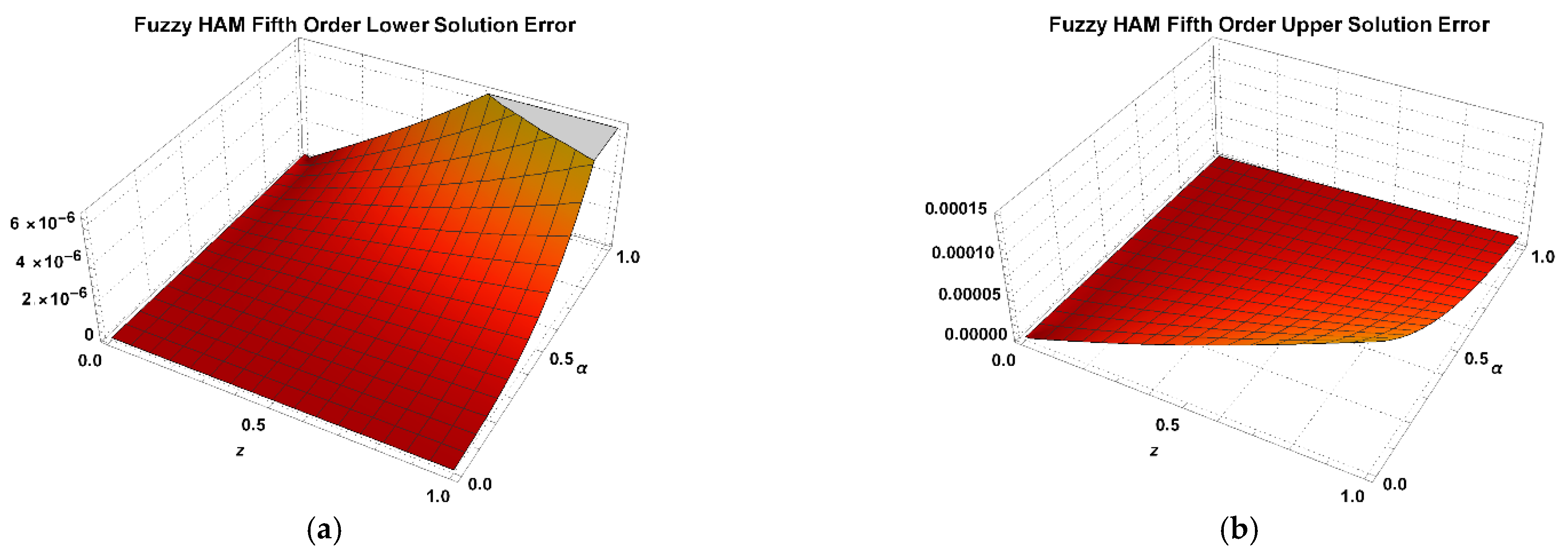
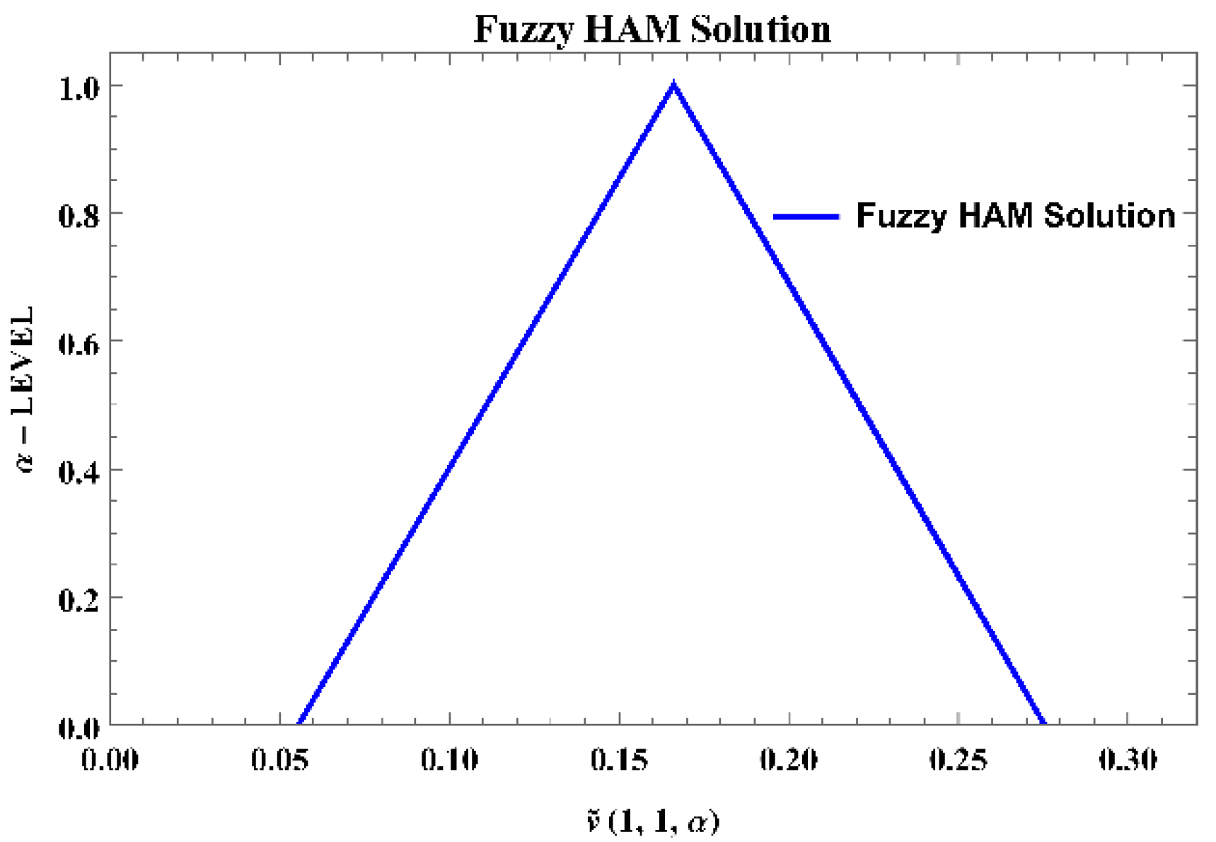
One can detect the valid region for the best values of $\tilde{\hslash }\left(\alpha \right)$ is $-1.2 \le \tilde{\hslash }\left(\alpha \right)\le -0.8$. The line segment of the fifth-order fuzzy HAM solution is nearly parallel to the horizontal axis on the region $-1.2 \le \tilde{\hslash }\left(\alpha \right)\le -0.8$ such that the optimal value is $\tilde{\hslash }\left(\alpha \right)=-0.9960451$ for all $\alpha \in \left[0, 1\right]$. Due to the fact that Equation (36) does not have an exact solution, we make use of the residual Formula (28) in order to determine the HAM solution of Equation (36) accurately. Hence, the solution is displayed in

Table 3. The 5th-order fuzzy approximate-analytical solution of Equation (36) and accuracy at $\tilde{\hslash }\left(\alpha \right)=-0.9960451$, $z=1$, $t=1$, for all $\alpha \in \left[0, 1\right]$.

$\mathit{\alpha }$	${\underset{¯}{\mathit{v}}}_{\mathit{H}\mathit{A}{\mathit{M}}_{\mathbf{5}}}$	${\overline{\mathit{v}}}_{\mathit{H}\mathit{A}{\mathit{M}}_{\mathbf{5}}}$	${\underset{¯}{\mathit{E}}}_{\mathit{H}\mathit{A}{\mathit{M}}_{\mathbf{5}}}$	${\overline{\mathit{E}}}_{\mathit{H}\mathit{A}{\mathit{M}}_{\mathbf{5}}}$
0	$0.0555368$	$0.275444$	$4.753646\times {10}^{-8}$	$1.468953\times {10}^{-4}$
0.2	$0.0777263$	$0.253736$	$2.708646\times {10}^{-7}$	$9.888449\times {10}^{-5}$
0.4	$0.0998906$	$0.231948$	$9.690159\times {10}^{-7}$	$6.392799\times {10}^{-5}$
0.6	$0.122022$	$0.210084$	$2.653378\times {10}^{-6}$	$3.939058\times {10}^{-5}$
0.8	$0.144115$	$0.188153$	$6.0984\times {10}^{-6}$	$2.289732\times {10}^{-5}$
1	$0.166161$	$0.166161$	$1.237929\times {10}^{-5}$	$1.237929\times {10}^{-5}$

and

Table 4. The 5th-order fuzzy approximate-analytical solution of Equation (36) and accuracy at $\tilde{\hslash }\left(\alpha \right)=-1$, $z=1$, $t=1$, for all $\alpha \in \left[0, 1\right]$.

$\mathit{\alpha }$	${\underset{¯}{\mathit{v}}}_{\mathit{H}\mathit{A}{\mathit{M}}_{\mathbf{5}}}$	${\overline{\mathit{v}}}_{\mathit{H}\mathit{A}{\mathit{M}}_{\mathbf{5}}}$	${\underset{¯}{\mathit{E}}}_{\mathit{H}\mathit{A}{\mathit{M}}_{\mathbf{5}}}$	${\overline{\mathit{E}}}_{\mathit{H}\mathit{A}{\mathit{M}}_{\mathbf{5}}}$
0	$0.0555368$	$0.275444$	$4.101186\times {10}^{-8}$	$1.073353\times {10}^{-4}$
0.2	$0.0777263$	$0.253737$	$2.191314\times {10}^{-7}$	$7.293031\times {10}^{-5}$
0.4	$0.0998906$	$0.231948$	$7.631432\times {10}^{-7}$	$4.755128\times {10}^{-5}$
0.6	$0.122022$	$0.210084$	$2.058428\times {10}^{-6}$	$2.953253\times {10}^{-5}$
0.8	$0.144115$	$0.188153$	$4.682052\times {10}^{-6}$	$1.729806\times {10}^{-5}$
1	$0.166161$	$0.166161$	$9.424361\times {10}^{-6}$	$9.424361\times {10}^{-6}$

with two different values of $\tilde{\hslash }\left(\alpha \right)$, and Figure 5 and Figure 6 show the accuracy and compliance with the fuzzy triangular number, as follows:

Meanwhile, the lower and upper solution are demonstrated in Figure 6 as shown below, taking the triangle shape to comply with the fuzzy theory.

The findings presented in Table 3 and Table 4 as well as Figure 6 demonstrate that the 5th-order HAM is capable of satisfying the triangular solution of the fuzzy differential equations for Equation (36), and it is able to do so with a respectable degree of accuracy given the absence of an exact solution.

7.3. Linear FRDE

Let us consider the following linear reaction–diffusion equation,

$$\begin{array}{ll}\frac{\partial }{\partial t}\tilde{v}\left(z,t\right)=\frac{{\partial }^2}{\partial z^2}\tilde{v}\left(z,t\right)+\tilde{v}\left(z,t\right)& 0<z<0.4,0<t<0.6\\ \tilde{v}\left(z,0\right)={\tilde{\gamma }}_3{z}^3& \end{array}$$

(39)

Applying the analysis described in Section 5, we will have a lower and upper defuzzified model for $0<z<0.4$, $0<t<0.6$, and all $\alpha \in \left[0, 1\right]$ as,

$$\begin{array}{l}\frac{\partial }{\partial t}\underset{\_}{v}\left(z,t;\alpha \right)-\frac{{\partial }^2}{\partial z^2}\underset{\_}{v}\left(z,t;\alpha \right)-\underset{\_}{v}\left(z,t;\alpha \right)=0\\ \underset{\_}{v}\left(z,0;\alpha \right)=\left(\alpha -1\right)z^3\end{array}$$

(40a)

$$\begin{array}{l}\frac{\partial }{\partial t}\overline{v}\left(z,t;\alpha \right)-\frac{{\partial }^2}{\partial z^2}\overline{v}\left(z,t;\alpha \right)-\overline{v}\left(z,t;\alpha \right)=0\\ \overline{v}\left(z,0;\alpha \right)=\left(1-\alpha \right)z^3\end{array}$$

(40b)

with the exact solution

$$\underset{\_}{v}\left(z,t;\alpha \right)=\left(\alpha -1\right)\left(z^2+6t\right)z{e}^t$$

$$\overline{v}\left(z,t;\alpha \right)=\left(1-\alpha \right)\left(z^2+6t\right)z{e}^t$$

Thus, using Equations (40a) and (40b) leads to the following linear, nonlinear operator, and the initial approximation for the lower and upper problem,

$$\mathcal{L}\left[\underset{\_}{v}\left(z,t;\alpha \right)\right]=\frac{\partial }{\partial t}\underset{\_}{v}\left(z,t;\alpha \right)$$

$$\mathcal{N}\left[\underset{\_}{v}\left(z,t;\alpha \right)\right]=\frac{\partial }{\partial t}\underset{\_}{v}\left(z,t;\alpha \right)-\frac{{\partial }^2}{\partial z^2}\underset{\_}{v}\left(z,t;\alpha \right)-\underset{\_}{v}\left(z,t;\alpha \right)$$

$${\underset{\_}{\nu }}_0\left(z,0;\alpha \right)=\left(\alpha -1\right)z^3$$

also, the following for the upper problem,

$$\mathcal{L}\left[\overline{v}\left(z,t;\alpha \right)\right]=\frac{\partial }{\partial t}\overline{v}\left(z,t;\alpha \right)$$

$$\mathcal{N}\left[\overline{v}\left(z,t;\alpha \right)\right]=\frac{\partial }{\partial t}\overline{v}\left(z,t;\alpha \right)-\frac{{\partial }^2}{\partial z^2}\overline{v}\left(z,t;\alpha \right)-\overline{v}\left(z,t;\alpha \right)$$

$${\overline{\nu }}_0\left(z,0;\alpha \right)=\left(1-\alpha \right)z^3$$

Furthermore, the lower and upper mth-order solution for $m\ge 1$ is,

$$\begin{array}{l}{\underset{\_}{\nu }}_m\left(z,t;\alpha \right)={\chi }_m{\underset{\_}{\nu }}_{m-1}\left(z,t;\alpha \right)+\underset{\_}{\hslash }\left(\alpha \right){\mathcal{L}}^{-1}\left[{\mathcal{R}}_m\left[{\overrightarrow{\underset{\_}{\nu }}}_{m-1}\left(z,t;\alpha \right)\right]\right]\\ ={\chi }_m{\underset{\_}{\nu }}_{m-1}\left(z,t;\alpha \right)+\underset{\_}{\hslash }\left(\alpha \right){{\displaystyle \int }}_0^t{\mathcal{R}}_m\left[{\overrightarrow{\underset{\_}{\nu }}}_{m-1}\left(z,t;\alpha \right)\right]d\tau \end{array}$$

(41a)

Subject to ${\underset{\_}{\nu }}_m\left(z,0;\alpha \right)=\left(\alpha -1\right)z^3$, where

$$\begin{array}{l}{\mathcal{R}}_m\left[{\overrightarrow{\underset{\_}{\nu }}}_{m-1}\left(z,t;\alpha \right)\right]\\ =\frac{\partial }{\partial t}{\underset{\_}{\nu }}_{m-1}\left(z,t;\alpha \right)-\frac{{\partial }^2}{\partial z^2}{\underset{\_}{\nu }}_{m-1}\left(z,t;\alpha \right)-{\underset{\_}{\nu }}_{m-1}\left(z,t;\alpha \right)\end{array}$$

$$\begin{array}{l}{\overline{\nu }}_m\left(z,t;\alpha \right)={\chi }_m{\overline{\nu }}_{m-1}\left(z,t;\alpha \right)+\overline{\hslash }\left(\alpha \right){\mathcal{L}}^{-1}\left[{\mathcal{R}}_m\left[{\overrightarrow{\overline{v}}}_{m-1}\left(z,t;\alpha \right)\right]\right]\\ ={\chi }_m{\overline{\nu }}_{m-1}\left(z,t;\alpha \right)+\overline{\hslash }\left(\alpha \right){{\displaystyle \int }}_0^t{\mathcal{R}}_m\left[{\overrightarrow{\overline{v}}}_{m-1}\left(z,t;\alpha \right)\right]d\tau \end{array}$$

(41b)

Subject to ${\overline{v}}_m\left(z,0;\alpha \right)=\left(1-\alpha \right)z^3$, where

$$\begin{array}{l}{\mathcal{R}}_m\left[{\overrightarrow{\overline{v}}}_{m-1}\left(z,t;\alpha \right)\right]\\ =\frac{\partial }{\partial t}{\overline{\nu }}_{m-1}\left(z,t;\alpha \right)-\frac{{\partial }^2}{\partial z^2}{\overline{\nu }}_{m-1}\left(z,t;\alpha \right)-{\overline{\nu }}_{m-1}\left(z,t;\alpha \right)\end{array}$$

Hence, the 10th-order fuzzy solution obtained as ${\tilde{v}}_{10}\left(z,t;h;\alpha \right)$ will depend on the values of $\tilde{\hslash }\left(\alpha \right)$ at all values of $\alpha \in \left[0, 1\right]$. Acceding to Ref. [44], the valid region of $\tilde{\hslash }\left(\alpha \right)$ is a horizontal line segment, and referring to the illustrative Figure 7 below, one can detect that the valid region for the best values of $\tilde{\hslash }\left(\alpha \right)$ is $-1.5 \le \tilde{\hslash }\left(\alpha \right)\le -0.7$.

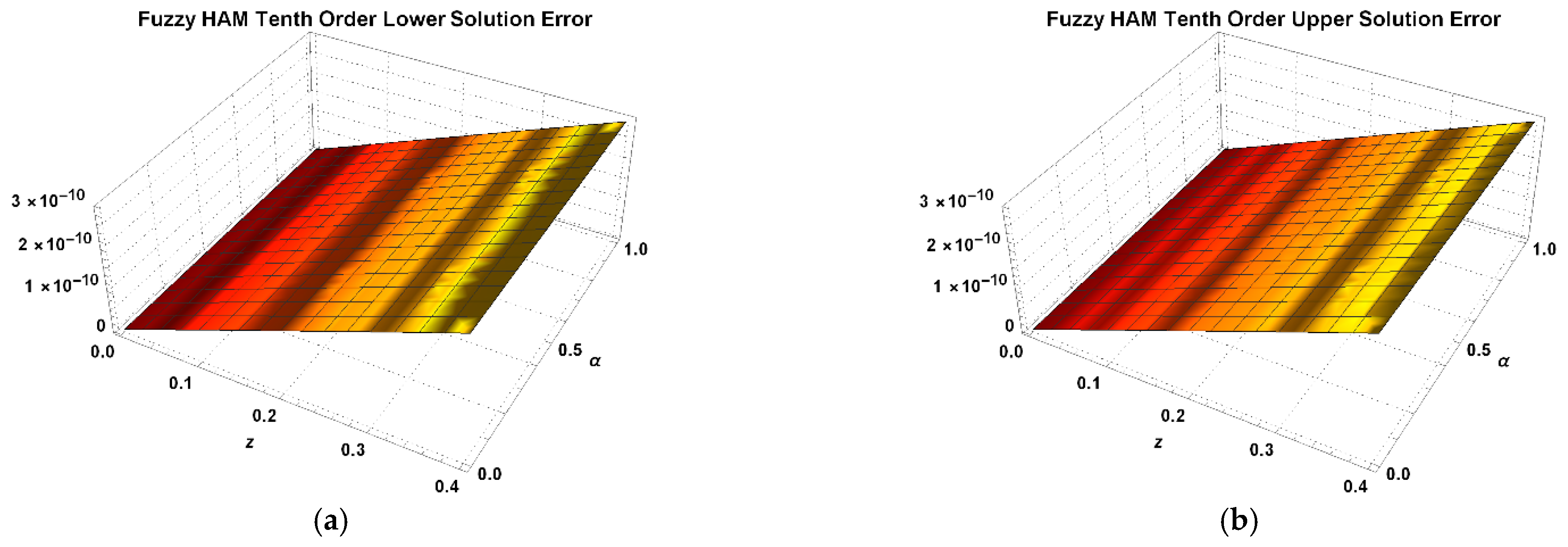
The line segment of the fuzzy HAM solution is nearly parallel to the horizontal axis on the region $-1.5 \le \tilde{\hslash }\left(\alpha \right)\le -0.7$ such that the optimal value is $\tilde{\hslash }\left(\alpha \right)=-1.1131254$ for all $\alpha \in \left[0, 1\right]$. Hence, the solution is displayed in

Table 5. The 10th-order fuzzy approximate-analytical solution of Equation (39) and accuracy at $\tilde{\hslash }\left(\alpha \right)=-1.1131254$, $z=0.4$, $t=0.6$, for all $\alpha \in \left[0, 1\right]$.

$\mathit{\alpha }$	${\underset{¯}{\mathit{v}}}_{\mathit{H}\mathit{A}{\mathit{M}}_{\mathbf{10}}}$	${\overline{\mathit{v}}}_{\mathit{H}\mathit{A}{\mathit{M}}_{\mathbf{10}}}$	${\underset{¯}{\mathit{E}}}_{\mathit{H}\mathit{A}{\mathit{M}}_{\mathbf{10}}}$	${\overline{\mathit{E}}}_{\mathit{H}\mathit{A}{\mathit{M}}_{\mathbf{10}}}$
0	−2.740467	2.740467	$7.351959\times {10}^{-10}$	$7.351959\times {10}^{-10}$
0.2	−2.192373	2.192373	$5.88138\times {10}^{-10}$	$5.88138\times {10}^{-10}$
0.4	−1.64428	1.64428	$4.410798\times {10}^{-10}$	$4.410798\times {10}^{-10}$
0.6	−1.096187	1.096187	$2.937726\times {10}^{-10}$	$2.937726\times {10}^{-10}$
0.8	−0.5480933	0.5480933	$1.469642\times {10}^{-10}$	$1.469642\times {10}^{-10}$
1	$1.421\times {10}^{-14}$	$-1.421\times {10}^{-14}$	$1.421085\times {10}^{-14}$	$1.421085\times {10}^{-14}$

and

Table 6. The 10th-order fuzzy approximate-analytical solution of Equation (39) and accuracy at $\tilde{\hslash }\left(\alpha \right)=-1$, $z=0.4$, $t=0.6$, for all $\alpha \in \left[0, 1\right]$.

$\mathit{\alpha }$	${\underset{¯}{\mathit{v}}}_{\mathit{H}\mathit{A}{\mathit{M}}_{\mathbf{10}}}$	${\overline{\mathit{v}}}_{\mathit{H}\mathit{A}{\mathit{M}}_{\mathbf{10}}}$	${\underset{¯}{\mathit{E}}}_{\mathit{H}\mathit{A}{\mathit{M}}_{\mathbf{10}}}$	${\overline{\mathit{E}}}_{\mathit{H}\mathit{A}{\mathit{M}}_{\mathbf{10}}}$
0	−2.740467	2.740467	$2.543519\times {10}^{-9}$	$2.543519\times {10}^{-9}$
0.2	−2.192373	2.192373	$2.034885\times {10}^{-9}$	$2.034885\times {10}^{-9}$
0.4	−1.64428	1.64428	$1.526251\times {10}^{-9}$	$1.526251\times {10}^{-9}$
0.6	−1.096187	1.096187	$1.017506\times {10}^{-9}$	$1.017506\times {10}^{-9}$
0.8	−0.5480933	0.5480933	$5.089835\times {10}^{-10}$	$5.089835\times {10}^{-10}$
1	$2.300\times {10}^{-13}$	$-2.300\times {10}^{-13}$	$2.300382\times {10}^{-13}$	$2.300382\times {10}^{-13}$

with two different values of $\tilde{\hslash }\left(\alpha \right)$, and Figure 8 and Figure 9 show the accuracy and compliance with the fuzzy triangular number as follows.

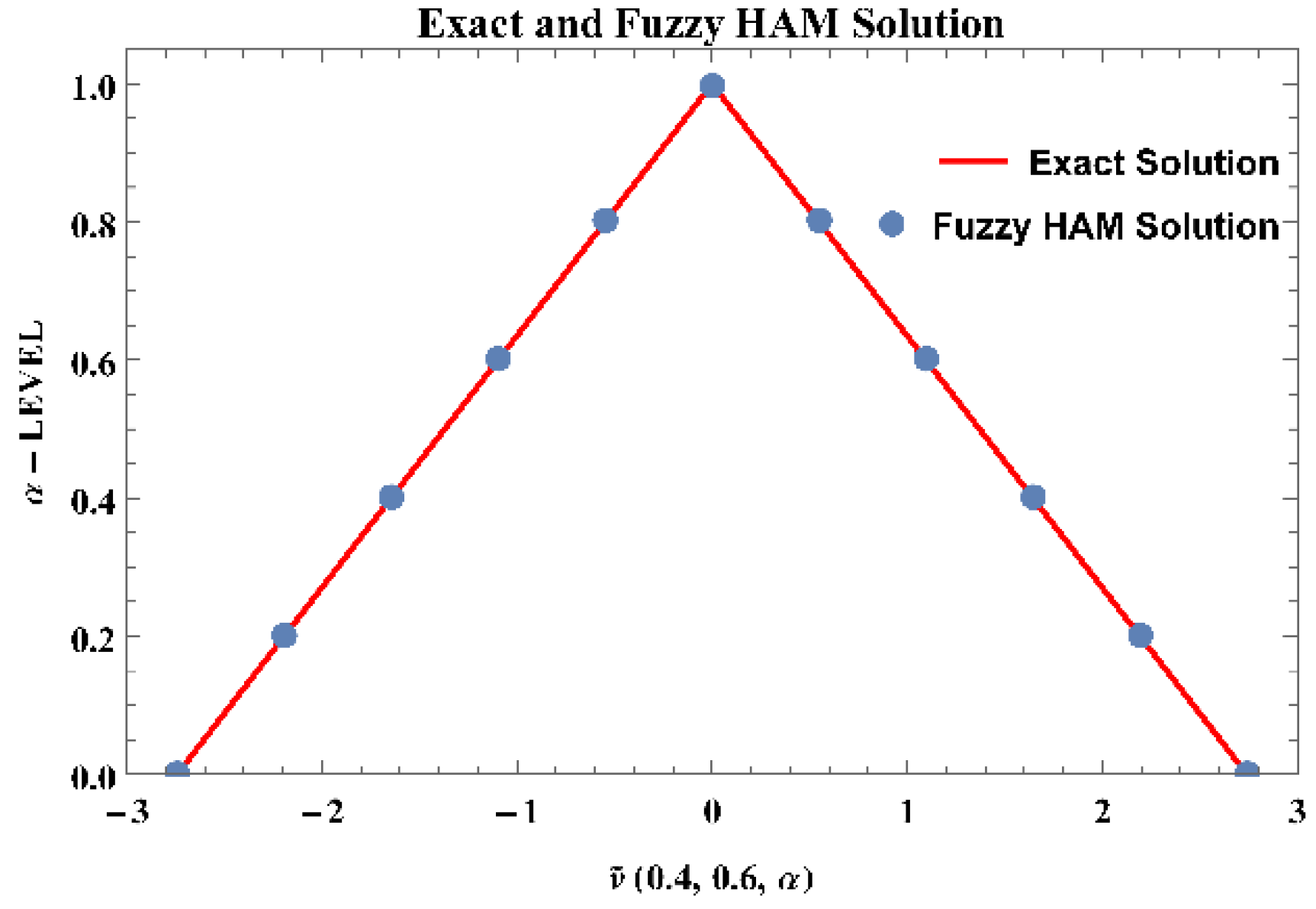
Meanwhile, the lower and upper solution are demonstrated in Figure 9 as shown below, taking the triangle shape to comply with the fuzzy theory.

The findings presented in Table 5 and Table 6 as well as Figure 9 indicate that the 10th-order HAM satisfies the triangular solution of the fuzzy differential equations for Equation (39), and it does so with a high degree of precision that is comparable to that of an exact solution. These findings were obtained by analyzing the data presented in the aforementioned tables.

7.4. Nonlinear FRDE

Let us consider the following fuzzy KPP equation,

$$\begin{array}{ll}\frac{\partial }{\partial t}\tilde{v}\left(z,t\right)=\frac{{\partial }^2}{\partial z^2}\tilde{v}\left(z,t\right)+\tilde{v}\left(z,t\right)\left[1-\tilde{v}\left(z,t\right)\right]& 0<z<0.2,0<t<0.2\\ \tilde{v}\left(z,0\right)={\tilde{\gamma }}_3{z}^2& \end{array}$$

(42)

Applying the analysis described in Section 4, we will have a lower, and upper defuzzified model for $0<z<0.2$, $0<t<0.2$, and all $\alpha \in \left[0, 1\right]$ as,

$$\begin{array}{l}\frac{\partial }{\partial t}\underset{\_}{v}\left(z,t;\alpha \right)-\frac{{\partial }^2}{\partial z^2}\underset{\_}{v}\left(z,t;\alpha \right)-\underset{\_}{v}\left(z,t;\alpha \right)\left[1-\underset{\_}{v}\left(z,t;\alpha \right)\right]=0\\ \underset{\_}{v}\left(z,0;\alpha \right)=\left(0.1+0.4\alpha \right)z^2\end{array}$$

(43a)

$$\begin{array}{l}\frac{\partial }{\partial t}\overline{v}\left(z,t;\alpha \right)-\frac{{\partial }^2}{\partial z^2}\overline{v}\left(z,t;\alpha \right)-\overline{v}\left(z,t;\alpha \right)\left[1-\overline{v}\left(z,t;\alpha \right)\right]=0\\ \overline{v}\left(z,0;\alpha \right)=\left(0.9-0.4\alpha \right)z^2\end{array}$$

(43b)

Thus, using Equations (43a) and (43b) leads to the following linear, nonlinear operator, and the initial approximation for the lower and upper problem,

$$\mathcal{L}\left[\underset{\_}{v}\left(z,t;\alpha \right)\right]=\frac{\partial }{\partial t}\underset{\_}{v}\left(z,t;\alpha \right)$$

$$\mathcal{N}\left[\underset{\_}{v}\left(z,t;\alpha \right)\right]=\frac{\partial }{\partial t}\underset{\_}{v}\left(z,t;\alpha \right)-\frac{{\partial }^2}{\partial z^2}\underset{\_}{v}\left(z,t;\alpha \right)-\underset{\_}{v}\left(z,t;\alpha \right)\left[1-\underset{\_}{v}\left(z,t;\alpha \right)\right]$$

$${\underset{\_}{\nu }}_0\left(z,0;\alpha \right)=\left(0.1+0.4\alpha \right)z^2$$

also, the following for the upper problem,

$$\mathcal{L}\left[\overline{v}\left(z,t;\alpha \right)\right]=\frac{\partial }{\partial t}\overline{v}\left(z,t;\alpha \right)$$

$$\mathcal{N}\left[\overline{v}\left(z,t;\alpha \right)\right]=\frac{\partial }{\partial t}\overline{v}\left(z,t;\alpha \right)-\frac{{\partial }^2}{\partial z^2}\overline{v}\left(z,t;\alpha \right)-\overline{v}\left(z,t;\alpha \right)\left[1-\overline{v}\left(z,t;\alpha \right)\right]$$

$${\overline{\nu }}_0\left(z,0;\alpha \right)=\left(0.9-0.4\alpha \right)z^2$$

Furthermore, the lower and upper mth-order solution for $m\ge 1$ is

$$\begin{array}{l}{\underset{\_}{\nu }}_m\left(z,t;\alpha \right)={\chi }_m{\underset{\_}{\nu }}_{m-1}\left(z,t;\alpha \right)+\underset{\_}{\hslash }\left(\alpha \right){\mathcal{L}}^{-1}\left[{\mathcal{R}}_m\left[{\overrightarrow{\underset{\_}{\nu }}}_{m-1}\left(z,t;\alpha \right)\right]\right]\\ ={\chi }_m{\underset{\_}{\nu }}_{m-1}\left(z,t;\alpha \right)+\underset{\_}{\hslash }\left(\alpha \right){{\displaystyle \int }}_0^t{\mathcal{R}}_m\left[{\overrightarrow{\underset{\_}{\nu }}}_{m-1}\left(z,t;\alpha \right)\right]d\tau \end{array}$$

(44a)

Subject to ${\underset{\_}{\nu }}_m\left(z,0;\alpha \right)=\left(0.1+0.4\alpha \right)z^2$, where

$$\begin{array}{l}{\mathcal{R}}_m\left[{\overrightarrow{\underset{\_}{\nu }}}_{m-1}\left(z,t;\alpha \right)\right]\\ =\frac{\partial }{\partial t}{\underset{\_}{\nu }}_{m-1}\left(z,t;\alpha \right)-\frac{{\partial }^2}{\partial z^2}{\underset{\_}{\nu }}_{m-1}\left(z,t;\alpha \right)-{\underset{\_}{\nu }}_{m-1}\left(z,t;\alpha \right)\left[1-{\underset{\_}{\nu }}_{m-1}\left(z,t;\alpha \right)\right]\end{array}$$

$$\begin{array}{l}{\overline{\nu }}_m\left(z,t;\alpha \right)={\chi }_m{\overline{\nu }}_{m-1}\left(z,t;\alpha \right)+\overline{\hslash }\left(\alpha \right){\mathcal{L}}^{-1}\left[{\mathcal{R}}_m\left[{\overrightarrow{\overline{v}}}_{m-1}\left(z,t;\alpha \right)\right]\right]\\ ={\chi }_m{\overline{\nu }}_{m-1}\left(z,t;\alpha \right)+\overline{\hslash }\left(\alpha \right){{\displaystyle \int }}_0^t{\mathcal{R}}_m\left[{\overrightarrow{\overline{v}}}_{m-1}\left(z,t;\alpha \right)\right]d\tau \end{array}$$

(44b)

Subject to ${\overline{v}}_m\left(z,0;\alpha \right)=\left(0.9-0.4\alpha \right)z^2$, where

$$\begin{array}{l}{\mathcal{R}}_m\left[{\overrightarrow{\overline{v}}}_{m-1}\left(z,t;\alpha \right)\right]\\ =\frac{\partial }{\partial t}{\overline{\nu }}_{m-1}\left(z,t;\alpha \right)-\frac{{\partial }^2}{\partial z^2}{\overline{\nu }}_{m-1}\left(z,t;\alpha \right)-{\overline{\nu }}_{m-1}\left(z,t;\alpha \right)\left[1-{\overline{\nu }}_{m-1}\left(z,t;\alpha \right)\right]\end{array}$$

Hence, a 5th-order fuzzy solution obtained as ${\tilde{v}}_5\left(z,t;h;\alpha \right)$ will depend on the values of $\tilde{\hslash }\left(\alpha \right)$ at all values of $\alpha \in \left[0, 1\right]$. According to [44], the valid region of $\tilde{\hslash }\left(\alpha \right)$ is a horizontal line segment, and referring to the illustrative Figure 10 below, one can detect the valid region for the best values of $\tilde{\hslash }\left(\alpha \right)$ is $-1.2 \le \tilde{\hslash }\left(\alpha \right)\le -0.7$.

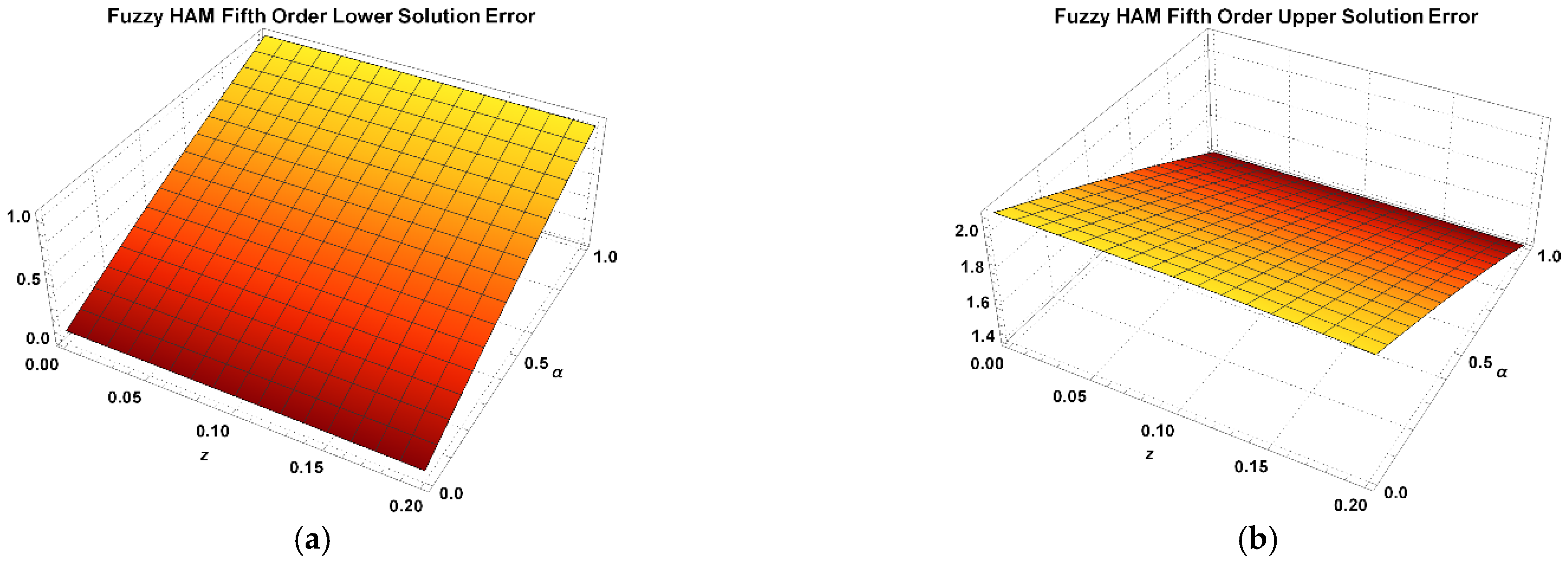
The line segment of the fuzzy HAM solution is nearly parallel to the horizontal axis on the region $-1.2 \le \tilde{\hslash }\left(\alpha \right)\le -0.7$ such that the optimal value is $\tilde{\hslash }\left(\alpha \right)=-1.0705826$ for all $\alpha \in \left[0, 1\right]$. Here, Equation (36) does not have an exact solution; we make use of the residual Formula (28) as in Example 4.2 in order to determine the HAM solution of Equation (42) accurately. Hence, the solution is displayed in

Table 7. The 5th-order fuzzy approximate-analytical solution of Equation (42) and accuracy at $\tilde{\hslash }\left(\alpha \right)=-1.0705826$, $z=0.2$, $t=0.2$, for all $\alpha \in \left[0, 1\right]$.

$\mathit{\alpha }$	${\underset{\_}{\mathit{v}}}_{\mathit{H}\mathit{A}{\mathit{M}}_{\mathbf{5}}}$	${\overline{\mathit{v}}}_{\mathit{H}\mathit{A}{\mathit{M}}_{\mathbf{5}}}$	${\underset{\_}{\mathit{E}}}_{\mathit{H}\mathit{A}{\mathit{M}}_{\mathbf{5}}}$	${\overline{\mathit{E}}}_{\mathit{H}\mathit{A}{\mathit{M}}_{\mathbf{5}}}$
0	0.0528799	0.426346	$3.188222\times {10}^{-5}$	$2.512498\times {10}^{-2}$
0.2	0.0939929	0.392061	$1.246993\times {10}^{-4}$	$1.587041\times {10}^{-2}$
0.4	0.134112	0.357252	$2.427401\times {10}^{-4}$	$9.33875\times {10}^{-3}$
0.6	0.173295	0.32186	$2.787076\times {10}^{-4}$	$4.957079\times {10}^{-3}$
0.8	0.211603	0.285827	$5.568322\times {10}^{-5}$	$2.216259\times {10}^{-3}$
1	0.249094	0.249094	$6.71717\times {10}^{-4}$	$6.71717\times {10}^{-4}$

and

Table 8. The 5th-order fuzzy approximate-analytical solution of Equation (42) and accuracy at $\tilde{\hslash }\left(\alpha \right)=-1$, $z=0.2$, $t=0.2$, for all $\alpha \in \left[0, 1\right]$.

$\mathit{\alpha }$	${\underset{¯}{\mathit{v}}}_{\mathit{H}\mathit{A}{\mathit{M}}_{\mathbf{5}}}$	${\overline{\mathit{v}}}_{\mathit{H}\mathit{A}{\mathit{M}}_{\mathbf{5}}}$	${\underset{¯}{\mathit{E}}}_{\mathit{H}\mathit{A}{\mathit{M}}_{\mathbf{5}}}$	${\overline{\mathit{E}}}_{\mathit{H}\mathit{A}{\mathit{M}}_{\mathbf{5}}}$
0	0.0528779	0.423486	$4.22758\times {10}^{-5}$	$4.107174\times {10}^{-2}$
0.2	0.0939758	0.38991	$3.860324\times {10}^{-4}$	$3.301468\times {10}^{-2}$
0.4	0.134053	0.355682	$1.282258\times {10}^{-3}$	$2.564467\times {10}^{-2}$
0.6	0.173157	0.320757	$2.928706\times {10}^{-3}$	$1.912003\times {10}^{-2}$
0.8	0.211333	0.285087	$5.469668\times {10}^{-3}$	$1.355058\times {10}^{-2}$
1	0.248628	0.248628	$8.996911\times {10}^{-3}$	$8.996911\times {10}^{-3}$

with two different values of $\tilde{\hslash }\left(\alpha \right)$, and Figure 11 and Figure 12 show the accuracy and compliance with the fuzzy triangular number as follows.

Meanwhile, the lower and upper solution are demonstrated in Figure 12 as shown below, taking the triangle shape to comply with the fuzzy theory,

Figure 12. The approximate lower and upper solution of Equation (43) at $\tilde{\hslash }\left(\alpha \right)=-1.0705826$, $z=0.2$, $t=0.2$, for all $\alpha \in \left[0, 1\right]$.

Figure 12. The approximate lower and upper solution of Equation (43) at $\tilde{\hslash }\left(\alpha \right)=-1.0705826$, $z=0.2$, $t=0.2$, for all $\alpha \in \left[0, 1\right]$.

The conclusions that are presented in Table 7 and Table 8, in addition to Figure 6, illustrate that the 5th-order HAM satisfies the triangular solution of the fuzzy differential equations for Equation (42), and that it is able to do that with a good degree of accuracy despite there not being an exact solution. This is proven by the fact that the 5th-order HAM can be seen in Figure 11 and Figure 12.

8. Conclusions

This work aims to extend HAM to a new form to solve approximately fuzzy partial differential equations. The HAM has the potential to provide a particular technique for guaranteeing a convergence solution in series form. In this paper, the concepts of fuzzy set theory are considered to be associated with the sense of fuzzy derivatives properties for a new general form of HAM. This form was presented and extended to new forms for the approximate solution of fuzzy heat and wave equations, which was then followed by a full fuzzy analysis.

Under the new forms of HAM, the effectiveness of this convergence analysis is demonstrated through the use of both mathematical and graphical illustrations.

The scheme was tested through four examples involving linear, nonlinear, homogeneous, and nonhomogeneous FPDEs, which were followed by complete fuzzy analysis demonstrating the method’s capability. The results showed that the presented problems possessed an approximate convergent solution for the best values of convenience control perimeters of HAM to satisfy properties of fuzzy numbers. So, using HAM instead of conventional approximate-analytical approaches is highly recommended because HAM converges faster to the solution and is more abridged. In addition, the accuracy of the nonlinear problems can be obtained through our method without the need for an exact solution, which is a distinct advantage of our approach.

Furthermore, the different orders of solutions applied to FRDEs and FWEs in this study confirm that this new extension of HAM is a feasible and capable approach to solving further FPDEs problems in science and engineering.

References

1. Zadeh, L.A. Fuzzy sets. Inf. Control. 1965, 8, 338–353. [Google Scholar] [CrossRef] [Green Version]
2. Chang, S.L.; Zadeh, L.A. On fuzzy mapping and control. IEEE SMC-2 Trans. Syst. Man Cybern. 1972, 1, 30–34. [Google Scholar] [CrossRef]
3. Dubois, D.; Prade, H. Towards fuzzy differential calculus part 3: Differentiation. Fuzzy Sets Syst. 1982, 8, 225–233. [Google Scholar] [CrossRef]
4. Puri, M.; Ralescu, D. Differentials of fuzzy functions. J. Math. Anal. Appl. 1983, 91, 552–558. [Google Scholar] [CrossRef] [Green Version]
5. Seikkala, S. On the fuzzy initial value problem. Fuzzy Sets Syst. 1987, 24, 319–330. [Google Scholar] [CrossRef]
6. Kandel, A.; Byatt, W. Fuzzy differential equations. In Proceedings of the International Conference on Cybernetics and Society, Tokyo, Japan, 3–7 November 1978. [Google Scholar]
7. Kandel, A.; Byatt, W. Fuzzy processes. Fuzzy Sets Syst. 1980, 4, 117–152. [Google Scholar] [CrossRef]
8. Kaleva, O. Fuzzy differential equations. Fuzzy Sets Syst. 1987, 24, 301–317. [Google Scholar] [CrossRef]
9. Kaleva, O. The cauchy problem for fuzzy differential equations. Fuzzy Sets Syst. 1990, 35, 389–396. [Google Scholar] [CrossRef]
10. He, O.; Yia, W. On fuzzy differential equations. Fuzzy Sets Syst. 1989, 32, 321–325. [Google Scholar] [CrossRef]
11. Bede, B. A note on “two-point boundary value problems associated with non-linear fuzzy differential equations”. Fuzzy Sets Syst. 2006, 157, 986–989. [Google Scholar] [CrossRef]
12. Bede, B.; Rudas, I.J.; Bencsik, A.L. First order linear fuzzy differential equations under generalized differentiability. Inf. Sci. 2007, 177, 1648–1662. [Google Scholar] [CrossRef]
13. Bede, B.; Gal, S.G. Generalizations of the differentiability of fuzzy-number-valued functions with applications to fuzzy differential equations. Fuzzy Sets Syst. 2005, 151, 581–599. [Google Scholar] [CrossRef]
14. Hüllermeier, E. An Approach to Modelling and Simulation of Uncertain Dynamical Systems. Int. J. Uncertain. Fuzziness Knowl. Based Syst. 1997, 5, 117–137. [Google Scholar] [CrossRef] [Green Version]
15. Buckley, J.; Feuring, T. Fuzzy initial value problem for Nth-order linear differential equations. Fuzzy Sets Syst. 2001, 121, 247–255. [Google Scholar] [CrossRef]
16. Das, B.; Mahapatra, N.K.; Maiti, M. Initial-Valued First-Order Fuzzy Differential Equation in Bi-Level Inventory Model with Fuzzy Demand. Math. Model. Anal. 2008, 13, 493–512. [Google Scholar] [CrossRef]
17. Allahviranloo, T.; Abbasbandy, S.; Salahshour, S.; Hakimzadeh, A. A new method for solving fuzzy linear differential equations. Computing 2010, 92, 181–197. [Google Scholar] [CrossRef]
18. Mondal, S.P.; Roy, T.K. First Order Linear Homogeneous Fuzzy Ordinary Differential Equation Based on Lagrange Multiplier Method. J. Soft Comput. Appl. 2013, 2013, 1–17. [Google Scholar] [CrossRef] [Green Version]
19. Buckley, J.J.; Feuring, T. Introduction to fuzzy partial differential equations. Fuzzy Sets Syst. 1999, 105, 241–248. [Google Scholar] [CrossRef]
20. Allahviranloo, T. Difference Methods for Fuzzy Partial Differential Equations. Comput. Methods Appl. Math. 2002, 2, 233–242. [Google Scholar] [CrossRef]
21. Nemati, K.; Matinfar, M. An Implicit Method for Fuzzy Parabolic Partial Differential Equations. J. Nonlinear Sci. Appl. 2008, 1, 61–71. [Google Scholar] [CrossRef] [Green Version]
22. Farajzadeh, A. An Explicit Method for Solving Fuzzy Partial Differential Equation. Int. Math. Forum 2010, 2010, 358–367. [Google Scholar] [CrossRef] [Green Version]
23. Allahviranloo, T.; Abbasbandy, S.; Rouhparvar, H. The exact solutions of fuzzy wave-like equations with variable coefficients by a variational iteration method. Appl. Soft Comput. 2011, 11, 2186–2192. [Google Scholar] [CrossRef]
24. Jafelice, R.M.; Almeida, C.; Meyer, J.; Vasconcelos, H. Fuzzy parameters in a partial differential equation model for population dispersal of leaf-cutting ants. Nonlinear Anal. Real World Appl. 2011, 12, 3397–3412. [Google Scholar] [CrossRef]
25. Mikaeilvand, N.; Khakrangin, S. Solving fuzzy partial differential equations by fuzzy two-dimensional differential transform method. Neural Comput. Appl. 2012, 21, 307–312. [Google Scholar] [CrossRef]
26. Bertone, A.M.; Jafelice, R.M.; de Barros, L.C.; Bassanezi, R.C. On fuzzy solutions for partial differential equations. Fuzzy Sets Syst. 2013, 219, 68–80. [Google Scholar] [CrossRef]
27. Allahviranloo, T.; Gouyandeh, Z.; Armand, A.; Hasanoglu, A. On fuzzy solutions for heat equation based on generalized Hukuhara differentiability. Fuzzy Sets Syst. 2015, 265, 1–23. [Google Scholar] [CrossRef]
28. Pirzada, U.; Vakaskar, D. Solution of fuzzy heat equations using Adomian Decomposition method. Int. J. Adv. Appl. Andm. 2015, 3, 87–91. [Google Scholar]
29. Mirzaee, F.; Yari, M.K. A novel computing three-dimensional differential transform method for solving fuzzy partial differential equations. Ain Shams Eng. J. 2016, 7, 695–708. [Google Scholar] [CrossRef] [Green Version]
30. Bertone, A.M.; Jafelice, R.M.; de Barros, L.C.; Gomide, F. Granular approximation of solutions of partial differential equations with fuzzy parameter. Granul. Comput. 2017, 3, 1–7. [Google Scholar] [CrossRef]
31. Altaie, S.A.; Saaban, A.; Jameel, A.F. Series solution of fuzzy linear Cauchy reaction-diffusion equation by using homotopy perturbation method. In Proceedings of the 13th IMT-GT International Conference on Mathematics, Statistics and their Applications (ICMSA2017), Kedah, Malaysia, 4–7 December 2017. [Google Scholar]
32. Altaie, S.; Jameel, A.; Saaban, A. A single convergent control parameter optimal homotopy asymptotic method approximate-analytical solution of fuzzy heat equation. ASM Sci. J. 2019, 12, 42–47. [Google Scholar]
33. Alikhani, R.; Bahrami, F. Fuzzy partial differential equations under the cross product of fuzzy numbers. Inf. Sci. 2019, 494, 80–99. [Google Scholar] [CrossRef]
34. Alikhani, R.; Bahrami, F.; Parvizi, S. Differential calculus of fuzzy multi-variable functions and its applications to fuzzy partial differential equations. Fuzzy Sets Syst. 2019, 375, 100–120. [Google Scholar] [CrossRef]
35. Osman, M.; Gong, Z.; Mustafa, A.M. Comparison of fuzzy Adomian decomposition method with fuzzy VIM for solving fuzzy heat-like and wave-like equations with variable coefficients. Adv. Differ. Equ. 2020, 2020, 327. [Google Scholar] [CrossRef]
36. Allahviranloo, T.; Ghobadi, M.; Matinfar, M. A fuzzy solution of wave equation by FFS-transform. Numer. Methods Partial Differ. Equ. 2020, 2020, 1–16. [Google Scholar] [CrossRef]
37. Chermahini, S.R.; Asgari, M.S. Analytical fuzzy triangular solutions of the wave equation. Soft Comput. 2020, 25, 363–378. [Google Scholar] [CrossRef]
38. Osman, M.; Gong, Z.; Mustafa, A.M. A fuzzy solution of nonlinear partial differential equations. Open J. Math. Anal. 2021, 5, 51–63. [Google Scholar] [CrossRef]
39. Altaie, S.A.; Saaban, A.; Jameel, A.F. Approximate analytical modelling of fuzzy reaction-diffusion equation. Int. J. Comput. Sci. Math. 2021, 13, 136–155. [Google Scholar] [CrossRef]
40. Liao, S.J. The Proposed Homotopy Analysis Techniques for the Solution of Nonlinear Problems. Ph.D. Dissertation, Shanghai Jiao Tong University, Shangha, China, 1992. [Google Scholar]
41. Liao, S. An approximate solution technique not depending on small parameters: A special example. Int. J. Nonlinear Mech. 1995, 30, 371–380. [Google Scholar] [CrossRef]
42. Liao, S.-J. A kind of approximate solution technique which does not depend upon small parameters—II. An application in fluid mechanics. Int. J. Nonlinear Mech. 1997, 32, 815–822. [Google Scholar] [CrossRef]
43. Liao, S. An explicit analytic solution to the Thomas–Fermi equation. Appl. Math. Comput. 2003, 144, 495–506. [Google Scholar] [CrossRef]
44. Liao, S.; Sherif, S. Beyond Perturbation: Introduction to the Homotopy Analysis Method, 1st ed.; Chapman & Hall/CRC Press: Boca Raton, FL, USA, 2004. [Google Scholar]
45. Yang, Y.; Song, J. On the generalized eigenvalue problem of Rossby waves vertical velocity under the condition of zonal mean flow and topography. Appl. Math. Lett. 2021, 121, 107485. [Google Scholar] [CrossRef]
46. Engelbrecht, J. Wave equations in mechanics. Est. J. Eng. 2013, 19, 273–282. [Google Scholar] [CrossRef] [Green Version]
47. Robinson, E.; Clark, D. The wave equation. Lead. Edge 1987, 6, 14–17. [Google Scholar] [CrossRef]
48. Olver, P. Introduction to Partial Differential Equations, 1st ed.; Springer International Publishing: Cham, Switzerland, 2014; p. 635. [Google Scholar]
Figure 1. The h-Curve of 10th-order fuzzy approximate-analytical solution of Equation (33) at α = 1 , z = 0.1 , t = 0.1 . (a) Fuzzy HAM lower h-Curve. (b) Fuzzy HAM upper h-Curve.
Fractalfract 06 00419 g001
Figure 2. The accuracy of 10th-order fuzzy approximate-analytical solution of Equation (33) at ˜ α = 0.9852279 , t = 1 , 0 z 1 , for all α 0 ,   1 . (a) Fuzzy HAM lower error. (b) Fuzzy HAM upper error.
Fractalfract 06 00419 g002
Figure 3. The exact and approximate lower and upper solution of Equation (33) at ˜ α = 0.9852279 , z = 1 , t = 1 , for all α 0 ,   1 .
Fractalfract 06 00419 g003
Figure 4. The h-Curve of 5th-order fuzzy approximate-analytical solution of Equation (36) at α = 1 , z = 0.1 , t = 0.1 . (a) Fuzzy HAM lower h-Curve. (b) Fuzzy HAM upper h-Curve.
Fractalfract 06 00419 g004
Figure 5. The accuracy of the 5th-order fuzzy approximate-analytical solution of Equation (36) at ˜ α = 0.9960451 , t = 1 , 0 z 1 , for all α 0 ,   1 . (a) Fuzzy HAM lower error. (b) Fuzzy HAM upper error.
Fractalfract 06 00419 g005
Figure 6. The approximate lower and upper solution of Equation (36) at ˜ α = 0.9960451 , z = 1 , t = 1 , for all α 0 ,   1 .
Fractalfract 06 00419 g006
Figure 7. The h-Curve of 10th-order fuzzy approximate-analytical solution of Equation (39) at α = 1 , z = 0.4 , t = 0.6 . (a) Fuzzy HAM lower h-Curve. (b) Fuzzy HAM upper h-Curve.
Fractalfract 06 00419 g007
Figure 8. The accuracy of the 10th-order fuzzy approximate-analytical solution of Equation (39) at ˜ α = 1.1131254 , t = 0.6 , 0 z 0.4 , for all α 0 ,   1 . (a) Fuzzy HAM lower error. (b) Fuzzy HAM upper error.
Fractalfract 06 00419 g008
Figure 9. The approximate lower and upper solution of Equation (39) at ˜ α = 1.1131254 , z = 0.4 , t = 0.6 , for all α 0 ,   1 .
Fractalfract 06 00419 g009
Figure 10. The h-Curve of 5th-order fuzzy approximate-analytical solution of Equation (42) at α = 1 , z = 0.2 , t = 0.2 . (a) Fuzzy HAM lower h-Curve. (b) Fuzzy HAM upper h-Curve.
Fractalfract 06 00419 g010
Figure 11. The accuracy of 5th-order fuzzy approximate-analytical solution of Equation (42) at ˜ ( α ) = 1.0705826 , t = 0.2 , 0 z 0.2 , for all α [ 0 ,   1 ] . (a) Fuzzy HAM lower error. (b) Fuzzy HAM upper error.
Fractalfract 06 00419 g011