Article

A New Fractional Poisson Process Governed by a Recursive Fractional Differential Equation

Department of Financial and Actuarial Mathematics, Xi’an Jiaotong-Liverpool University, Suzhou 215123, China
Fractal Fract. 2022, 6(8), 418; https://doi.org/10.3390/fractalfract6080418
Submission received: 6 July 2022 / Revised: 25 July 2022 / Accepted: 27 July 2022 / Published: 29 July 2022
(This article belongs to the Special Issue Fractional Calculus Operators and the Mittag-Leffler Function)

Abstract

:
This paper proposes a new fractional Poisson process through a recursive fractional differential governing equation. Unlike the homogeneous Poison process, the Caputo derivative on the probability distribution of k jumps with respect to time is linked to all probability distribution functions of j jumps, where j is a non-negative integer less than or equal to k. The distribution functions of arrival times are derived, while the inter-arrival times are no longer independent and identically distributed. Further, this new fractional Poisson process can be interpreted as a homogeneous Poisson process whose natural time flow has been randomized, and the underlying time randomizing process has been studied. Finally, the conditional distribution of the kth order statistic from random number samples, counted by this fractional Poisson process, is also discussed.

1. Introduction

Since the inter-arrival times of a Poisson process being independent and exponentially distributed are not supported by real data (see [1,2] and references therein), the fractional Poisson processes have received various attention. There are several different approaches to this concept. Jumarie [3] studies the fractional version of the Poisson process through the fractional master equation. Laskin [4] modifies the differential equation governing the probability distribution function of a homogeneous Poisson process through the Riemann–Liouville fractional derivative.
Another approach, followed by [5] is to generalize the inter-arrival times of a homogeneous Poisson process through the Mittag–Leffler distribution (see [6]). Later, Reference [7] shows that this fractional version is a true renewal process, without the independent and stationary increments.
If we denote the homogeneous Poisson process as { N t } t 0 with intensity λ , where λ   >   0 , and β t β as the Caputo fractional derivative, where β     ( 0 ,   1 ) , i.e.,
β t β f ( t ) = 1 Γ ( 1 α ) 0 t ( t s ) α d d s f ( s ) d s ,
then one fractional method, proposed by [8] and denoted as { M t β } t 0 , is to generalize the probability distribution function of N t from
t P ( N t = k ) = λ P ( N t = k ) P ( N t = k 1 ) , k N 0 ,
to
β t β P ( M t β = k ) = λ P ( M t β = k ) P ( M t β = k 1 ) , k N 0 ,
i.e., it is the time being fictionalized from a calculus point of view. More interestingly, if we consider the inverse β -stable subordinator { E t β } t 0 , where β     ( 0 ,   1 ) , i.e.,
E [ e q E t β ] = E β ( q t β ) ,
where
E β ( z ) = j = 0 z j Γ ( β j + 1 ) , β C , ( β ) > 0
is the Mittag–Leffler function of one variable, and assume that { N t } t 0 and { E t β } t 0 are independent, then
M t β = d N E t β ,
i.e., it is the time being randomized from a probability point of view. Beghin and Orsingher [9], Meerschaert et al. [10] prove that { M t β } t 0 is still a renewal process with inter-arrival times being independent and identically Mittag–Leffler distributed random variables, and study the case where Equation (2) is generalized to the nth order differential equation. The probability distribution function of { M t β } t 0 is,
P M t β = k = λ t β k E β , β k + 1 k + 1 λ t β , k N 0 ,
where
E β , γ δ ( z ) = k = 0 ( δ ) k Γ ( β k + γ ) z k k ! , β , γ , δ C , ( β ) > 0
is the Mittag–Leffler function of three variables. Later, [11] describe the non-homogeneous version of this fractional Poisson process through its non-local governing equation. This fractional Poisson process has been applied in various fields. We refer to [12] for its applications in the transport of charged carriers, and [13] for its applications in risk theory.
Another type of fractional Poisson process, proposed by [14,15], is constructed through the integral representation, by replacing the Gaussian measure in the definition of fractional Brownian motion with the Poisson counting measure. This fractional version displays long range dependence, has a fatter tail than the Gaussian process, and converges to fractional Brownian motion in distribution. Wang et al. [16] study the non-homogeneous versions of this fractional process.
This paper defines a new fractional Poisson process, denoted as { N t β } t 0 , through a governing equation, which generalizes Equation (1) by connecting P ( N t β = k ) to P ( N t β = j ) for all j     k through Caputo fractional derivative, i.e.,
β t β P N t β = k = λ β j = 0 k ( β ) j j ! P N t β = k j , j , k N 0 .
Since P ( N t β   =   k )   =   0 for k     N 0 , then the upper bound of the summation on the right hand side can be extended to infinity. Thus, the fractional differentiation on the time of the probability distribution function is related to the probabilities of all possible values this new process could take. Particularly, when β   =   1 , the above equation goes back to Equation (1).
We first study the probability properties of this fractional Poisson process. Later, we find this fractional process can be interpreted as a homogeneous Poisson process whose natural time flow has been randomized, and the underlying time process at time one follows a Lamperti distribution. The transforms of this underlying time process have also been studied. Finally, we discuss the order statistics counted by this fractional Poisson process.

2. Main Results

Theorem 1. 
Let { N t β } t 0 be a fractional Poisson process with parameter λ   >   0 and β     ( 0 ,   1 ) , which satisfies the governing equation
β t β P N t β = k = λ β j = 0 k ( β ) j j ! P N t β = k j , j , k N 0 ,
where P ( N t β   =   k )   =   0 for k     N 0 . Then the probability distribution function of this process is
P N t β = k = ( 1 ) k k ! E β , 1 k λ β t β , k N 0 ,
where
E β , γ ( z ) = j = 0 z j Γ ( β j + γ ) , β , γ C , ( β ) > 0 ,
is the Mittag–Leffler function of two variables, and the probability density function of its arrival times { T k } k N is
f T k ( t ) = ( 1 ) k + 1 Γ ( k ) λ ( λ t ) β 1 E β , β + 1 k λ β t β , k N .
Proof. 
From the definition, we may write the right hand side of the governing equation into an infinite series,
β t β P N t β = k = λ β j = 0 ( β ) j j ! P N t β = k j ,
and therefore the Laplace transform of N t β is
β t β E e q N t β = λ β j = 0 ( β ) j j ! E e q N t β + j = λ β j = 0 ( β ) j j ! e q j E e q N t β = λ β 1 e q β E e q N t β .
Taking Laplace transform from t to s gives
s β L s E e q N t β s β 1 E e q N 0 β = λ β 1 e q β L s E e q N t β L s E e q N t β = s β 1 s β + λ β 1 e q β .
This leads to
E e q N t β = E β , 1 λ β 1 e q β t β = n = 0 λ β t β n Γ ( β n + 1 ) 1 e q β n = k = 0 e q k n = 0 λ β t β n Γ ( β n + 1 ) ( β n ) k k ! ,
and therefore
P N t β = k = 1 k ! n = 0 λ β t β n ( β n ) k Γ ( β n + 1 ) = 1 k ! n = 0 ( 1 ) k λ β t β n Γ ( β n + 1 k ) = ( 1 ) k k ! E β , 1 k λ β t β .
For the arrival times { T k } k N , since N t β k and T k t are equivalent, then we have
P T k t = j = k P N t β = j = j = k ( 1 ) j j ! E β , 1 j λ β t β = n = 0 λ β t β n Γ ( β n + 1 ) j = k 1 j ! Γ ( β n + j ) Γ ( β n ) = n = 0 λ β t β n Γ ( β n + 1 ) ( β n ) k k ! 2 F 1 ( 1 , k n β , 1 + k , 1 ) = n = 1 λ β t β n Γ ( β n + 1 ) ( β n ) k k ! Γ ( 1 + k ) Γ ( β n ) Γ ( k ) Γ ( 1 + β n ) = ( 1 ) k Γ ( k ) n = 1 λ β t β n Γ ( β n + 1 k ) 1 β n ,
where 2 F 1 ( α , β , γ , z ) is the Hypergeometric function; see [17] (Chapter 9). The proof is completed after differentiating it with respect to t once. □
Remark 1. 
1.
When β = 1 ,
E e q N t β = n = 0 λ 1 e q t n Γ ( n + 1 ) = exp λ t e q 1 P N t β = k = 1 k ! n = 0 ( 1 ) k ( λ t ) n Γ ( n + 1 k ) = 1 k ! n = k ( 1 ) k λ β t β n Γ ( n + 1 k ) = ( λ t ) k k ! e λ t ,
which goes back to a homogeneous Poisson process.
2.
Since β     ( 0 ,   1 ) , the integral representation of the Mittag–Leffler function remains [18] (Lemma 2.2.2), and we have
P N t β = k = ( 1 ) k k ! 1 2 π i c i c + i Γ ( s ) Γ ( 1 s ) Γ ( 1 k β s ) λ β t β s d s = ( 1 ) k k ! H 1 , 2 1 , 1 λ β t β | ( 0 , 1 ) ( 0 , 1 ) ( k , β ) ,
where H p , q m , n z | a i , A i 1 , p b j , B j 1 , q is the Fox’s H function. The convergence of this contour integral can be checked by [19] (Equation (1.13)) The integral representation, by closing the contour in two different directions, leads to
E β , γ ( z ) = j = 0 z j Γ ( β j + γ ) = j = 1 z j Γ ( γ β j ) ,
which determines the asymptotic behavior of these probability functions.
3.
Equation (8) indicates that
E e q N t 1 + t 2 β = E β , 1 λ β 1 e q β t 1 + t 2 β E β , 1 λ β 1 e q β t 1 β E β , 1 λ β 1 e q β t 2 β = E e q N t 1 β E e q N t 2 β ,
i.e., { N t β } t 0 no longer possesses independent increments and therefore loses the lack of memory property of the homogeneous Poisson process.
4.
Since
d d q E e q N t β = e q 1 e q β 1 t β λ β E β , β λ β 1 e q β t β ,
which tends to ∞ as q tends to 0, then E N t β n does not exist for all n N , unlike E M t β n .
Given Equation (6), Equation (5) can be verified directly.
β t β P N t β = k = 1 k ! n = 1 ( 1 ) k λ β n Γ ( β n + 1 k ) Γ ( β n + 1 ) Γ ( β n β + 1 ) t β ( n 1 ) = λ β 1 k ! n = 0 λ β n Γ ( β n + 1 ) ( β n β ) k t β n = λ β 1 k ! n = 0 λ β n Γ ( β n + 1 ) j = 0 k k j ( β ) j ( β n ) k j t β n = λ β j = 0 k k ! j ! ( k j ) ! ( β ) j 1 k ! n = 0 λ β n Γ ( β n + 1 ) ( 1 ) k j Γ ( β n + 1 ) Γ ( β n + 1 ( k j ) ) t β n = λ β j = 0 k ( β ) j j ! 1 ( k j ) ! n = 0 ( 1 ) k j λ β n Γ ( β n + 1 ( k j ) ) t β n = λ β j = 0 k ( β ) j j ! P N t β = k .
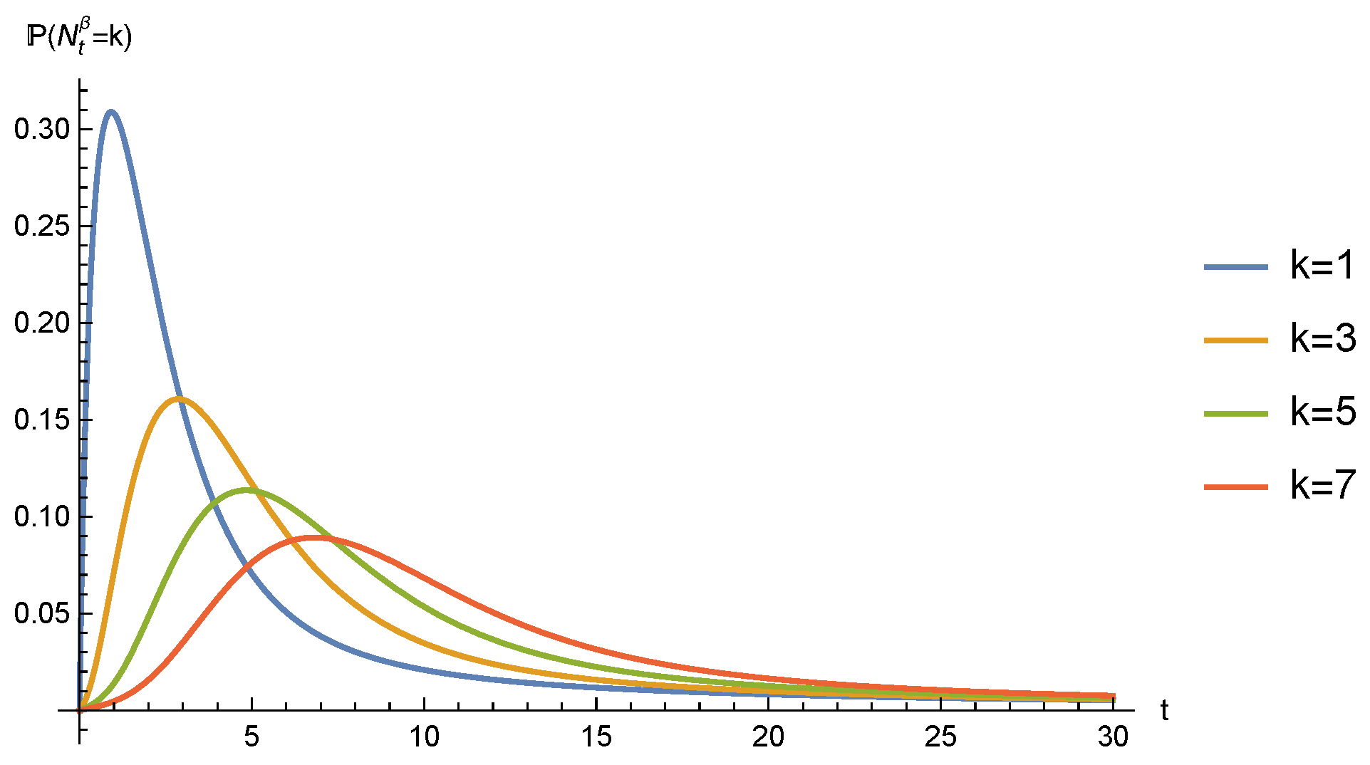
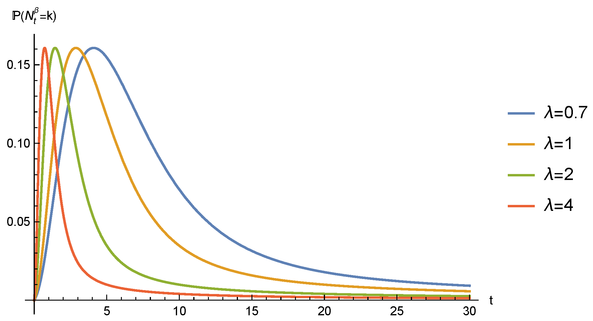
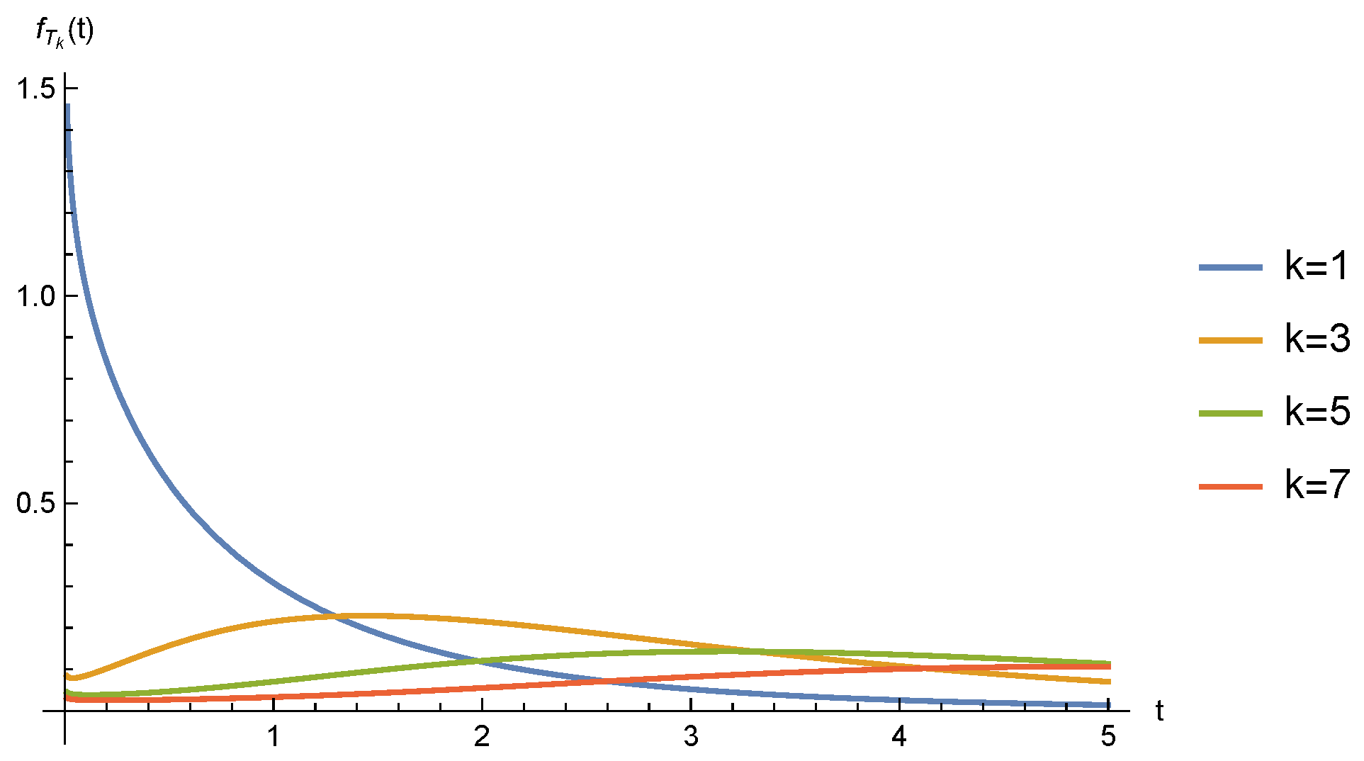
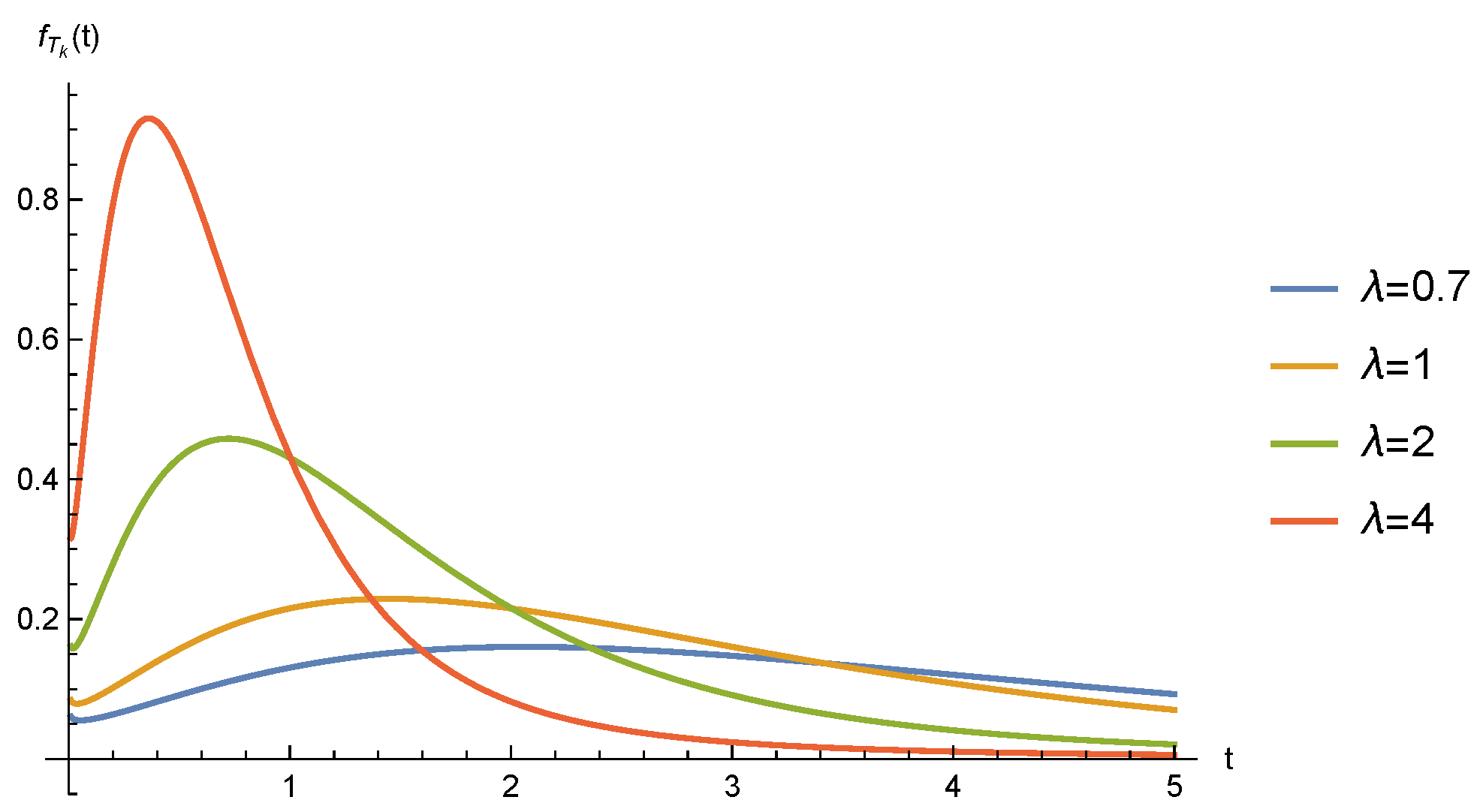
We present a few numerical examples of P N t β = k and f T k ( t ) from Figure 1, Figure 2, Figure 3, Figure 4, Figure 5 and Figure 6.
The Laplace transform of T k is
E e q T k = q L q P T k t = ( 1 ) k Γ ( k ) n = 1 Γ ( β n ) Γ ( β n + 1 k ) λ β q β n ,
which allows us to determine whether { N t β } t 0 is still a renewal process. For k   =   1 ,
E e q T 1 = λ β q β + λ β = E e q τ 1 ,
i.e., τ 1 is Mittag–Leffler distributed with survival function
P ( τ 1 > t ) = E β , 1 λ β t β .
For k   =   2 ,
E e q T 2 = λ β q β ( 1 β ) + λ β q β + λ β 2 = λ β q β + λ β 2 + ( 1 β ) λ β q β q β + λ β 2 .
If τ 1 and τ 2 are independent, then
E e q τ 2 = E e q T 2 E e q T 1 = λ β q β + λ β 2 + ( 1 β ) λ β q β q β + λ β 2 λ β q β + λ β = β λ β q β + λ β + ( 1 β ) ,
which implies that τ 2 is a mixture of Mittag–Leffler distributed random variable with probability β and a mass point at zero with probability 1     β . So, if τ 1 and τ 2 are independent, then they are not equal in distribution and the mass point at zero implies the multiple jumps at one time. Particularly, when β   =   1 , Equation (9) turns out to be
E e q T k = ( 1 ) k Γ ( k ) n = k Γ ( n ) Γ ( n + 1 k ) λ q n = λ q + λ k ,
which is the Laplace transform of a gamma distribution and goes back to a homogeneous Poisson process.
If we denote a β -stable subordinator as { D t β } t 0 , i.e.,
E e q D t β = e t q β ,
then based on the definition,
E t β = inf u 0 : D u β > t , t 0 .
{ E t β } t 0 is non-decreasing and its sample paths are almost surely continuous if { D t β } t 0 is strictly increasing. From Equation (3), it can be seen that { E t β } t 0 possesses non-Markovian with non-stationary and non-independent increments. The probability functions of { D t β } t 0 and { E t β } t 0 are usually in complicated forms, and [20] find the densities of the product, quotient, and power of them in terms of the Fox’s H function. Since
E D t β ρ = t ρ β Γ ( 1 ρ β ) Γ ( 1 ρ ) , ( ρ ) < β ,
then for two independent β -stable processes { D 1 , t β } t 0 and { D 2 , t β } t 0 , we have
E D 1 , t β D 2 , t β ρ = Γ ( 1 ρ β ) Γ ( 1 + ρ β ) Γ ( 1 ρ ) Γ ( 1 + ρ ) , ( ρ ) ( β , β ) .
If we denote L   =   D 1 , t β D 2 , t β β , then L is a Lamperti random variable and its probability density function with respect to the Lebesgue measure on R is
f L ( x ) = sin ( π β ) π β 1 x 2 + 2 x cos ( π β ) + 1 , x > 0 .
See [21,22] for a detailed discussion on the Lamperti law and the stable law. Meanwhile, the Mellin transform of { E t β } t 0 is
E E t β ρ = t β ρ Γ ( 1 + ρ ) Γ ( 1 + β ρ ) .
From [23], for ρ     ( 0 ,   1 ) , the Mellin transform and the Laplace transform of a positive random variable can be connected through
E X ρ = ρ Γ ( 1 ρ ) 0 q ρ 1 1 E e q X d q , ρ ( 0 , 1 ) .
Replacing X with E t β gives
0 q ρ 1 1 E β , 1 q t β d q = t β ρ Γ ( ρ ) Γ ( 1 ρ ) Γ ( 1 + β ρ ) .
The next theorem gives a parallel result to distributional equality Equation 4.
Theorem 2. 
Let { N t β } t 0 be a fractional Poisson process with parameter λ   >   0 and β     ( 0 ,   1 ) . If { U t β } t 0 is a non-negative process such that
f U t β ( x ) = 1 β 1 t H 2 , 2 1 , 1 x t | 1 1 β , 1 β ( 0 , 1 ) 1 1 β , 1 β ( 0 , 1 ) , x > 0 ,
and independent with { N t β } t 0 , then
N t β = d N U t β ,
Proof. 
If Equation (14) is true, then
E e q N t β = E E e q N t β | U t β = E e λ 1 e q U t β = E β , 1 λ β 1 e q β t β ,
which gives
E e q U t β = E β , 1 q β t β .
Applying Equation (12) gives
E U t β ρ = ρ Γ ( 1 ρ ) 0 q ρ 1 1 E β , 1 q β t β d q = ρ Γ ( 1 ρ ) 1 β 0 s ρ β 1 1 E β , 1 s t β d s = ρ Γ ( 1 ρ ) 1 β t β ρ β Γ ρ β Γ 1 ρ β Γ 1 + β ρ β = t ρ Γ 1 ρ β Γ 1 + ρ β Γ ( 1 ρ ) Γ ( 1 + ρ ) , ( ρ ) ( β , β ) .
Finally, applying the inverse Mellin transform gives
f U t β ( x ) = 1 2 π i c i c + i E U t β ρ x 1 ρ d ρ = 1 β 1 2 π i c i c + i t ρ Γ ρ β Γ 1 + ρ β Γ ( ρ ) Γ ( 1 + ρ ) x 1 ρ d ρ = 1 β 1 t 1 2 π i c 1 i c 1 + i Γ 1 β 1 β s Γ 1 1 β + 1 β s Γ ( 1 s ) Γ ( s ) x t s d s = 1 β 1 t H 2 , 2 1 , 1 x t | 1 1 β , 1 β ( 0 , 1 ) 1 1 β , 1 β ( 0 , 1 ) .
Remark 2. 
1.
From Equation (15), { U t β } t 0 does not possess independent and stationary increments.
2.
Comparing Equation (10) and Equation (16), it can be seen that
U t β = d t D 1 , t β D 2 , t β = d t L 1 β = d t E 1 , t β E 2 , t β 1 β ,
which leads to a simpler form of Equation (13) after a change of variable in Equation (11),
f U t β ( x ) = t β π x β 1 sin ( π β ) x 2 β + 2 x β t β cos ( π β ) + t 2 β , x > 0 .
Meanwhile, this expression can be seen from Equation (13) directly,
f U t β ( x ) = 1 β 1 t H 2 , 2 1 , 1 x t | 1 1 β , 1 β ( 0 , 1 ) 1 1 β , 1 β ( 0 , 1 ) = 1 t 1 2 π i c i c + i Γ 1 β y Γ 1 1 β + y Γ ( 1 β y ) Γ ( β y ) x t β y d y = 1 t n = 0 lim y 1 β + n y 1 β n Γ 1 β y Γ 1 1 β + y Γ ( 1 β y ) Γ ( β y ) x t β y = 1 t n = 0 ( 1 ) n Γ ( β n ) Γ ( 1 + β n ) t x ( 1 + β n ) = 1 t n = 0 ( 1 ) n sin ( n π β ) π t x ( 1 + β n ) = 1 π t t x n = 0 sin ( n π β ) x t β n = 1 π 1 x x t β sin ( π β ) x t 2 β + 2 x t β cos ( π β ) + 1 = t β π x β 1 sin ( π β ) x 2 β + 2 x β t β cos ( π β ) + t 2 β .
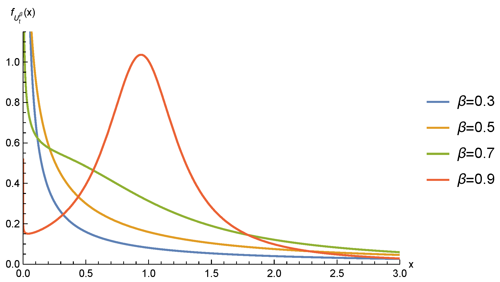
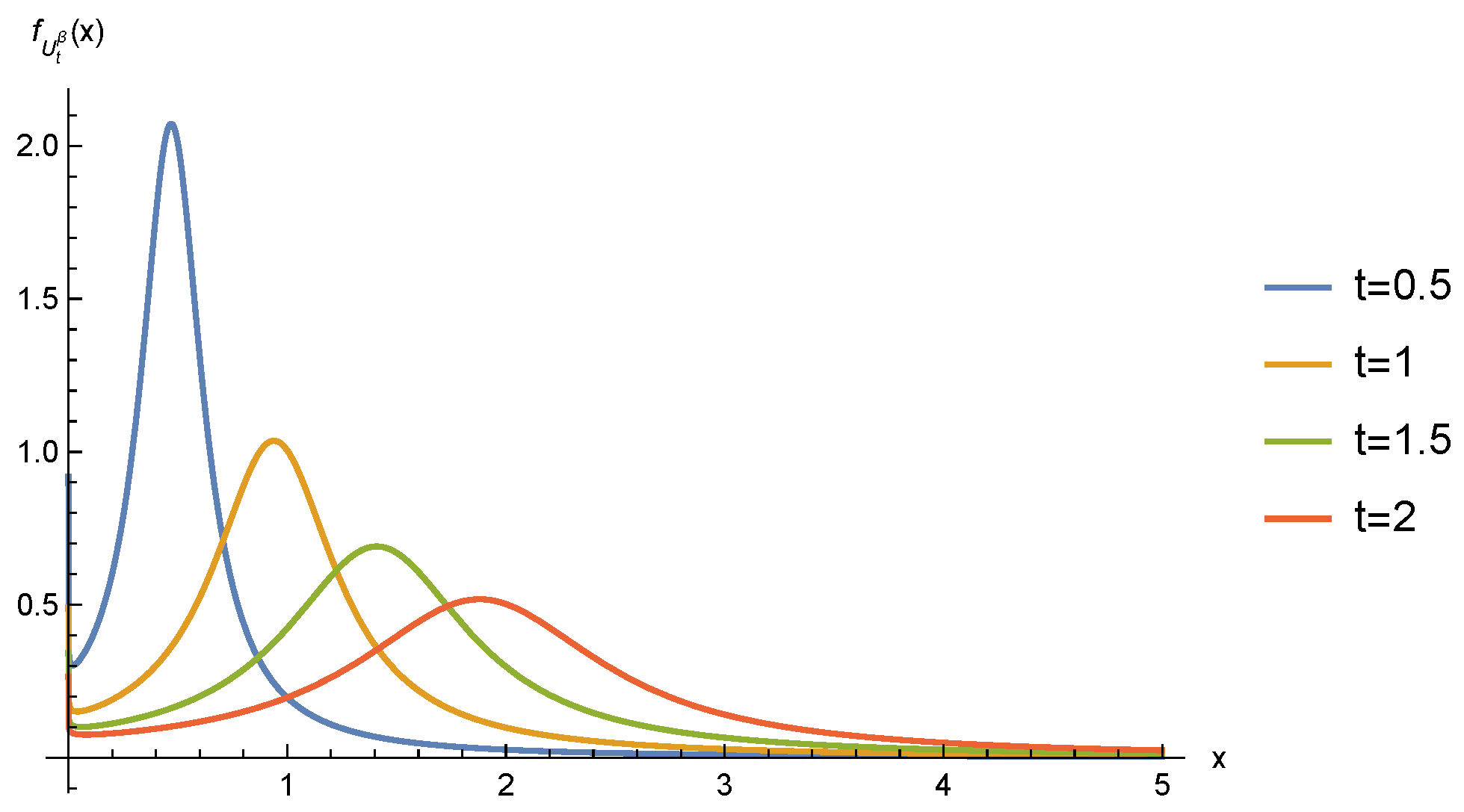
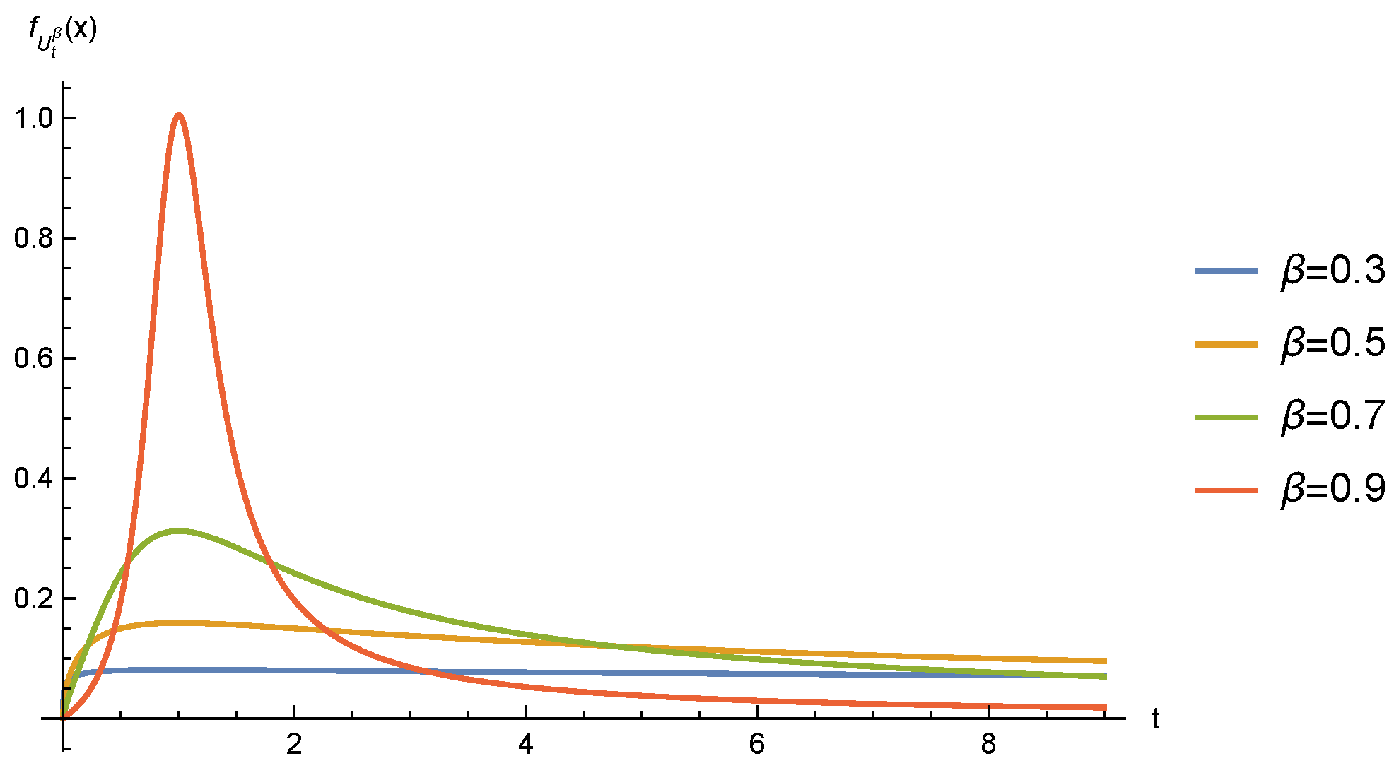
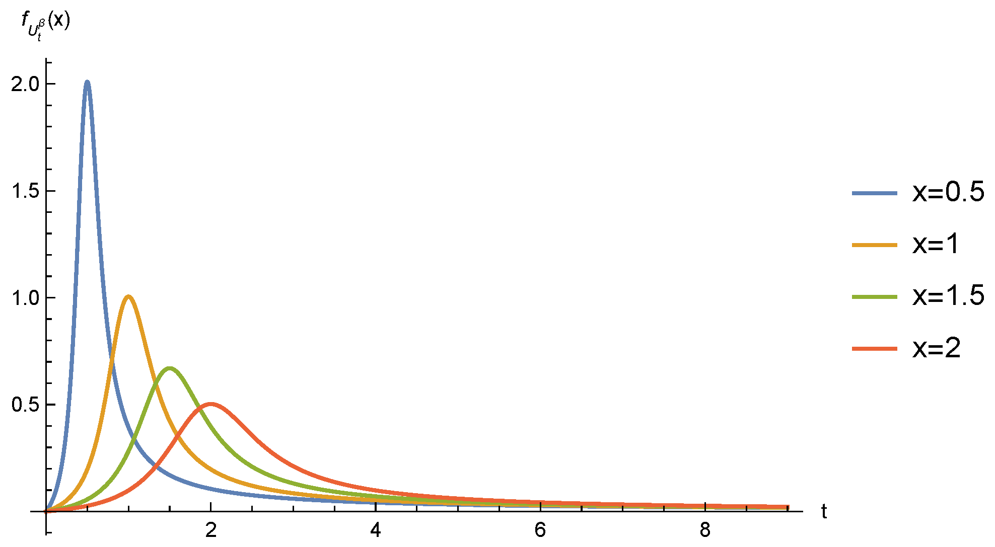
With this simplified expression, we can see that when t     0 , f U t β ( x )     0 and when x     0 , f U t β ( x )     .
3.
From Equation (16), the Mellin transform only exists for ( ρ )     ( β , β ) , and therefore U t β does not have the first moment for t   >   0 . This fits our observation in Theorem 1 that N t β does not have the first moment for t   >   0 either.
We give a few numerical examples of f U t β ( x ) from Figure 7, Figure 8, Figure 9 and Figure 10. In the first two figures, there is a clear sign that the density functions approach to infinity as the variable x tends to zero. In the last two figures, the density functions approach to zero as the variable t tends to zero. These behaviors fit the theoretical analysis on Equation (17).
Equation (13) can be checked through the Laplace transform directly
E e q U t β = 1 β 1 t t H 2 , 3 2 , 1 q t | 0 , 1 β ( 0 , 1 ) ( 0 , 1 ) 0 , 1 β ( 0 , 1 ) = 1 β H 1 , 2 1 , 1 q t | 0 , 1 β 0 , 1 β ( 0 , 1 ) = H 1 , 2 1 , 1 ( q t ) β | ( 0 , 1 ) ( 0 , 1 ) ( 0 , β ) = E β , 1 ( q t ) β .
With the distributional equality Equation (14), Equation (6) can be calculated directly,
P N t β = k = P N U t β = k = 0 ( λ x ) k k ! e λ x P U t β d x = 0 ( λ x ) k k ! e λ x 1 β 1 t 1 2 π i c i c + i Γ 1 β 1 β s Γ 1 1 β + 1 β s Γ ( 1 s ) Γ ( s ) x t s d s d x = 1 k ! 1 β 1 2 π i c 1 i c 1 + i Γ 1 β u Γ 1 1 β u Γ ( k + u ) Γ ( u ) Γ ( 1 u ) ( λ t ) u d u = 1 k ! 1 β 1 2 π i c 1 i c 1 + i Γ 1 β u Γ 1 1 β u Γ ( 1 u ) ( 1 ) k Γ ( u + 1 ) Γ ( u + 1 k ) ( λ t ) u d u = ( 1 ) k k ! 1 β 1 2 π i c 1 i c 1 + i Γ 1 β u Γ 1 1 β u Γ ( 1 k u ) ( λ t ) u d u = ( 1 ) k k ! 1 2 π i c 2 i c 2 + i Γ ( s ) Γ ( 1 s ) Γ ( 1 k β s ) ( λ t ) β s d s = ( 1 ) k k ! E β , 1 k λ β t β .
Corollary 1. 
The Laplace and Mellin transforms of the density function of { U t β } t 0 , where β ( 0 , 1 ) , with respect to the time variable are
0 e s t f U t β ( x ) d t = H 1 , 2 1 , 1 ( s x ) β | 1 1 β , 1 1 1 β , 1 ( 0 , β ) , x > 0 ,
and
0 t ρ f U t β ( x ) d t = x ρ Γ 1 ρ + 1 β Γ 1 + ρ + 1 β Γ ( 2 + ρ ) Γ ( ρ ) , x > 0 .
Proof. 
We first rewrite the density function of U t β as
f U t β ( x ) = 1 β t H 2 , 2 1 , 1 x t | 1 1 β , 1 β ( 0 , 1 ) 1 1 β , 1 β ( 0 , 1 ) = 1 β x H 2 , 2 1 , 1 x t | 1 , 1 β ( 1 , 1 ) 1 , 1 β ( 1 , 1 ) = 1 β x H 2 , 2 1 , 1 t x | 0 , 1 β ( 0 , 1 ) 0 , 1 β ( 0 , 1 ) .
Then, the Laplace transform is
0 e s t f U t β ( x ) d t = 0 e s t 1 β x H 2 , 2 1 , 1 t x | 0 , 1 β ( 0 , 1 ) 0 , 1 β ( 0 , 1 ) d t = 1 β x x H 2 , 3 2 , 1 s x | 1 1 β , 1 β ( 0 , 1 ) ( 0 , 1 ) 1 1 β , 1 β ( 0 , 1 ) = 1 β H 1 , 2 1 , 1 s x | 1 1 β , 1 β 1 1 β , 1 β ( 0 , 1 ) = H 1 , 2 1 , 1 ( s x ) β | 1 1 β , 1 1 1 β , 1 ( 0 , β ) ,
and the Mellin transform is
0 t s 1 f U t β ( x ) d t = 0 t s 1 1 β x H 2 , 2 1 , 1 t x | 0 , 1 β ( 0 , 1 ) 0 , 1 β ( 0 , 1 ) d t = x s β x Γ 1 s β Γ s β Γ ( s ) Γ ( 1 s ) = x s 1 Γ 1 s β Γ 1 + s β Γ ( 1 + s ) Γ ( 1 s ) ,
which completes the proof. □
Let X 1 , X 2 , , X n be a series of n independent and identically distributed random variables with probability density function f X . Denote X ( 1 ) , X ( 2 ) , , X ( n ) as the order statistics of this series if X ( 1 ) X ( k ) X ( n ) , and X ( k ) N t β as the kth order statistic from N t β samples, for k { 1 , , N t β } . The following result is an application of { N t β } t 0 on the order statistics, which shows that the probability of { X ( k ) N t β N t β k } can be expressed as the ratio of probabilities of a fractional Poisson process.
Theorem 3. 
Let { N t β } t 0 be a fractional Poisson process with parameter λ   >   0 , β     ( 0 , 1 ) and { X i } i N be a sequence of i.i.d. random variables with probability distribution function F X ,
P X ( k ) N t β < x N t β k = P N ˜ t β k P N t β k , k N ,
where { N ˜ t β } t 0 is a fractional Poisson process with parameter λ F X   >   0 and β     ( 0 , 1 ) .
Proof. 
By the conditional probability law,
P X ( k ) N t β < x N t β k = n = k P X ( k ) N t β < x , N t β = n P N t β k = n = k P X ( k ) N t β < x N t β = n P N t β = n P N t β k .
The numerator could be computed as
n = k P X ( k ) N t β < x N t β = n P N t β = n = n = k j = k n n j F X j ( x ) 1 F X ( x ) n j ( 1 ) n n ! m = 0 ( λ β t β ) m Γ ( β m + 1 n ) = j = k m = 0 n = j 1 ( n j ) ! j ! F X j ( x ) 1 F X ( x ) n j ( 1 ) n ( λ β t β ) m Γ ( β m + 1 n ) = j = k F X j ( x ) j ! m = 0 ( λ β t β ) m n = 0 1 F X ( x ) n n ! ( 1 ) n + j Γ ( β m + 1 n j ) = j = k F X j ( x ) j ! m = 0 ( λ β t β ) m ( 1 ) j F X β m j ( x ) Γ ( β m + 1 j ) = j = k ( 1 ) j j ! m = 0 λ β F X β ( x ) t β m Γ ( β m + 1 j ) = P ( N ˜ t β k ) .
This completes the proof. □

3. Conclusions and Future Work

In this paper, we discuss a new fractional Poisson process governed by a recursive fractional differential governing equation. The probability distribution function and the Laplace transform of this process are derived. Moreover, this process is equivalent in distribution with a homogeneous Poisson process whose natural time flow is randomized by a Lamperti process. Finally, order statistic from random number samples counted by this fractional Poisson process is studied.
Further research may focus on investigating the distribution properties of the inter-arrival times, generalizing from the first-order differential equation to the nth-order differential equation, and the applications in the risk theory, e.g., the discounted sum counted by this point process.

Funding

This research was supported by The Natural Science Foundation of the Jiangsu Higher Education Institutions of China program [No. 20KJB110019] and the Research Development Fund of Xi’an-Jiaotong Liverpool University [No. RDF-19-02-19].

Acknowledgments

The author thanks the editor and two anonymous reviewers for the valuable comments and suggestions to improve the quality of this paper and clarify the presentation.

Conflicts of Interest

The author declares no conflict of interest.

References

  1. Scalas, E.; Gorenflo, R.; Luckock, H.; Mainardi, F.; Mantelli, M.; Raberto, M. Anomalous waiting times in high-frequency financial data. Quant. Financ. 2004, 4, 695–702. [Google Scholar] [CrossRef] [Green Version]
  2. Kerss, A.; Leonenko, N.N.; Sikorskii, A. Fractional Skellam processes with applications to finance. Fract. Calc. Appl. Anal. Int. J. Theory Appl. 2014, 17, 532. [Google Scholar] [CrossRef]
  3. Jumarie, G. Fractional master equation: Non-standard analysis and Liouville–Riemann derivative. Chaos Solitons Fractals 2001, 12, 2577–2587. [Google Scholar] [CrossRef]
  4. Laskin, N. Fractional Poisson process. Commun. Nonlinear Sci. Numer. Simul. 2003, 8, 201–213. [Google Scholar] [CrossRef]
  5. Repin, O.N.; Saichev, A.I. Fractional Poisson Law. Radiophys. Quantum Electron. 2000, 43, 738–741. [Google Scholar] [CrossRef]
  6. Pillai, R.N. On Mittag-Leffler functions and related distributions. Ann. Inst. Stat. Math. 1990, 42, 157–161. [Google Scholar] [CrossRef]
  7. Mainardi, F.; Gorenflo, R.; Vivoli, A. Beyond the Poisson renewal process: A tutorial survey. J. Comput. Appl. Math. 2007, 205, 725–735. [Google Scholar] [CrossRef] [Green Version]
  8. Beghin, L.; Orsingher, E. Fractional poisson processes and related planar random motions. Electron. J. Probab. 2009, 14, 1790–1826. [Google Scholar] [CrossRef] [Green Version]
  9. Beghin, L.; Orsingher, E. Poisson-type processes governed by fractional and higher-order recursive differential equations. Electron. J. Probab. 2010, 15, 684–709. [Google Scholar] [CrossRef]
  10. Meerschaert, M.; Nane, E.; Vellaisamy, P. The Fractional Poisson Process and the Inverse Stable Subordinator. Electron. J. Probab. 2011, 16, 1600–1620. [Google Scholar] [CrossRef]
  11. Leonenko, N.; Scalas, E.; Trinh, M. The fractional non-homogeneous Poisson process. Stat. Probab. Lett. 2017, 120, 147–156. [Google Scholar] [CrossRef] [Green Version]
  12. Uchaikin, V.V.; Sibatov, R.T. Fractional theory for transport in disordered semiconductors. Commun. Nonlin. Sci. Numer. Simul. 2008, 13, 715–727. [Google Scholar] [CrossRef]
  13. Kumar, A.; Leonenko, N.; Pichler, A. Fractional risk process in insurance. Math. Financ. Econ. 2020, 14, 43. [Google Scholar] [CrossRef] [Green Version]
  14. Wang, X.T.; Wen, Z.X. Poisson fractional processes. Chaos Solitons Fract. 2003, 18, 169–177. [Google Scholar] [CrossRef]
  15. Wang, X.T.; Wen, Z.X.; Zhang, S.Y. Fractional Poisson process (II). Chaos Solitons Fract. 2006, 28, 143–147. [Google Scholar] [CrossRef]
  16. Wang, X.T.; Zhang, S.Y.; Fan, S. Nonhomogeneous fractional Poisson processes. Chaos Solitons Fract. 2007, 31, 236–241. [Google Scholar] [CrossRef]
  17. Lebedev, N.N. Special Functions and Their Applications; Dover Publications: New York, NY, USA, 1972. [Google Scholar]
  18. Mathai, A.M.; Haubold, H.J. Special Functions for Applied Scientists; Springer: New York, NY, USA, 2008. [Google Scholar] [CrossRef] [Green Version]
  19. Mathai, A.; Saxena, R.K.; Haubold, H.J. The H-Function; Springer: New York, NY, USA, 2010. [Google Scholar] [CrossRef]
  20. Kataria, K.; Vellaisamy, P. On densities of the product, quotient and power of independent subordinators. J. Math. Anal. Appl. 2018, 462, 1627–1643. [Google Scholar] [CrossRef] [Green Version]
  21. James, L.F. Lamperti-type laws. Ann. Appl. Probab. 2010, 20, 1303–1340. [Google Scholar] [CrossRef] [Green Version]
  22. Devroye, L.; James, L. On simulation and properties of the stable law. Stat. Methods Appl. 2014, 23, 307–343. [Google Scholar] [CrossRef]
  23. Lin, G.D. On the Mittag-Leffler distributions. J. Stat. Plan. Inference 1998, 74, 1–9. [Google Scholar] [CrossRef]
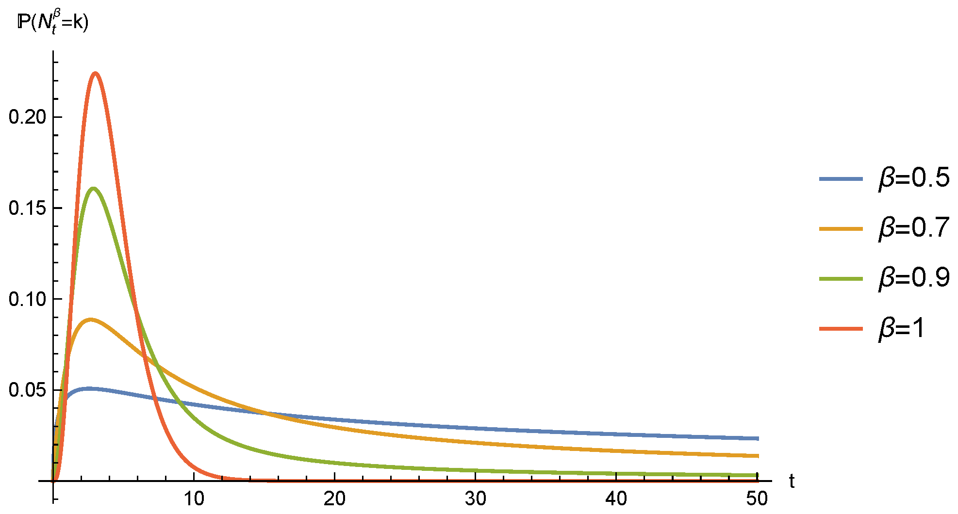
Figure 1. P N t β = 3 with λ = 1 .
Fractalfract 06 00418 g001
Figure 2. P N t 0.9 = k with λ = 1 .
Fractalfract 06 00418 g002
Figure 3. P N t 0.9 = 3 .
Fractalfract 06 00418 g003
Figure 4. f T 3 ( t ) with λ = 1 .
Fractalfract 06 00418 g004
Figure 5. f T k ( t ) with λ = 1 and β = 0.9 .
Fractalfract 06 00418 g005
Figure 6. f T 3 ( t ) with β = 0.9 .
Fractalfract 06 00418 g006
Figure 7. f U 1 β ( x ) .
Fractalfract 06 00418 g007
Figure 8. f U t 0.9 ( x ) .
Fractalfract 06 00418 g008
Figure 9. f U 1 β ( x ) .
Fractalfract 06 00418 g009
Figure 10. f U t 0.9 ( x ) .
Fractalfract 06 00418 g010
Publisher’s Note: MDPI stays neutral with regard to jurisdictional claims in published maps and institutional affiliations.